Assimilation of Earth Observation Data Over Cropland and Grassland Sites into a Simple GPP Model


1
Joint Research Centre (JRC), European Commission, Via E. Fermi 2749, I-21027 Ispra, Italy
2
Max Planck Institute for Biogeochemistry, Hanks Knöll Straße 10, D-07745 Jena, Germany
*
Author to whom correspondence should be addressed.
Remote Sens. 2019, 11(7), 749; https://doi.org/10.3390/rs11070749
Submission received: 11 February 2019
/
Revised: 21 March 2019
/
Accepted: 22 March 2019
/
Published: 27 March 2019
(This article belongs to the Special Issue Remote Sensing of Primary Productivity)
Abstract
:The application of detailed process-oriented simulation models for gross primary production (GPP) estimation is constrained by the scarcity of the data needed for their parametrization. In this manuscript, we present the development and test of the assimilation of Moderate Resolution Imaging Spectroradiometer (MODIS) satellite Normalized Difference Vegetation Index (NDVI) observations into a simple process-based model driven by basic meteorological variables (i.e., global radiation, temperature, precipitation and reference evapotranspiration, all from global circulation models of the European Centre for Medium-Range Weather Forecasts). The model is run at daily time-step using meteorological forcing and provides estimates of GPP and LAI, the latter used to simulate MODIS NDVI though the coupling with the radiative transfer model PROSAIL5B. Modelled GPP is compared with the remote sensing-driven MODIS GPP product (MOD17) and the quality of both estimates are assessed against GPP from European eddy covariance flux sites over crops and grasslands. Model performances in GPP estimation (R2 = 0.67, RMSE = 2.45 gC m−2 d−1, MBE = −0.16 gC m−2 d−1) were shown to outperform those of MOD17 for the investigated sites (R2 = 0.53, RMSE = 3.15 gC m−2 d−1, MBE = −1.08 gC m−2 d−1).
1. Introduction
Gross primary production (GPP) of crops and rangelands is important for understanding CO2 uptake of these ecosystems and ultimately for monitoring the provision of services (food, feed, and fibers) [1]. Detailed crop growth models (CGMs) (e.g., WOFOST, [2]; CROPSYST, [3]), describe plant eco-physiological processes such as light interception and absorption, carbon assimilation, as determined by environmental conditions (weather, soil properties, agro-management, etc.) and vegetation characteristics. Nevertheless, the operational use of such detailed models presents important limitations related to the amount and availability of experimental data needed to properly parameterize, calibrate, and evaluate them, especially over large areas. In fact, complex CGMs require a large number of input parameters whose value is often not available and/or highly uncertain. Moreover, the unrealistic spatial and temporal representation of key parameters representing vegetation characteristics and plant functional traits controlling CO2 uptake was shown to hamper the simulation of GPP at various scales [4,5]. Uncertainties in model inputs are then transferred into large errors in model estimates [6].
Earth observation (EO) data can provide spatially distributed information to increase the reliability and usefulness of crop models [7]. Various methods have been developed to ingest EO data into these models, ranging from the “forcing strategy” (i.e., the direct use of EO as driving variable) to various assimilation techniques. With assimilation, the model does not require EO data as input but the model outputs include some EO variables. For a review of the assimilation techniques see Dorigo et al. [8] and Moulin et al. [9]. Examples of assimilation of EO data into complex ecosystem models for carbon flux estimation are available for forest ecosystems. Quaife et al. [10] assimilated surface reflectance to improve GPP estimation of a pine forest. Bacour et al. [11] assimilated the fraction of photosynthetically active radiation to estimate the net ecosystem exchange at two forest sites. Migliavacca et al. [12] assimilated the normalized difference vegetation index to estimate GPP of a poplar plantation.
The present study aims at estimating crop and grassland GPP with an approach based on the assimilation of EO observations into a simple process-based model of vegetation growth. In view of the spatial application of the model (and the inherent restriction of data availability to calibrate the model), the crop model is kept as simple as possible (i.e., reduced parameterization). In addition, only publicly and freely available EO data and gridded meteorological variables estimated from global circulation model are employed.
The core of the proposed model is composed of a set of equations building on those of the GRAMI model [13,14,15]. Specific differences are detailed in Section 3.1. The growth model is coupled with the canopy radiative transfer (RT) model PROSAIL5B [16] to translate model estimates of leaf area index (LAI) into Normalized Difference Vegetation Index (NDVI) of the Moderate Resolution Imaging Spectroradiometer (MODIS) at the time of actual satellite overpass (i.e., for actual observation and sun geometry), similarly to [12]. Besides this coupling, the canopy RT model was used in the growth model to compute the absorbed photosynthetically active radiation (APAR), thus ensuring internal consistency in the definition of the simplified canopy radiative regime. Finally, the coupled model is “constrained” by a satellite phenology retrieval model [17] that is used to provide a first identification of the likely growth period. For simplicity, we will hereafter refer to such a model scheme as to “Sim model”.
EO data are not used as input (i.e., forcing) but are assimilated into the model to adjust the model parameters and initial conditions. In principle this means that the model benefit from EO data but does not depend on it. Assimilating EO data (i.e., NDVI) into a simple process-based present two main advantages against classical data-driven GPP algorithms: (i) the process of growth is modelled also in absence of EO data (thus increased robustness against missing or noisy EO data); (ii) weather forecasts can be used to run the model to make short-term GPP prediction (given the current model state) that are progressively adjusted when more observations become available. This latter point is of particular interest in view of operational monitoring and forecasting applications.
In this study, GPP estimates by the Sim model are validated using GPP derived at eddy covariance flux sites in Europe and compared to the standard MODIS GPP product (MOD17) used as benchmark [18]. The research questions addressed in this study are: (1) can a simple growth model use modelled meteorological variables and assimilate EO data to adequately simulate crop and grassland GPP? and, (2) what is the estimation accuracy and how does it compare with that of the standard MODIS GPP product?
2. Data
Table 1 provides an overview the data used by the study and their specific use. Detailed description of the datasets is given in Section 2.1, Section 2.2 and Section 2.3.
2.1. Meteorological Data
Meteorological data gathered from the European Centre for Medium-Range Weather Forecasts (ECMWF) forecasting system includes: global radiation, air temperature, precipitation, and potential reference evapotranspiration. Data are from ERA-Interim reanalysis model and are produced at 3-hourly time-step at a spatial resolution of approximately 80 km. Variables are then temporally aggregated to daily mean air temperature and cumulative precipitation and evapotranspiration values. Weather data are taken from the JRC MARSOP project repository [19], where ERA-Interim is down-scaled onto a 25 km reference grid, including bias correction for all elements except precipitation. It is possible that the modelled and downscaled meteorological data may not perfectly represent local meteorology [20] and thus contribute to the mismatch between modelled and measured GPP. However, this topic is not specifically addressed here also because the main aim of the study is to develop and test a methodology for GPP calculation at continental and regional scale and therefore should rely on meteorology from reanalysis, which is therefore here consider as one of the source of uncertainty.
2.2. MODIS NDVI, Reflectances and GPP
As source of EO data we selected MODIS data as it provides a relatively long archive of observations (i.e., from year 2000) and a good compromise between spatial resolution (i.e., 250 m) and temporal resolution of acquisition (i.e., daily revisit). We retrieved NDVI from the MODIS MOD13Q1 and MYD13Q1 version 6 products using the Google Earth Engine. These are 250 m spatial resolution 16-day NDVI composite from Terra and Aqua satellites produced with an 8-day phase shift. Besides NDVI, the following information was retrieved for each observation: reflectances in the blue, red, NIR, and MIR bands, day of acquisition, sun-sensor-target geometry (SZA, Solar Zenith Angle; VZA, View Zenith Angle, RAA, Relative Azimuth Angle), and Vegetation Index (VI) quality and usefulness. Only reliable observations were retained from further processing, i.e., observations with VI reliability greater than two and VI usefulness greater than seven where excluded. MOD09A1 and MYD09A1 (surface reflectance 8-day composite at 500 m) were also acquired to determine the background contribution to canopy NDVI as explained in Section 3.2. In addition, we retrieved the MODIS GPP 8-day version 6 product (MOD17A2H) at 500 m spatial resolution. MODIS GPP 8-day was scaled to mean daily value (gC m−2 d−1) over the 8-day period. We used the flux tower locations to extract the time series of MODIS data by selecting the pixel where the flux tower coordinates falls within.
2.3. Eddy Covariance Flux Tower GPP
Eddy covariance (EC) is an established technique to quantify turbulent exchanges of CO2 between the surface and the atmosphere (for a descrption see Baldocchi et al. [21]; Franz et al. [22]). European flux data have been collected from the European Flux Database Cluster (EFDC, a repository of flux observations for various European projects), and the FLUXNET2015 database (a coordinated effort to harmonize flux observations for as many sites as possible globally [23]). For the purposes of this study, only flux measurements over cropland and grassland were acquired for a total of 58 sites.
Among the different GPP products available in the two datasets we selected half-hourly GPP estimated from net ecosystem exchange (NEE) measurements quality-checked, filtered for low friction velocity conditions, gap-filled and partitioned as consolidated in the FLUXNET methodology [24]. Specifically, we used the GPP product computed using an annual friction velocity threshold to filter NEE, NEE gap-filling based on Marginal Distribution Sampling [25], and finally estimates GPP using night-time flux partitioning [25]. Daily GPP values were computed by aggregating half-hourly GPP estimates, and eventually aggregated to 8-day mean daily value for the validation against modelled GPP. Surface homogeneity of all EC sites was visually inspected using Google Earth to eliminate sites with obvious heterogeneity of land cover within the MODIS pixel (e.g., [26,27]). As a result, only the EC site FR-Avi (Avignon, France) was excluded for further analysis. The location of the retained sites and period covered by flux measurements is shown in Figure 1 (30 cropland sites and 27 grassland sites).
3. Methods
3.1. GPP Model
The vegetation growth model used in this study is composed by a set of equations similar to that of GRAMI model [13,14,15]. The model runs at daily time step and is built around the core equation describing the conversion of absorbed light into gross primary production, GPP [28]:
where i is the day of the year, GPP is the daily gross primary production, εm is the maximum light conversion factor (i.e., the light use efficiency coefficient), εws is the water stress reduction factor to the light use efficiency, PAR is the photosynthetically active radiation and FAPAR is the fraction of the absorbed PAR. The value of εm for crop and grassland targets is set to 1.7 and 1.1 gC m−2 d−1 MJ−1, respectively. These values were derived from a preliminary optimization procedure against EC data of four sites as described in Section 3.4. FAPAR is computed as a function of LAI by the same RT model used to simulate NDVI to ensure internal consistency (see Section 3.2). PAR is estimated as 0.48 * Global Radiation from ECMWF (in MJ m−2) according to Tsubo and Walker [29]. Despite we do not account for direct effect of temperature on εm with an additional stress reduction factor, temperature plays a role in determining εws and leaf senescence (introduced below). In addition, we assume that no photosynthesis occurs when the mean daily temperature is below the base temperature used for the computation of growing degree days (Equation (4)).
A fraction of GPP is used by the plants for respiration, while the remaining net primary production (NPP) is used for the growth. In this simplified modelling we neglect temperature, nitrogen and biomass dependency of maintenance respiration and, based on the findings of Suleau et al. [30], and we consider respiration proportional to GPP. The ratio γ between respiration and GPP was set to 0.25 as in Cui et al. [31].
A fraction of the daily NPP is allocated to leaf tissues according to the following equation:
where ΔLAI is the daily variation of leaf area index (LAI), Pl is the dynamic coefficient of partitioning into leaves, CF is the constant conversion factor from carbon (gC) to dry matter content, SLA is the constant specific leaf area (leaf area per unit weight) and LAIsen is leaf area that is lost through leaf senescence. CF is set to 1/0.45 as in Lobell et al. [32]. SLA (m2 g−1) is subject to optimization (described in Section 3.5) as it is crop- and grassland-type specific and plays a major role in controlling leaf area expansion.
Senescence (LAIsen) and partitioning into leaves (Pl) are modelled using growing degree days (GDD), defined as the sum of the following daily quantity from emergence:
where T is the mean daily air temperature and Tb is the base temperature. Tb is set to the standard value of 0 °C for crops and to −5 °C for grassland according to Fu et al. [33].
∆GDD(i) = Max [T(i) − Tb, 0]
Leaf senescence is empirically modelled as proposed by Maas [14] for the GRAMI model. The LAI emerged at time i with GDD(i) is removed after J(i) growing degree days. The leaf lifespan J(i) of LAI produced on day i is computed as a function of GDD(i) using the following linear equation:
where the parameters c and d control the magnitude of the lifespan as a function of the GDD at emergence. A positive slope (d > 0) increase the lifespan of the leaves emitted later in the season. It is noted that senescence is modulated only as a function of accumulated temperature while other possible stress factors (i.e., water deficiency) are neglected.
J (i) = c + d GDD(i)
In order to select a parametric function to model the temporal evolution of partitioning into leaves we inspected the partitioning look-up tables of the crop growth model WOFOST [34]. Such look-up tables are crop specific, derived from experimental data, and express partitioning into leaves as a function of crop development stage, in turn function of GDD. A preliminary analysis of such data showed that partition into leaves could be well fitted by a three parameters logistic decay function of GDD (data not shown). Although the functional form was selected to mimic partitioning in crops, it appears generic enough to be used for grassland as well.
where Plmax is the curve’s asymptotic maximum value, k is the steepness of the curve, and GDD0 is the x-value of the logistic midpoint.
For the intended application it was convenient to express k and GDD0 as a function of the GDD values GDDmin and GDDmax at which the function takes the actual values of (1 − co) * Plmax and co * Plmax, where co is cutoff value used to numerically deal with the asymptotic function. The cutoff value co is set to 0.05 to yield function values close to its asymptotic maximum (Plmax) and minimum (0). GDDmax is the GDD at which there is (nearly) no more partitioning to leaves. GDDmin is the GDD at which partitioning to leaves is at its maximum, here assumed to be at emergence, where GDD is equal 0. By fixing this latter we reduce the parameters of the logistic curve to two. Using the following intermediary variables:
We can rewrite k and GDD0 of Equation (6) as:
The stress factor εws is computed to account for possible water limitations. The formulation is similar to that of the CASA model [35] where photosynthesis is limited by water availability up to a maximum of 50%:
where AET and PET are the actual and potential evapotranspiration. We assume that all the precipitation can be used for evapotranspiration (i.e., AET equals precipitation). Differently from the CASA model and similar applications (e.g., [36,37]) that compute AET and PET over a period of one to two months (extending backwards in time) we extend back in thermal time, i.e., GDD. In this way, by fixing a GDD period over which precipitation and potential evapotranspiration are considered, we extend back in time over a shorter (longer) period if the temperature was warmer (colder). In addition, considering that more recent weather conditions have a greater effect on the physiological status of the plant we average PET and precipitation with exponentially declining weights when going back into the past (in the GDD dimension). For instance, for the precipitation we compute the following exponentially weighted precipitation (EWP, used in Equation (9) in place of AET):
where x is the thermal time extending back from GDD at time i, CAP is the maximum value of daily precipitation (set to 200 mm, above this threshold water is assumed to exceed storage capacity), and hl is the exponential decay half-life that controls the steepness of the weights decay. It is thus the GDD span in which the weights fall to one half. The hl parameter is set to 180 GDD (that for instance is equivalent to 10 days with mean temperature of 18 °C and 20 days with mean temperature of 9 °C). This formulation depicts an exponentially declining memory of plants to water stress. The exponentially weighted PET (EWPET) is computed in a similar way (but omitting CAP) and used in Equation (9) in place of PET.
εws = min (1, 0.5 + 0.5 AET/PET)
3.2. Radiative Transfer Model
The assimilation of EO data into the model is achieved by linking the canopy reflectance RT model PROSAIL5B [16] to the GPP model described in Section 3.1. While the GPP model simulates the temporal trajectory of the leaf area index (LAI), the link with the canopy RT model allows simulating the NDVI that the MODIS sensor would observe for the satellite overpass time. The RT simulation is performed using the actual sun-target-sensor geometry as specified by the MODIS observations. In order to minimize the number of free parameters, all RT parameters are fixed to nominal values except LAI, SLA, and background reflectance. Although the leaf chlorophyll content can exhibit a seasonal cycle affecting GPP, we opted to keep the model simple and we assumed that actual variation in chlorophyll can be represented in the model by LAI variation alone, having the effect of modulating the total canopy chlorophyll content (LAI x leaf chlorophyll content [38]) when the leaf chlorophyll content is fixed. The values used for the fixed parameters are presented in Table 2. Values refer to literature data for green vegetation (e.g., [39,40]). The fraction of diffuse incoming solar radiation is fixed and was determined by MODTRAN5 [41] simulations for mid-latitude clear sky conditions in summer time.
The reflectance spectrum of the canopy background needed by the RT model to simulate the top of canopy reflectance is determined as follows. For a given pixel, we first select all original NDVI observations with a value smaller than the 5th percentile of the entire NDVI historical distributions (i.e., year 2000—time of simulation). Under the assumption that the time series contains NDVI observations acquired when the green grassland or crop cover is minimal or absent, such observations are considered representative of the background reflectance. As this subset of low-NDVI observations may contain unrealistic outliers (low NDVI values due to undetected cloud cover), we subsample it by selecting the five observations showing the minimum difference between the original NDVI and the NDVI temporally smoothed with the Savitzky-Golay filter [42]. In this way, we discard low-NDVI observations that are far from the smoothed temporal profile (i.e., negative spikes) and may be thus due to undetected clouds rather than absence of vegetation. Background reflectance in the seven MODIS bands coming with MxD09A1 products (see Section 2.2) is computed averaging the reflectances of the selected five observations. Finally, as a full spectrum at 1-nm sampling step is needed by the RT model, the MODIS reflectances are fitted using the Price functions for the soil reflectance [43].
Once the full top of canopy reflectance spectrum (i.e., 400–2500 nm) is simulated with the 1-nm sampling interval used by the RT model, the MODIS relative spectral response functions (http://mcst.gsfc.nasa.gov/calibration/parameters) are used to convolve the spectrum into the MODIS bands. The NDVI is then computed from the MODIS-like red and near infrared bands.
FAPAR used in Equation (1) of the Sim model is computed by PROSAIL5B as the actual instantaneous spectral canopy absorption in the PAR region at 10:00 local solar time. The absorption at this local time is close to the daily integrated value under clear sky condition [44]. The FAPAR value is computed as the weighted average of the spectral canopy absorption in the PAR region (400 to 700 nm). Spectral observations are weighted by their contribution to total incident irradiance at ground level using MODTRAN5 simulations for mid-latitude clear sky conditions in summer time.
3.3. Land Surface Phenology Model
The initial identification of the timing of the onset of growing season is estimated by computing the multi-annual mean of the satellite-based phenological timings retrieved for the pixel temporal profile (2000–2016). Among other phenological timings retrieved fitting a double hyperbolic tangent model to upper envelop of the NDVI time series as described in Meroni et al. [17], we use the number of growing cycles per solar year (either one or two), the start of growing season (SOS) and the time of maximum development (TOM). Besides setting the first guess of the simulation start day, this land surface phenology timings are used to set the first guesses of c of Equation (5) and GDDmax of Equation (8) as the multi-annual average GDD accumulated between SOS and TOM.
3.4. Definition of εmax
Values in the range from 0.86 to 2.5 (gC m−2 d−1 MJ−1) have been reported for grassland and crop εmax in the literature [45,46,47]). Various definitions also exists for it in different communities and in different modelling setups (e.g., depending on weather non-photosynthetic tissues are included in the definition of FAPAR) [48]. Here we used an empirical parametrization that was derived using EC GPP data of two crop and two grass sites randomly extracted from the EC database (BE-Lon and FR-Aur for a total of 17 site-year crop samples; CZ-BK2 and IT-MBo for a total of 17 site-year grassland samples). A nested inversion of the Sim model was run on the two calibration sites. The inversion set-up was configured in standard mode (Section 3.5) and run iteratively for the calibration sites changing the value of εmax in steps of 0.1 between 0.8 and 2.5 gC m−2 d−1 MJ−1. The value minimizing the RMSE between the modelled and observed GPP was then selected. As a result, crop and grass εmax was set to 1.7 and 1.1 gC m−2 d−1 MJ−1, respectively. It is noted that εmax of crops was estimated using sites where C3 crops were numerically more represented (only one year of maize, a C4 crop, is present for the site BE-Lon) and may thus underestimate the εmax of C4 crops (maize in our data sample) (Xin et al., 2015). However, the vast majority of the crop samples is indeed represented by C3 crops.
3.5. Inversion Set-Up
Selected model parameters are derived through model inversion [49]. Here we use model-recalibration as assimilation strategy [8,9] to retrieve the set of model parameters described in Table 3. Recalibration is performed by searching those parameter values that maximize the agreement between the observed MODIS NDVI temporal profile and the simulated one. This is computationally achieved minimizing a cost function defined by the sum of square differences of the two temporal profiles of NDVI. Numerical optimization is performed using Levenberg-Marquardt least-squares constrained minimization (IDL routine MPFIT [50]). Since NDVI may be biased towards low values owing to the presence of undetected clouds, the optimization is adapted to the upper envelope of the observations using an iterative weighting scheme similar to that proposed by Chen et al. [51]. When two growing cycles per solar year are present, they are treated separately.
The iterative minimization requires setting initial values and boundaries for the model parameters (first guess in Table 3).
The water stress factor of Equation (9) is defined on precipitation and evapotranspiration and does not obviously take into account that irrigation water might be administrated to both crops and grasses. As irrigation practices cannot be known a priori, we adopted the following strategy. Optimization is performed twice, without and with water limitation according to Equation (9). The run proving the best fit to observed NDVI is retained. The forward model and the inversion procedure are implemented in IDL (Harris Geospatial Solution).
3.6. Validation
Simulated and observed daily GPP are temporally aggregated to 8-day MODIS temporal resolution. GPP data from 28 crop and 25 grassland EC sites are used in the validation. Simulation performances are assessed analyzing the simulated vs. observed GPP scatter plots in terms of: coefficient of determination (R2), root mean square error (RMSE), and mean bias error (MBE), slope and offset the ordinary-least-squared (OLS) regression model. All these metrics inform about the predictive power of the model as the GPP data were not used for model calibration. Finally, results were compared to those obtained with MODIS GPP product MOD17 that was used as benchmark model. Model performances in space (across sites) and time were further assessed by analyzing (1) the correlation between site averages of annual cumulative GPP observed and modeled, and (2) the ability of the models to track site-level inter-annual variability of GPP. The annual cumulative GPP value is computed summing GPP data over the calendar year (i.e., from 1st of January to 31st December).
4. Results
4.1. Site Examples
The ability of the Sim model to simulate the actual dynamics of GPP is first illustrated on several crops and grassland sites where the model has shown different degrees of realism. Examples of simulated GPP and NDVI compared to the observed time series are reported in Figure 2 and Figure 3 for crop sites and Figure 4, Figure 5 and Figure 6 for grassland sites. For both crops and grassland sites we selected example sites with contrasting performances of the model (i.e., nice vs. poor fit).
Figure 2 and Figure 3 show the observed NDVI and GPP along with the same variables modelled by the Sim model for two EC crop sites. For comparison, the MODIS GPP estimates are also reported.
In the cropland site DE-Kli (Germany, 50.89288°N, 13.52251°E; [57]), rapeseed, winter wheat, maize, and spring barley were cultivated in rotation (Figure 2). The NDVI signal captures the crop growth between sowing and harvest as well as the unmanaged vegetation growth occurring in the fallow land between crop cycles. This is possible thanks to the preliminary application of phenology algorithm that detects two growing seasons per year. The Sim model fits well the observed NDVI and is also able to track GPP temporal evolution with good accuracy (R2 = 0.85, RMSE = 1.66 gC m−2 d−1). Although some under- and over-estimation occurs in some years (e.g., 2009 and 2012, respectively) the Sim model GPP estimates are not affected by systematic underestimation as in the case of the MOD17 product.
In the cropland site IT-BCi (Italy, 40.52375°N, 14.95744°E; [58]) shown in Figure 3 both the Sim model and MOD17 exhibit significant GPP underestimation at high EC GPP levels. Although the Sim model is able to differentiate the two seasons (maize in summer and fennel or rye-grass in winter) depicted by the observed NDVI, it largely underestimates the GPP of the summer crop (i.e., maize). Underestimation of the summer crop occur even though the Sim model does not select water limitation in most of the years (i.e., because the observed NDVI is better matched by model runs without water limitation), which is in agreement with reported irrigation practices. The scatter plots of Figure 3 show that underestimation of the Sim model is nonetheless less severe than the MODIS one. A plausible explanation for this difference may be related to an underestimate of the maximum light use efficiency (εm) that is not able to reproduce the photosynthesis level attained by the C4 crop under a Mediterranean climate and served by irrigation. In fact, both the Sim model and MOD17 use a constant εm of all crops that is likely not representative for this site because the εm of C4 crops is typically larger than that of C3 crops [47]. However, it is noted that in different climatic conditions the model does not underestimate C4 GPP, as for example in the cropland site DE-Kli of Figure 2 where maize was grown in year 2007 and 2012. In general, we do not observe a systematic underestimation of maize GPP (see Section 4.2 and Section 5 for a discussion).
Figure 4, Figure 5 and Figure 6 show the observed NDVI and GPP along with the same variables modelled by the Sim model for three EC grassland sites.
Figure 4 shows the grassland site HU-Bug (Hungary, 47.84690°N, 19.72600°E; [59]), a semi-arid sandy grassland extensively grazed. The Sim model detects two growing cycles per year that are originated from a biomass reduction during the summer due to grazing and/or sever water limitations [60]. In years when no double cycles is visible in the measured GPP, NDVI shows only a moderate reduction during the summer and coherently, the two season modelled by Sim are nearly merged together (e.g., years 2005 and 2006). GPP estimation accuracy is high for both the Sim model and MOD17 for this site (see scatter plots of Figure 4)
Figure 5 shows an example of a grassland site where the GPP estimated by Sim outperforms that of MOD17. It refers to the grassland site of AT-Neu (Austria, 47.11667°N, 11.31750°E; [61]). The Sim model correctly diagnoses one growing cycle per year. Growing cycles are neatly separated by snow cover extending from mid-November to mid-March where measured GPP is close to zero and observed NDVI is very low or missing. While NDVI is nicely fitted by the model, GPP tends to be underestimated by both MOD17 and (to a much lesser extent) by the Sim model. The effect of the fit operated on the upper envelope of the observed NDVI is clearly visible in several years (e.g., 2006, 2007).
Figure 6 shows the results for a grassland site where estimation errors are among the largest in the dataset (IT-Amp, Italy, 41.90410°N, 13.60516°E; [62]). The site is characterized by a distinct summer drought with senescence occurring in June, followed by a cut and subsequent animal grazing and moderate vegetation regrowth. Although the Sim model is able to reproduce this temporal pattern in both NDVI and GPP, it fails to match the GPP magnitude in the main growing period of some years (i.e., 2004, 2006, 2008). It is noted that, in contrast to MOD17 that does not reproduce the GPP reduction between the two growing cycles, the model simulations do detect the break between the cycles and correctly represent the difference in GPP magnitude of the main (spring) and secondary cycle (late summer to autumn).
4.2. Overall Agreement between Modelled and Observed GPP
Density scatter plots of EC measured GPP vs. the GPP estimated by the Sim model and MOD17 are shown Figure 7 and Figure 8 while main statistics are compared Table 4.
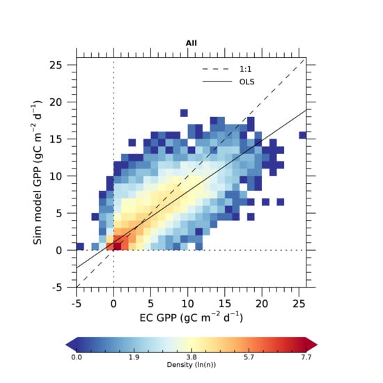
GPP estimated by the Sim model (Figure 7) tracks well the EC GPP with a RMSE of 2.45 gC m−2 d−1 and a small bias (MBE) of −0.16 when all sites are considered together. When considering the two ecosystem types separately, we observed that the RMSE error is slightly larger for crops (2.7 gC m−2 d−1) than for grasslands (2.20 gC m−2 d−1). The MBE is small, positive for crops (0.26 gC m−2 d−1) and negative grasslands (−0.53 gC m−2 d−1). The regression line is in all cases below the 1:1 line indicating a reduction of the variability of estimated GPP as compared to the measured one. Such an effect is larger for MOD17 estimates (Figure 8). Overall, Sim model estimates appears to overestimate EC GPP al low GPP levels and underestimate it at high GPP levels. It is noted that EC GPP can be negative, representing an obvious artifact of the partitioning algorithm (i.e., processing to determine total respiration). Nevertheless, we opted for keeping the EC measurements untouched.
The agreement with EC measurements of GPP is larger for the Sim model with respect to MOD17. Sample scatter and deviation from the 1:1 line is in all cases smaller for the Sim model. Agreement statistics of the Sim Model and MOD 17 are reported in Table 4.
Figure 9 shows the model reliability to predict the total annual GPP and confirms that the Sim model outperforms MOD17.
Maize sites-years are highlighted in green to evaluate whether a negative bias exists for C4 crops (maize in our sample) as consequence of using a fixed value of εm for all crops.
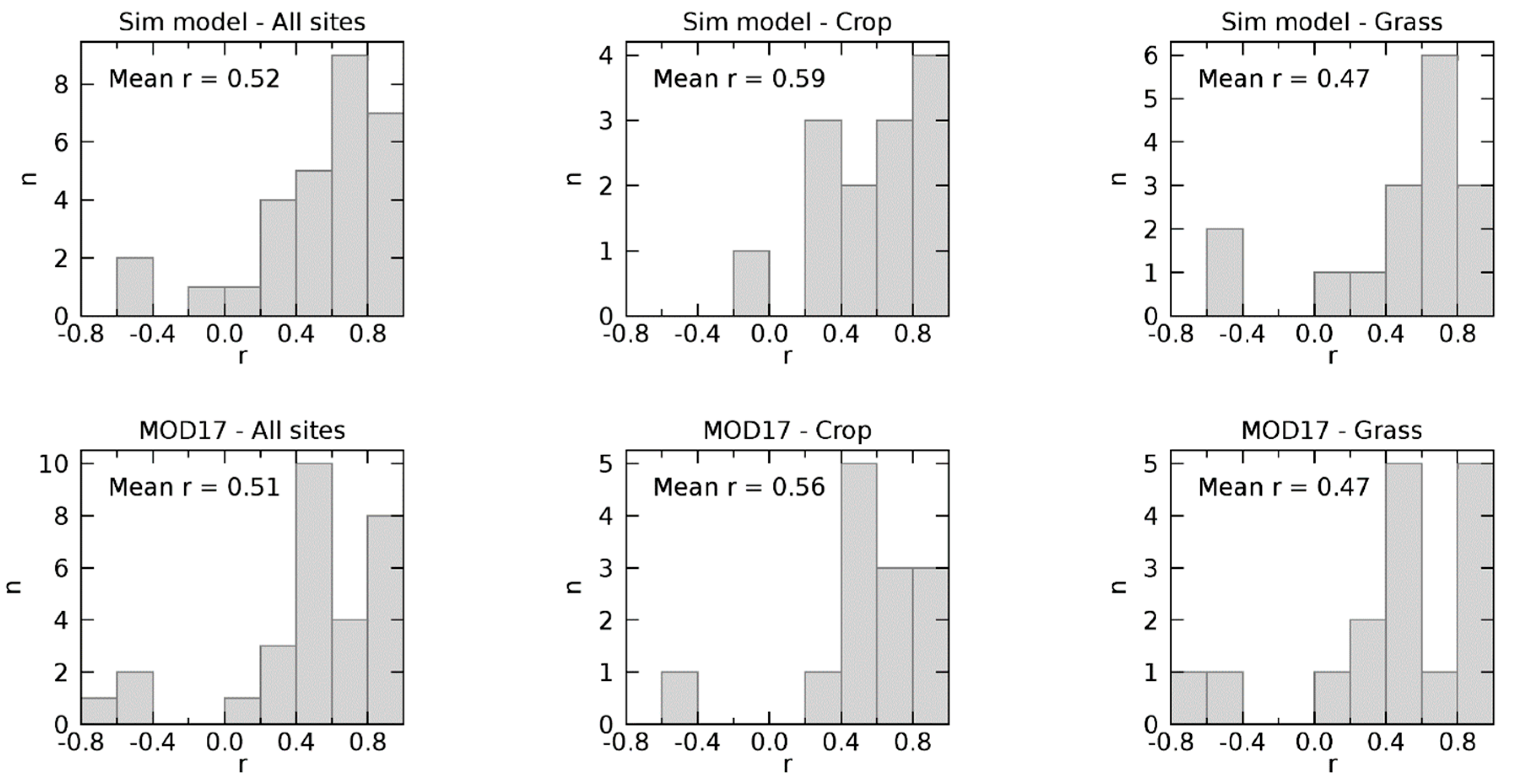
In order to further disentangle the ability of the model in the spatial and temporal dimensions, we compared the mean annual GPP per site (spatial dimension Figure 10) and the site-level statistics of correlation between annual GPP time series (temporal dimension, Figure 11).
The Sim model explains 39% of the spatial variability of GPP with a RMSE 0.34 kgC m−2 y−1 (Figure 10). MOD17 performances are lower (explain variability = 23%, RMSE = 0.52 kgC m−2 y−1) and show consistent underestimate at mid to high annual GPP values. Inter-annual GPP variability is equally and relatively well tracked by both the Sim model and MOD17 (Figure 11). Despite this, examples of sites showing negative correlation are present both when comparing Sim model and MOD17 with EC over time. One example of such sites is the grassland site of IT-Amp reported in Figure 6 where, despite both the Sim model and MOD17 are able to track the intra-annual variation of the GPP, they both fail in modulating the inter-annual variation (r = −0.47 and −0.46 for Sim model and MOD17 respectively).
5. Discussion
Crop and grassland GPP was estimated inverting the Sim model against MODIS 250 m NDVI and validated with EC data. The Sim model showed better performances in GPP estimation as compared to MOD17 that was found to be affected by GPP underestimation, in agreement with Zhu et al. [63]. Table 4 shows that the improvement of the agreement statistics is large when comparing the Sim model with MOD17, e.g., the variance of measured GPP explained by the estimates (i.e., R2) is increased of a 26.4% and RMSE is reduced by a 22.2% when considering all EC sites.
In addition to the obvious differences between the Sim model and MOD17 modelling approaches, we note that the different spatial resolution of the two GPP estimates may contribute to explain the poorer performances of MOD17. In fact, while the Sim model uses NDVI at 250 m, MOD17 is driven by FAPAR at 500 m. Therefore, MOD17 may be more affected by site heterogeneity and less representative of the flux tower footprint [26,27].
It is noted that the removal of the intra-annual variability of GPP operated by the computation of the annual GPP reduces the R2 of both modelling approaches (compare Figure 8 and Figure 9). The Sim model captures better the seasonal dynamics of GPP than the variability among sites (Figure 10) and years (Figure 11) in agreement with the findings of Verma et al. [64] that, comparing a suite of remote sensing based GPP model, found reduced skills in tracking inter-annual as compared to intra-annual GPP variability
Regarding the potential underestimation of C4 crops, we showed that although some maize sites are underestimated by the Sim model, a systematic negative bias of the Sim model is not verified, as maize samples are well distributed above and below the 1:1 line of Figure 9. Moreover, the discrepancies between the Sim model and observed annual GPP seems not influenced by latitude (used to color-code the data points in Figure 9 and Figure 10), and thus climatic differences—essentially temperature—among sites are not introducing an additional bias. This is relevant, as temperature was not considered directly as a reduction factor of εm.
Performances of the Sim model GPP estimation are in line with those of other remote sensing based models calibrated with EC flux data. For instance, similar RMSEs are achieved by Verma et al. [64] over croplands and grasslands using leave-one-out cross-calibration (i.e., n − 1 sites are used to calibrate the model used to predict GPP at the left-out nth site). Larger R2 for GPP estimation (0.78) were achieved by Tramontana et al. [65] using MODIS and meteorological data to train machine learning methods on EC observations. In this study, accuracy was evaluated using 10-fold cross-validation. Despite comparable accuracy, it is noted that the validation protocol is much more conservative in this study: we used four sites for the determining and fixing the value of εmax and the remaining 53 sites for validation.
This study demonstrated that the assimilation of NDVI observations into simple growth model is effective for estimating crop and grassland GPP. In contrast to MOD17 and other approaches using of EO data as input, the proposed model is driven solely by weather variables and remote sensing is used to re-calibrate the model parameters. This opens the possibility of using the model to forecast seasonal GPP within the season, running the inversion using observed NDVI and weather estimates available at a given time in the growing period, and using weather forecast for the remaining of the season.
Currently, the estimation of model parameters during the assimilation of NDVI is time-demanding. This is a disadvantage against data-driven GPP models, where parameter values are known a priori. Processing time currently amounts to about 20 s to optimize the model parameters over a single season on a standard desktop computer. Therefore, an operational wall-to-wall application of the model will require to optimize the code in order to run on parallel computing infrastructures.
Further analysis will focus on evaluating the potential improvements of considering different maximum light use efficiency for C3 and C4 crops and a direct impact of temperature on GPP through a stress factor in addition to that of water stress.
6. Conclusions
A simple crop growth model composed by few equations building on the framework of the GRAMI model was coupled with the canopy radiative transfer model PROSAIL5B and reparametrized against MODIS NDVI observations to estimate GPP of crop and grass ecosystems over Europe. The model requires four meteorological variables as input (incident radiation, air temperature, precipitation and reference potential evapotranspiration) and a preliminary identification of the growing period. In this study, we used meteorological variable estimates from a global circulation model (ECMWF ERA-INTERIM) and the results of a satellite-based land surface phenology retrieval for the initial definition of growing period. GPP estimates from eddy covariance flux sites were used to (1) set the maximum light use efficiency value (2 crop and 2 grassland sites), and (2), validate GPP estimates (28 crop and 25 grassland sites). The approach resulted in acceptable accuracy of GPP 8-day estimates (RMSE = 2.45 gC m−2 d−1, R2 = 0.67, n = 11209). Performances were shown to be improved of about 20% compared to those of standard MODIS MOD17 GPP product, used as benchmark.
Author Contributions
M.M. (Michele Meroni) developed and coded the coupled Sim Model and wrote the majority of the manuscript. D.F. provided essential contributions in preliminary mathematical development of the algorithm. R.L.-L. and M.M. (Mirco Migliavacca) contributed to the conceptual development of the GPP model and provided substantial inputs for the set-up of the validation part. All authors contributed to the writing of the manuscript.
Funding
This research received no external funding.
Acknowledgments
This work used eddy covariance data acquired and shared by the FLUXNET community, including these networks: AmeriFlux, AfriFlux, AsiaFlux, CarboAfrica, CarboEuropeIP, CarboItaly, CarboMont, ChinaFlux, Fluxnet-Canada, GreenGrass, ICOS, KoFlux, LBA, NECC, OzFlux-TERN, TCOS-Siberia, and USCCC. The ERA-Interim reanalysis data are provided by ECMWF and processed by LSCE. The FLUXNET eddy covariance data processing and harmonization was carried out by the European Fluxes Database Cluster, AmeriFlux Management Project, and Fluxdata project of FLUXNET, with the support of CDIAC and ICOS Ecosystem Thematic Center, and the OzFlux, ChinaFlux, and AsiaFlux offices. We thank the following projects for supporting EC measurements and their harmonization: European Fluxes Database Cluster, NitroEurope IP and ECLAIRE. The authors would like to thank all the PIs of eddy covariance sites, including those that shared restricted access data with us. We thank the following PIs for sharing their data and their comments on the present paper: Mark Sutton and Eiko Nemitz (NERC, Edinburgh), Sergiy Medinets (Mechnikov University, Odessa), and Aurore Brut (CESBIO, Toulouse). We thank Josh Hooker, Gregory Duveiller, and Alessandro Cescatti (European Commission, Joint Research Centre) for collecting and harmonizing EC data and for their valuable suggestions. Finally, this research was supported by the Exploratory Research initiative of the European Commission—Joint Research Centre.
Conflicts of Interest
The authors declare no conflict of interest.
References
- Beer, C.; Reichstein, M.; Tomelleri, E.; Ciais, P.; Jung, M.; Carvalhais, N.; Rödenbeck, C.; Arain, M.A.; Baldocchi, D.; Bonan, G.B.; et al. Terrestrial Gross Carbon Dioxide Uptake: Global Distribution and Covariation with Climate. Science 2010, 329, 834–839. [Google Scholar] [CrossRef]
- Supit, L.; Hooijer, A.A.; Van Diepen, C.A. System Description of the WOFOST 6.0 Crop Simulation Model Implemented in CGMS; European Commission Publication Office: Luxembourg, 1994; Volume 1. [Google Scholar]
- Stockle, C.O.; Donatelli, M.; Nelson, R. CropSyst, a cropping systems simulation model. Eur. J. Agron. 2003, 18, 289–307. [Google Scholar] [CrossRef]
- Rogers, A.; Medlyn, B.E.; Dukes, J.S.; Bonan, G.; Caemmerer, S.; Dietze, M.C.; Kattge, J.; Leakey, A.D.; Mercado, L.M.; Niinemets, Ü.; et al. A roadmap for improving the representation of photosynthesis in Earth system models. New Phytol. 2017, 213, 22–42. [Google Scholar] [CrossRef] [PubMed]
- Schaefer, K.; Schwalm, C.R.; Williams, C.; Arain, M.A.; Barr, A.; Chen, J.M.; Davis, K.J.; Dimitrov, D.; Hilton, T.W.; Hollinger, D.Y.; et al. A model-data comparison of gross primary productivity: Results from the North American Carbon Program site synthesis. JGR Biogeosci. 2012, 117, 1–15. [Google Scholar] [CrossRef]
- Hansen, J.W.; Jones, J.W. Scaling-up crop models for climate variability applications. Agric. Syst. 2000, 65, 43–72. [Google Scholar] [CrossRef]
- Machwitz, M.; Giustarini, L.; Bossung, C.; Frantz, D.; Schlerf, M.; Lilienthal, H.; Wandera, L.; Matgen, P.; Hoffmann, L.; Udelhoven, T. Enhanced biomass prediction by assimilating satellite data into a crop growth model. Environ. Model. Softw. 2014, 62, 437–453. [Google Scholar] [CrossRef]
- Dorigo, W.A.; Zurita-Milla, R.; de Wit, A.J.W.; Brazile, J.; Singh, R.; Schaepman, M.E. A review on reflective remote sensing and data assimilation techniques for enhanced agroecosystem modeling. Int. J. Appl. Earth Obs. Geoinf. 2007, 9, 165–193. [Google Scholar] [CrossRef]
- Moulin, S.; Bondeau, A.; Delecolle, R. Combining agricultural crop models and satellite observations: From field to regional scales. Int. J. Remote Sens. 1998, 19, 1021–1036. [Google Scholar] [CrossRef]
- Quaife, T.; Lewis, P.; De Kauwe, M.; Williams, M.; Law, B.E.; Disney, M.; Bowyer, P. Assimilating canopy reflectance data into an ecosystem model with an Ensemble Kalman Filter. Remote Sens. Environ. 2008, 112, 1347–1364. [Google Scholar] [CrossRef]
- Bacour, C.; Peylin, P.; Macbean, N.; Rayner, P.J.; Delage, F.; Chevallier, F.; Weiss, M.; Demarty, J.; Santaren, D.; Baret, F.; et al. Joint assimilation of eddy covariance flux measurements and FAPAR products over temperate forests within a process-oriented biosphere model. J. Geophys. Res. Biogeosci. 2015, 120, 1839–1857. [Google Scholar] [CrossRef]
- Migliavacca, M.; Meroni, M.; Busetto, L.; Colombo, R.; Zenone, T.; Matteucci, G.; Manca, G.; Seufert, G. Modeling Gross Primary Production of Agro-Forestry Ecosystems by Assimilation of Satellite-Derived Information in a Process-Based Model. Sensors 2009, 9, 922–942. [Google Scholar] [CrossRef]
- Ko, J.; Maas, S.J.; Mauget, S.; Piccinni, G.; Wanjura, D. Modeling Water-Stressed Cotton Growth Using Within-Season Remote Sensing Data. Agron. J. 2006, 98, 1600. [Google Scholar] [CrossRef]
- Maas, S.J. Parameterized Model of Gramineous Crop Growth: I. Leaf Area and Dry Mass Simulation. Agron. J. 1993, 85, 348–353. [Google Scholar] [CrossRef]
- Maas, S.J. Parameterized Model of Gramineous Crop Growth: II. Within-Season Simulation Calibration. Agron. J. 1993, 85, 354–358. [Google Scholar] [CrossRef]
- Jacquemoud, S.; Verhoef, W.; Baret, F.; Bacour, C.; Zarco-Tejada, P.J.; Asner, G.P.; François, C.; Ustin, S.L. PROSPECT + SAIL models: A review of use for vegetation characterization. Remote Sens. Environ. 2009, 113, S56–S66. [Google Scholar] [CrossRef]
- Meroni, M.; Verstraete, M.M.; Rembold, F.; Urbano, F.; Kayitakire, F. A phenology-based method to derive biomass production anomalies for food security monitoring in the Horn of Africa. Int. J. Remote Sens. 2014, 35, 2472–2492. [Google Scholar] [CrossRef]
- Heinsch, F.A.; Zhao, M.; Running, S.W.; Kimball, J.S.; Nemani, R.R.; Davis, K.J.; Bolstad, P.V.; Cook, B.D.; Desai, A.R.; Ricciuto, D.M.; et al. Evaluation of Remote Sensing Based Terrestrial Productivity From MODIS Using Regional Tower Eddy Flux Network Observations. IEEE Trans. Geosci. Remote Sens. 2006, 44, 1908–1925. [Google Scholar] [CrossRef]
- MARS Crop Yield Forecasting System. WikiMCYFS [WWW Document]. 2018. Available online: https://marswiki.jrc.ec.europa.eu/agri4castwiki/index.php/Welcome_to_WikiMCYFS (accessed on 15 January 2019).
- Vuichard, N.; Papale, D. Filling the gaps in meteorological continuous data measured at FLUXNET sites with ERA-Interim reanalysis. Earth Syst. Sci. Data 2015, 7, 157–171. [Google Scholar] [CrossRef]
- Baldocchi, D.; Falge, E.; Gu, L.; Olson, R.; Hollinger, D.; Running, S.; Anthoni, P.; Bernhofer, C.; Davis, K.; Evans, R.; et al. FLUXNET: A New Tool to Study the Temporal and Spatial Variability of Ecosystem-Scale Carbon Dioxide, Water Vapor, and Energy Flux Densities. Bull. Am. Meteorol. Soc. 2001, 2415–2434. [Google Scholar] [CrossRef]
- Franz, D.; Acosta, M.; Globe, C.; Altimir, N.; Arriga, N. Towards long-term standardised carbon and greenhouse gas observations for monitoring Europe’ s terrestrial ecosystems: A review. Int. Agrophys. 2018, 32, 439–455. [Google Scholar] [CrossRef]
- Pastorello, G.Z.; Papale, D.; Chu, H.; Trotta, C.; Agarwal, D.A.; Canfora, E.; Baldocchi, D.D.; Torn, M.S. A New Data Set to Keep a Sharper Eye on Land-Air Exchanges; Eos: Washington, DC, USA, 2017; Volume 98. [Google Scholar] [CrossRef]
- Papale, D.; Reichstein, M.; Aubinet, M.; Canfora, E.; Bernhofer, C.; Kutsch, W.; Longdoz, B.; Rambal, S.; Valentini, R.; Vesala, T.; et al. Towards a standardized processing of Net Ecosystem Exchange measured with eddy covariance technique: Algorithms and uncertainty estimation. Biogeosciences 2006, 3, 571–583. [Google Scholar] [CrossRef]
- Reichstein, M.; Falge, E.; Baldocchi, D.; Papale, D.; Aubinet, M.; Berbigier, P.; Bernhofer, C.; Buchmann, N.; Gilmanov, T.; Granier, A.; et al. On the separation of net ecosystem exchange into assimilation and ecosystem respiration: Review and improved algorithm. Glob. Chang. Biol. 2005, 11, 1424–1439. [Google Scholar] [CrossRef]
- Cescatti, A.; Marcolla, B.; Santhana, S.K.; Yun, J.; Román, M.O.; Yang, X.; Ciais, P.; Cook, R.B.; Law, B.E.; Matteucci, G.; et al. Intercomparison of MODIS albedo retrievals and in situ measurements across the global FLUXNET network. Remote Sens. Environ. 2012, 121, 323–334. [Google Scholar] [CrossRef]
- Migliavacca, M.; Reichstein, M.; Richardson, A.D.; Mahecha, M.; Cremonese, E.; Delpierre, N.; Galvagno, M.; Law, B.E.; Wohlfahrt, G.; Black, A.; et al. Influence of physiological phenology on the seasonal pattern of ecosystem respiration in deciduous forests. Glob. Chang. Biol. 2015, 21, 363–376. [Google Scholar] [CrossRef] [PubMed]
- Monteith, J.L. Solar radiation and productivity in tropical ecosystems. J. Appl. Ecol. 1972, 9, 747–766. [Google Scholar] [CrossRef]
- Tsubo, M.; Walker, S. Relationships between photosynthetically active radiation and clearness index at Bloemfontein, South Africa. Theor. Appl. Climatol. 2005, 80, 17–25. [Google Scholar] [CrossRef]
- Suleau, M.; Moureaux, C.; Dufranne, D.; Buysse, P.; Bodson, B.; Destain, J.P.; Heinesch, B.; Debacq, A.; Aubinet, M. Respiration of three Belgian crops: Partitioning of total ecosystem respiration in its heterotrophic, above- and below-ground autotrophic components. Agric. For. Meteorol. 2011, 151, 633–643. [Google Scholar] [CrossRef]
- Cui, T.; Wang, Y.; Sun, R.; Qiao, C.; Fan, W.; Jiang, G.; Hao, L.; Zhang, L. Estimating vegetation primary production in the heihe river basin of China with multi-source and multi-scale data. PLoS ONE 2016, 11, e0153971. [Google Scholar] [CrossRef] [PubMed]
- Lobell, D.B.; Asner, G.P.; Field, C.B.; Tucker, C.J.; Los, S.O. Satelite estimates of productivity and klight use efficiency in United States agriculture, 1982–98. Glob. Chance Biol. 2002, 8, 722–735. [Google Scholar] [CrossRef]
- Fu, Y.; Zhang, H.; Dong, W.; Yuan, W. Comparison of Phenology Models for Predicting the Onset of Growing Season over the Northern Hemisphere. PLoS ONE 2014, 9, e0109544. [Google Scholar] [CrossRef] [PubMed]
- Boogaard, H.L.; Van Diepen, C.A.; Rötter, R.P.; Cabrera, J.M.C.; Van Laar, H.H. WOFOST 7.1.7—User’s Guide; University of Wageningen: Wageningen, The Netherlands, 2014. [Google Scholar]
- Field, C.B.; Randerson, J.T.; Malmström, C.M. Global net primary production: Combining ecology and remote sensing. Remote Sens. Environ. 1995, 51, 74–88. [Google Scholar] [CrossRef]
- Maselli, F.; Chiesi, M.; Brilli, L.; Moriondo, M. Simulation of olive fruit yield in Tuscany through the integration of remote sensing and ground data. Ecol. Modell. 2012, 244, 1–12. [Google Scholar] [CrossRef]
- Maselli, F.; Papale, D.; Puletti, N.; Chirici, G.; Corona, P. Combining remote sensing and ancillary data to monitor the gross productivity of water-limited forest ecosystems. Remote Sens. Environ. 2009, 113, 657–667. [Google Scholar] [CrossRef]
- Gitelson, A.A.; Peng, Y.; Arkebauer, T.J.; Schepers, J. Relationships between gross primary production, green LAI, and canopy chlorophyll content in maize: Implications for remote sensing of primary production. Remote Sens. Environ. 2014, 144, 65–72. [Google Scholar] [CrossRef]
- Atzberger, C.; Darvishzadeh, R.; Schlerf, M.; Le Maire, G. Suitability and adaptation of PROSAIL radiative transfer model for hyperspectral grassland studies. Remote Sens. Lett. 2013, 4, 55–64. [Google Scholar] [CrossRef]
- Vohland, M.; Jarmer, T. Estimating structural and biochemical parameters for grassland from spectroradiometer data by radiative transfer modelling (PROSPECT+SAIL). Int. J. Remote Sens. 2008, 29, 191–209. [Google Scholar] [CrossRef]
- Berk, A.; Cooley, T.W.; Anderson, G.P.; Acharya, P.K.; Bernstein, L.S.; Muratov, L.; Lee, J.; Fox, M.J.; Adler-Golden, S.M.; Chetwynd, J.H.; et al. MODTRAN5: A reformulated atmospheric band model with auxiliary species and practical multiple scattering options. Proc. SPIE 2004, 5571. Remote Sensing of Clouds and the Atmosphere IX, (30 November 2004). [Google Scholar] [CrossRef]
- Savitzky, A.; Golay, M.J.E. Smoothing and differentiation of data by simplified least squares procedures. Anal. Chem. 1964, 36, 1627–1639. [Google Scholar] [CrossRef]
- Price, J.C. On the Information-Content of Soil Reflectance Spectra. Remote Sens. Environ. 1990, 33, 113–121. [Google Scholar] [CrossRef]
- Claverie, M.; Vermote, E.F.; Weiss, M.; Baret, F.; Hagolle, O.; Demarez, V. Validation of coarse spatial resolution LAI and FAPAR time series over cropland in southwest France. Remote Sens. Environ. 2013, 139, 216–230. [Google Scholar] [CrossRef]
- Dong, T.; Liu, J.; Qian, B.; Jing, Q.; Croft, H.; Chen, J.; Wang, J.; Huffman, T.; Shang, J.; Chen, P. Deriving Maximum Light Use Efficiency From Crop Growth Model and Satellite Data to Improve Crop Biomass Estimation. In IEEE Journal of Selected Topics in Applied Earth Observations and Remote Sensing; IEEE: Piscataway, NJ, USA, 2017; Volume 10, pp. 104–117. [Google Scholar]
- Running, S.W.; Zhao, M.S. Daily GPP and Annual NPP (MOD17A2/A3) Products User’s Guide; The University of Montana: Missoula, MT, USA, 2015. [Google Scholar]
- Xin, Q.; Broich, M.; Suyker, A.E.; Yu, L.; Gong, P. Multi-scale evaluation of light use efficiency in MODIS gross primary productivity for croplands in the Midwestern United States. Agric. For. Meteorol. 2015, 201, 111–119. [Google Scholar] [CrossRef]
- Gitelson, A.A.; Gamon, J.A. The need for a common basis for defining light-use efficiency: Implications for productivity estimation. Remote Sens. Environ. 2015, 156, 196–201. [Google Scholar] [CrossRef]
- Kimes, D.; Knyazikhin, Y.; Privette, J.L.; Abuelgasim, A.A.; Gao, F. Inversion methods for physically-based models. Remote Sens. Rev. 2000, 18, 381–439. [Google Scholar] [CrossRef]
- Markwardt, C.B. Non-Linear Least Squares Fitting in IDL with MPFIT. In Astronomical Data Analysis Software and Systems XVIII; Bohlender, D., Durand, D., Dowler, P., Eds.; (Astronomical Society of the Pacific: San Francisco): Quebec, QC, Canada, 2009; pp. 251–254. [Google Scholar]
- Chen, J.; Jonsson, P.; Tamura, M.; Gu, Z.; Matsushita, B.; Eklundh, L. A simple method for reconstructing a high-quality NDVI time-series data set based on the Savitzky-Golay filter. Remote Sens. Environ. 2004, 91, 332–344. [Google Scholar] [CrossRef]
- González-Sanpedro, M.C.; Le Toan, T.; Moreno, J.; Kergoat, L.; Rubio, E. Seasonal variations of leaf area index of agricultural fields retrieved from Landsat data. Remote Sens. Environ. 2008, 112, 810–824. [Google Scholar] [CrossRef]
- Grubb, P.J.; Marañón, T.; Pugnaire, F.I.; Sack, L. Relationships between specific leaf area and leaf composition in succulent and non-succulent species of contrasting semi-desert communities in south-eastern Spain. J. Arid Environ. 2015, 118, 69–83. [Google Scholar] [CrossRef]
- Knops, J.; Reinhart, K. Specific Leaf Area Along a Nitrogen Fertilization Gradient. Am. Midl. Nat. 2000, 144, 265–272. [Google Scholar] [CrossRef]
- Wellstein, C.; Poschlod, P.; Gohlke, A.; Chelli, S.; Campetella, G.; Rosbakh, S.; Canullo, R.; Kreyling, J.; Jentsch, A.; Beierkuhnlein, C. Effects of extreme drought on specific leaf area of grassland species: A meta-analysis of experimental studies in temperate and sub-Mediterranean systems. Glob. Chang. Biol. 2017, 23, 2473–2481. [Google Scholar] [CrossRef] [PubMed]
- Boons-Prins, E.R.; de Koning, G.H.J.; Van Diepen, C.A.; Penning de Vries, F.W.T. Crop Specific Simulation Parameters for Yield Forecasting across the European Community; Simulation Reports CABO-TT 32; University of Wageningen: Wageningen, The Netherlands, 1993. [Google Scholar]
- Prescher, A.; Grünwald, T.; Bernhofer, C. Agricultural and Forest Meteorology Land use regulates carbon budgets in eastern Germany: From NEE to NBP. Agric. For. Meteorol. 2010, 150, 1016–1025. [Google Scholar] [CrossRef]
- Kutsch, W.L.; Aubinet, M.; Buchmann, N.; Smith, P.; Osborne, B.; Eugster, W.; Wattenbach, M.; Schrumpf, M.; Schulze, E.D.; Tomelleri, E.; et al. Agriculture, Ecosystems and Environment The net biome production of full crop rotations in Europe. Agric. Ecosyst. Environ. 2010, 139, 336–345. [Google Scholar] [CrossRef]
- Nagy, Z.; Pintér, K.; Pavelka, M.; Darenová, E.; Balogh, J. Carbon fluxes of surfaces vs. ecosystems: Advantages of measuring eddy covariance and soil respiration simultaneously in dry grassland ecosystems. Biogeosciences 2011, 8, 2523–2534. [Google Scholar] [CrossRef]
- Nagy, Z.; Pinter, K.; Czobel, S.; Balogh, J.; Horvath, L.; Foti, S.; Barcza, Z.; Weidinger, T.; Csintalan, Z.; Dinh, N.Q.; et al. The carbon budget of semi-arid grassland in a wet and a dry year in Hungary. Agric. Ecosyst. Environ. 2007, 121, 21–29. [Google Scholar] [CrossRef]
- Wohlfahrt, G.; Anfang, C.; Bahn, M.; Haslwanter, A.; Newesely, C.; Schmitt, M.; Dro, M. Quantifying nighttime ecosystem respiration of a meadow using eddy covariance, chambers and modelling. Agric. For. Meteorol. 2005, 128, 141–162. [Google Scholar] [CrossRef]
- Wohlfahrt, G.; Anderson-dunn, M.; Bahn, M.; Berninger, F.; Campbell, C.; Carrara, A.; Cescatti, A.; Christensen, T.; Dore, S.; Friborg, T.; et al. Biotic, Abiotic, and Management Controls on the Net Ecosystem CO2 Exchange of European Mountain Grassland Ecosystems. Ecosystems 2008, 1338–1351. [Google Scholar] [CrossRef]
- Zhu, X.; Pei, Y.; Zheng, Z.; Dong, J.; Zhang, Y.; Wang, J.; Chen, L.; Doughty, R.B.; Zhang, G.; Xiao, X. Underestimates of Grassland Gross Primary Production in MODIS Standard Products. Remote Sens. 2018, 10, 1771. [Google Scholar] [CrossRef]
- Verma, M.; Friedl, M.A.; Law, B.E.; Bonal, D.; Kiely, G.; Black, T.A.; Wohlfahrt, G.; Moors, E.J.; Montagnani, L.; Marcolla, B.; et al. Improving the performance of remote sensing models for capturing intra- and inter-annual variations in daily GPP: An analysis using global FLUXNET tower data. Agric. For. Meteorol. 2015, 214–215, 416–429. [Google Scholar] [CrossRef]
- Tramontana, G.; Jung, M.; Schwalm, C.R.; Ichii, K.; Camps-valls, G.; Raduly, B.; Reichstein, M.; Altaf Arain, M.; Cescatti, A.; Kiely, G.; et al. Predicting carbon dioxide and energy fluxes across global FLUXNET sites with regression algorithms. Biogeosciences 2016, 13, 4291–4313. [Google Scholar] [CrossRef]
Figure 1.
Location of eddy covariance (EC) sites and period covered by flux measurements. Green cross are for grassland sites whereas orange dots are for cropland sites.
Figure 1.
Location of eddy covariance (EC) sites and period covered by flux measurements. Green cross are for grassland sites whereas orange dots are for cropland sites.
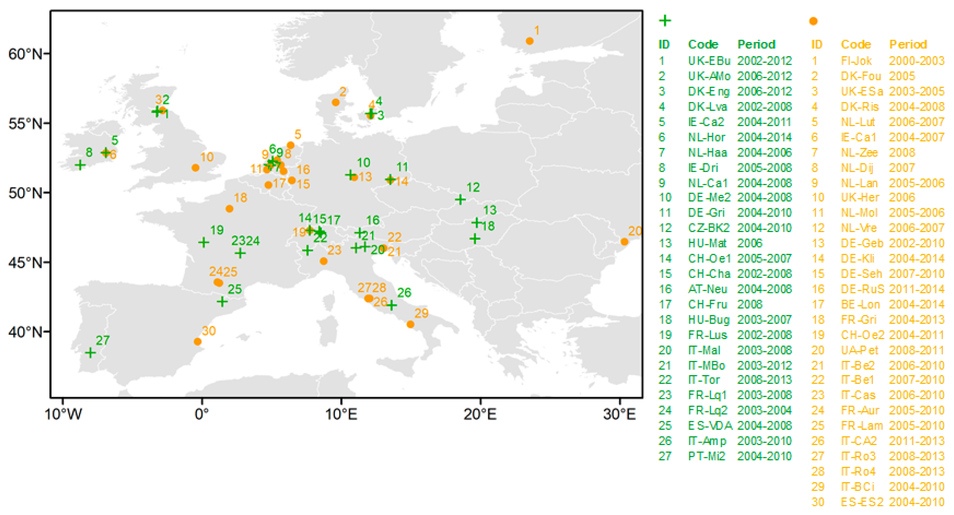
Figure 2.
Observed and modelled GPP and NDVI for the crop site DE-Kli. Left panels: (top) time series of GPP from eddy covariance measurements (EC), Sim model (Sim), and MODIS GPP (MOD17); (bottom) observed (MODIS) and simulated NDVI (Sim). Right panels: scatter plots of EC GPP versus GPP simulated by the Sim model (top panel) and MOD17 GPP (bottom panel). For the right panels: dashed black line is the 1:1 line, blue continues line is the linear regression; root mean square error (RMSE) between modelled and observed GPP and the coefficient of determination (R2) of the linear regression are reported.
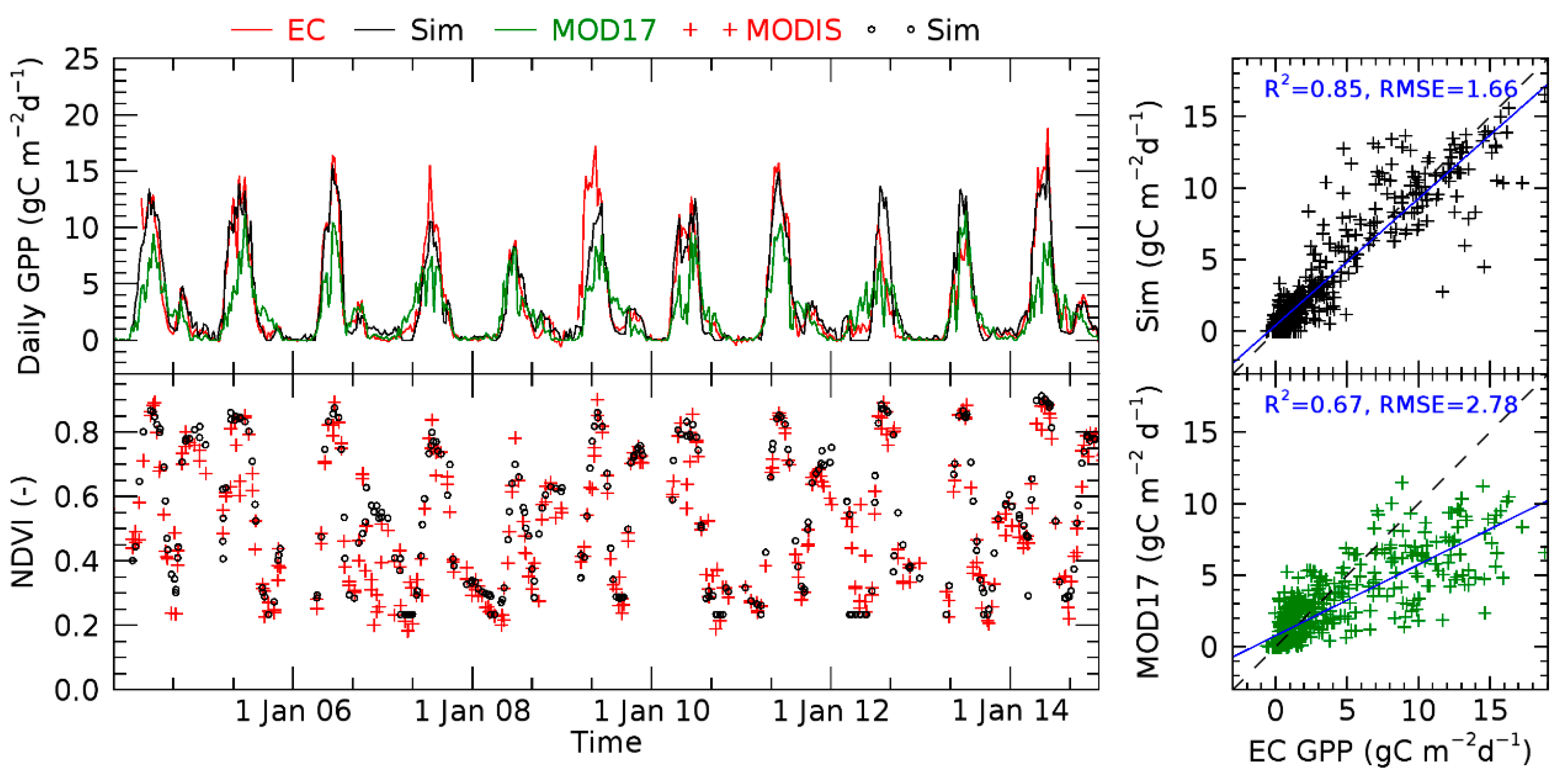
Figure 3.
Observed and modelled GPP and NDVI for the cropland site IT-BCi. Description of plots as Figure 2.
Figure 3.
Observed and modelled GPP and NDVI for the cropland site IT-BCi. Description of plots as Figure 2.
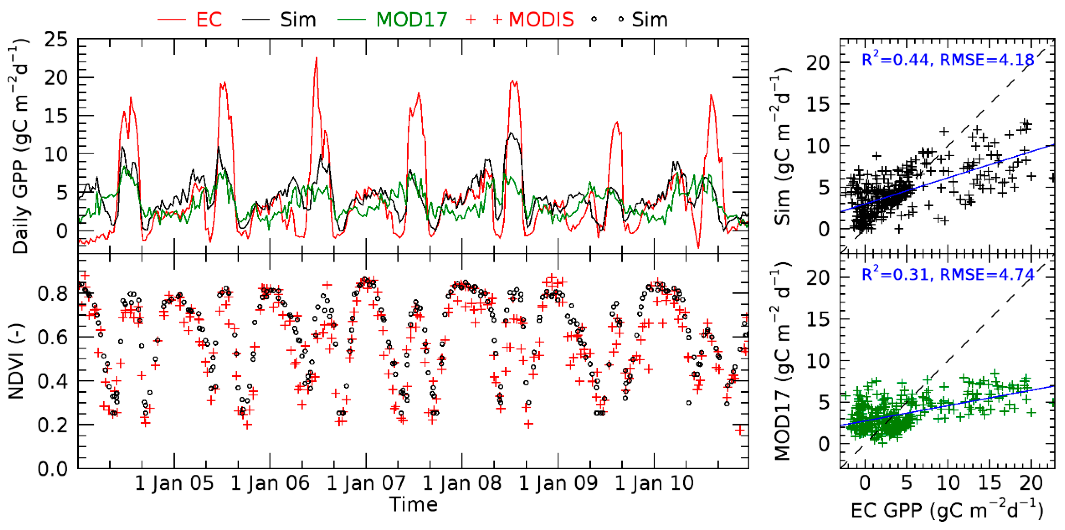
Figure 4.
Observed and modelled GPP and NDVI for the grassland site HU-Bug. Description of plots as Figure 2.
Figure 4.
Observed and modelled GPP and NDVI for the grassland site HU-Bug. Description of plots as Figure 2.
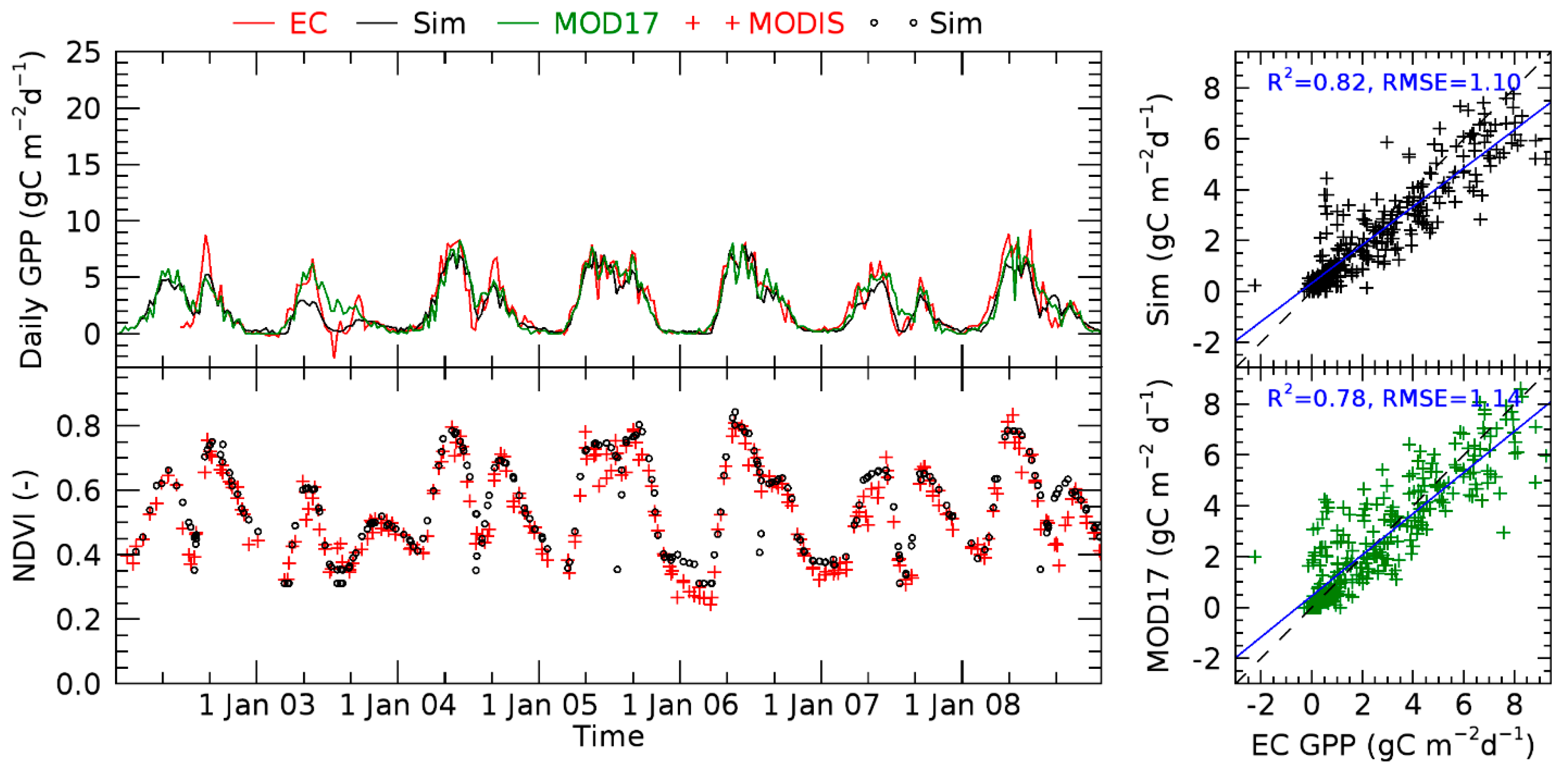
Figure 5.
Observed and modelled GPP and NDVI for the grassland site At-Neu. Description of plots as Figure 2.
Figure 5.
Observed and modelled GPP and NDVI for the grassland site At-Neu. Description of plots as Figure 2.
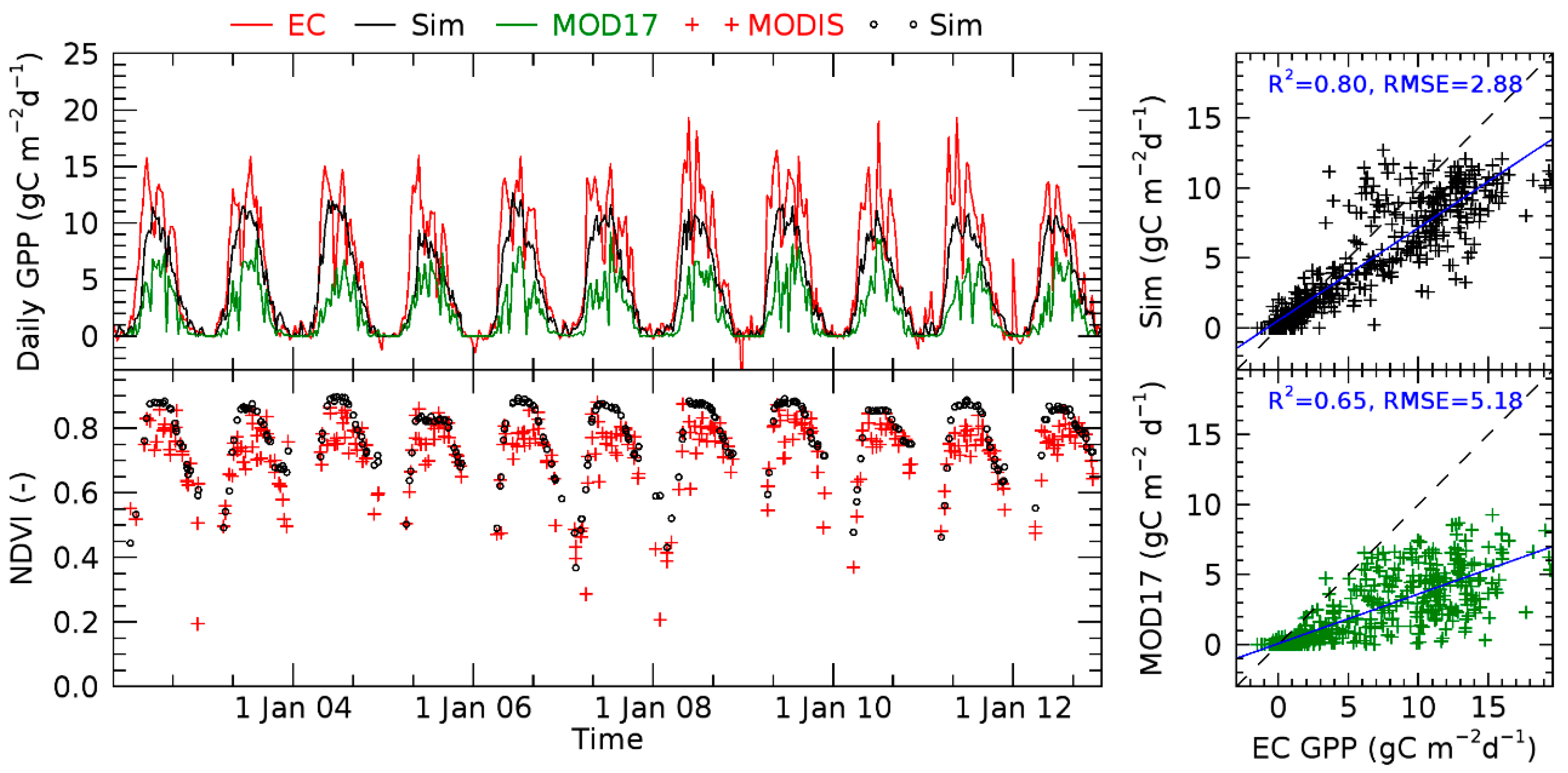
Figure 6.
Observed and modelled GPP and NDVI for the grassland site IT-Amp. Description of plots as Figure 2.
Figure 6.
Observed and modelled GPP and NDVI for the grassland site IT-Amp. Description of plots as Figure 2.
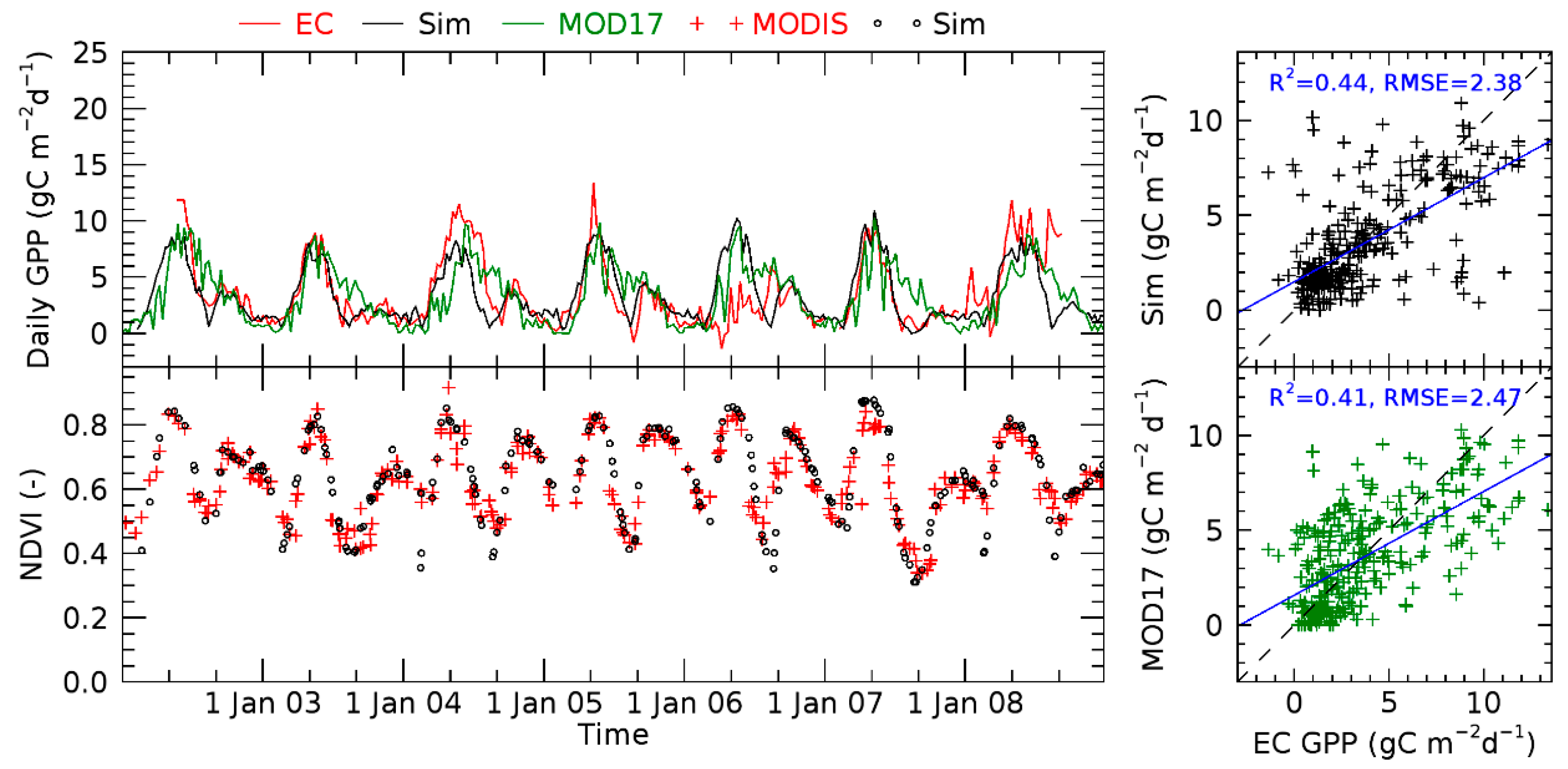
Figure 7.
Scatter plots of EC GPP versus GPP estimated by the Sim model for all sites (A), crop sites (B), and grassland sites (C). The dashed line is the 1:1 line while the continuous line is the ordinary least square linear regression. The following statistics are reported: coefficient of determination (R2), Perason’s correlation coefficient (r), p-value of the linear regression, gain and offset of the linear regression line, Root Mean Square Error (RMSE), Mean Bias Error (MBE), and total number of data points (n).
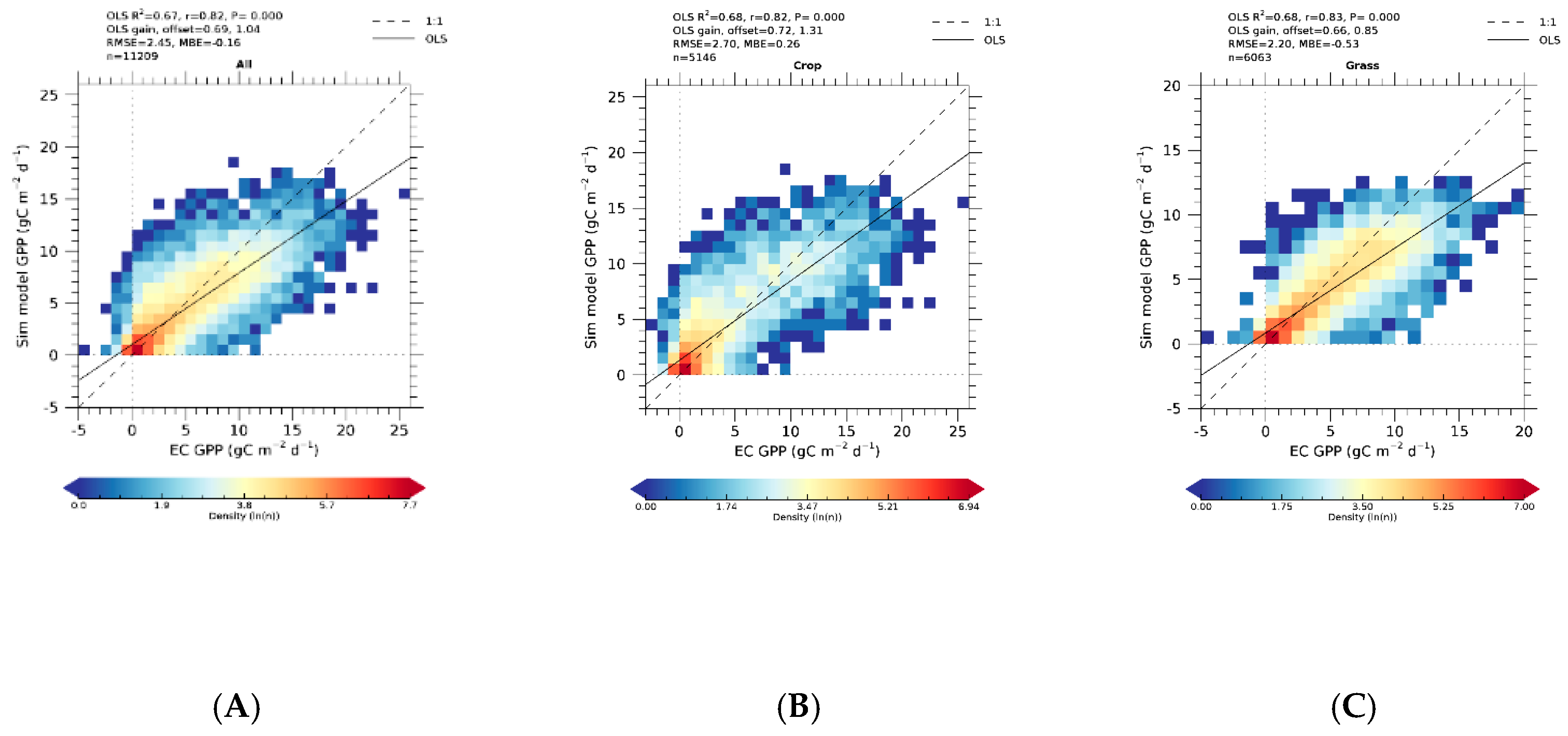
Figure 8.
Scatter plots of EC GPP vs. GPP estimated by MOD17 for all sites (A), crop sites (B), and grassland sites (C). Description of plots as Figure 7.
Figure 8.
Scatter plots of EC GPP vs. GPP estimated by MOD17 for all sites (A), crop sites (B), and grassland sites (C). Description of plots as Figure 7.
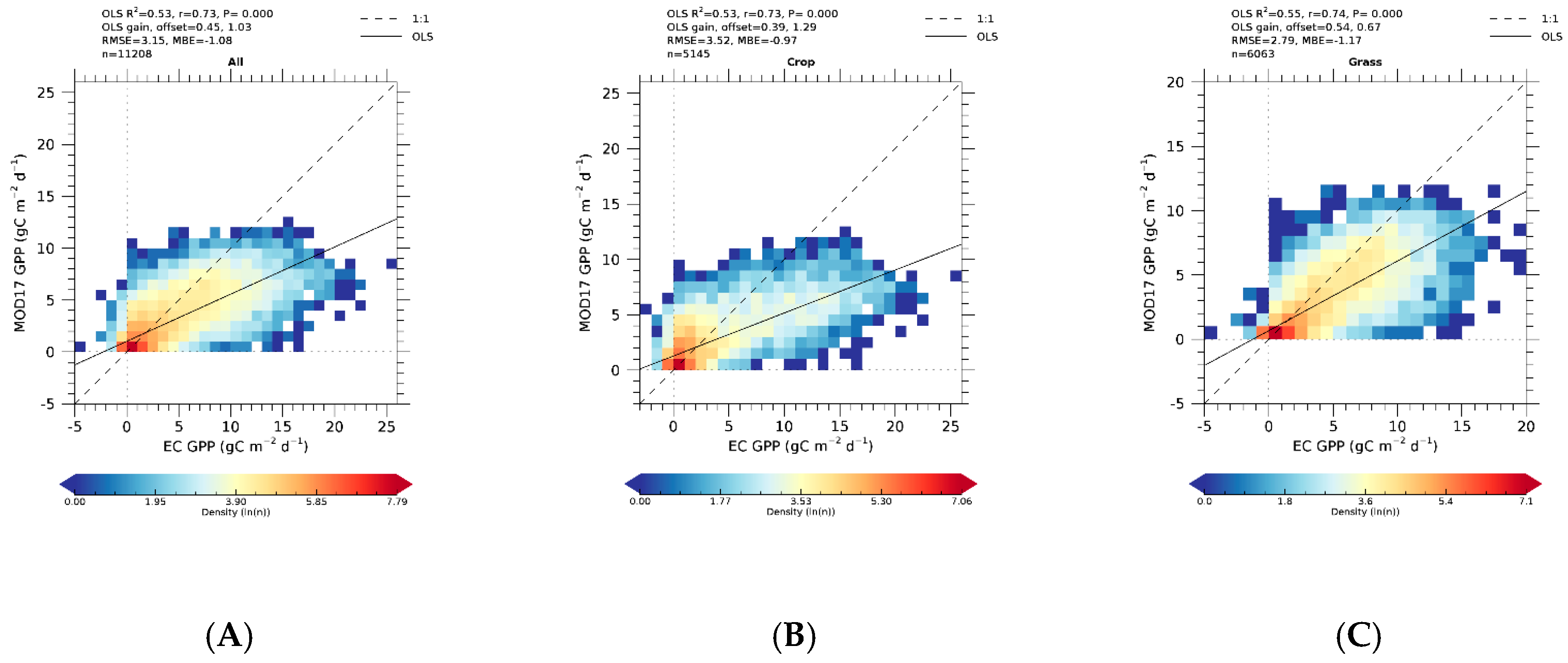
Figure 9.
Scatter plots of annual GPP: EC GPP versus GPP estimated by the Sim model (left) and MOD17 (right). Circle and triangle symbols denote crop and grassland sites, respectively. Symbol color ranges from red to blue and indicated the site latitude. Crop symbols with green circle outline highlight site-year data points referring to maize. The dashed line is the 1:1 line while the continuous line is the ordinary least square linear regression. The coefficient of determination (R2), the Root Mean Square Error (RMSE), Mean Bias Error (MBE), and the number of data points (n) are reported for all sites together, only crop sites and only grassland sites. Incomplete years (with partial EC measurements temporal cover) were excluded from this analysis.
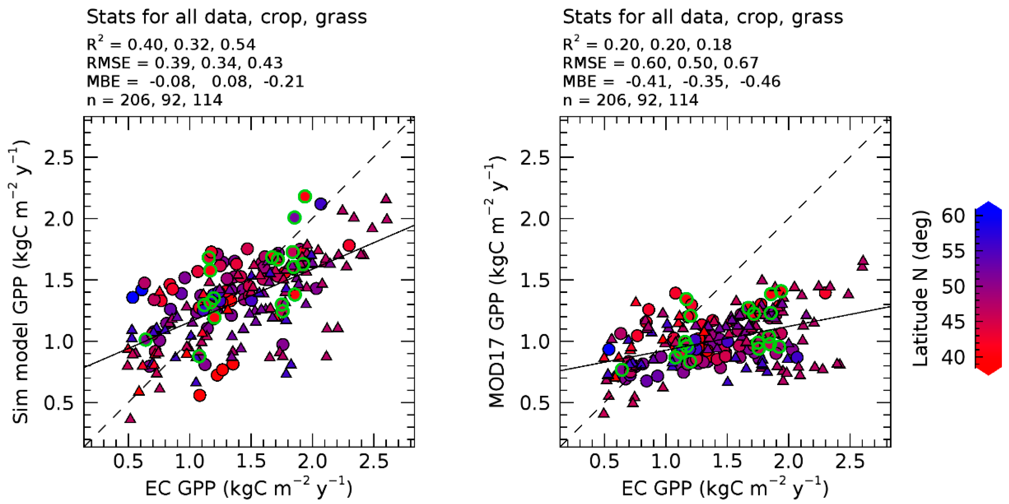
Figure 10.
Scatter plots of mean annual GPP per site: EC GPP versus GPP estimated by the Sim model (left) and MOD17 (right). Description of plots as Figure 9. Incomplete years (with partial EC measurements temporal cover) were excluded from this analysis. As a result, a subsample of 45 sites having at least one complete year was available.

Figure 11.
Histograms of the site-level Pearson correlation coefficient (r) between EC and modelled annual GPP for the Sim model (top row) and MOD17 (bottom row). Distribution of r for all sites (left column), crop sites (central column), and grassland sites (right column). Incomplete years (with partial EC measurements temporal cover) were excluded from this analysis. The site-level correlation was computed only when at least four years were available (average, minimum, and maximum years per site is 6, 4 and 11).

Table 1.
Data used in the analysis. ECMWF stands for European Centre for Medium-Range Weather Forecasts; MODIS: Moderate Resolution Imaging Spectroradiometer; NVDI: Normalized Difference Vegetation Index; GPP: gross primary production.
Table 1.
Data used in the analysis. ECMWF stands for European Centre for Medium-Range Weather Forecasts; MODIS: Moderate Resolution Imaging Spectroradiometer; NVDI: Normalized Difference Vegetation Index; GPP: gross primary production.
| Variable | Source | Main Specifications | Purpose |
|---|---|---|---|
| Global radiation, air temperature, precipitation, reference potential evapotranspiration | Downscaled ECMWF ERA-Interim, available from MARSOP repository 1 | Daily data, 25 km spatial resolution | Model input |
| NDVI | MODIS 2 | MOD- and MYD-13Q1, 16 day composites, 250 m spatial resolution | Model re-calibration |
| Surface reflectance | MODIS 2 | MOD- and MYD-09A, 8 day composites, 500 m spatial resolution | Estimation of canopy background reflectance |
| GPP | Eddy flux tower 3 | Daily data | GPP validation |
| GPP | MODIS 2 | MOD17A2H, 8 day composites, 500 m spatial resolution | GPP estimates intercomparison |
1https://marswiki.jrc.ec.europa.eu/agri4castwiki/index.php/Welcome_to_WikiMCYFS. 2 Data retrieved through the Google Earth Engine. 3 From European Flux Database Cluster and FLUXNET2015.
Table 2.
PROSAIL5B fixed parameters values.
| Variable | Value |
|---|---|
| Cab, Leaf chlorophyll content | 30 µg cm−2 |
| Cw, leaf equivalent water thickness | 0.015 g cm−2 |
| Ns, leaf structure coefficient | 1.6 (-) |
| Lidf_a and Lidf_b describing leaf angle distribution | −035, −01.15 (spherical distribution) |
| Hot spot size parameter | 0.5 |
Table 3.
Model parameters subject to optimization. LSP stands for Land Surface Phenology, the satellite-based phenological timings described in Section 3.3. FG stands for first guess.
Table 3.
Model parameters subject to optimization. LSP stands for Land Surface Phenology, the satellite-based phenological timings described in Section 3.3. FG stands for first guess.
| Variable | Units | Description | First Guess | Range | Reference |
|---|---|---|---|---|---|
| DOY0 | Day of year | Day at which the simulation starts and LAI is set to LAI0, i.e., the “emergence” date. | LSP | ±60 days | - |
| LAI0 | m2m−2 | Leaf area index at DOY0 | 0.02 | 0.01–0.08 | - |
| SLA | m2g−1 | Specific Leaf Area | 0.012 | 0.002–0.025 | [52,53,54,55] |
| c | GDD | Leaf lifespan offset Equation (5) | Multi-annual average of GDD from SOS to TOM | 250-FG * 1.5 | - |
| d | - | Leaf lifespan gain Equation (5) | 0.0 | 0–3 | [14] |
| Plmax | - | Maximum leaf partitioning ratio Equation (6) | 0.3 | 0.1–0.8 | [56] |
| GDDmax | GDD | GDD from emergence after which no partitioning to leaves occur Equation (8) | Same as parameter c | - | |
Table 4.
Summary statistics of GPP estimation performances. R2, RMSE, and MBE are derived from the scatter plots of Figure 7 and Figure 8 and represent the coefficient of determination of the ordinary least square linear regression, the Root Mean Square Error and the Mean Bias Error, respectively. The percent variation refers to the statistic of the Sim model as compared to that of MOD17. * The percent variation on MBE is computed on absolute values.
| Modelled vs. Observed | |||||||||
|---|---|---|---|---|---|---|---|---|---|
| All sites | Crops | Grasslands | |||||||
| Model | R2 | RMSE | MBE | R2 | RMSE | MBE | R2 | RMSE | MBE |
| MOD17 | 0.53 | 3.15 | −1.08 | 0.53 | 3.52 | −0.97 | 0.55 | 2.79 | −1.17 |
| Sim model | 0.67 | 2.45 | −0.16 | 0.68 | 2.70 | 0.26 | 0.68 | 2.20 | −0.53 |
| %variation | +26.42 | −22.2 | −85.19 * | +28.3 | −23.3 | −73.2 * | +23.64 | −21.2 | −54.7 * |
© 2019 by the authors. Licensee MDPI, Basel, Switzerland. This article is an open access article distributed under the terms and conditions of the Creative Commons Attribution (CC BY) license (http://creativecommons.org/licenses/by/4.0/).
Share and Cite
MDPI and ACS Style
Meroni, M.; Fasbender, D.; Lopez-Lozano, R.; Migliavacca, M. Assimilation of Earth Observation Data Over Cropland and Grassland Sites into a Simple GPP Model. Remote Sens. 2019, 11, 749. https://doi.org/10.3390/rs11070749
AMA Style
Meroni M, Fasbender D, Lopez-Lozano R, Migliavacca M. Assimilation of Earth Observation Data Over Cropland and Grassland Sites into a Simple GPP Model. Remote Sensing. 2019; 11(7):749. https://doi.org/10.3390/rs11070749
Chicago/Turabian StyleMeroni, Michele, Dominique Fasbender, Raul Lopez-Lozano, and Mirco Migliavacca. 2019. "Assimilation of Earth Observation Data Over Cropland and Grassland Sites into a Simple GPP Model" Remote Sensing 11, no. 7: 749. https://doi.org/10.3390/rs11070749
Note that from the first issue of 2016, this journal uses article numbers instead of page numbers. See further details here.