Article

An Analysis of the Early Regeneration of Mangrove Forests using Landsat Time Series in the Matang Mangrove Forest Reserve, Peninsular Malaysia

by
Viviana Otero
1,*,
Ruben Van De Kerchove
2,
Behara Satyanarayana
3,
Husain Mohd-Lokman
3,
Richard Lucas
4,5,† and
Farid Dahdouh-Guebas
1,6,†
1
Systems Ecology and Resource Management Laboratory, Université Libre de Bruxelles (ULB), 1050 Brussels, Belgium
2
Vlaamse Instelling Voor Technologisch Onderzoek (VITO) Research Organisation, 2400 Mol, Belgium
3
Mangrove Research Unit, Institute of Oceanography and Environment, Universiti Malaysia Terengganu (UMT), 21030 Kuala Terengganu, Malaysia
4
Earth Observation and Ecosystem Dynamics Research Group, Aberystwyth University, Aberystwyth SY23 3DB, UK
5
School of Biological, Earth and Environmental Sciences, University of New South Wales (UNSW), Sydney 2052, Australia
6
Laboratory of Plant Biology and Nature Management, Vrije Universiteit Brussel (VUB), 1050 Brussels, Belgium
*
Author to whom correspondence should be addressed.
These authors contributed equally to this work.
Remote Sens. 2019, 11(7), 774; https://doi.org/10.3390/rs11070774
Submission received: 26 February 2019 / Revised: 19 March 2019 / Accepted: 26 March 2019 / Published: 31 March 2019
(This article belongs to the Special Issue Remote Sensing of Mangroves)

Abstract

:
Time series of satellite sensor data have been used to quantify mangrove cover changes at regional and global levels. Although mangrove forests have been monitored using remote sensing techniques, the use of time series to quantify the regeneration of these forests still remains limited. In this study, we focus on the Matang Mangrove Forest Reserve (MMFR) located in Peninsular Malaysia, which has been under silvicultural management since 1902 and provided the opportunity to investigate the use of Landsat annual time series (1988–2015) for (i) detecting clear-felling events that take place in the reserve as part of the local management, and (ii) tracing back and quantifying the early regeneration of mangrove forest patches after clear-felling. Clear-felling events were detected for each year using the Normalized Difference Moisture Index (NDMI) derived from single date (cloud-free) or multi-date composites of Landsat sensor data. From this series, we found that the average period for the NDMI to recover to values observed prior to the clear-felling event between 1988 and 2015 was 5.9 ± 2.7 years. The maps created in this study can be used to guide the replantation strategies, the clear-felling planning, and the management and monitoring activities of the MMFR.

Graphical Abstract

1. Introduction

Mangrove forests are woody plants found in the intertidal zones in tropical and subtropical latitudes [1,2]. As such, mangroves are subjected daily to changes in temperature, exposure to water and salt, and different degrees of hypoxia [3]. Mangroves have adapted to these changing conditions and are resilient ecosystems that can additionally cope with environmental changes and disturbances such as storms, hurricanes, mean sea-level fluctuations and climate variability [3]. In areas where conditions have remained relatively stable, mangroves have thrived and natural cycles of succession have prevailed [4,5].
Mangrove restoration and reforestation has garnered interest in recent years due to the carbon sequestration capacity of these forests [6,7]. Silviculture is one of the oldest reasons, among others, to pursue mangrove restoration projects [4,5]. Mangrove reserves such as the Matang Mangrove Forest Reserve (MMFR) in Malaysia, Bintuni Bay Mangroves in West Papua, Indonesia, and the Sundarbans in Bangladesh are examples of mangrove forests that are under silvicultural management [8,9,10]. In these cases of silvicultural management, restoration and reforestation of mangrove forests, it is essential to understand the conditions that favor mangrove propagule dispersal and establishment, mangrove growth and succession, and carbon sequestration.
Remote sensing has been frequently used to monitor changes in mangrove forest cover at local and global levels, e.g., [11,12,13,14,15,16,17,18,19,20,21,22,23]. With an increasing array and availability of satellite sensor data, there is an opportunity to routinely observe mangrove forests and support silvicultural management, restoration and reforestation projects. Using optical data, focus has often been on the use of spectral vegetation indices, such as Normalised Difference Vegetation Index (NDVI), to detect forest disturbances [24,25]. However, indices that exploit the short wave infrared (SWIR) spectra, such as the Normalised Difference Moisture Index (NDMI), have been found to be more effective than the NDVI in detecting forest disturbances [20,26,27,28]. The use of the SWIR reflectance can provide information about vegetation moisture content and about the upper canopy structure [29]. Moreover, temporal changes in these vegetation indices after a forest disturbance can also be used to detect forest recovery [20,25,26,30].
Studies on time series analysis have the potential to provide information of the past and current changes of mangrove forests [31,32,33,34,35,36,37]. Time series based on vegetation indices have been used to analyse changes in mangrove cover and phenology [32,33,36]. Nevertheless, the use of these types of time series to quantify the mangrove forest recovery after disturbances is still limited [32,33,35]. In this study, we focused on the MMFR located in Peninsular Malaysia, as this reserve is silviculturally managed and provides a unique opportunity to establish whether (i) time series of Landsat sensor data could be used to detect the clear-felling events that regularly take place in the reserve, and (ii) the NDMI annual time series could be used to trace back and quantify the early recovery of mangrove forest patches after a clear-felling event.

2. Materials and Methods

2.1. Study Area and Silvicultural Management

The MMFR has been under management since 1902 for charcoal and pole production [38]. The reserve is a riverine mangrove forest comprising 27 mangrove species [8]. The reserve has an area of 40288 ha and is divided in four different administrative zones: Protective (17.4% of the reserve’s total forest area), productive (74.8%), restrictive productive (6.8%) and unproductive (1%) (Figure 1) [8]. The productive and restrictive productive zones are under silvicultural management and are the only areas where the wood extraction occurs. They are composed of forests dominated primarily by Rhizophora apiculata Blume and R. mucronata Lamk. The silvicultural management consists of a 30-year rotation cycle with two thinnings at 15 and 20 years after clear-felling [8]. The protective zones are composed of diverse mangrove genera such as Avicennia, Sonneratia, Bruguiera and Rhizophora. Patches of dryland forest exist within the protective zones. The reserve provides ecosystem services, including provision of wood for charcoal and pole production, coastal protection, conservation of flora and fauna, and mangrove propagule production [8]. The unproductive zones are represented by lakes and infrastructure areas, including villages, charcoal kilns and administrative buildings [8].
The reserve is located in the west coast of Peninsular Malaysia (Figure 1). The reserve has a tropical climate, with an average air temperature ranging from 22 °C at night to 33 °C during the day [8]. Relative humidity ranges from 99% in the early morning to 60% around noon [40]. Peninsular Malaysia has monsoon season between November and March, and between May and September [41]. The annual rainfall ranges from 2000 mm to 2800 mm [8]. The area is subjected to semidiurnal tides and the tidal amplitude range is 3.3 m [42]. Freshwater flows into the reserve via streams and ground run-off [42].
Every ten years the local management defines the management plan for the reserve [8]. During the period of analysis of this study four different management plans have been developed: 1980 to 1989, 1990 to 1999, 2000 to 2009, and 2010 to 2019 [8,40]. It is noteworthy that the silvicultural practice of a 30-year rotation cycle with two thinnings at 15 and 20 years after clear-felling has remained constant for each plan. Within each management plan, areas to be clear-felled or thinned are pre-assigned and are further divided into smaller areas, called coupes (areas between 2.2 and 6.6 ha), which are then allocated to approved charcoal contractors [8]. Clear-felling activities are performed every year by different contractors, but a coupe will only be clear-felled once every 30 years [8].

2.2. Methods

We followed the workflow outlined in Figure 2 to detect the clear-felling events in the MMFR and quantify the early regeneration of mangroves within the logging coupes. Specifically, Landsat data for the period 1988 to 2015 were used to generate a single cloud-free image or a multi-date composite for each year (28 in total). Based on these data, the single Normalised Difference Moisture Index (NDMI) and Normalised Difference Vegetation Index (NDVI) layers were derived. The NDMI time series was found to be optimal to map the extent of clear-felling events and the early regeneration of mangrove forests within coupes. The resulting extent and regeneration maps (i.e., clear-felling and recovery time) were validated against local management plans and a dataset of 135 reference time series. The following sections provide a summary of the processing undertaken.

2.2.1. Satellite Imagery

Landsat Thematic Mapper (TM), Enhanced Thematic Mapper Plus (ETM+) and Operational Land Imager (OLI) acquired over the period 1988 to 2015 were used to create the time series of the MMFR (Table 1). Surface reflectance Level 2 data products were downloaded from the United States Geological Survey (USGS) Earth Explorer site [43,44]. The surface reflectance data products from TM and ETM+ were generated using the Landsat Ecosystem Disturbance Adaptive Processing System (LEDAPS) software [45] implemented by USGS [43]. The surface reflectance products from OLI were generated using the Landsat 8 Surface Reflectance Code (LaSRC) algorithm [46] implemented by USGS [44]. The surface reflectance Level 2 data products are already radiometrically and atmospherically corrected [45,46].

2.2.2. Time Series Creation

For each year from 1988 to 2015, an annual surface reflectance image was generated from individual cloud-free scenes or composites of the several scenes within one year. Only one image was used for each year, given that logging coupes are typically cleared over a two-year period and only once every 30 years. To create a multi-date composite image for each year with prevalent cloud cover, we first selected the image with the least amount of clouds and cloud shadow. Where the land surface was obscured, we replaced affected areas with the pixel values from another image of the same year. On average, we only had to replace values in 3 % of data contained in the image with the least amount of cloud cover from 1988 to 2015. The final image was comprised of data from several dates but this was considered acceptable given that clear-felling takes place over an extended period and is not seasonally dependent. The final data stack consisted of 28 images, with each band representing the surface reflectance of a single year. Two additional image stacks representing the NDVI and NDMI (Equations (1) and (2)) for each year were also generated from 1988 to 2015 based on the surface reflectance [29,47]:
NDVI = (NIR − R)/(NIR + R),
NDMI = (NIR − SWIR)/(NIR + SWIR),
where NIR is the Near-Infrared band, R is the red band and SWIR is the short-wave infrared band. In the event of a missing value for a pixel due to cloud cover, the NDVI and NDMI values for the corresponding pixel were interpolated based on the pixel’s NDVI and NDMI values from the previous and following year. We only encounter this problem for 2012, where 70% of the image was missing due to a failure in the Scan Line Corrector (SLC) of Landsat 7 [48].

2.2.3. Fieldwork

We acquired Unmanned Aerial Vehicle (UAV) imagery in different forests stands between June and July 2016. We collected data on four different types of forests: A stand that was clear-felled between the end of 2015 and beginning 2016, and stands of 7, 14 and 30 years in age. UAV data were acquired using a DJI Phantom 3 Professional quadcopter UAV and the in-built true color camera, and used to create four orthomosaics of 1ha for each type of forest stand [49].

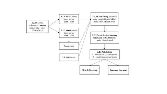
2.2.4. Time Series Analysis

Using the NDVI annual time series, we created a water mask for the MMFR, which includes all areas of open water in the ocean, rivers, creeks and non-vegetated inundated mudflats. If the NDVI value was zero or negative at any point in the time series, the corresponding pixel was classified as water throughout as this approach accounted for different water levels. Areas classified as water were excluded from further analysis. Additionally, areas of non-vegetated terrestrial land covers (i.e., urban infrastructure and dry soils) were associated with pixels with a negative NDMI value and were also excluded. Finally, we excluded land areas located outside the reserve based on the management zones map (Figure 1).
Within the remaining area, we detected the clear-felling events using the NDMI time series. We evaluated 210785 time series of pixels from 1988 to 2015. For each series of pixels, we evaluated the following cases:
  • We detected clear-felling events based on two conditions:
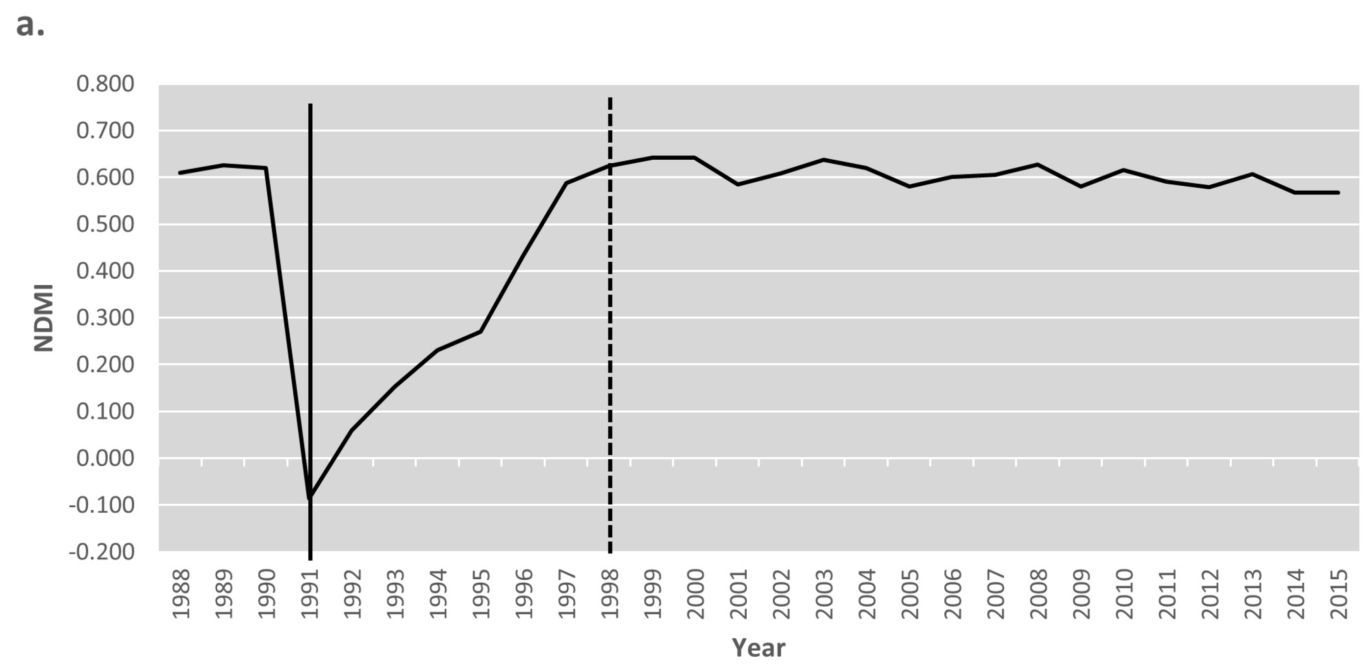
    • We first defined a reference year as the year when the NDMI was below 0.288. This threshold was determined through comparison of the NDMI series of pixels associated with clear-felled and non-clear-felled areas. Areas with dense vegetation (including pre-logged and mature mangroves) exhibited NDMI values around 0.5, which contrasted with areas that were clear-felled which exhibited NDMI values below 0.288.
    • The difference between the NDMI of the reference year and the following year was at least 0.275. We defined this second threshold to guarantee that the drop in the NDMI value was sufficient to correspond to a true clear-felling event. This second threshold was also determined by comparing different series of pixels associated with clear-felled and non-clear-felled areas. The approach followed on from previous studies [30,50,51,52] that have also used thresholds to analyse time series.
  • We determined the following values for each clear-felling event:
    • The year of clear-felling
    • The year of recovery. This value was determined as the year when the NDMI value returned to the state prior to clearing [26]. This previous state was defined as the median value of all the points in the series before the clear-felling event minus one standard deviation to account for normal fluctuations in the vegetation index.
    • The recovery time. This time is defined as the number of years that the mangrove forest took to regenerate that is, the difference between the year of recovery and the year of the clear-felling occurrence. If this number was one, we considered this event as noise as mangrove regeneration is not possible in a single year.
    • The drop in the NDMI value, calculated as the difference between the NDMI value before clear-felling and the lowest NDMI value in the time series.
It was not possible to determine the recovery time for clear-felling events that had not restored to pre-clearance levels by 2015. Such areas were typically cleared after 2009 and the forests did not appear to have had enough time to regenerate. Additionally, we did not calculate the recovery time in areas that were already clear-felled in 1988 as there was no knowledge as to whether clearing had occurred in or prior to that year.
We recorded the information of the clear-felling events in five maps describing per pixel: (a) The year of clear-felling or the absence of clear-felling, (b) the recovery time after clear-felling (c) the drop in the NDMI value, (d) whether clear-felling occurred between 1988 and 2015 without complete regeneration by 2015, and finally (e) the extend of water throughout the period of the time series based on the NDVI time series. All these maps were created using the RStudio version 1.1.456, R version 3.4.1 using the raster and rgdal packages [53].

2.2.5. Validation Time Series Analysis

We validated our clear-felling maps by comparing them visually against:
  • The time series of 135 randomly selected pixels from locations clear-felled between 1989 and 2015. For each pixel, we determined the year of clear-felling and the recovery time by visual interpretation of the NDMI time series. We selected these points such that we included five examples of clear-felling events per year in the time series (from 1988 to 2015).
  • The management zone maps and the logging plans included in the management plans from 2000 to 2009, and 2010 to 2019 [8,40]. First, we compared the existing local management zone map against the results of our clear-felling map, on the assumption that clearing only occurs in the productive and restrictive productive areas (i.e., where wood extraction is officially approved). Second, we compared the clear-felling year calculated in this study against the logging plans outlined in those management plans. These logging plans contain the year when the coupes should be clear-felled.

3. Results

3.1. Time Series Creation

Water areas were more easily discriminated using the NDVI time series as compared to the NDMI time series. Water areas exhibited a negative NDVI value as compared to vegetated areas that had a positive NDVI value (Figure 3b,d). The NDMI provided a measure of the moisture content in both vegetated areas and water (Figure 3a,c) and therefore exhibited similar positive values for both. The NDVI annual time series was therefore used to discriminate water bodies from vegetated areas (see supplementary data Figure S1).
The rapid decrease in the NDMI following clear-felling is highlighted in Figure 4a, with values considerably lower than forests that were not clear-felled between 1988 and 2015 (Figure 4c). The NDMI declines primarily because of the reduction in vegetation amount (and hence structural complexity) and exposure of the underlying surface. The lowest value in the NDMI time series was attained once all vegetation had been completely removed from a clear-felled area, which typically occurred within two years following the clear-felling event [8]. Differences in the NDMI between pre- and post-clear-felling were greater compared to the NDVI (Figure 4b), therefore providing better detection of clear-felled areas. Additionally, we used the NDMI time series to detect urban areas in order to exclude them from our analysis (see supplementary data Figure S2).

3.2. Reference to Field and UAV Data

The relationship between the changes in the NDMI time series and the forest structure observed on the field is illustrated in Figure 5. We observed a very closed canopy from seven-year-old to 30-year-old forests (Figure 5 UAV top view). The contrast with a recently clear-felled area is noticeable, where the remaining trunks and dried branches are still present in the area (Figure 5, Example 2). Moreover, the first signs of mangrove re-establishment are observed on the ground in the clear-felled areas, with some saplings already present (Figure 5, ground view Example 2). A view from the ground also confirms the high tree density in young forests of seven and 14-year-old stands (Figure 5 bottom images, Examples 3 and 4). Although older forests generally have a lower density of trees, the canopy is regarded as closed when viewed from above (Figure 5, Example 1). It is noteworthy that the forest structure prior to clearing is not the same after the NDMI reaches a value that is similar to that of the pre-cleared forests. Therefore, changes captured by the NDMI time series only reflect the early regeneration of the mangrove forests, as these forests will continue their growth further.

3.3. Time series Analysis

In Figure 6, two examples show the year of clear-felling and the year of recovery detected for the NDMI time series of two pixels.
The year of clear-felling for each Landsat pixel contained within the MMFR is given in Figure 7. Areas found to be clear-felled in the same year match the areas assigned for clear-felling by the local management (see Section 3.4). We detected clear-felling events in 88.4% (16,776 ha or 186,402 pixels) out of the 210,785 pixels analysed between 1989 and 2015. The median clear-felled area per year was 600 ± 242 ha.
The mean recovery time (i.e., the period for NDMI values to return to pre-clearance values), taking into account all the clear-felling events that recovered by 2015, was 5.87 ± 2.67 years (Figure 8). The median recovery time (interquartile range) was five years (4–7 years) and the minimum and maximum was two and 25 years respectively. It is noteworthy that recovery times were uneven across coupes clear-felled in the same year (Figure 8b,c).

3.4. Validation Time Series Analysis

Comparison with the 135 reference points (Section 2.2.5) indicated that 100% were correctly identified as clear-felled in the corresponding year and 96% determined the same recovery time as the time defined by visual inspection. Incorrect matching of the remaining 4% (five points) was attributed to noisy data (e.g., a sudden increase or decrease in the signal before the occurrence of the clear-felling, see supplementary data Figure S4) and limited information available on the previous state (clearance history). In these cases, the algorithm overestimated the recovery time by one year in two cases, underestimated by two years in another two cases, and underestimated by five years in one case. In this last case the signal was noisy and defining the recovery time was not straightforward even through visual interpretation (see supplementary data Figure S4).
Reference to the pre-existing forest management maps (Figure 1) established that clear-felling events had taken place in the productive and restrictive productive zones. We also identified changes in three areas that are protective zones according to the management plan but these changes require further investigation to determine the actual cause of change (Supplementary data Figure S5). Furthermore, we compared the map of the year of clear-felling with the management plan map that prescribes the year when the coupes should be clear-felled. The coupes designated by the local management plan emerge in the map of the year of clear-felling created in this study (see Figure 9). However, the clear-felling events detected in this study occurred on average 2.85 ± 1.15 years after the planned year. It is noteworthy that the management plan is a scheme that is defined before the actual clear-felling. Therefore, the satellite imagery precisely indicates when the actual clear-felling took place (see supplementary data Table S1).

4. Discussion

4.1. Time Series Analysis

The NDMI time series could be used to detect the clear-felling events and quantify the recovery time. These results are in accordance with the studies of DeVries et al. [26], Kennedy et al. [20], Jin and Sader [28] and Wilson and Sader [27] which also found that the NDMI time series are useful for detecting forest changes, disturbances and regeneration. The NDMI is indicative of the moisture content and structural complexity of forests and therefore vegetated areas and water have a positive value. Following clear-felling, the NDMI decreases rapidly as vegetation is removed and the soil is exposed. However, the forests regenerate (with assistance from planting) and the NDMI values return to those typical of the pre-cleared forest and remain similar until the next clearing event. Hence, only the first years of regeneration can be quantified as the NDMI saturates in dense vegetation [54,55,56] despite differences in forest structure. Nevertheless, we were able to identify variations in the recovery times between and within the management-defined coupes.
To the best of our knowledge, this is the first study that quantifies early forest recovery times in the MMFR using annual Landsat time series. Previous studies on mangrove regeneration have focused on quantifying new mangrove cover [32,33]. Although knowledge of new areas colonized by mangrove is certainly important and required to improve the management of mangrove areas, measurements other than area are required to quantify mangrove regeneration in the MMFR. Aziz et al. [57] used nine Landsat satellite images from 1978 to 2014 to analyse mangrove regeneration in the MMFR by classifying the forests as young or mature. Nevertheless, they did not use annual time series nor did they quantify recovery times.
This study generated maps of clear-felling that mirrored the coupes defined by the local management, albeit with some minor differences in the shapes of coupes. This corroborates the findings of this study and opens the possibility for using the methods introduced here to support local management of the MMFR. Clear-felling events were detected on a pixel-by-pixel basis and hence, if one pixel was partially clear-felled and some vegetation still remained within the pixel, it was not possible to detect the clear-felling event as there was an insufficient decrease in the NDMI. This case can occur as the management suggests that about eighteen mature Rhizophora trees should be retained per hectare in the clear-felled areas to serve as a propagule source for recolonization [8]. However, this limitation does not hinder the usefulness of our maps to support the local management, as the area of each coupe is practically completely identified in this study. Overall, we confirm the results of Aziz et al. [57,58] highlighting the usefulness of the Landsat archive to support the local management of the MMFR.
We also identified changes in three protective zones (see supplementary data Figure S5), one of which was also studied by Aziz et al. [57]. We found possible changes in the forest structure captured by a sudden drop in the NDMI time series in areas where Avicennia-Sonneratia, Rhizophora and dryland forests are located. Whilst not in the productive zones, these changes highlight the vulnerability of the managed forest to events or processes that can have implications in the ecosystem services that the protective zones provide for the MMFR [4,57].
Mangrove recovery times were shown to vary from two to 25 years after clearing and also differed between and within areas that were clear-felled in the same year. Mangrove propagule dispersal and establishment are complex processes that are influenced by factors such as currents, water depth, wind, salinity, geomorphology, propagule predation, propagule morphology, light and nutrients availability [59,60,61,62,63,64]. Therefore, further studies are needed to explain the variations in the recovery time that take into account the aforementioned factors and increase our understanding of the drivers of mangrove regeneration.

4.2. Implication for the Local Management

The results of this study are new and useful for the local management of the MMFR. The management in the MMFR implements a policy of active replanting. Two years after a clear-felling event, the management assesses the cleared area and if the natural regeneration is less than 90%, Rhizophora seedlings are planted where needed [8]. This policy has an impact on the vegetation cover two years after clear-felling and therefore on the NDMI. The recovery times identified in this study extend beyond the two-year assessment period. Hence, this study can inform the local management on where and when to replant. This study can also identify where past planting might not have been as successful as anticipated and therefore can better inform on future management pathways.
Additionally, the results of this study can also be used to support monitoring activities, redefine current and new administrative forest zones, and guide the planning of clear-felling events. The identification of changes in the NDMI can also offer a view of changes that occur in both productive zones and protective zones. This information can be used to update current management maps and monitor the forests in the zones where wood extraction does not occur but nevertheless are relevant for maintaining ecosystems services in the reserve, such as propagule source, coastal protection and protection of flora and fauna [8]. Moreover, the availability of free satellite imagery opens the possibility to increase the frequency of the monitoring as mangrove areas are difficult to access [49].
The methodology used in this study can also be used in other mangrove areas that are under silvicultural management such as Bintuni Bay in West Papua, Indonesia [9] and the Sundarbans [10]. Bintuni Bay has a silvicultural management focused on Rhizophora species with a rotation cycle of 25 years and a similar replantation strategy as the one used in MMFR [9]. Therefore, the methodology proposed in this study could also be used by the management of this mangrove area in West Papua. Furthermore, the mangrove areas that are not under silvicultural management could benefit from using the NDMI time series to detect disturbances in forest structure. As recently outlined by Curnick et al. [65] even the smallest patches of mangroves threatened by anthropogenic disturbance serve important ecosystem functions, goods and services and may benefit from early detection when disturbed. As we show in this study, these types of time series have the potential to detect disturbances and regrowth in already existing mangrove areas. Although a modification of the current methodology would be necessary to consider the drivers of other types of disturbances, the potential to track regrowth after a disturbance is useful for mangrove conservation and management worldwide.

5. Conclusions

This study confirmed that clear-felling events and early regeneration of mangrove forests in the MMFR could be quantified by means of Landsat time series. The NDMI was most useful for detecting clear-felling events that regularly take place in the reserve as part of the local management strategy. Additionally, the NDMI was useful to calculate the early regeneration of mangrove forests, with an average recovery time of 5.87 ± 2.67 years. The patterns of logging were similar to those outlined in the MMFR management plan. Therefore, the mapping provided by this study provides new insights into the recovery of mangrove forests in the MMFR and are a valuable approach to guide future clear-felling management, replanting strategies and monitoring.

Supplementary Materials

The following are available online at https://www.mdpi.com/2072-4292/11/7/774/s1; Figure S1: Water mask; Figure S2: NDMI and NDVI time series for urban areas; Figure S3: Time series analysis: NDMI drop calculation; Figure S4: Validation time series analysis by means of comparison with point dataset; Figure S5: Validation time series analysis by means of comparison with the management zones map; Table S1: Time series analysis validation by means of comparison with the clear-felling planning.

Author Contributions

Conceptualization, V.O., R.V.D.K., R.L. and F.D.-G.; Data curation, R.V.D.K.; Formal analysis, V.O.; Funding acquisition, R.V.D.K., B.S., H.M.-L., R.L. and F.D.-G.; Investigation, V.O., R.V.D.K., B.S., R.L. and F.D.-G.; Project administration, V.O., R.V.D.K., B.S., R.L. and F.D.-G.; Resources, R.V.D.K., B.S., H.M.-L., R.L. and F.D.-G.; Supervision, R.V.D.K., B.S., R.L. and F.D.-G.; Validation, V.O., R.V.D.K., R.L. and F.D.-G.; Writing—original draft, V.O.; Writing—review & editing, V.O., R.V.D.K., B.S., R.L. and F.D.-G.

Funding

This research was funded by BELSPO (Belgian Science Policy Office) in the frame of the STEREO III Programme—Project Managing Mangrove Forests with Optical and Radar Environmental Satellites (MAMAFOREST) grant number SR/00/323.

Acknowledgments

We would like to thank the Perak State Forestry Department and the local rangers of the MMFR for their support during the fieldwork and for providing the management plans of the reserve. We would also like to thank Muhammad Amir Bin Fisol, Emilia Ashari and Columba Martínez-Espinosa, for their collaboration during fieldwork. This study was carried with the approval of the Perak State Forestry Department, Ipoh, Malaysia. Landsat Surface Reflectance products courtesy of the U.S. Geological Survey. This paper is published with the support of the Belgian University Foundation. Publié avec le concours de la Fondation Universitaire de Belgique.

Conflicts of Interest

The authors declare no conflict of interest.

References

  1. Mukherjee, N.; Sutherland, W.J.; Khan, M.N.I.; Berger, U.; Schmitz, N.; Dahdouh-Guebas, F.; Koedam, N. Using expert knowledge and modeling to define mangrove composition, functioning, and threats and estimate time frame of recovery. Ecol. Evol. 2014, 4, 2247–2262. [Google Scholar] [CrossRef] [PubMed]
  2. Duke, N.C.; Ball, M.C.; Ellison, J.C. Factors influencing biodiversity and distributional gradients in mangroves. Glob. Ecol. Biogeogr. Lett. 1998, 7, 27–47. [Google Scholar] [CrossRef]
  3. Alongi, D.M. Mangrove forests: Resilience, protection from tsunamis, and responses to global climate change. Estuar. Coast. Shelf Sci. 2008, 76, 1–13. [Google Scholar] [CrossRef]
  4. Ellison, A. Mangrove restoration: Do we know enough? Restor. Ecol. 2000, 8, 219–229. [Google Scholar] [CrossRef]
  5. Bosire, J.O.; Dahdouh-Guebas, F.; Walton, M.; Crona, B.I.; Lewis, R.R., III; Field, C.; Kairo, J.G.; Koedam, N. Functionality of restored mangroves: A review. Aquat. Bot. 2008, 89, 251–259. [Google Scholar] [CrossRef] [Green Version]
  6. Donato, D.C.; Kauffman, J.B.; Murdiyarso, D.; Kurnianto, S.; Stidham, M.; Kanninen, M. Mangroves among the most carbon-rich forest in the tropics. Nat. Geosci. 2011, 4, 293–297. [Google Scholar] [CrossRef]
  7. Alongi, D.M. Carbon sequestration in mangrove forests. Carbon Manag. 2012, 3, 313–322. [Google Scholar] [CrossRef]
  8. Ariffin, R.; Mustafa, N.M.S.N. A Working Plan for the Matang Mangrove Forest Reserve, 6th ed.; State Forestry Department of Perak: Ipoh, Malaysia, 2013; pp. 38–43, 53–56, 60–63, 195–207.
  9. Sillanpaa, M.; Vantellingen, J.; Friess, D.A. Vegetation regeneration in a sustainably harvested mangrove forest in West Papua, Indonesia. For. Ecol. Manag. 2017, 390, 137–146. [Google Scholar] [CrossRef]
  10. Iftekhar, M.S.; Islam, M.R. Managing mangroves in Bangladesh: A strategy analysis. J. Coast. Conserv. 2004, 10, 139–146. [Google Scholar] [CrossRef]
  11. Kuenzer, C.; Bluemel, A.; Gebhardt, S.; Quoc, T.V.; Dech, S. Remote Sensing of Mangrove Ecosystems: A Review. Remote Sens. 2011, 3, 878–928. [Google Scholar] [CrossRef] [Green Version]
  12. Lucas, R.M.; Mitchell, A.L.; Rosenqvist, A.; Proisy, C.; Melius, A.; Ticehurst, C. The potential of L-band SAR for quantifying mangrove characteristics and change: Case studies from the tropics. Aquat. Conserv. 2007, 17, 245–264. [Google Scholar] [CrossRef]
  13. Green, E.P.; Clark, C.D.; Mumby, P.J.; Edwards, A.J.; Ellis, A.C. Remote sensing techniques for mangrove mapping. Int. J. Remote Sens. 1998, 19, 935–956. [Google Scholar] [CrossRef] [Green Version]
  14. Giri, C.; Ochieng, E.; Tieszen, L.L.; Zhu, Z.; Singh, A.; Loveland, T.; Masek, J.; Duke, N. Status and distribution of mangrove forest of the world using earth observation satellite data. Glob. Ecol. Biogeogr. 2011, 20, 154–159. [Google Scholar] [CrossRef]
  15. Fatoyinbo, T.E.; Simard, M. Height and biomass of mangroves in Africa from ICESat/GLAS and SRTM. Int. J. Remote Sens. 2013, 34, 668–681. [Google Scholar] [CrossRef]
  16. Thomas, N.; Lucas, R.; Bunting, P.; Hardy, A.; Rosenqvist, A.; Simard, M. Distribution and drivers of global mangrove forest change, 1996-2010. PLoS ONE 2017, 12, e0179302. [Google Scholar] [CrossRef]
  17. Dahdouh-Guebas, F.; Verheyden, A.; De Genst, W.; Hettiarachchi, S.; Koedam, N. Four decade vegetation dynamics in Sri Lankan mangroves as detected from sequential aerial photography: A case study in Galle. Bull. Mar. Sci. 2000, 67, 741–759. [Google Scholar]
  18. Satyanarayana, B.; Muslim, A.M.; Horsali, N.A.; Zauki, N.A.; Otero, V.; Nadzri, M.I.; Ibrahim, S.; Husain, M.L.; Dahdouh-Guebas, F. Status of the undisturbed mangroves at Brunei Bay, East Malaysia: A preliminary assessment based on remote sensing and ground-truth observations. PeerJ 2018, 6, e4397. [Google Scholar] [CrossRef] [PubMed]
  19. Ruwaimana, M.; Satyanarayana, B.; Otero, V.; . Muslim, A.M.; Syafiq, A.M.; Ibrahim, S.; Raymaekers, D.; Koedam, N.; Dahdouh-Guebas, F. The advantages of using drones over space-borne imagery in the mapping of mangrove forests. PLoS ONE 2018, 13, e0200288. [Google Scholar] [CrossRef]
  20. Kennedy, R.E.; Yang, Z.; Cohen, W.E. Detecting trends in forest disturbance and recovery using yearly Landsat time series: 1. LandTrend-Temporal segmentation algorithms. Remote Sens. Environ. 2010, 114, 2897–2910. [Google Scholar] [CrossRef]
  21. Broich, M.; Hansen, M.C.; Potapov, P.; Adusei, B.; Lindquist, E.; Stehman, S.V. Time-series analysis of multi-resolution optical imagery for quantifying forest cover loss in Sumatra and Kalimantan, Indonesia. Int. J. Appl. Earth Obs. Geoinf. 2011, 13, 277–291. [Google Scholar] [CrossRef]
  22. Hansen, M.C.; Potapov, P.V.; Moore, R.; Hancher, M.; Turubanova, S.A.; Tyukavina, A.; Thau, D.; Stehman, S.V.; Goetz, S.J.; Loveland, T.R.; et al. High-Resolution Global Maps of 21st-Century Forest Cover Change. Science 2013, 342, 850–885. [Google Scholar] [CrossRef]
  23. Zhu, Z.; Woodcock, C.E. Continuous change detection and classification of land cover using all available Landsat data. Remote Sens. Environ. 2014, 144, 152–171. [Google Scholar] [CrossRef]
  24. Verbesselt, J.; Hyndman, R.; Zeileis, A.; Culvenor, D. Phenological change detection while accounting for abrupt and gradual trends in satellite image time series. Remote Sens. Environ. 2010, 114, 2970–2980. [Google Scholar] [CrossRef] [Green Version]
  25. Verbesselt, J.; Zeileis, A.; Herold, M. Near real-time disturbance detection using satellite image time series. Remote Sens. Environ. 2012, 123, 98–108. [Google Scholar] [CrossRef]
  26. DeVries, B.; Decuyper, M.; Verbesselt, J.; Zeileis, A.; Herold, M.; Joseph, S. Tracking disturbance-regrowth dynamics in tropical forests using structural change detection and Landsat time series. Remote Sens. Environ. 2015, 169, 320–334. [Google Scholar] [CrossRef]
  27. Wilson, E.H.; Sader, S. Detection of forest harvest type using multiple dates of Landsat TM imagery. Remote Sens. Environ. 2002, 80, 385–396. [Google Scholar] [CrossRef]
  28. Jin, S.; Sader, S.A. Comparison of time series tasselled cap wetness and the normalized difference moisture index in detecting forest disturbances. Remote Sens. Environ. 2005, 94, 364–372. [Google Scholar] [CrossRef]
  29. Gao, B. NDWI—A normalized difference water index for remote sensing of vegetation liquid water from space. Remote Sens. Environ. 1996, 58, 257–266. [Google Scholar] [CrossRef]
  30. Huang, C.; Goward, S.; Masek, J.G.; Thomas, N.; Zhu, Z.; Vogelmann, J.E. An automated approach for reconstructing recent forest disturbance history using dense Landsat time series stacks. Remote Sens. Environ. 2010, 114, 183–198. [Google Scholar] [CrossRef]
  31. Liu, M.; Zhang, H.; Lin, G.; Lin, H.; Tang, D. Zonation and directional dynamics of mangrove forests derived from time-series satellite imagery in Mai Po, Hong Kong. Sustainability 2018, 10, 1913. [Google Scholar] [CrossRef]
  32. Flores-Cardenas, F.; Millan-Aguilar, O.; Diaz-Lara, L.; Rodriguez-Arredondo, L.; Hurtado-Oliva, M.A.; Manzano-Sarabia, M. Trends in the Normalized Difference Vegetation Index for Mangrove Areas in Northwestern Mexico. J. Coast. Res. 2018, 34, 877–882. [Google Scholar] [CrossRef]
  33. Pastor-Guzman, J.; Dash, J.; Atkinson, P.M. Remote sensing of mangrove forest phenology and its environmental drivers. Remote Sens. Environ. 2018, 205, 71–84. [Google Scholar] [CrossRef]
  34. Proisy, C.; Viennois, G.; Sidik, F.; Andayani, A.; Enright, J.A.; Guitet, S.; Gusmawati, N.; Lemonnier, H.; Muthusankar, G.; Olagoke, A.; et al. Monitoring mangrove forests after aquaculture abandonment using time series of very high spatial resolution satellite images: A case study from the Perancak estuary, Bali, Indonesia. Mar. Pollut. Bull. 2018, 131, 61–71. [Google Scholar] [CrossRef] [PubMed] [Green Version]
  35. Lagomasino, D.; Fatoyinbo, T.; Lee, A.; Feliciano, E.; Trettin, C.; Shapiro, A.; Mangora, M.M. Measuring mangrove carbon loss and gain in deltas. Environ. Res. Lett. 2019, 14, 025002. [Google Scholar] [CrossRef]
  36. Brown, M.I.; Pearce, T.; Leon, J.; Sidle, R.; Wilson, R. Using remote sensing and traditional ecological knowledge (TEK) to understand mangrove change on the Maroochi River, Queensland, Australia. Appl. Geogr. 2018, 94, 71–83. [Google Scholar] [CrossRef]
  37. Zhai, L.; Zhang, B.; Roy, A.A.; Fuller, D.O.; Lobo Sternberg, L.S. Remote sensing of unhelpful resilience to sea level rise caused by mangrove expansion: A case study of islands in Florida Bay, USA. Ecol. Indic. 2019, 97, 51–58. [Google Scholar] [CrossRef]
  38. Chong, V.C. Sustainable utilization and management of mangrove ecosystems of Malaysia. Aquat. Ecosyst. Health Manag. 2006, 9, 249–260. [Google Scholar] [CrossRef]
  39. Weidmann, N.B.; Kuse, D.; Gleditsch, K.S. The Geography of the International System: The CShapes Dataset. Int. Interact. 2010, 36, 86–106. [Google Scholar] [CrossRef] [Green Version]
  40. Azahar, M.; Nik Mohd Shah, N.M. A Working Plan for the Matang Mangrove Forest Reserve, Perak: The Third 10-Year Period (2000–2009) of the Second Rotation, 5th ed.; State Forestry Department of Perak: Ipoh, Malaysia, 2003; pp. 250–261.
  41. Suhaila, J.; Jemain, A.A. Fitting daily rainfall amount in Malaysia using the normal transform distribution. J. Appl. Sci. 2007, 7, 1880–1886. [Google Scholar]
  42. Asthon, E.C.; Hogart, P.J.; Ormond, R. Breakdown of mangrove leaf litter in a managed mangrove forest in Peninsular Malaysia. Hydrobiologia 1999, 413, 77–88. [Google Scholar]
  43. USGS. Landsat 4–7 Surface Reflectance Code (LEDAPS) Product Guide; Version 1.0; USGS: Sioux Falls, SD, USA, 2018.
  44. USGS. Landsat 8 Surface Reflectance Code (LASRC) Product Guide; Version 1.0; USGS: Sioux Falls, SD, USA, 2018.
  45. Masek, J.G.; Vermote, E.F.; Saleous, N.E.; Wolfe, R.; Hall, F.G.; Huemmrich, K.F.; Gao, F.; Kutler, J.; Lim, T.-K. A Landsat surface reflectance dataset for North America, 1990–2000. IEEE Geosci. Remote Sens. Lett. 2006, 3, 68–72. [Google Scholar] [CrossRef]
  46. Vermote, E.; Justice, C.; Claverie, M.; Franch, B. Preliminary analysis of the performance of the Landsat 8/OLI land surface reflectance product. Remote Sens. Environ. 2016, 185, 46–56. [Google Scholar] [CrossRef]
  47. USGS. Product Guide: Landsat Surface Reflectance Derived Spectral Indices. Version 3.6. Available online: https://landsat.usgs.gov/sites/default/files/documents/si_product_guide.pdf (accessed on 11 January 2019).
  48. USGS. Preliminary Assessment of the Value of Landsat 7 ETM+ Data Following Scan Line Corrector Malfunction. Executive Summary. 16 July 2003. Available online: https://prd-wret.s3-us-west-2.amazonaws.com/assets/palladium/production/s3fs-public/atoms/files/SLC_off_Scientific_Usability.pdf (accessed on 14 January 2019).
  49. Otero, V.; Van De Kerchove, R.; Satyanarayana, B.; Martínez-Espinosa, C.; Bin Fisol, M.A.; Bin Ibrahim, M.R.; Ibrahim, S.; Husain, M.L.; Lucas, R.; Dahdouh-Guebas, F. Managing mangrove forests from the sky: Forest inventory using field data and Unmanned Aerial Vehicle (UAV) imagery in the Matang Mangrove Forest Reserve, peninsular Malaysia. For. Ecol. Manag. 2018, 411, 35–45. [Google Scholar] [CrossRef]
  50. Zhu, Z. Change detection using Landsat time series: A review of frequencies, preprocessing, algorithms and applications. ISPRS J. Photogramm. Remote Sens. 2017, 130, 370–384. [Google Scholar] [CrossRef]
  51. Lee, H. Mapping deforestation and age of evergreen trees by applying a binary coding method to time-series Landsat November images. IEEE Trans. Geosci. Remote Sens. 2008, 46, 3926–3936. [Google Scholar] [CrossRef]
  52. Kayastha, N.; Thomas, V.; Galbraith, J.; Banskota, A. Monitoring wetland change using inter-annual Landsat time-series data. Wetlands 2012, 32, 1149–1162. [Google Scholar] [CrossRef]
  53. RStudio Team. RStudio: Integrated Development for R; RStudio, Inc.: Boston, MA, USA, 2016; Available online: http://www.rstudio.com/ (accessed on 19 March 2019).
  54. Jackson, T.J.; Che, D.; Cosh, M.; Li, F.; Anderson, M.; Walthall, C.; Doriaswamy, P.; Hunt, E.R. Vegetation water content mapping using Landsat data derived normalized difference water index for corn and soybeans. Remote Sens. Environ. 2004, 92, 475–482. [Google Scholar] [CrossRef]
  55. Huete, A.; Didan, K.; Miura, T.; Rodriguez, E.P.; Gao, X.; Ferreira, L.G. Overview of the radiometric and biophysical performance of the MODIS vegetation indices. Remote Sens. Environ. 2002, 83, 195–213. [Google Scholar] [CrossRef]
  56. Baret, F.; Guyot, G. Potential and limits of vegetation indices for LAI and APAR Assessment. Remote Sens. Environ. 1991, 35, 161–173. [Google Scholar] [CrossRef]
  57. Aziz, A.A.; Phinn, S.; Dargusch, P. Investigating the decline of ecosystem services in a production mangrove forest using Landsat and object-based image analysis. Estuar. Coast. Shelf Sci. 2015, 164, 353–366. [Google Scholar] [CrossRef] [Green Version]
  58. Aziz, A.A.; Phinn, S.; Dargusch, P.; Omar, H.; Arjasakusuma, S. Assessing the potential applications of Landsat image archive in the ecological monitoring and management of a production mangrove forest in Malaysia. Wetl. Ecol. Manag. 2015, 23, 1049–1066. [Google Scholar] [CrossRef]
  59. Di Nitto, D.; Erftemeijer, P.L.A.; van Beek, J.K.L.; Dahdouh-Guebas, F.; Higazi, L.; Quisthoudt, K.; Jayatissa, L.P.; Koedam, N. Modelling drivers of mangrove propagule dispersal and restoration of abandoned shrimp farms. Biogeosciences 2013, 10, 5095–5113. [Google Scholar] [CrossRef] [Green Version]
  60. Sousa, W.P.; Kennedy, P.G.; Mitchell, B.J. Propagule size and predispersal damage by insects affect establishment and early growth of mangrove seedlings. Oecologia 2003, 135, 564–575. [Google Scholar] [CrossRef] [PubMed] [Green Version]
  61. Sousa, W.P.; Kennedy, P.G.; Mitchell, B.J.; Ordonez, B.M. Supply-side Ecology in Mangroves: Do Propagule Dispersal and Seedling Establishment Explain Forest Structure? Ecol. Monogr. 2007, 77, 53–76. [Google Scholar] [CrossRef]
  62. Tomlinson, P.B. The Botany of Mangroves, 2nd ed.; Cambridge University Press: Cambridge, UK, 2016; pp. 135–136. [Google Scholar]
  63. Van der Stocken, T.; Vanschoenwinkel, B.; De Ryck, D.J.R.; Bouma, T.J.; Dahdouh-Guebas, F.; Koedam, N. Interaction between Water and Wind as a Driver of Passive Dispersal in Mangroves. PLoS ONE 2015, 10, e0121593. [Google Scholar] [CrossRef] [PubMed]
  64. Van Nedervelde, F.; Cannicci, S.; Koedam, N.; Bosire, J.; Dahdouh-Guebas, F. What regulates crab predation on mangrove propagules? Acta Oecol. 2015, 63, 63–70. [Google Scholar] [CrossRef] [Green Version]
  65. Curnick, D.J.; Pettorelli, N.; Amir, A.A.; Balke, T.; Barbier, E.B.; Crooks, S.; Dahdouh-Guebas, F.; Duncan, C.; Endsor, C.; Friess, D.A.; et al. The value of small mangrove patches. Science 2019, 363, 239. [Google Scholar] [CrossRef]
Figure 1. The management zones of the Matang Mangrove Forest Reserve (MMFR) on the west coast of Peninsular Malaysia. Each zone has a different species composition. The productive and restrictive productive zones are mainly composed of R. apiculata and R. mucronata species. The protective zones are more diverse in terms of tree species, including Avicennia, Sonneratia, Bruguiera and Rhizophora mangrove forests, and dryland forests. For this study, field data were collected in the north of the MMFR (indicated in circles). The grey areas are outside the management of the reserve. Maps adapted from Weidmann et al. [39] and Ariffin and Mustafa [8].
Remotesensing 11 00774 g001
Figure 2. Workflow to detect clear-felling events and quantify the early regeneration of mangrove forests in the MMFR. Numbers refer to the sections in this document. NDMI refers to the Normalised Difference Moisture Index and NDVI to the Normalised Difference Vegetation Index.
Remotesensing 11 00774 g002
Figure 3. The behavior of 135 time series of pixels of the NDVI and NDMI for areas of open water and creeks (a,b), and for forested areas (c,d). The blue line indicates the mean value for each year and the grey area the standard deviation.
Remotesensing 11 00774 g003
Figure 4. Examples of the (a,c) NDMI and (b,d) NDVI annual time series from 1988 to 2015 for productive forest pre- and post-clearing (a,b). Locations randomly located in the productive forest that were not clear felled between 1988 and 2015 are also shown (c,d). The blue line indicates the mean value for each year and the grey area the standard deviation (n = 135). The productive areas that were clear-felled (a,b) were time-shifted so they are aligned to show the change in the NDMI and NDVI values based on the year when the clear-felling event took place.
Remotesensing 11 00774 g004
Figure 5. The trend in the NDMI time series as forests are cleared and subsequently regenerated (top) with views from overhead (from an UAV; first row of images in the table) and from the ground (lower row of images) for a (1) 30-year-old forest stand, (2) recently clear-felled area, (3) seven-year-old and (4) 14-year-old stands. Following felling, the soil is exposed and trunks and debris remain. A very dense canopy is then formed after ~7 years of growth despite decreases in density as forests age or are thinned.
Remotesensing 11 00774 g005
Figure 6. Temporal trend (black line) in the NDMI (between 1988 and 2015) highlighting the initial clearance and subsequent regeneration period. The year of clear-felling is indicated with a solid vertical line and the year of recovery with a dashed line. (a) In this example, the year of clear-felling was 1991, the recovery time was seven years, and the drop in the NDMI was 0.71 (see supplementary data Figure S3). (b) In this second example, the year of clear-felling was 2001, the recovery time was 11 years, and the NDMI decreased by 0.79.
Remotesensing 11 00774 g006aRemotesensing 11 00774 g006b
Figure 7. (a) The year of clear-felling as determined from the NDMI Landsat time series between 1988 and 2015. More detailed subsets are indicated by a (b) dotted square and (c) a solid square. White areas were not clear-felled between 1989 and 2015. The grey areas are outside the management of the reserve. Map projected in the Universal Transverse Mercator (UTM) Zone 47N.
Remotesensing 11 00774 g007
Figure 8. (a) The recovery time as determined from the NDMI Landsat time series between 1988 and 2015. More detailed subsets are provided in (b) (dotted boundary) and (c) (solid line). White areas indicate places that were not clear-felled between 1989 and 2015, or that were excluded because they did not completely regenerate by 2015. The black lines in b and c indicate areas that were clear-felled in the same year. The grey areas are outside the management of the reserve.
Remotesensing 11 00774 g008
Figure 9. (a,c) The compartments and administrative coupes defined by the management plan. Each number indicates the compartment number and the black lines delineate the limits of the compartment. Only the coupes that are planned to be clear-felled between 2010 and 2019 are shown. (b,d) The overlap between the management plan and the map created in this study showing the year of clear-felling. A match is observed between the coupes defined in the management plan and the areas that are actually being clear-felled each year.
Remotesensing 11 00774 g009
Table 1. Optical sensor used and the year of imagery collection. Number between parentheses indicates the number of images used for a specific year (see Section 2.2.2).
Optical SensorYear and Number of Images Per Year
Landsat Thematic Mapper (TM) - Landsat 41991 (1)
Landsat Thematic Mapper (TM) - Landsat 51988 (2), 1989 (6), 1990 (2), 1991 (4), 1992 (2), 1993 (1), 1994 (5), 1995 (1), 1996 (1), 1997 (3), 1998 (4), 1999 (2), 2000 (3), 2003 (2), 2004 (4), 2005 (6), 2006 (3), 2007 (5), 2008 (6), 2009 (2), 2010 (3), 2011 (2)
Enhanced Thematic Mapper Plus (ETM+) – Landsat 71999 (1), 2000 (1), 2001 (2), 2002 (4), 2003 (3), 2012 (6)
Operational Land Imager (OLI) – Landsat 82013 (6), 2014 (3), 2015 (1)

