Brazilian Mangrove Status: Three Decades of Satellite Data Analysis
by
 , and
, and
Cesar Diniz
1,2,* ,
,
Luiz Cortinhas
1, 
Gilberto Nerino
1,
Jhonatan Rodrigues
1,
Luís Sadeck
1,
Marcos Adami
2,3,4 and
Pedro Walfir M. Souza-Filho
2,5 1
Solved—Solutions in Geoinformation, Belém 66075-750, Brazil
2
Geoscience Institute, Federal University of Pará, Belém 66075-110, Brazil
3
Regional Center of the Amazon, National Institute for Space Research (INPE), São Paulo 12227-010, Brazil
4
Global Land Analysis and Discovery (GLAD) laboratory, Department of Geographical Sciences, University of Maryland, College Park, MD 20742, USA
5
Instituto Tecnológico Vale (ITV), Belém 66055-090, Brazil
*
Author to whom correspondence should be addressed.
Remote Sens. 2019, 11(7), 808; https://doi.org/10.3390/rs11070808
Submission received: 25 January 2019
/
Revised: 12 March 2019
/
Accepted: 22 March 2019
/
Published: 4 April 2019
(This article belongs to the Special Issue Remote Sensing of Mangroves)
Abstract
:Since the 1980s, mangrove cover mapping has become a common scientific task. However, the systematic and continuous identification of vegetation cover, whether on a global or regional scale, demands large storage and processing capacities. This manuscript presents a Google Earth Engine (GEE)-managed pipeline to compute the annual status of Brazilian mangroves from 1985 to 2018, along with a new spectral index, the Modular Mangrove Recognition Index (MMRI), which has been specifically designed to better discriminate mangrove forests from the surrounding vegetation. If compared separately, the periods from 1985 to 1998 and 1999 to 2018 show distinct mangrove area trends. The first period, from 1985 to 1998, shows an upward trend, which seems to be related more to the uneven distribution of Landsat data than to a regeneration of Brazilian mangroves. In the second period, from 1999 to 2018, a trend of mangrove area loss was registered, reaching up to 2% of the mangrove forest. On a regional scale, ~85% of Brazil’s mangrove cover is in the states of Maranhão, Pará, Amapá and Bahia. In terms of persistence, ~75% of the Brazilian mangroves remained unchanged for two decades or more.
1. Introduction
Following global change scenarios, coastal areas are exposed to a wide range of environmental hazards, including sea-level rise and its associated effects. At the same time, coastal areas are more densely populated than the hinterland and exhibit higher rates of population growth and urbanisation [1], hosting almost half of the planet’s population [2]. Nevertheless, coastal areas comprise only 20% of the Earth’s land area [3].
The Brazilian coastal zone (BCZ) shows the same pattern. Extending approximately 9200 km, this dynamic landscape of quick physical and socio-economic changes is home to ~18% of the country’s population, along which 16 out of 28 metropolitan regions lie [4]. The Brazilian coastal zone presents a very diverse suite of coastal environments that evolved during the Quaternary in response to changes in climate and sea-level changes, showing an interaction between different sediment supplies and a geologic heritage that dates back to the breakup of South America and Africa [5]. The Brazilian mangrove systems are among this diverse suite of coastal environments.
Globally, mangrove forests are distributed in tropical and subtropical intertidal regions between approximately 30°N and 30°S [6]. In 2000, mangrove forests represented a total area of 137,760 km2, distributed in 118 countries and making up ~1% of the tropical forests in the world [7]. Mangrove forests are an evergreen type of vegetation typically distributed from the mean sea level to the highest spring tide [8] and grow in extreme environmental conditions such as extreme tides, high salinity, high temperatures and muddy anaerobic soils [9].
Mangrove systems play an essential role in human sustainability, providing a wide range of ecosystem services, including nutrient cycling, soil formation and wood production. They also provide fish spawning grounds and carbon (C) storage [10,11,12], being one of the most productive and biologically complex ecosystems on earth [13]. Mangroves and coastal wetlands sequester carbon at an annual rate two to four times greater than that of mature tropical forests and store three to five times more carbon per equivalent area than do tropical forests [10]. Despite its importance, this environment is still highly threatened due to population growth and urbanisation processes.
Since the 1980s, mapping and change detection in mangrove areas at the global scale have been carried out [7,11,14,15,16]. However, there are few studies in the current literature that include the systematic and continuous identification of mangroves and associated changes, whether on the global or regional scale. In Brazil, the first national mangrove map was published in 1991 [17], based on airborne real aperture radar data collected from 1972 to 1975. At that time, the national mangrove area was ~13,800 km2. In the same period, Schaeffer-Novelli et al. [18] described the variability in the mangrove ecosystems along the Brazilian coast. In the last two decades, several papers were published that focused on regional-scale mangrove mapping and short temporal windows, for example, [19,20,21,22,23] concentrated on the northern coast, [24,25] focused on the north-eastern coast and [26,27] focused on the south-eastern coast of Brazil.
In 2010, national-scale mangrove maps, based on 2009 Landsat-5 data, were again published and the Brazilian mangrove area reported was ~11,143 km2 [28]. Global-scale mangrove maps published in the last two decades estimated Brazil’s mangrove area to be ~9627 km2 [7,16]. More recently, the Brazilian Environmental Ministry released the Brazilian Mangrove Atlas, based on 2013 Landsat-8 data, which estimated the national mangrove area to be near 13,989 km2 [29]. However, the current literature lacks long time series analyses that allow an exhaustive and systematic understanding of Brazilian mangrove coverage dynamics.
Regardless of the terrestrial cover to be identified, any systematic and exhaustive identification of patterns, including vegetation patterns, requires large storage and processing capacities. These two requirements have only recently been circumvented with the advent of cloud computing platforms, such as Google Earth Engine (GEE) [30] and Amazon Web Services (AWS) [31], combining several petabytes of orbital and geospatial data with statistical analysis resources on the planetary scale.
Moreover, the integration of remotely sensed time series data in such platforms minimizes one of the major problems inherent to land use and land cover mapping: the persistent cloud cover over some areas of the planet [32]. Intertropical coastal zones are no exception to this characteristic. Coastal zones are severely affected by cloudy conditions due to their proximity to oceans and their position. The GEE platform provides fast filtering and sorting capabilities, which greatly facilitates searching through millions of individual images and pixels to select data that meet specific spatial, temporal, spectral or other criteria [30]. However, there are few spectral mechanisms specifically designed to support mangrove identification and to distinguish mangroves from surrounding vegetation. Traditionally, mangrove detection uses classical vegetation indices, such as the Normalized Difference Vegetation Index (NDVI) [33] and the Normalized Difference Water Index (NDWI) [34,35], visual interpretation, supervised classification, unsupervised classification and microwave imagery [7,16,23,28,36,37,38,39,40,41].
This paper presents the annual Brazilian mangrove cover status as part of a continental-scale analysis from 1985 to 2018 based on Landsat time series data and GEE cloud computing capabilities. To facilitate the recognition, mapping and monitoring of mangrove forests from surrounding vegetation, this study presents and verifies the robustness of a new spectral vegetation index called the MMRI, the Modular Mangrove Recognition Index.
2. Materials and Methods
Data processing and analysis occurred inside the GEE platform, as shown in Figure 1. All raster data and their sub-products were derived from the United States Geological Survey (USGS) Landsat Collection 1 Tier 1 Top of Atmosphere (TOA) data, which include Level-1 Precision Terrain (L1TP) processed data that have well-characterized radiometric values across the different Landsat sensors [42,43,44].
For each year, Landsat TOA data were used to produce annual cloud-free composites, ranging from the 1 January to the 31 December. The cloud/shadow removal script takes advantage of the quality assessment (QA) band and the GEE median reducer. When used, QA values can improve data integrity by indicating which pixels might be affected by artefacts or subject to cloud contamination [45]. In conjunction, GEE can be instructed to pick the median pixel value in a stack of images. By doing so, the engine rejects values that are too bright (e.g., clouds) or too dark (e.g., shadows) and picks the median pixel value in each band over time.
Subsequently, the annual mosaics were sub-set to include only areas where mangrove forests are likely to occur (e.g., low-lying coastal areas and intertidal zones) and to exclude vast areas where mangrove forests are not expected to exist (e.g., highlands, areas distant from the shore and open ocean areas). Sub-setting allows the reduction of processing time and decreases the diversity of flooded vegetation types, because non-coastal areas were excluded, thereby improving the overall accuracy of the final maps.
Due to its length and biogeographical characteristics [5,18], the Brazilian coastal region was split into six (6) distinct sites, as shown in Figure 2.
The following spectral indices were calculated from extracted spectral attributes: the Normalized Difference Vegetation Index (NDVI), the Enhanced Vegetation Index (EVI) [46], the Normalized Difference Water Index (NDWI), the Modified Normalized Difference Water Index (MNDWI) [47], the Normalized Difference Soil Index (NDSI) [48] and the proposed MMRI. The MMRI was inspired by the NDDI, the Normalized Difference Drought Index [49], which is given by the following:
Since the values of both the NDVI and the NDWI are between −1 and 1, the direct application of the NDDI would result in an undefined mathematical limit, −∞ to +∞. Thus, the MMRI was based on a slightly different formulation that uses the MNDWI instead of the NDWI and the modulus of each index within a normalized difference structure. Therefore, the MMRI is a combination of two classical indices, a vegetation and a water index, which enhances the mangrove cover contrast. Its equation is given by the following:
In the sample acquisition process, the global mangrove cover data [7] was buffered (50 km) and set as the training boundary. Then, over each annual composite but solely inside the narrowed training region, a K-means cluster analysis was run, resulting in a refined sampling area for the mangrove and non-mangrove classes.
Having set the refined training region, ~1000 stratified random samples were distributed per class, mangrove and non-mangrove, per sector per year. Once collected, the samples were statistically filtered (with the 80th percentile function) and visually inspected to remove inadequate training samples. Stratified sampling and statistical filtering are necessary to address imbalanced class problems [50], allowing the removal of outliers from the sample bag. The presence of imbalanced classes within the coastal region is a probable scenario, as water surface samples may, in general, greatly surpass other rare class occurrences (e.g., mangrove cover).
Among supervised and unsupervised methods, GEE presents more than 15 different classifiers. However, in the last 5 years, nearly 15,000 papers based on random forests (RFs) classifying a variety of land use/land cover classes were produced. Thus, due to its apparent robustness, the RF algorithm was selected here as the classification method to categorize the Brazilian coastal zone into two distinct classes: mangrove (Mg) and non-mangrove (N-Mg). This entire process was then repeated for each year from 1985 to 2018. Table 1 shows the classifier attributes and classification parameters. In total, ten classification attributes were used.
Due to the pixel-based nature of the classification method and the very long temporal series, a chain of post-classification filters was applied. The chain starts by filling in possible no-data values. In a long time series of severely cloud-affected regions, such as tropical coastal zones, it is expected that no-data values may populate some of the resultant median composite pixels. In this filter, no-data values (“gaps”) are theoretically not allowed and are replaced by the temporally nearest valid classification. In this procedure, if no “future” valid position is available, then the no-data value is replaced by its previous valid class. Up to three prior years can be used to fill in persistent no-data positions. Therefore, gaps should only exist if a given pixel has been permanently classified as no-data throughout the entire temporal domain. To keep track of pixel temporal origins, a mask of years was built, as shown in Figure 3.
After gap filling, a temporal filter was executed. The temporal filter uses sequential classifications in a three-year unidirectional moving window to identify temporally non-permitted transitions. Based on a single generic rule (GR), the temporal filter inspects the central position of three consecutive years (“ternary”), and if the extremities of the ternary are identical but the centre position is not, then the central pixel is reclassified to match its temporal neighbour class, as shown in Table 2.
Next, a spatial filter was applied. To avoid unwanted modifications to the edges of the pixel groups (blobs), a spatial filter was built based on the “connectedPixelCount” function. Native to the GEE platform, this function locates connected components (neighbours) that share the same pixel value. Thus, only pixels that do not share connections to a predefined number of identical neighbours are considered isolated, as shown in Figure 4. In this filter, at least ten connected pixels are needed to reach the minimum connection value. Consequently, the minimum mapping unit is directly affected by the spatial filter applied, and it was defined as 10 pixels (~1 ha).
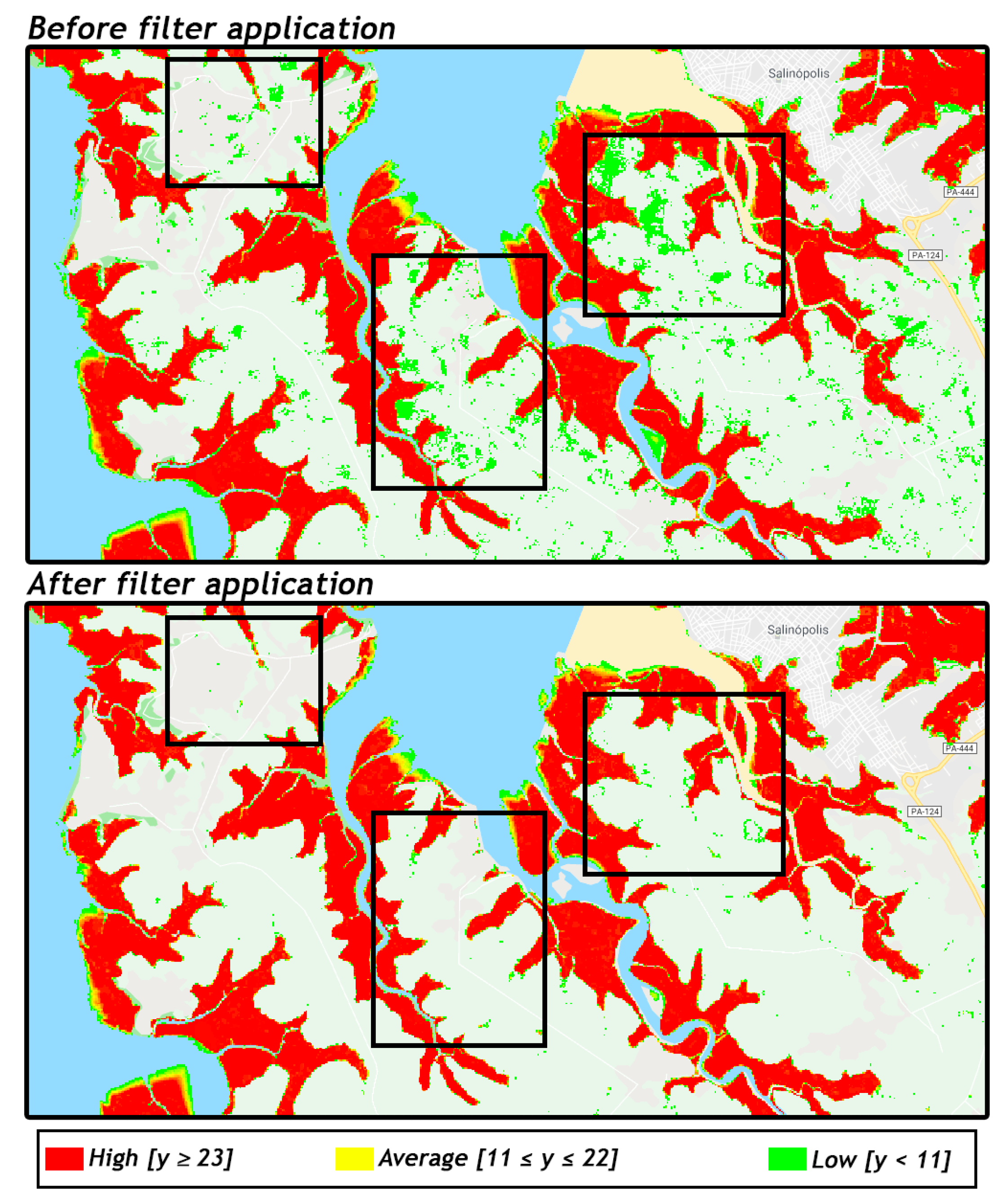
The last step of the filter chain is the frequency filter, as shown in Figure 5. This filter takes into consideration the mangrove occurrence frequency throughout the entire time series. Thus, all mangrove occurrences with less than 10% temporal persistence (3 years or fewer out of 33) are filtered out and incorporated into the non-mangrove class. This mechanism contributes to reducing the temporal oscillation of the mangrove signal, decreasing the number of false positives and preserving consolidated mangrove pixels.
Finally, contingency table analyses [51,52] were used to compare two distinct products: (1) the MMRI spectral separability and (2) the Brazilian mangrove/non-mangrove map. The contingency table cross-tabulates the Mg and N-Mg classes of the reference map and the classified products; thus, a map-to-map analysis was performed. From the contingency table, the following metrics were calculated: the overall agreement (OA); the mangrove positive disagreement proportion (MgPDp), which refers to the proportion of mangrove pixels that are exclusive to the classified maps; and the mangrove negative disagreement proportion (MgNDp), which is the proportion of mangrove pixels exclusive to the reference map.
To examine the performance of the MMRI mangrove separability, a comparison of distinct mangrove and classical vegetation indices was performed. Each map was constructed based on a single-attribute classifier, in which only one of the following spectral indices per execution were considered: Combined Mangrove Recognition Index (CMRI) [38,53], NDVI [33], NDWI [34] or MMRI. The CMRI [53] and the NDWI-NDVI difference [38] are technically the same, as both are simple arithmetical differences between the NDVI and the NDWI, in which the order of the variables changes from “” to “”. This rearrangement imposes a histogram brightness reversal but does not amplify the separability between the mangrove and non-mangrove strata. Thus, for the sake of simplicity, only the NDVI [33], the NDWI [34], the CMRI [53] and the MMRI were further compared.
Each classification was trained based on the same set of samples, with a total of one thousand (1000) training samples collected, five hundred (500) per class. The training sample distribution obeyed a stratified strategy, where the mangrove/non-mangrove data obtained from the Socioeconomic Data and Applications Center (SEDAC) [54] served as stratifying reference. To assess the performance of each index in distinguishing between mangrove and non-mangrove pixels and defining how distinct are the mangrove/non-mangrove strata, a contingency table analysis was performed and the kappa coefficient (KC) and the Bhattacharya coefficient (BC) were computed.
The testing dataset used to evaluate the performance of each index was independent of the training dataset. The testing dataset was designed based on a new round of stratified random sampling over the same reference [54]. This analysis took place along the Caucaia mangrove patch in the metropolitan region of Fortaleza in the Northeast Region of Brazil.
The agreement level of the national-scale maps was derived from three distinct dataset sources: the SEDAC [54] dataset, serving as a reference for the year 2000 mapping; the Global Mangrove Watch (GMW) Project [16], providing the 2010 reference data; and the Chico Mendes Institute for Biodiversity Conservation (ICMBio)—Brazilian Atlas of Mangroves [29], which was used to evaluate the 2013 mapping agreement. As before, all samples used to assess the national agreement measures were entirely independent of the training dataset. A total of twenty thousand (20,000) samples per year were used, with ten thousand (10,000) samples in each class. Finally, all the results, from the auxiliary products to the final annual maps, were made publicly available in raster and vector formats on a Web platform: www.solved.eco.br/mangroveplatform.
3. Results
3.1. Modular Mangrove Recognition Index (MMRI)
Spectral indices may be described as the mathematical combinations of bands used to indicate the relative abundance of features of interest or to enhance the spectral separability between them. With this in mind, the MMRIs were compared to already existing mangrove indices and classical vegetation indices, such as the CMRI [53], the NDVI [33] and the NDWI [34].
Based on a set of modular operations and to present a normalized difference structure (normalized ratio), the MMRI imposes an enhancement of the mangrove/non-mangrove contrast level while simultaneously redefining the resultant mathematical limits to fit the usual −1 to 1 interval. Figure 6 shows the visual aspect of each index, as well as a contingency table from which the overall agreement, the mangrove positive disagreement proportion, the mangrove negative disagreement proportion and the kappa coefficient were calculated, as well as the Bhattacharya coefficient, which denotes the spectral distance between mangrove and non-mangrove pixels.
Regardless of the aspect to be considered—whether visual characteristics, contingency table attributes or the spectral distinction between mangrove and non-mangrove classes—the classification based exclusively on the MMRI achieved more robust results than did those based solely on NDVI, NDWI or the difference between these two. All the metrics, the overall agreement, the mangrove positive disagreement proportion, the mangrove negative disagreement proportion and the kappa coefficient were better or equivalent in the MMRI classification (Figure 6).
Regarding the agreement metrics, the OA and the KC, the values reported by the MMRI mapping were ~1.5 and ~4 times higher, respectively, than the values reported by the remaining indices. Likewise, the disagreement metrics were ~4 times lower in the MMRI results, which indicates a more significant agreement between the MMRI classification and the reference used.
From the perspective of mangrove and non-mangrove spectral separability, the Bhattacharya coefficient applied to the MMRI reached the value of 0.22, which is the lowest among all the calculated coefficients (Figure 6). This suggests that the referred index provides greater distinction between the mangrove and non-mangrove strata compared to the other evaluated indices. The BC is a spectral distance metric that measures the overlap between two populations or samples, where a value of zero represents no overlap and a value of one represents perfect overlap [55].
3.2. Brazilian Mangrove Status
For the first time in the scientific literature, Brazilian mangrove cover mapping was systematically and continuously carried out, producing maps and annual statistics ranging from 1985 to 2018, as shown in Figure 7. Data of this nature allow a better understanding of the dynamics of Brazilian mangroves, updating the status of this type of coverage throughout the country over a span of 33 years.
In Brazil, mangroves occupied areas of ~9700 km2 in 1985 and ~9900 km2 in 2018, representing an area increase of ~200 km2. It is imperative, however, not to rush the interpretation that Brazilian mangroves have experienced a regeneration movement over the past three decades. The percentage difference between 1985 and 2018 is ~2%.
Compared to previous mappings [16,29,54], which refer to the years 2000, 2010 and 2013, respectively, the areas reported here are 4% more, 7% more and 28% less, respectively. In absolute terms, the difference for the year 2000 was ~400 km2, with the value reported by the reference reaching ~9600 km2 and the value calculated here was ~10,010 km2. For the year 2010, the difference was 800 km2, with the reference indicating 10,900 km2, and this manuscript yielding 10,100 km2. Finally, for 2013, the values differed by ~3900 km2, with 13,989 km2 according to the reference and ~10,020 km2 calculated by us.
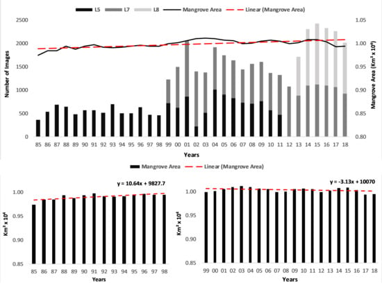
The overall pattern shows an upward trend (Figure 7 and Figure 8). However, from 1985 to March 1998, only the Landsat-5 satellite remained operational. In this period, for the BCZ, the average number of images per year was ~500. In the last decade between 2008 and 2018, this figure tripled to ~1500 images per year, as shown in Figure 8.
On a regional scale, the states of Maranhão, Pará, Amapá and Bahia are the federal units with the most extensive mangrove cover in the country, reaching ~4350 km2 (~46% of the national coverage), ~2100 km2 (~22%), ~830 km2 (~9%) and ~ 670 km2 (~7%), respectively, in 2018. Together, the four states represent ~85% of Brazil’s mangrove cover, as shown in Figure 9.
From the perspective of mangrove cover persistence, ~75% of the Brazilian mangroves remained unchanged for two decades or more, ~10% remained stable between one and two decades and ~15% remained stable for ten or fewer years. In this scenario, the state of Amapá is the state that shows the lowest stability, at ~40%, followed by the states of the south-eastern and southern regions of the country, Espírito Santo, Rio de Janeiro, São Paulo and Santa Catarina, which all present levels of stability between 60% and 65%, as shown in Figure 10.
Since the 1980s, mangrove cover mapping at diverse scales has been carried out, although in a non-systematic way. Here, three sets of data—two global datasets [16,54] from 2000 and 2010, respectively, and one national dataset [29] from 2013—were used to test the concordance levels between the mapping presented in this article and the references cited above. Figure 11 below shows the contingency tables for the years 2000, 2010 and 2013.
Compared to the year 2000 reference data [54], the mapping developed herein achieves an overall agreement of 87% (OA = 0.87) and a kappa coefficient of 74% (KC = 0.74), and presents a low proportion of mangrove negative disagreement, MgNDp = 2% (0.02). There are, however, a large number of positive disagreements, namely, 2474 pixels or ~25% (0.25).
In relation to the 2010 reference [16], the mapping developed herein also achieves a great level of overall agreement, with OA = 85% (0.85) followed by a kappa coefficient of 70%, KC = 0.70. The MgNDp reached ~1% (0.01). On the other hand, the proportion of positive disagreements was ~29% (0.29).
For the year 2013, based on the data produced by the Chico Mendes Institute for Biodiversity Conservation (ICMBio) [29], the smallest kappa coefficient and overall agreement were achieved, KC = 60% (0.60) and OA = 80% (0.80), and the highest negative disagreement proportion was reached, MgNDp = 40% (0.40). The proportion of positive disagreement was low, MgPDp = 1% (0.01).
3.3. Filter-Chain Influence
In total, four different filters may have influenced a resultant classification: gap-fill, temporal, spatial and frequency filters. The first one, gap-fill, may only add mangrove data into a given year; it is an exclusively positive filter (PF). The last two, the spatial and frequency filters, will only remove mangrove pixels from a given year and are therefore negative filters (NF). The temporal filter is the only filter that may add or remove mangrove classifications, depending on the pixel temporal trajectory. Below, Figure 12 and Table 3 categorized and aggregated each pixel, year by year, according to its filtered or no-change aspect, which varied as follows: positive filter (mangrove addition), negative filter (mangrove removal) or unmodified (no change).
The mean percentage values for positive and negative filters were relatively low: 17% and 18%, respectively. On the other hand, the annual average values for the no-change pixels were quite high: 82%. The highest quantity of positive filtering happened in 1995, whereas the lowest appeared in 2006. The highest (24%) and lowest (9%) values of negative filtering appeared in 2017 and 1995, respectively. From 2000 until 2018, the NC percentages were always above the average.
4. Discussion
For the first time in the scientific literature, Brazilian mangrove cover has been systematically and exhaustively mapped. Although data of this nature allow a better understanding of the dynamics of mangrove coverage, it is necessary to understand the effects of the non-homogeneous distribution of Landsat data throughout the time series to avoid superficial interpretations regarding the recorded fluctuations in the country’s mangrove areas.
In scenarios of low data frequency, such as the period from 1985 to 1998, it is reasonable to observe a degradation of the quality of “cloud-free composites” since these are based on the median behaviour of pixels composing the orbital data stack. Therefore, the smaller the number of pixels for a given position of the matrix, the higher the likelihood of including atmospheric and radiometric noise as part of the composite, and thus, the decision of the classifier is less accurate in distinguishing between the categories of mangrove and non-mangrove.
When compared separately, the periods from 1985 to 1998 and 1999 to 2018 show distinct trends, as shown in Figure 8 and Figure 9. The first period, from 1985 to 1998, shows an upward trend with a positive slope, as shown by the equation y = 10.64x + 9827.7. Aside from environmental and human-related changes that are present in this period, most of this pattern of growth seems to be related more to the uneven distribution of Landsat data throughout the 33 years than to a regeneration movement of Brazilian mangroves. From 1989 to 1998, the PF% values were greater than 20%; for five of those years, the PF% values were greater than 40%.
The second period, from 1999 to 2018, when the PF% values are primarily smaller than 10% and the NC% values are above 85%, a slightly negative slope is shown, presenting a trend of mangrove area loss, which is evidenced by the equation y = −3.13x + 10070 and compatible with the global standard expected for mangrove coverage in recent decades [56].
In absolute terms, the direct difference between the years 2000 and 2018 shows an area loss of approximately 70 km2: a difference of ~0.6%. However, it is interesting to note that there is a wave-like pattern present in the variation in mangrove areas. Upon comparing the data from 2003, which has the largest reported area of mangroves, and the 2017 data, which has the smallest quantified area, the absolute difference is ~200 km2, which represents an area loss of ~2%, a value almost three times greater than that previously reported by the comparison between 2000 and 2018.
This pattern may be associated with intra-annual oceanographic and climatic variables (rainy and dry seasons), which alter the prevailing tide and humidity conditions in the median composites [57,58,59,60]. On one-year intervals, especially over areas often covered by clouds such as the BCZ, the definition of additional image-selection parameters (e.g., the tide condition and the dominant climatic pattern) greatly reduces the number of images available, which makes spatial analysis over shorter time frames impractical.
Regarding the concordance levels, when compared to the year 2000 data [54], an overall agreement of 87% and a kappa coefficient of 74%, KC = 0.74, were reached. However, for this reference, there is a large quantity of positive disagreements, which is reflected by the MgPDp of ~25%. Nevertheless, most of these positive differences may be associated with unfiltered clouds and shadow residues in the reference, which were included as part of the non-mangrove class and thus generated positive disagreement.
In comparison to the 2010 data [16], there is significant overall agreement between the published data and our mapping effort, reaching an overall agreement of 85% and a kappa coefficient of 70%. However, the MgNDp is approximately 29%, which is likely to be associated with differences between the edges of the mangrove classes (border errors) and to the inclusion of the coastal rivers’ dendritic patterns as part of the mangrove reference class.
For 2013, the year with the greatest mangrove area difference between the reference and our map, approximately 28% (~3900 km2), and the lowest overall agreement and kappa coefficient, 80% and 60%, respectively, the mangrove concept adopted by the reference was different. Unlike the previous concepts, [29] focused on ecosystem identification rather than mangrove forests [16,54]. Thus, the omissions are quite high and the MgNDp reaches nearly 40%. Furthermore, the reference was created through visual interpretation and, therefore, had a reduced need for the application of spatial filters. As a result, the reported omissions are minorly associated with border differences and are mostly attributed to the inclusion of “apicuns” (salt marshes) as part of the mangrove reference class.
Moreover, it is necessary to highlight the difficulties of implementing continental-scale mapping in a systematic and exhaustive way. The uneven distribution of Landsat data, scarce prior to 1998 and much more frequent in the last two decades, imposes obstacles within the construction of annual cloud-free composites because the quantity of orbital data is greatly unbalanced over time.
Increasing the composites’ temporal windows to three or more years may be important to sharply select data that match specific climatic and oceanographic conditions. In addition, the use of multiple satellite families (Landsat and Sentinel, for example) should also be considered as an alternative to increase the frequency of observations.
Compared to previous mappings produced on an approximately annual timeframe, without considering the prevailing tide and climatic conditions and focusing on mangrove vegetation mapping, the results expressed herein are spatially coherent, reaching a kappa coefficient of 0.7 and an overall agreement above 0.85, as seen in Figure 11.
Along with a broader temporal window, the restriction of the climatic pattern (rainy or dry), as well as the selection of data in specific tide conditions, whether high or low, can reduce the wave-like pattern associated with the reported mangrove areas. Furthermore, the addition of more detailed land use/land cover classes seems to be essential to the ability to identify and separate natural coastal changes from anthropogenic coastal changes, as a more detailed pixel trajectory would allow a more accurate identification of human interference.
From the standpoint of MMRI robustness, compared to other indices, the MMRI seems to provide a greater distinction between the mangrove and non-mangrove strata, which facilitates the discrimination of such classes by automatic classifiers. The new index can be used in conjunction with multiple families of satellites, digital elevation models (DEM) and microwave data and, whenever possible, can incorporate information from the main domains and subdomains of remote sensing, space, time, spectra and context.
The next steps of this research include the creation of a mechanism capable of identifying tidal conditions from orbital data, the expansion of the analysis to the South American continent, and the insertion of new classes of coastal environments such as “apicuns”, beaches and dunes, aquaculture and urban areas, which would help separate human-related changes from natural coastal changes.
5. Conclusions
This manuscript detailed a GEE-managed pipeline to discriminate mangrove forests from surrounding vegetation. The developed pipeline is scalable and suitable for large-scale mangrove cover analyses, allowing systematic and continuous mapping of the Brazilian mangrove cover and producing maps and annual statistics ranging from 1985 to 2018. When compared to previous research at global and national scales, the data produced have high levels of spatial and statistical agreement. All the data produced are available for download through the website http://www.solved.eco.br/mangroveplatform and will be transferred to the MapBiomas project (www.mapbiomas.org) in MapBiomas Collection 4.0.
The developed spectral index, MMRI, was demonstrated to be robust and helped to increase the spectral separability between the mangrove and non-mangrove classes. The expansion of the temporal window for the construction of mosaics, the restriction of the climatic pattern (rainy or dry) and the ability to discern between the predominant tidal regimes, whether high or low, may help reduce the area fluctuations associated with the coverage of mangroves.
Author Contributions
Conceptualization, C.D. and L.C.; methodology, C.D. and L.C.; software, L.C., G.N. and J.R.; validation, C.D., L.S. and M.A.; formal analysis, C.D.; investigation, C.D.; resources, P.W.M.S.-F.; data curation, C.D., M.A. and P.W.M.S-F.; writing—original draft preparation, C.D.; writing—review and editing, C.D., M.A. and P.W.M.S-F.; visualization, C.D and L.S.; supervision, P.W.M.S-F.; project administration, P.W.M.S-F.; funding acquisition, P.W.M.S-F.
Funding
This research was funded by the Brazilian National Council for Scientific and Technological Development (CNPq): 870005/1997-9 and the MapBiomas Project. The processing charges were covered by the Dean of Research and Graduate Studies (PROPESP) from the Federal University of Para (UFPA).
Acknowledgments
The authors are grateful to Tasso Azevedo, general coordinator of the MapBiomas Project and the System for Estimation of Green House Gases Emissions (SEEG) initiative, Carlos Souza Jr., senior researcher at the Amazon Institute (IMAZON) and Washington Rocha, full professor at Feira de Santana State University (UEFS), for their useful comments, suggestions and encouragement. The authors would like to thank the anonymous reviewers and the editor for their helpful and constructive comments that greatly contributed to improving this paper. Lastly, the authors acknowledge the Norwegian Government for the financial support given to the Mapbiomas Project, via World Resources Institute (WRI), and Google for the development of the Google Earth Engine platform.
Conflicts of Interest
The authors declare no conflict of interest.
References
- Neumann, B.; Vafeidis, A.T.; Zimmermann, J.; Nicholls, R.J. Future Coastal Population Growth and Exposure to Sea-Level Rise and Coastal Flooding—A Global Assessment. PLoS ONE 2015, 10, e0118571. [Google Scholar] [CrossRef]
- Small, C.; Nicholls, R.J. A Global Analysis of Human Settlement in Coastal Zones. J. Coast. Res. 2003, 19, 584–599. [Google Scholar] [CrossRef]
- Burke, L.; Kura, Y.; Kassem, K.; Revenga, C.; Spalding, M.; McAllister, D. Pilot Analysis of Global Ecosystems: Coastal Ecosystems; World Recourses Institute: Washington, DC, USA, 2001. [Google Scholar]
- Nicolodi, J.L.; Petermann, R.M. Potential vulnerability of the Brazilian coastal zone in its environmental, social, and technological aspects. Panam. J. Aquat. Sci. 2010. [Google Scholar] [CrossRef]
- Dominguez, J.M.L. The Coastal Zone of Brazil. In Geology and Geomorphology of Holocene Coastal Barriers of Brazil; Springer: Berlin/Heidelberg, Germany, 2009; pp. 17–51. ISBN 978-3-540-44771-9. [Google Scholar]
- Giri, C. Observation and Monitoring of Mangrove Forests Using Remote Sensing: Opportunities and Challenges. Remote Sens. 2016, 8, 783. [Google Scholar] [CrossRef]
- Giri, C.; Ochieng, E.; Tieszen, L.L.; Zhu, Z.; Singh, A.; Loveland, T.; Masek, J.; Duke, N. Status and distribution of mangrove forests of the world using earth observation satellite data. Glob. Ecol. Biogeogr. 2011, 20, 154–159. [Google Scholar] [CrossRef]
- Alongi, D.M. The Energetics of Mangrove Forests, 1st ed.; Springer: Dordrecht, The Netherlands, 2009; ISBN 978-1-4020-4270-6. [Google Scholar]
- Alongi, D.M. Mangrove forests: Resilience, protection from tsunamis, and responses to global climate change. Estuar. Coast. Shelf Sci. 2008, 76, 1–13. [Google Scholar] [CrossRef]
- Murdiyarso, D.; Purbopuspito, J.; Kauffman, J.B.; Warren, M.W.; Sasmito, S.D.; Donato, D.C.; Manuri, S.; Krisnawati, H.; Taberima, S.; Kurnianto, S. The potential of Indonesian mangrove forests for global climate change mitigation. Nat. Clim. Chang. 2015, 5, 1089–1092. [Google Scholar] [CrossRef]
- Saenger, P.; Hegerl, E.J.; Davie, J.D.S. Global Status of Mangrove Ecosystems; International Union for Conservation of Nature and Natural Resources: Gland, Switzerland, 1983. [Google Scholar]
- Alongi, D.M. Present state and future of the world’s mangrove forests. Environ. Conserv. 2002, 29, 331–349. [Google Scholar] [CrossRef]
- Donato, D.C.; Kauffman, J.B.; Murdiyarso, D.; Kurnianto, S.; Stidham, M.; Kanninen, M. Mangroves among the most carbon-rich forests in the tropics. Nat. Geosci. 2011, 4, 293–297. [Google Scholar] [CrossRef]
- Spalding, M.; Kainuma, M.; Collins, L. World Atlas of Mangroves; Taylor & Francis Group: Abingdon-on-Thames, UK, 2010; ISBN 9781849776608. [Google Scholar]
- Thomas, N.; Bunting, P.; Lucas, R.; Hardy, A.; Rosenqvist, A.; Fatoyinbo, T. Mapping Mangrove Extent and Change: A Globally Applicable Approach. Remote Sens. 2018, 10, 1466. [Google Scholar] [CrossRef]
- Bunting, P.; Rosenqvist, A.; Lucas, M.R.; Rebelo, L.-M.; Hilarides, L.; Thomas, N.; Hardy, A.; Itoh, T.; Shimada, M.; Finlayson, M.C. The Global Mangrove Watch—A New 2010 Global Baseline of Mangrove Extent. Remote Sens. 2018, 10, 1669. [Google Scholar] [CrossRef]
- Herz, R. Manguezais do Brasil; United States Pharmacopeia (USP): North Bethesda, MD, USA, 1991. [Google Scholar]
- Schaeffer-Novelli, Y.; Cintrón-Molero, G.; Adaime, R.R.; de Camargo, T.M.; Cintron-Molero, G.; de Camargo, T.M. Variability of Mangrove Ecosystems along the Brazilian Coast. Estuaries 1990, 13, 204–218. [Google Scholar] [CrossRef]
- Souza Filho, P.W.M. Costa de manguezais de macromaré da Amazônia: Cenários morfológicos, mapeamento e quantificação de áreas usando dados de sensores remotos. Rev. Bras. Geofísica 2005, 23, 427–435. [Google Scholar] [CrossRef]
- Walfir Martins Souza Filho, P.; Renato Paradella, W. Recognition of the main geobotanical features along the Bragança mangrove coast (Brazilian Amazon Region) from Landsat TM and RADARSAT-1 data. Wetl. Ecol. Manag. 2002, 10, 121–130. [Google Scholar] [CrossRef]
- Souza Filho, P.W.M.; Paradella, W.R. Use of RADARSAT-1 fine mode and Landsat-5 TM selective principal component analysis for geomorphological mapping in a macrotidal mangrove coast in the Amazon Region. Can. J. Remote Sens. 2005, 31, 214–224. [Google Scholar] [CrossRef]
- Rodrigues, S.W.P.; Souza-Filho, P.W.M. Use of Multi-Sensor Data to Identify and Map Tropical Coastal Wetlands in the Amazon of Northern Brazil. Wetlands 2011, 31, 11–23. [Google Scholar] [CrossRef]
- Nascimento Jr, W.R.; Souza-Filho, P.W.M.; Proisy, C.; Lucas, R.M.; Rosenqvist, A. Mapping changes in the largest continuous Amazonian mangrove belt using object-based classification of multisensor satellite imagery. Estuar. Coast. Shelf Sci. 2013, 117, 83–93. [Google Scholar] [CrossRef]
- Santos, L.C.M.; Matos, H.R.; Schaeffer-Novelli, Y.; Cunha-Lignon, M.; Bitencourt, M.D.; Koedam, N.; Dahdouh-Guebas, F. Anthropogenic activities on mangrove areas (São Francisco River Estuary, Brazil Northeast): A GIS-based analysis of CBERS and SPOT images to aid in local management. Ocean Coast. Manag. 2014, 89, 39–50. [Google Scholar] [CrossRef]
- Queiroz, L.; Rossi, S.; Meireles, J.; Coelho, C. Shrimp aquaculture in the federal state of Ceará, 1970–2012: Trends after mangrove forest privatization in Brazil. Ocean Coast. Manag. 2013, 73, 54–62. [Google Scholar] [CrossRef]
- Rocha de Souza Pereira, F.; Kampel, M.; Cunha-Lignon, M. Mapping of mangrove forests on the southern coast of São Paulo, Brazil, using synthetic aperture radar data from ALOS/PALSAR. Remote Sens. Lett. 2012, 3, 567–576. [Google Scholar] [CrossRef]
- Pereira, F.; Kampel, M.; Cunha-Lignon, M. Mangrove vegetation structure in Southeast Brazil from phased array L-band synthetic aperture radar data. J. Appl. Remote Sens. 2016, 10, 036021. [Google Scholar] [CrossRef] [Green Version]
- Magris, R.A.; Barreto, R. Mapping and assessment of protection of mangrove habitats in Brazil. Panam. J. Aquat. Sci. 2010, 5, 546–556. [Google Scholar]
- ICMBio. Atlas dos Manguezais do Brasil, 1st ed.; ICMBio: Brasilia, Brazil, 2017; ISBN 978-85-61842-75-8. [Google Scholar]
- Gorelick, N.; Hancher, M.; Dixon, M.; Ilyushchenko, S.; Thau, D.; Moore, R. Google Earth Engine: Planetary-scale geospatial analysis for everyone. Remote Sens. Environ. 2017, 202, 18–27. [Google Scholar] [CrossRef]
- Chen, X.; Huang, X.; Jiao, C.; Flanner, M.G.; Raeker, T.; Palen, B. Running climate model on a commercial cloud computing environment: A case study using Community Earth System Model (CESM) on Amazon AWS. Comput. Geosci. 2017, 98, 21–25. [Google Scholar] [CrossRef]
- Zhu, Z.; Wang, S.; Woodcock, C.E. Improvement and expansion of the Fmask algorithm: Cloud, cloud shadow, and snow detection for Landsats 4–7, 8, and Sentinel 2 images. Remote Sens. Environ. 2015, 159, 269–277. [Google Scholar] [CrossRef]
- Tucker, C.J. Red and photographic infrared linear combinations for monitoring vegetation. Remote Sens. Environ. 1979, 8, 127–150. [Google Scholar] [CrossRef] [Green Version]
- McFeeters, S.K. The use of the Normalized Difference Water Index (NDWI) in the delineation of open water features. Int. J. Remote Sens. 1996, 17, 1425–1432. [Google Scholar] [CrossRef]
- Gao, B. NDWI—A normalized difference water index for remote sensing of vegetation liquid water from space. Remote Sens. Environ. 1996, 58, 257–266. [Google Scholar] [CrossRef]
- Tong, P.H.S.; Auda, Y.; Populus, J.; Aizpuru, M.; Al Habshi, A.; Blasco, F. Assessment from space of mangroves evolution in the Mekong Delta, in relation to extensive shrimp farming. Int. J. Remote Sens. 2004, 25, 4795–4812. [Google Scholar] [CrossRef]
- Fei, S.X.; Shan, C.H.; Hua, G.Z. Remote Sensing of Mangrove Wetlands Identification. Procedia Environ. Sci. 2011, 10, 2287–2293. [Google Scholar] [CrossRef] [Green Version]
- Alsaaideh, B.; Al-Hanbali, A.; Tateishi, R.; Kobayashi, T.; Hoan, N.T. Mangrove Forests Mapping in the Southern Part of Japan Using Landsat ETM+ with DEM. J. Geogr. Inf. Syst. 2013, 5, 9. [Google Scholar] [CrossRef]
- Nardin, W.; Locatelli, S.; Pasquarella, V.; Rulli, M.C.; Woodcock, C.E.; Fagherazzi, S. Dynamics of a fringe mangrove forest detected by Landsat images in the Mekong River Delta, Vietnam. Earth Surf. Process. Landforms 2016, 41, 2024–2037. [Google Scholar] [CrossRef]
- Pham, D.T.; Yokoya, N.; Bui, T.D.; Yoshino, K.; Friess, A.D. Remote Sensing Approaches for Monitoring Mangrove Species, Structure, and Biomass: Opportunities and Challenges. Remote Sens. 2019, 11, 230. [Google Scholar] [CrossRef]
- Kuenzer, C.; Bluemel, A.; Gebhardt, S.; Quoc, T.V.; Dech, S. Remote Sensing of Mangrove Ecosystems: A Review. Remote Sens. 2011, 3, 878–928. [Google Scholar] [CrossRef] [Green Version]
- USGS Landsat. 8 (L8)Data Users Handbook; USGS Landsat: Sioux Falls, SD, USA, 2015.
- Storey, J.; Choate, M.; Lee, K. Landsat 8 Operational Land Imager On-Orbit Geometric Calibration and Performance. Remote Sens. 2014, 6, 11127–11152. [Google Scholar] [CrossRef] [Green Version]
- Teillet, P.M.; Barker, J.L.; Markham, B.L.; Irish, R.R.; Fedosejevs, G.; Storey, J.C. Radiometric cross-calibration of the Landsat-7 ETM+ and Landsat-5 TM sensors based on tandem data sets. Remote Sens. Environ. 2001, 78, 39–54. [Google Scholar] [CrossRef] [Green Version]
- USGS Landsat. USGS Landsat Collection 1 Level 1 Product Definition; USGS Landsat: Sioux Falls, SD, USA, 2017; Volume 26.
- Liu, H.Q.; Huete, A. Feedback based modification of the NDVI to minimize canopy background and atmospheric noise. IEEE Trans. Geosci. Remote Sens. 1995, 33, 457–465. [Google Scholar] [CrossRef]
- Xu, H. Modification of normalised difference water index (NDWI) to enhance open water features in remotely sensed imagery. Int. J. Remote Sens. 2006, 27, 3025–3033. [Google Scholar] [CrossRef]
- Rogers, A.S.; Kearney, M.S. Reducing signature variability in unmixing coastal marsh Thematic Mapper scenes using spectral indices. Int. J. Remote Sens. 2004. [Google Scholar] [CrossRef]
- Gu, Y.; Brown, J.F.; Verdin, J.P.; Wardlow, B. A five-year analysis of MODIS NDVI and NDWI for grassland drought assessment over the central Great Plains of the United States. Geophys. Res. Lett. 2007, 34. [Google Scholar] [CrossRef] [Green Version]
- Bogner, C.; Seo, B.; Rohner, D.; Reineking, B. Classification of rare land cover types: Distinguishing annual and perennial crops in an agricultural catchment in South Korea. PLoS ONE 2018, 13, e0190476. [Google Scholar] [CrossRef] [PubMed]
- Olofsson, P.; Foody, G.M.; Herold, M.; Stehman, S.V.; Woodcock, C.E.; Wulder, M.A. Good practices for estimating area and assessing accuracy of land change. Remote Sens. Environ. 2014, 148, 42–57. [Google Scholar] [CrossRef] [Green Version]
- Pontius, R.G.; Santacruz, A. Quantity, exchange, and shift components of difference in a square contingency table. Int. J. Remote Sens. 2014, 35, 7543–7554. [Google Scholar] [CrossRef]
- Gupta, K.; Mukhopadhyay, A.; Giri, S.; Chanda, A.; Datta Majumdar, S.; Samanta, S.; Mitra, D.; Samal, R.N.; Pattnaik, A.K.; Hazra, S. An index for discrimination of mangroves from non-mangroves using LANDSAT 8 OLI imagery. MethodsX 2018, 5, 1129–1139. [Google Scholar] [CrossRef] [PubMed]
- Giri, C.; Ochieng, E.; Tieszen, L.L.; Zhu, Z.; Singh, A.; Loveland, T.; Masek, J.; Duke, N. Global Mangrove Forests Distribution, 2000; NASA Socioeconomic Data and Applications Center (SEDAC): Palisades, NY, USA, 2013. [Google Scholar]
- Ben Ayed, I.; Punithakumar, K.; Li, S. Distribution Matching with the Bhattacharyya Similarity: A Bound Optimization Framework. IEEE Trans. Pattern Anal. Mach. Intell. 2015, 37, 1777–1791. [Google Scholar] [CrossRef] [PubMed]
- Thomas, N.; Lucas, R.; Bunting, P.; Hardy, A.; Rosenqvist, A.; Simard, M. Distribution and drivers of global mangrove forest change, 1996–2010. PLoS ONE 2017, 12, e0179302. [Google Scholar] [CrossRef]
- Xia, Q.; Qin, C.-Z.; Li, H.; Huang, C.; Su, F.-Z. Mapping Mangrove Forests Based on Multi-Tidal High-Resolution Satellite Imagery. Remote Sens. 2018, 10, 1343. [Google Scholar] [CrossRef]
- Rogers, K.; Lymburner, L.; Salum, R.; Brooke, B.P.; Woodroffe, C.D. Mapping of mangrove extent and zonation using high and low tide composites of Landsat data. Hydrobiologia 2017, 803, 49–68. [Google Scholar] [CrossRef]
- Zhang, X.; Treitz, P.M.; Chen, D.; Quan, C.; Shi, L.; Li, X. Mapping mangrove forests using multi-tidal remotely-sensed data and a decision-tree-based procedure. Int. J. Appl. Earth Obs. Geoinf. 2017, 62, 201–214. [Google Scholar] [CrossRef]
- Chen, B.; Xiao, X.; Li, X.; Pan, L.; Doughty, R.; Ma, J.; Dong, J.; Qin, Y.; Zhao, B.; Zhixiang, W.; et al. A mangrove forest map of China in 2015: Analysis of time series Landsat 7/8 and Sentinel-1A imagery in Google Earth Engine cloud computing platform. ISPRS J. Photogramm. Remote Sens. 2017, 131, 104–120. [Google Scholar] [CrossRef]
Figure 1.
Data-flow diagram. All processing and analysis occur inside the Google Earth Engine (GEE) platform. Steps related to image processing are in blue. The steps in green are related to the sample design. Classification procedures are in yellow. The concordance assessment phase is in red and, finally, the data availability is in salmon. BQA and SRTM denotes Band Quality Assessment and Shuttle Radar Topography Mission, respectively.

Figure 2.
The Brazilian coastal region was split into six (6) distinct sectors. Site 1—Amapá; Site 2—Marajó Island; Site 3—Pará/Maranhão; Site 4—Piauí/Bahia; Site 5—Espírito Santo/São Paulo; and Site 6—Paraná/Laguna (SC). The north and south boundaries of the Brazilian mangroves are in green. The black grids represent the WRS-2 Path and Row footprints. The following acronyms represent the Brazilian coastal states: AL (Alagoas), AP (Amapá), BA (Bahia), CE (Ceará), ES (Espírito Santo), MA (Maranhão), PA (Pará), PB (Paraíba), PE (Pernambuco), PI (Piauí), PR (Paraná), RJ (Rio de Janeiro), RN (Rio Grande do Norte), SC (Santa Catarina), SE (Sergipe) and SP (São Paulo).

Figure 3.
Gap-filling mechanism. The next valid classification replaces existing no-data values. If no “future” valid position is available, then the no-data value is replaced by its previous valid classification, based on up to a maximum of three (3) prior years. To keep track of pixel temporal origins, a mask of years was built.

Figure 4.
The spatial filter removes pixels that do not share neighbours of identical value. The minimum connection value was 10 pixels.
Figure 4.
The spatial filter removes pixels that do not share neighbours of identical value. The minimum connection value was 10 pixels.

Figure 5.
Red, yellow and green represent mangrove pixels with high (23 or more years, y ≥ 23), average (between 11 and 22 years, 11 ≤ y ≤ 22) and low (ten years or less, y < 11) occurrence frequencies, respectively. The top image shows mangrove pixels before applying the frequency filter. The bottom image shows mangrove pixels after applying the frequency filter. The black boxes are centred on areas that have been significantly affected by the filter. Note that all mangrove occurrences with less than 10% temporal persistence (3 years in 33 possible years) were filtered out.

Figure 6.
The first row shows the visual aspects of each index—NDVI, NDWI, CMRI and MMRI. The second row shows the classification results. The bottom row shows the contingency tables, where Mg stands for the mangrove class and N-Mg stands for the non-mangrove class. OA stands for overall agreement, MgPDp indicates mangrove positive disagreement proportion, MgNDp refers to mangrove negative disagreement proportion, KC means the kappa coefficient and BC denotes the Bhattacharya coefficient.

Figure 7.
Brazilian mangrove areas from 1985 to 2018. The x-axis represents the years of the study. The y-axis represents total area of Brazilian mangroves in ten thousand kilometers squared. The numbers above each bar are the area values for that bar.
Figure 7.
Brazilian mangrove areas from 1985 to 2018. The x-axis represents the years of the study. The y-axis represents total area of Brazilian mangroves in ten thousand kilometers squared. The numbers above each bar are the area values for that bar.

Figure 8.
The top image shows the general pattern of fluctuation in the mangrove areas from 1985 to 2018. The solid line represents the variation in mangrove area over time. The dotted line shows the general trend. The bars show the distribution of Landsat images along the time series. L5 stands for Landsat-5, L7 refers to Landsat-7 and L8 stands for Landsat-8. The bottom left image shows the mangrove area variation and trend line from 1985 to 1998. The bottom right image shows the mangrove areas and trends from 1999 to 2018.

Figure 9.
Brazilian mangrove area in percentage of total mangrove cover per state. The x-axis represents the coastal states’ two-letter abbreviations, as in Figure 2. The y-axis represents the mangrove area % of the year 2018.
Figure 9.
Brazilian mangrove area in percentage of total mangrove cover per state. The x-axis represents the coastal states’ two-letter abbreviations, as in Figure 2. The y-axis represents the mangrove area % of the year 2018.

Figure 10.
Brazilian mangrove cover persistence at the national and regional scale. The top bar shows the overall mangrove persistence. The bottom graph shows the mangrove persistence per state, abbreviated as in Figure 2. The x-axis represents the state distributions, whereas the y-axis represents the mangrove cover temporal persistence percentages (%). Black represents 20 years or more of stability, dark grey indicates stability between 10 and 20 years and light grey represents stability for less than 10 years.

Figure 11.
On the left are the 2000, 2010 and 2013 median composites. In the central portion, red represents the mangroves of the reference data, blue denotes the classified mangroves and green represents the agreement between blues and reds. The contingency tables (right) show the agreement levels between the reference and classified data. Values on the main diagonal are the numbers of concordant pixels. On the off-diagonal, those above are positive differences and those below are negative differences. OA stands for overall agreement, MgPDp means the mangrove positive disagreement proportion, MgNDp refers to the mangrove negative disagreement proportion and KC denotes the kappa coefficient.

Figure 12.
On the left is the 1988 MMRI median composite: dark green represents mangroves, light green is non-mangroves and blue is water. In the centre is the 1988 Landsat-5 band 543 median composite. On the right, PF denotes a positive filter (mangrove addition), NF stands for a negative filter (mangrove removal) and NC stands for no change.


Table 1.
Classifier attributes and classification parameters. In total, ten (10) distinct attributes were used. NIR, stands for near-infrared; SWIR1 and SWIR2, short-wave infrareds 1 and 2.
Table 1.
Classifier attributes and classification parameters. In total, ten (10) distinct attributes were used. NIR, stands for near-infrared; SWIR1 and SWIR2, short-wave infrareds 1 and 2.
| Parameters | Values |
|---|---|
| Classifier | Random Forest |
| Trees | 100 |
| Samples | ~1000 per class per sector per year |
| Attributes | 10 (Green, Red, NIR, SWIR1, SWIR2, NDVI, EVI, MNDWI, NDSI, MMRI) |
| Classes | 2 (Mangrove and Non-Mangrove) |
Table 2.
The temporal filter inspects the central position of three consecutive years, and in cases of identical extremities, the centre position is reclassified to match its neighbour. T1, T2 and T3 stand for positions one (1), two (2) and three (3), respectively. GR means “generic rule”, while Mg and N-Mg represent mangrove and non-mangrove pixels.
| Rule | Input (Year) | Output | ||||
|---|---|---|---|---|---|---|
| T1 | T2 | T3 | T1 | T2 | T3 | |
| GR | Mg | N-Mg | Mg | Mg | Mg | Mg |
| GR | N-Mg | Mg | N-Mg | N-Mg | N-Mg | N-Mg |
Table 3.
Annual filter-affected area, in percentages. PF% indicates a positive filter (mangrove addition), PN% stands for a negative filter (mangrove removal) and NC% denotes an unfiltered pixel (no-change).
Table 3.
Annual filter-affected area, in percentages. PF% indicates a positive filter (mangrove addition), PN% stands for a negative filter (mangrove removal) and NC% denotes an unfiltered pixel (no-change).
| Year | 1985 | 1986 | 1987 | 1988 | 1989 | 1990 | 1991 | 1992 | 1993 | 1994 | 1995 | 1996 |
| PF% | 21 | 17 | 18 | 17 | 28 | 24 | 38 | 40 | 47 | 47 | 51 | 47 |
| NF% | 23 | 18 | 15 | 14 | 18 | 22 | 13 | 13 | 17 | 14 | 09 | 11 |
| NC% | 79 | 83 | 82 | 83 | 72 | 76 | 62 | 60 | 53 | 53 | 49 | 53 |
| Year | 1997 | 1998 | 1999 | 2000 | 2001 | 2002 | 2003 | 2004 | 2005 | 2006 | 2007 | 2008 |
| PF% | 27 | 26 | 13 | 05 | 04 | 03 | 04 | 04 | 05 | 03 | 05 | 04 |
| NF% | 10 | 20 | 16 | 12 | 17 | 20 | 18 | 18 | 17 | 16 | 17 | 19 |
| NC% | 73 | 74 | 87 | 95 | 96 | 97 | 96 | 96 | 94 | 97 | 95 | 96 |
| Year | 2009 | 2010 | 2011 | 2012 | 2013 | 2014 | 2015 | 2016 | 2017 | 2018 | ||
| PF% | 06 | 04 | 05 | 10 | 09 | 12 | 07 | 07 | 07 | 10 | ||
| NF% | 13 | 18 | 22 | 22 | 22 | 19 | 19 | 23 | 24 | 10 | ||
| NC% | 94 | 96 | 95 | 91 | 91 | 88 | 93 | 93 | 93 | 90 |
© 2019 by the authors. Licensee MDPI, Basel, Switzerland. This article is an open access article distributed under the terms and conditions of the Creative Commons Attribution (CC BY) license (http://creativecommons.org/licenses/by/4.0/).
Share and Cite
MDPI and ACS Style
Diniz, C.; Cortinhas, L.; Nerino, G.; Rodrigues, J.; Sadeck, L.; Adami, M.; Souza-Filho, P.W.M. Brazilian Mangrove Status: Three Decades of Satellite Data Analysis. Remote Sens. 2019, 11, 808. https://doi.org/10.3390/rs11070808
AMA Style
Diniz C, Cortinhas L, Nerino G, Rodrigues J, Sadeck L, Adami M, Souza-Filho PWM. Brazilian Mangrove Status: Three Decades of Satellite Data Analysis. Remote Sensing. 2019; 11(7):808. https://doi.org/10.3390/rs11070808
Chicago/Turabian StyleDiniz, Cesar, Luiz Cortinhas, Gilberto Nerino, Jhonatan Rodrigues, Luís Sadeck, Marcos Adami, and Pedro Walfir M. Souza-Filho. 2019. "Brazilian Mangrove Status: Three Decades of Satellite Data Analysis" Remote Sensing 11, no. 7: 808. https://doi.org/10.3390/rs11070808
Note that from the first issue of 2016, this journal uses article numbers instead of page numbers. See further details here.