Influence of the System MTF on the On-Board Lossless Compression of Hyperspectral Raw Data


1
Institute of Applied Physics “Nello Carrara”, IFAC-CNR, Research Area of Florence, 50019 Sesto Fiorentino (FI), Italy
2
Department of Information Engineering, University of Florence, 50139 Florence, Italy
*
Author to whom correspondence should be addressed.
Remote Sens. 2019, 11(7), 791; https://doi.org/10.3390/rs11070791
Submission received: 8 February 2019
/
Revised: 11 March 2019
/
Accepted: 25 March 2019
/
Published: 2 April 2019
(This article belongs to the Special Issue Real-Time Processing of Remotely-Sensed Imaging Data)
Abstract
:A noticeable topic to be pursued in the field of on-board real-time data processing is the influence of the modulation transfer function (MTF) of the image acquisition system on the lossless compressibility of raw (that is, uncalibrated) hyperspectral data. Actually, notwithstanding the system device is constrained by several design and manufacturing requirements, the impact of the on-board MTF on the performance of data compressors is becoming remarkable. In particular, the aim of reducing both transmission bandwidth/power and mass storage can be efficiently pursued. Such an analysis is expected to be useful especially for systems employed in mini-satellites, whose payload must be compact and light. From this perspective, this paper investigates the performance of a typical imaging system that acquires low/medium-spatial-resolution images, by considering high-resolution reference data, which simulate the real scene to be imaged. To this end, standard Consultative Committee for Space Data Systems (CCSDS) Aviris 2006 data have been chosen, due to their spatial resolution of m, which is adequate to be a reference for simulated data whose spatial resolution is foreseen between and m. MTF requirements are usually provided based on the cut-off value of the amplitude at the Nyquist frequency, which is defined as a half of the sampling frequency. Typically, a cut-off value between and ensures that a sufficient amount of information is delivered from the scene to the acquired image, by avoiding at the same time the degradation due to an excessive aliasing distortion. All the scores are achieved by running the standard lossless compression scheme CCSDS 1.2.3.0-B-1 for multispectral/hyperspectral data, as a function of the cut-off value and different noise acquisition levels. The final results, and related plots, show that this analysis can suggest a suitable choice for the cut-off value, to ensure both a sufficient quality and low bit rates for the transmitted data to the ground station.
1. Introduction
In this paper, the real-time lossless compressibility of the acquired raw data in a satellite scenario is investigated when changes occur in the MTF of the sensor optical system. In fact, compression procedures are necessary to minimize the data amount to be sent at the ground station, and consequently to alleviate the load of the limited bandwidth in the transmission stage [1,2]. In particular, lossless algorithm ensure the recovering of the original data without any distortion, even if compression ratios (CR) of more of are hardly achievable, because of the degradation relating to several impairments, which are caused by the presence of both internal and external noise sources [3], as acquisition noise, striping, registration errors, cosmic ray interactions, and so on. Moreover, an on-board compression scheme works with reduced memory and computational resources, due to the very challenging space environment. To well cope with designers’ needs, an algorithm must be suboptimal with respect to the state-of-art methods, in particular by resorting to integer arithmetics and to a high redundancy, so that the effects of possible transmission errors can be minimized. Such a factor is on behalf of lossless methods, which are more insensitive to the channel noise, because there is no superimposition between transmission errors and those due to the algorithm itself.
These requirements are particularly challenging in the case of mini-satellites, whose environment requires a very low computational complexity and rather compelling payload constraints. In fact, the main advantages of such missions are a significant cost reduction, with a consequent economical effectiveness, as well as an improved compactness, which is achievable thanks to the continuous technological progresses, in such a way that payloads of a few kilograms can produce measurements of the requested precision [4]. In this context, the Italian Space Agency (ASI) supports the PLATiNO program (Mini Piattaforma spaziaLe ad Alta TecNOlogia, that is, Mini Spatial Platform with High Technology), whose objective is the definition and development of national technologies for future missions through the identification of a multi-purpose standard platform, in such a way the attestation and testing of Italian technologies will be possible on on-board devices [5]. A remarkable contribution is expected by the Spettrometro Miniaturizzato Avanzato per Ricerca Tecnologica (SMART) project (Advanced Miniaturized Spectrometer for Technological Research), which is an advanced technological project funded by Tuscany Region in the framework of the POR - FESR 2014-2020 (Regional Operative Program) [6]. In fact, such a project is aimed to the design and development of an innovative hyperspectral sensor in a compact low-weight imaging instrument. The objective is to design a sensor able to operate on small satellites, but capable at the same time to achieve performances comparable to those of more complex instruments, which however require much higher costs. Among the scientific objectives of the SMART project, a subject of particular importance is the evaluation of the influence of the sensor MTF on compression, fusion, and restoration algorithms.
In fact, the system MTF plays a major role in determining the quality of images fused by pansharpening algorithms, especially those based on pyramid decompositions [7]. Concerning image coding, a study of the relation between compression performances and the acquisition system MTF is of great interest, because a significant reduction of the transmitted bit rate (BR) can be achieved by designing a more selective MTF, in such a way the information content of the acquired image is poorer, but still sufficient for the users’ applications. Obviously, the MTF design is firstly constrained by technological requirements [8], in such a way the filtering power of the instrument optics cannot exceed constructive limits. In particular, the cut-off value of the MTF at the Nyquist frequency is usually chosen between and , to optimize the information content of the acquired image and the robustness to aliasing impairments. However, a quantification of the compression gain in case the cut-off value is decreased is very effective, especially in the case of mini-satellites.
The aim of the present work is exactly to investigate the possibility to get appreciable gains in CRs, by modulating the cut-off value of the system MTF, with reference to future mini-satellite missions foreseen in the SMART project. However, being the sensor under construction, in this analysis the acquisition process must be simulated. To this end, an already acquired image has been taken as a reference image, with the constraint that its spatial resolution must be much higher than that of the simulated data, in such a way the spatial resolution of the reference image can be considered to be practically infinite. In fact, the content frequency of a real acquired scene is low-pass filtered by the system MTF, so that possible aliasing distortions can be limited when passing from the infinite spatial resolution of the analog scene to the finite spatial resolution of the sampled image [9]. For the planned future missions, the expected spatial resolution range of the upcoming raw data will be included between and m. Consequently, a standard Aviris 2006 data set with a spatial resolution of 17 m has been chosen as a suitable reference image. In fact, the Aviris 2006 raw data are characterized by a high SNR, with little degradations due to striping and signal-dependent noise impairments [10]. The images that simulate the real acquisitions are obtained by filtering and downsampling this reference image. To this end, the filtering stage uses Gaussian-like MTFs with different amplitude values at the cut-off point. Such a choice is motivated by the good approximation given by a Gaussian function with the real MTFs employed in most satellite systems. For simplicity, the reduction stage is made by downsampling the reference image by means of some power-of-two integer factors. In fact, if we had considered rational factors, a more complicated procedure would be necessary, by considering an interpolation stage, besides the reduction one [11]. The coding stage of the simulated images has been performed by taking the CCSDS 1.2.3 hyperspectral/multispectral compression standard [12], because the aim of the present analysis is not to define a novel compression scheme, but it only gives an estimation of the dependence between the performance of a standard on-board compressor versus the filtering response of the system MTF.
The outline of this work is as follows. Section 2 reports the filtering capabilities of an acquisition system MTF in a satellite scenario. Section 3 provides an overview of the on-board compression procedures, with a special focus on the adopted CCSDS 1.2.3 hyperspectral compression standard. Section 4 describes the adopted simulation procedure for the oncoming acquisition system, where the simulated acquired data are obtained by filtering and downsampling a high spatial resolution reference image. The compression experiments on the CCSDS Aviris 2006 data set are given in Section 5. Finally, Section 6 highlights conclusions and future developments.
2. MTF Filtering Capabilities of an Acquisition Satellite System
In general, the filtering power of a system MTF is a function of several factors. In fact, the MTF depicts the amplitude of the overall transfer function of the system, which is given by the product of more individual contributions, as the optical transfer function, the detector transfer function, the electronic transfer function, and other factors as, for example, the platform movement [9,13]. This is particularly true in the case of whisk-broom sensors, where the image is produced by the combined effect of the scanning mirror (across-track) and the platform movement (along-track). Conversely, for push-broom sensors, the scanning mechanism in the across-track direction is no longer necessary since a whole row is acquired by a sensor array of detectors. In this case, however, differences in detector responsivity can affect the MTF, even if with a less extent [14].
It is well-known that each point source in the scene becomes a point spread function (psf) in the image acquired by an optical system, and consequently this psf is the impulse response of the system itself. Due to the system psf, each point source is blurred and projected into the image, which becomes the sum of all the individual blurs, because the blur process is repeated for each of the infinite points of the scene independently each other. It follows that the process is linear, so that the superposition of the effects holds. Theoretically, the shape of each blur (that is, of the psf) can depend by its position in the field of view. In particular, the optical blur tends to be smaller at the center of the image. However, the image plane can be divided into smaller regions where the optical blur is approximately constant. For images that are not too large, the optical psf can be taken to be independent of its position in the field of view, in such a way we can assume that the optical system is shift-invariant with a well-defined transfer function. Being the shift-invariant superposition in the space domain equivalent to a convolution between the optical psf and the scene intensity, we obtain a multiplication in the frequency domain between the Fourier spectrum of the scene and the frequency transform of the psf, whose amplitude is named MTF. Consequently, the optical system is just a spatial filter in the frequency domain, whose effect is to attenuate the highest spatial frequencies of the scene [15].
An MTF filter is bidimensional, but it is usually separable into across and along-track directions. By considering the two dimensions separately, the main design parameter of a mono-dimensional MTF is the amplitude value at the Nyquist frequency, that is, the frequency where an ideal low-pass filter cuts the signal spectrum. An ideal low-pass filter is a band-rejection filter, whose frequency response is rectangular, with amplitude values equal to in the pass-band and to in the stop-band. Being the correspondent impulse response a sync function of infinite length, such a filter is not physically achievable. In the following, the cut-off value of the MTF will be denoted as , being the minimum value admissible in the designing phase to acquire a good-contrast image. If we denote as the maximum frequency of the signal to be sampled, in the case of a band-limited signal, the sampling frequency is such that the following constraint holds for recovering the original analog signal
where the maximum signal frequency is just the Nyquist frequency , that is, . If the analog signal is not band-limited, as usual, the rejection of the aliasing distortions is made by taking an ideal low-pass filter whose cut-off frequency is a half of the sampling frequency . Once the higher signal frequencies have been removed, the Nyquist frequency will be equal to the cut-off frequency, that is,
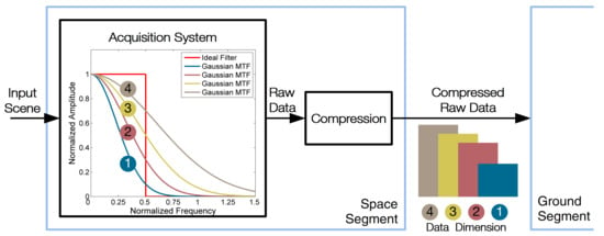
In the real case, the ideal filter is replaced by the system MTF, which can be modeled as a first approximation by a Gaussian function. Obviously, the frequency response of the MTF filter is less selective than the ideal one, and this means that the baseband frequencies will be only partially filtered, as well as the out-of-band frequencies not completely removed. Consequently, the MTF amplitude at the Nyquist frequency gives a measure of the tradeoff between baseband and out-of-band frequencies. Figure 1 compares the frequency responses of the ideal filter and some Gaussian-like MTFs, as a function of the normalized frequency [16]. In the domain of the normalized frequency , the sampling frequency corresponds to the value, whereas the cut-off frequency is equal to . Therefore, Figure 1 must be evaluated for the cut-off frequency . For such normalized frequency, a larger amplitude value of the Gaussian-like MTF implies more spurious out-of-band frequencies. It can be noticed that if the MTF is assumed to be a Gaussian function, the point spread function is also Gaussian.
3. On-Board Data Compression
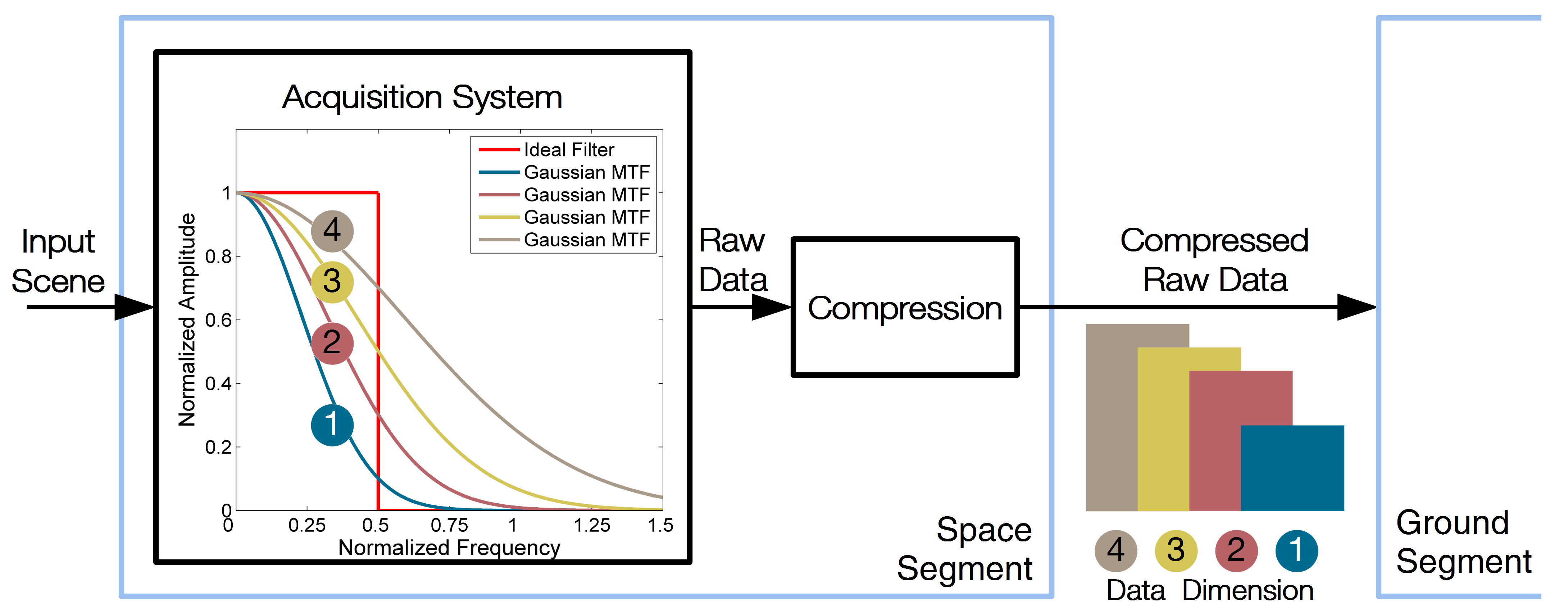
The compression process of the acquired raw data is a mandatory stage in the hyperspectral data process chain, as it is shown in Figure 2. In fact, the transmission load for the hyperspectral data is typically of the order of a Gbyte for each acquired scene.
The most significant indices for assessing the performance of a compression scheme are the BR and the CR. The BR gives the number of bits per pixel of the coded image, so that lower BRs mean better coders. If denotes the total number of bits of the compressed bit stream, and denotes the total number of pixels of the original sequence, we have
A complementary figure is the CR, which must be kept higher as possible. It is defined as the ratio between the total number of bits of the original sequence (), and the total number of bits of the compressed bit stream, that is
with , where is the number of bits per pixel of the original sequence.
If the compression method is not lossless, the algorithm is called lossy. In this case, several error measurements are used in literature to quantify the distance between original and reconstructed 3D data. Even if this work includes only lossless experiments, the RMSE distortion index is here used to compare the simulated data, in the case of an ideal filter and Gaussian-like MTF filters. Let us denote as the reference data set and as the data set to be compared, where , and are the numbers of rows, columns, and bands, respectively, of the reference data set. Let be then the total number of pixels. In this case, the RMSE distortion measure is defined as
where the summation is extended over the whole data set.
A block scheme of a typical compression procedure is shown in Figure 3. The compression stage is essentially composed of two main blocks, which represent the decorrelation and the encoding phases. The decorrelation block performs a transformation of the original data, by producing more uncorrelated samples, which can be more efficiently encoded. To this end, transform-based strategies (as Discrete Wavelet Transform (DWT) [17]), or prediction-based algorithms (as Differential Pulse Code Modulation (DPCM) [18]) can be effectively used. If the former ones are more performing in the lossy case, the latter ones work better if a lossless compression is requested [19,20,21]. In the case of DPCM-like strategies, the possibility to achieve a lossy compression with the additional feature of a peak error controlled by the user is also achievable, by inserting a quantization step in the prediction loop. This is the so-called near-lossless compression, which can be obtained by means of both causal and no-causal schemes [22,23]. Concerning the encoding stage, the arithmetic coding can reach the entropy limit [24], but it is not exploitable for an on-board implementation. Due to their limited complexity, coders working in integer arithmetics, as Golomb-Rice, are adopted instead [25].
Evidently, a lossy algorithm can reach higher CRs, but with the disadvantage of several information losses. The issue is then if a minimization of such a distortion is possible, to achieve decoded data with a sufficient quality [26]. However, in several applications, a lossless compression is mandatory. In this case, DPCM-based strategies are widely used. Lossless DPCM basically consists of a prediction followed by the entropy coding of the differences between original and predicted values (prediction residuals). The prediction is causal in the 3D case, by involving spatially and/or spectrally previously encoded neighbor pixels that are available at the decoder. The predicted value is often computed by considering the neighbors in a linear combination, which can involve both a spatial neighborhood (in the same band) and a spectral one (in several previous bands) [27]. Figure 4 shows a typical spatial/spectral neighborhood for a DPCM scheme, in case two previous spectral bands are used for computing the predicted value. It can be noticed that several different spatial/spectral neighborhoods can be chosen for the prediction, by sequentially considering past values at increasing distances from the current pixel (CP). In Figure 4, pixels at increasing distances are colored by following the attached look-up table. Let us observe that the first considered pixel in the previous bands is the pixel in the same position of the CP. In the particular case of a simple spectral prediction, only the pixels in the same position of the CP are usually considered.
In the on-board scenario, a compression scheme is limited by several constraints, as a low power consumption, the size of the payload, radiation hardening issues, reduced memories, and so on [28]. Consequently, several simplifications are requested, by admitting possible degradations in the performance. Moreover, the on-board algorithm must cope with many noise contributions (striping noise, signal-dependent photonic noise, signal-independent electronic noise). Another important issue is the type of acquisition modality, which does not generally allow an immediate availability of the acquired image in the usual Band Sequential (BSQ) arrangement. In fact, the acquisition is usually done in the Band Interleaved by Line (BIL) and Band Interleaved by Pixel (BIP) modalities. In the case of BSQ, or even of BIL, the spatial correlation is more easily exploitable than in the BIP structure. Consequently, the CR of BIP is less than for BSQ and BIL.
Several low complexity lossless compression algorithms have been proposed in literature to be adopted in the case of on-board requirements [29]. Among them, the Fast Lossless (FL) algorithm [30] has been chosen by CCSDS for the definition of the lossless compression standard CCSDS 1.2.3.0-B-1 for multispectral/hyperspectral data. The definition of this standard is reported in the CCSDS Blue Book [12]. Recently, a novel standard CCSDS 1.2.2.0-B-2 has been defined to specify the modalities for an easy control of the CR in an on-board scenario [31].
CCSDS 1.2.3 Hyperspectral Compression Standard
In this work, the CCSDS 1.2.3 lossless compression standard has been used for the experiments, by resorting to the EMPORDA software [32]. The prediction block of the CCSDS 1.2.3 is rather complicated, but in any case it works in integer arithmetics. A first prediction of the CP is obtained by merging several neighboring pixels in a local sum, which can be computed both in a spatial (possibly only in the vertical direction or even horizontally) and in a spectral order. The local sum is then scaled and refined by exploiting contextual information through several past local differences (also spatial or not) between the already computed predictions and the previous true values [33]. To this end, these differences are weighted by the coefficients of a continuously updated filter. Eventually, a prediction value is computed by employing the local sum and the local differences, in such a way the correspondent residual signed difference is mapped into a non-negative integer by the Prediction Residual Mapper, and successively sent to the Golomb-Rice encoder. This encoder can work by setting the block-adaptive modality or the sample-adaptive modality, which encodes each mapped prediction residual by means of variable-length binary codewords. In this process, an accumulator is used to select the Golomb Power-of-two (GPO2) code parameter [28].
The CCSDS 1.2.3 standard can even switch between two compression modalities, that is, fully and reduced, to cope with different types of data (raw or calibrated) or acquisition arrangements (BSQ, BIL, or BIP). The compression results of this standard over several well-known hyperspectral data sets are reported in [34]. Figure 5 shows a synthetic block scheme of the CCSDS 1.2.3 encoder.
4. Simulation of the Real Acquisition A/D System
Being the acquisition A/D system not available yet, a simulation of the oncoming remote sensed data is required to obtain numerical scores. To this end, a reference image has been employed as the real scene to be acquired, which includes objects whose resolution can be theoretically infinite. Therefore, to perform the procedure correctly, the spatial resolution of the reference image should be much higher than the simulated data. A suitable choice is the airborne Aviris 2006 data set, whose acquired scenes, mainly in the Yellowstone site, are available both in raw and calibrated formats. The raw data of the five Yellowstone scenes are composed by bands, each of them with lines and samples for each line scan. The spatial resolution is 17 m and the spectral resolution is nm, in a spectral range of 380–2500 nm, whereas the radiometric range is bit. The scanner is whisk-broom and acquires data in BIP ordering. In this work, both the scenes 0 and 10 in the raw format have been used in the experiments, due to their different information content.
Figure 6 shows a band in false colors of the original raw Yellowstone scene 0 in BSQ arrangement. Noticeably, the high SNR and negligible striping impairments of this data set makes it optimal for the simulated experiments. To obtain the reduced images, which simulate the future acquisitions, the reference image has been filtered and downsampled by considering several Gaussian filters that simulate the system MTF. To this end, three downsampling factors have been chosen, that is, . Moreover, a 23-taps polynomial filter has been taken as an approximately ideal filter. The frequency response and the coefficients for implementing such a filter can be found in [35], where it is shown that the polynomial filter is approaching an ideal filter. The polynomial filter of [35] is a half-band filter, which has been recursively applied to obtain the requested downsampling factor. In general, a higher downsampling factor allows a more realistic simulation, being the reduced images less affected by the aliasing distortion coming from the reference image. Conversely, a lower downsampling factor implies that the simulated data have a greater spatial resolution, and therefore they are more suitable for the compression experiments. Concerning the cut-off values, they have been taken in a range from to , with a step size equal to .
An unwanted effect of the filtering procedure is that the acquisition noise becomes more correlated, so that it must be recovered in its original form before the compression experiments. By a theoretical point of view, all the possible noise sources should be taken into account in this procedure. In particular, the acquisition process in the imaging spectrometers is responsible for the presence of a considerable signal-dependent contribution due to the photonic noise [36]. Such a noise is particularly challenging in case the useful information of the image must be evaluated [37,38]. However, the high quality of the Aviris 2006 data set allows to simply simulate the original noise by adding a signal-independent contribution, which is characterized by its standard deviation, on the reduced images. In this work, we experimented several standard deviation values as . Let us notice that means no noise added, whereas is a typical project value for the future acquired images.
Simulated Images by Filtering and Downsampling the Reference Image
Figure 7 shows the frequency response of a Gaussian MTF filter, in case the downsampling factor is equal to and the cut-off value is equal to at the Nyquist frequency. Consequently, the sampling frequency of the original acquisition has been divided by four, so that the Nyquist normalized frequency is , that is, a quarter of . A downsampling factor is such that a good approximation is obtained of the ideal scene to be acquired.
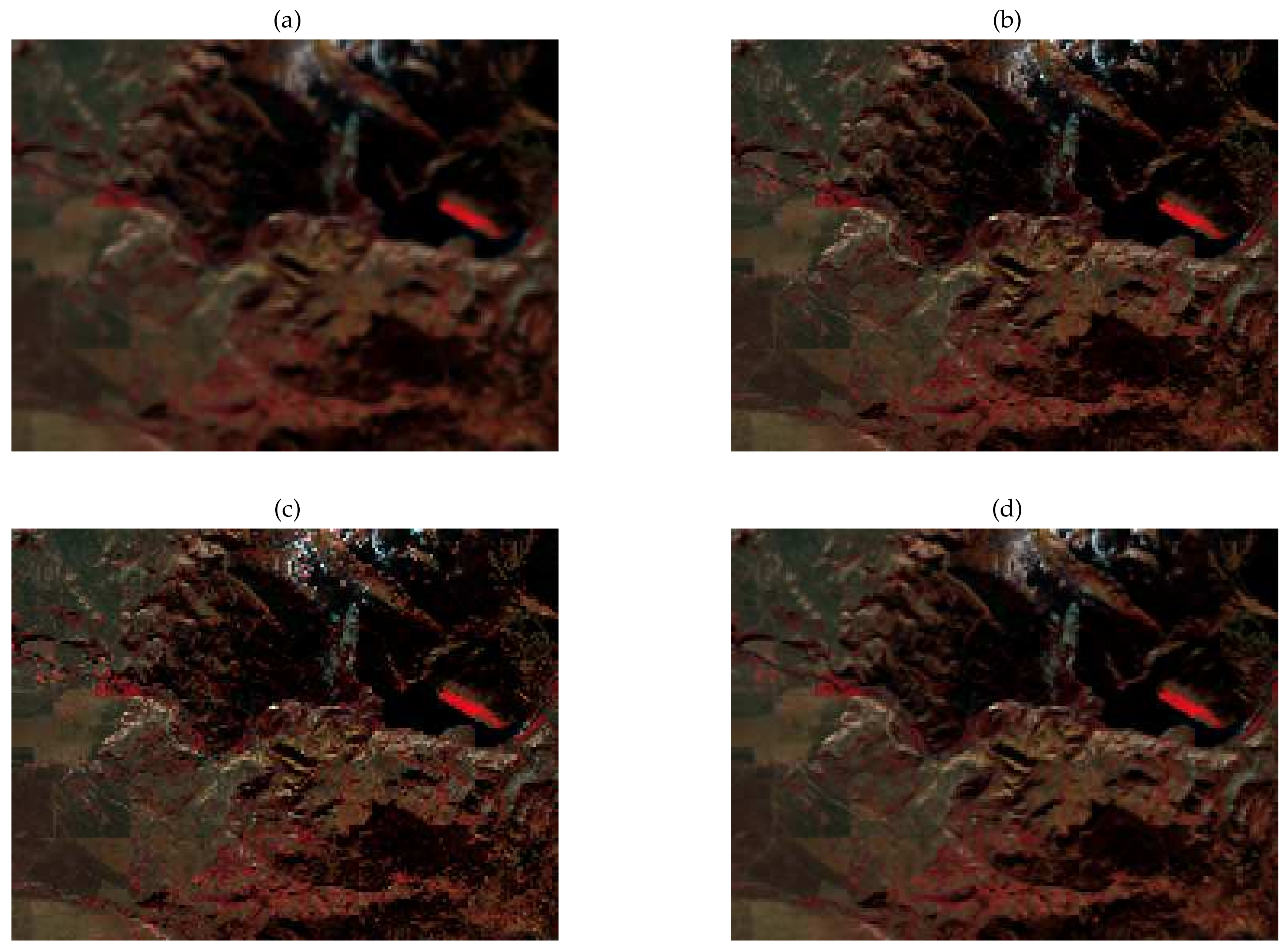
Four downsampled images are shown in Figure 8, by filtering the reference image of Figure 6. In particular, we report the two images filtered by the Gaussian MTFs with the extremal cut-off values and . For comparisons, we also show the image filtered (in two steps) by the 23-taps polynomial approximation of an ideal filter and a simply downsampled image without any filtering. As expected, the image filtered by the MTF with is very smoothed, whereas the image filtered by the MTF with is more informative, even if degraded by evident aliasing distortions. Such impairments are obviously much more noticeable in the unfiltered image. Concerning the polynomial filtered image, it seems to be visually optimal, being an intermediate version between the two Gaussian-like filtered images. Consequently, it can be suitably approximated by keeping the cut-off value in the range .
5. Experimental Results on the CCSDS Aviris 2006 Data Set
The reported experiments on the simulated raw data have been divided in two groups: (a) lossless BR of the reduced Yellowstone scene 0, by varying the image arrangement (BSQ or BIP), the cut-off value of the Gaussian MTF filter, the downsampling factor , and the standard deviation of the signal-independent noise contribution; (b) RMSE versus BR for the Gaussian MTF filtered images in comparison with the image filtered by the 23-taps polynomial kernel, by varying the image arrangement (BSQ or BIP), the cut-off value , the standard deviation , and the scene under investigation. In this case, the downsampling factor has been set to .
5.1. BR Versus the Cut-Off Values
Figure 9 shows the plots of the compression performance (BR versus the cut-off value of the Gaussian MTF filter) for several standard deviation values of the added signal-independent noise. The images are in BSQ format and have been downsampled with a scale factor .
Evidently, the compression algorithm is more efficient if the cut-off value of the MTF filter is low. This happens because the quantity of information of the simulated acquired image is lesser, being the energy of the frequencies in the pass-band lower than for higher cut-off values. The effect of the noise standard deviation is obviously to augment the BR, because a greater number of bits is reserved to encode the noise variability. However, the trends of the plots in Figure 9 tends to become horizontal for high values, that is, the influence of the cut-off value is reduced for a greater noise level. This is due to the spurious compensation of the missing information made by a high noise level, which, however, does not bring any useful information. In particular, for , the BR difference in the range is about one half of bit. For comparison, a dashed line shows the BR of the original data set. The gain of the reduced images is apparent, which is mainly due to the increased data correlation after the filtering process.
Figure 10 shows the same plots of Figure 9, but the processed data are in the BIP format. Let us notice that the plots have been only shifted towards higher BRs, more or less of bpp, whereas the coding of the original image needs about more bpp. This experiment is more realistic than the previous one, because the BIP arrangement is usual in the satellite acquisition process. However, in the following experiments, we use only BSQ data, being the trend of the BIP plots practically the same, with only a constant BR difference, as that reported in Figure 10.
Finally, Figure 11 shows how much the BR is affected by the downsampling factor , by considering the typical noise level . It is apparent that and give equivalent performance, thereby showing the little utility of an excessively reduced spatial resolution. The case is less significant, because the quite similar resolution between the reduced and the reference image, which does not allow a realistic simulation, except for low values. In this case, a BR difference is appreciable, which increases if grows, as expected.
5.2. RMSE Versus BR
Figure 12 reports the relation between BR and RMSE, by varying the cut-off value of the Gaussian MTF filter, when the Gaussian filtered Yellowstone scene 0 is compared with the ideally filtered image. In this case, the standard deviation of the added signal-independent noise is equal to the reference level , and the downsampling factor is . The different values of are shown in Figure 12 in correspondence of the reported curve. The aim of this investigation is to establish which of the MTF filtered images is nearer to the ideally filtered one, if the compression performances are taken as a target. The solution in terms of the distance between the two images (that is, the minimum RMSE) is given by the local minimum of the plot, which is reached for . For such a value, the MTF filtered image is the most similar to the ideally filtered one. If we also take into account the BR, that is, the number of bits required to code the MTF filtered image, the reported plot shows that the cut-off value has an optimal range between and . We can conclude that such an interval includes all the points featuring a satisfactory quality of the MTF filtered image versus acceptable compression performance. Let us notice that the radiometric range of the Aviris 2006 raw data is of 16 bits, so that the range of the RMSE values is proportionally high.
Figure 13 presents several plots, which are similar to the one of Figure 12, but with different standard deviations of the noise added to the filtered images before compression. Evidently, the addition of more signal-independent noise contributions does not substantially change the trend of the plot in Figure 12. However, it can be noticed that the greater is the noise standard deviation, and the more peaked is the correspondent curve. This happens because the introduction of a high noise level makes more critical the compression stage, whose optimal working point tends to become unstable.
As a final experiment, Figure 14 highlights the compression performance (RMSE versus BR) when two different scenes of the Aviris 2006 Yellowstone site are coded, that is, scene 0 and scene 10. These scenes have been chosen because of the large gap of the respective information content. Consequently, the difference of their compression performance is maximized, as it is clearly shown by Figure 14. In particular, the plot of the more informative data set (e.g., scene 0) appears to be shifted towards both greater BR and RMSE. This could be easily foreseen, because the difference between the compression results of the MTF-based and ideally filtered images grows if the scene under investigation is more difficult to be coded. As in the case of a high noise level in Figure 13, the plot of scene 0 is more peaked, which implies a faster drift from the optimal minimum point.
5.3. Computational Performance
The aim of this work is not to propose a novel on-board compression algorithm, but only to investigate how the compression performance change, by varying the MTF of the acquisition system, in case a standard compression scheme, as the CCSDS 1.2.3 hyperspectral/multispectral standard, is used. Consequently, an investigation on the strategies for optimizing the computational performance for an on-board implementation, especially by means on a FPGA, is outside the scope of this paper. In any case, a detailed discussion on such a topic can be found in [39]. In this work, the compression and decompression stages have used a JAVA version of the EMPORDA software featuring the standard CCSDS 1.2.3 algorithm. The software has been implemented on a Linux workstation with a CPU AMD Phenom II X4 955 3.2GHz with a RAM of 8GB.
6. Concluding Remarks and Future Developments
This work has investigated and quantified the influence of the system MTF on the real-time on-board compression of hyperspectral raw data, especially focusing on the case of future missions on mini-satellites. To this end, a reference image has been taken for simulating the analog scene to be acquired, then a filtering and downsampling procedure has generated the simulated acquired images. To perform a correct analysis, several different signal-independent noise levels have been added to the simulated images, in such a way the noise level of the real acquired data can be recovered. The compression of the simulated images, by adopting the well-known CCSDS 1.2.3 lossless multispectral/hyperspectral standard, has shown that the BR of the simulated data increases when the cut-off values grow, as expected. Noticeably, an optimal range of cut-off values has been determined, which allows a good tradeoff between the quality of the acquired image and the lossless compression performance. Such a range has been extensively found between and , which give a range of CRs in BIP format between and . Within this interval, the optimal point could be taken at the middle point . However, by considering manufacturing constraints and a better CR, a suggested cut-off value can be . In the case of BIP format, such a choice gives a CR of about , which is an acceptable score. As a final observation, the reported analysis can be efficiently used for determining the optimal cut-off value for each system MTF. In fact, the proposed methodology is quite flexible and therefore suitable for different spatial resolutions, cut-off values, and MTF shapes. In the future, such an analysis could be refined once the acquisition parameters of some upcoming mini-satellite missions, as the one foreseen by the SMART project, were available.
Author Contributions
B.A. wrote the article, also by integrating all the contributions. M.S. wrote the MTF contribution, and made the figures. M.S. and A.A. managed the data sets and performed the experiments. S.B. supervised all the work from theoretical and practical point of views.
Funding
This research has been developed in the framework of the SMART (Spettrometro Miniaturizzato Avanzato per Ricerca Tecnologica) Project, supported by the Regional Operative Program POR - FESR 2014-2020 funded by Tuscany Region, Italy (Call RS 2017).
Acknowledgments
The authors are grateful to the NASA space agency for providing the Aviris raw data (https://aviris.jpl.nasa.gov/alt_locator). They are also very grateful to Ian Blanes for kindly providing the EMPORDA software, which is available at the site http://deic.uab.cat.
Conflicts of Interest
The authors declare no conflicts of interest.
References
- Magli, E.; Olmo, G.; Quacchio, E. Optimized onboard lossless and near-lossless compression of hyperspectral data using CALIC. IEEE Geosci. Remote Sens. Lett. 2004, 1, 21–25. [Google Scholar] [CrossRef]
- Aiazzi, B.; Alparone, L.; Baronti, S.; Lastri, C. Crisp and fuzzy adaptive spectral predictions for lossless and near-lossless compression of hyperspectral imagery. IEEE Geosci. Remote Sens. Lett. 2007, 4, 532–536. [Google Scholar] [CrossRef]
- Rasti, B.; Scheunders, P.; Ghamisi, P.; Licciardi, G.; Chanussot, J. Noise reduction in hyperspectral images: Overview and application. Remote Sens. 2018, 10, 482. [Google Scholar] [CrossRef]
- Nikolova, I. Micro-satellites advantages. Profitability and return. In Proceedings of the SES 2005, International Scientific Conference Space, Ecology, Safety, Varna, Bulgaria, 10–13 June 2005. [Google Scholar]
- Agenzia Spaziale Italiana (ASI). Italian Space Agency Perspective on Small Satellites; ASI: Roma, Italy, 2016. [Google Scholar]
- Giunta Regionale Toscana. Programma Operativo Regionale FESR 2014–2020; Giunta Regionale Toscana: Toscana, Italy, 2017. [Google Scholar]
- Aiazzi, B.; Alparone, L.; Baronti, S.; Carlà, R. An assessment of pyramid-based multisensor image data fusion. Image Signal Process. Remote Sens. 1998, 3500, 237–249. [Google Scholar]
- Eckardt, A.; Reulke, R. On the design of high resolution imaging systems. Int. Arch. Photogramm. Remote Sens. Spat. Inf. Sci. 2017, 42, 97–100. [Google Scholar] [CrossRef]
- Vollmerhausen, R.H.; Driggers, R.G. Analysis of Sampled Imaging Systems; SPIE Publication: Bellingham, WA, USA, 2000. [Google Scholar]
- Pu, R. Hyperspectral Remote Sensing: Fundamentals and Practices; CRC Press: Boca Raton, FL, USA, 2017. [Google Scholar]
- Aiazzi, B.; Baronti, S.; Selva, M.; Alparone, L. Bi-cubic interpolation for shift-free pan-sharpening. ISPRS J. Photogramm. Remote Sens. 2013, 86, 65–76. [Google Scholar] [CrossRef]
- Consultative Committee for Space Data Systems. Lossless Multispectral and Hyperspectral Image Compression—Recommended Standard (Blue Book); Consultative Committee for Space Data Systems: Washington, DC, USA, 2012. [Google Scholar]
- Coppo, P.; Chiarantini, L.; Alparone, L. Design and validation of an end-to-end simulator for imaging spectrometers. Opt. Eng. 2012, 51, 1–14. [Google Scholar] [CrossRef]
- Coppo, P.; Chiarantini, L.; Alparone, L. End-to-end image simulator for optical imaging systems: Equations and simulation examples. Adv. Opt. Technol. 2013, 2013, 295950. [Google Scholar] [CrossRef]
- Boreman, G.D. Modulation Transfer Function in Optical and Electro-Optical Systems; SPIE Publication: Bellingham, WA, USA, 2001. [Google Scholar]
- Alparone, L.; Aiazzi, B.; Baronti, S.; Garzelli, A. Spatial methods for multispectral pansharpening: Multiresolution analysis demystified. IEEE Trans. Geosci. Remote Sens. 2016, 54, 2563–2576. [Google Scholar] [CrossRef]
- Shensa, M.J. The discrete wavelet transform: Wedding the à trous and Mallat algoritm. IEEE Trans. Signal Process. 1992, 40, 2464–2482. [Google Scholar] [CrossRef]
- Ke, L.; Marcellin, M.W. Near-lossless image compression: Minimum entropy, constrained-error DPCM. IEEE Trans. Image Process. 1998, 7, 225–228. [Google Scholar] [PubMed]
- Aiazzi, B.; Alba, P.; Alparone, L.; Baronti, S. Lossless compression of multi/hyper-spectral imagery based on a 3-D fuzzy prediction. IEEE Trans. Geosci. Remote Sens. 1999, 37, 2287–2294. [Google Scholar] [CrossRef]
- Aiazzi, B.; Alparone, L.; Baronti, S. Fuzzy logic-based matching pursuits for lossless predictive coding of still images. IEEE Trans. Fuzzy Syst. 2002, 10, 473–483. [Google Scholar] [CrossRef]
- Aiazzi, B.; Baronti, S.; Alparone, L. Lossless compression of hyperspectral images using multiband lookup tables. IEEE Signal Proc. Lett. 2009, 16, 481–4844. [Google Scholar] [CrossRef]
- Aiazzi, B.; Alparone, L.; Baronti, S. Near-lossless image compression by relaxation-labelled prediction. Signal Process. 2002, 82, 1619–1631. [Google Scholar] [CrossRef]
- Aiazzi, B.; Alparone, L.; Baronti, S.; Santurri, L.; Selva, M. Information-theoretic assessment of on-board near-lossless compression of hyperspectral data. J. Appl. Remote Sens. 2013, 7, 074597. [Google Scholar] [CrossRef]
- Witten, I.H.; Neal, R.M.; Cleary, J.G. Arithmetic coding for data compression. Commun. ACM 1987, 30, 520–540. [Google Scholar] [CrossRef]
- Rice, R.F.; Plaunt, J.R. Adaptive variable-length coding for efficient compression of spacecraft television data. IEEE Trans. Commun. Technol. 1971, COM-19, 889–897. [Google Scholar] [CrossRef]
- Aiazzi, B.; Alparone, L.; Baronti, S.; Lastri, C.; Selva, M. Spectral distortion in lossy compression of hyperspectral data. J. Electr. Comput. Eng. 2012, 2012, 850637. [Google Scholar] [CrossRef]
- Aiazzi, B.; Alparone, L.; Baronti, S. Near-lossless compression of 3-D optical data. IEEE Trans. Geosci. Remote Sens. 2001, 39, 2547–2557. [Google Scholar] [CrossRef]
- Blanes, I.; Magli, E.; Serra-Sagristà, J. A tutorial on image compression for optical space imaging systems. IEEE Geosci. Remote Sens. Mag. 2014, 2, 8–26. [Google Scholar] [CrossRef]
- Aiazzi, B.; Alparone, L.; Baronti, S. On-board DPCM compression of hyperspectral data. In Proceedings of the ESA OBPDC 2010, 2nd International Workshop on On-Board Payload Data Compression, Toulouse, France, 28–29 October 2010; pp. 1–8. [Google Scholar]
- Klimesh, M.A. Low-complexity adaptive lossless compression of hyperspectral imagery. Satell. Data Compr. Commun. Arch. II 2006, 6300, 63000N. [Google Scholar]
- Consultative Committee for Space Data Systems. Image Data Compression–Recommended Standard (Blue Book); Consultative Committee for Space Data Systems: Washington, DC, USA, 2017. [Google Scholar]
- Auge, E.; Santalo, J.; Blanes, I.; Serra-Sagrista, J.; Kiely, A. Review and implementation of the emerging CCSDS recommended standard for multispectral and hyperspectral lossless image coding. In Proceedings of the CCP 2011, IEEE 1st International Conference on Data Compression, Communication and Processing, Palinuro, Italy, 21–24 June 2011; pp. 229–235. [Google Scholar]
- Aiazzi, B.; Alparone, L.; Baronti, S. Context modeling for near-lossless image coding. IEEE Signal Process. Lett. 2002, 9, 77–80. [Google Scholar] [CrossRef]
- Consultative Committee for Space Data Systems. Lossless Multispectral and Hyperspectral Image Compression—Informational Report (Green Book); Consultative Committee for Space Data Systems: Washington, DC, USA, 2015. [Google Scholar]
- Aiazzi, B.; Alparone, L.; Baronti, S.; Garzelli, A. Context-driven fusion of high spatial and spectral resolution images based on oversampled multiresolution analysis. IEEE Trans. Geosci. Remote Sens. 2002, 40, 2300–2312. [Google Scholar] [CrossRef]
- Aiazzi, B.; Alparone, L.; Baronti, S.; Selva, M.; Stefani, L. Unsupervised estimation of signal-dependent CCD camera noise. Eur. J. Adv. Signal Process. 2012, 2012, 231. [Google Scholar] [CrossRef]
- Aiazzi, B.; Alparone, L.; Barducci, A.; Baronti, S.; Pippi, I. Estimating noise and information of multispectral imagery. Opt. Eng. 2002, 41, 656–668. [Google Scholar]
- Alparone, L.; Selva, M.; Aiazzi, B.; Baronti, S.; Butera, F.; Chiarantini, L. Signal-dependent noise modelling and estimation of new-generation imaging spectrometers. In Proceedings of the WHISPERS 2009, 1st IEEE Workshop on Hyperspectral Image and Signal Processing: Evolution in Remote Sensing, Grenoble, France, 26–28 August 2009. [Google Scholar]
- Báscones, D.; González, C.; Mozos, D. Parallel Implementation of the CCSDS 1.2.3 Standard for Hyperspectral Lossless Compression. Remote Sens. 2017, 9, 973. [Google Scholar] [CrossRef]
Figure 1.
Frequency responses of some Gaussian-like MTFs versus the ideal filter.

Figure 2.
Hyperspectral data analysis chain. The compression stage is mandatory in the space segment.
Figure 2.
Hyperspectral data analysis chain. The compression stage is mandatory in the space segment.

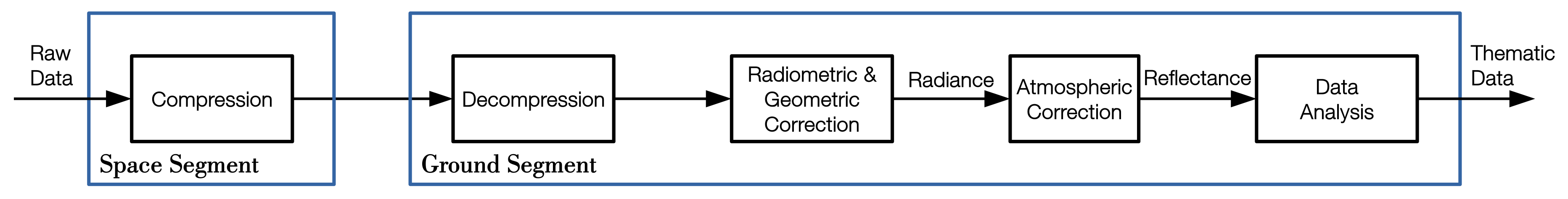
Figure 3.
A typical procedure showing the compression and decompression stages.

Figure 4.
Spatial/spectral neighborhoods in a DPCM scheme.

Figure 5.
Block scheme of the lossless compression CCSDS 1.2.3 standard.

Figure 6.
A band in false colors of the original raw Yellowstone scene 0 of the Aviris 2006 data set.
Figure 6.
A band in false colors of the original raw Yellowstone scene 0 of the Aviris 2006 data set.

Figure 7.
Frequency response of a Gaussian-like MTF filter in the case of and .

Figure 8.
Simulated images filtered by: (a) Gaussian MTF with ; (b) Gaussian MTF with ; (c) All-pass filter; (d) 23-taps polynomial filter.
Figure 8.
Simulated images filtered by: (a) Gaussian MTF with ; (b) Gaussian MTF with ; (c) All-pass filter; (d) 23-taps polynomial filter.

Figure 9.
BR versus by varying for the Yellowstone scene 0 in BSQ format.

Figure 10.
BR versus by varying for the Yellowstone scene 0 in BIP format.

Figure 11.
BR versus by varying for the Yellowstone scene 0 in BSQ format.

Figure 12.
RMSE versus BR by varying for the Yellowstone scene 0 in the BSQ format.

Figure 13.
RMSE versus BR by varying and , for the Yellowstone scene 0 in the BSQ format.

Figure 14.
RMSE versus BR by varying for the Yellowstone scene 10 in the BSQ format.

© 2019 by the authors. Licensee MDPI, Basel, Switzerland. This article is an open access article distributed under the terms and conditions of the Creative Commons Attribution (CC BY) license (http://creativecommons.org/licenses/by/4.0/).
Share and Cite
MDPI and ACS Style
Aiazzi, B.; Selva, M.; Arienzo, A.; Baronti, S. Influence of the System MTF on the On-Board Lossless Compression of Hyperspectral Raw Data. Remote Sens. 2019, 11, 791. https://doi.org/10.3390/rs11070791
AMA Style
Aiazzi B, Selva M, Arienzo A, Baronti S. Influence of the System MTF on the On-Board Lossless Compression of Hyperspectral Raw Data. Remote Sensing. 2019; 11(7):791. https://doi.org/10.3390/rs11070791
Chicago/Turabian StyleAiazzi, Bruno, Massimo Selva, Alberto Arienzo, and Stefano Baronti. 2019. "Influence of the System MTF on the On-Board Lossless Compression of Hyperspectral Raw Data" Remote Sensing 11, no. 7: 791. https://doi.org/10.3390/rs11070791
Note that from the first issue of 2016, this journal uses article numbers instead of page numbers. See further details here.