Spatio-Temporal Patterns of Land Use/Land Cover Change in the Heterogeneous Coastal Region of Bangladesh between 1990 and 2017

Abstract

Although a detailed analysis of land use and land cover (LULC) change is essential in providing a greater understanding of increased human-environment interactions across the coastal region of Bangladesh, substantial challenges still exist for accurately classifying coastal LULC. This is due to the existence of high-level landscape heterogeneity and unavailability of good quality remotely sensed data. This study, the first of a kind, implemented a unique methodological approach to this challenge. Using freely available Landsat imagery, eXtreme Gradient Boosting (XGBoost)-based informative feature selection and Random Forest classification is used to elucidate spatio-temporal patterns of LULC across coastal areas over a 28-year period (1990–2017). We show that the XGBoost feature selection approach effectively addresses the issue of high landscape heterogeneity and spectral complexities in the image data, successfully augmenting the RF model performance (providing a mean user’s accuracy > 0.82). Multi-temporal LULC maps reveal that Bangladesh’s coastal areas experienced a net increase in agricultural land (5.44%), built-up (4.91%) and river (4.52%) areas over the past 28 years. While vegetation cover experienced a net decrease (8.26%), an increasing vegetation trend was observed in the years since 2000, primarily due to the Bangladesh government’s afforestation initiatives across the southern coastal belts. These findings provide a comprehensive picture of coastal LULC patterns, which will be useful for policy makers and resource managers to incorporate into coastal land use and environmental management practices. This work also provides useful methodological insights for future research to effectively address the spatial and spectral complexities of remotely sensed data used in classifying the LULC of a heterogeneous landscape.

1. Introduction

An accurate estimation of land use/land cover change (LULCC) is essential for improved understanding of its impacts on climatic and environmental systems, to enable the implementation of appropriate environmental management practices [1]. The changing climate and its multifaceted, multi-scaled ramifications (e.g., sea-level rise, frequent storm surges) pose tremendous challenges to the coastal regions of Bangladesh, which include salinity intrusion, loss of vegetation, and loss of agricultural productivity. In addition to frequent natural disturbances, these regions have been subjected to rapid urbanization and economic development. An estimated 35 million people currently live in the coastal belt of Bangladesh [2,3], with associated activities causing significant alteration to the coastal land cover features at various spatial and temporal scales [4]. These changes, for the most part driven by anthropogenic activities, contribute to the loss of ecosystem services to an increased risk of natural hazards. Therefore, to identify effective strategies for dealing with the existing challenges, a detailed investigation of coastal LULCC dynamics has become indispensable for resource managers and planners. Although the LULCC research goes back decades, it is surprising that a comprehensive picture regarding such changes in coastal Bangladesh is still lacking, primarily due to the poor quality of accessible remotely sensed data over what is a highly complex, heterogeneous coastal landscape. This, in turn, poses unique challenges for large-scale data processing and analyses.

The coastal region of Bangladesh constitutes a large area (~710 km coastline) with a high degree of landscape diversity with the presence of human settlements, flat and hilly topography, forests, numerous tidal flats and creeks, natural levees, estuaries, mangrove swamps, muddy flats and sandy beaches [3,5,6]. The challenges involved in the accurate classification of LULC across such a complex, heterogeneous biophysical landscape (e.g., coastal region of Bangladesh) arise from three major factors. First, the classification of LULC is highly susceptible to generalization and information loss due to the spatial and spectral limitations of available image data. Existing medium to low-resolution imageries provided by Landsat (30 m) are perhaps a perfect example. Mixed pixels in these images can lead to spectral confusion and problems in differentiating various land use categories. Studies suggest that even sub-meter spatial resolution images are not capable of explaining inter- and intra-class variability in a heterogeneous landscape [7]. Second, images with coarse temporal granularity are not ideal for a detailed understanding of LULCC dynamics in regions that are under rapid and indiscriminate or unsystematic manipulation. Third, spectral complexities of the image objects are introduced due to various unfavorable local environmental and weather conditions (e.g., presence of thick dust, haze, and clouds), and large-scale biophysical changes, resulting from environmental disturbances (e.g., tropical cyclones) [8,9]. These systematic and non-systematic factors introduce substantial challenges in reliably depicting spatio-temporal (space-time) patterns of LULCC in large geo-spaces when applying an algorithmic image classification process.

Thematic mapping of LULC is commonly based on a number of image classification techniques [10]. To date, the most widely used classification methods and associated algorithms fall into a number of categories—supervised and unsupervised, parametric and nonparametric, hard and soft (fuzzy) classification, or per-pixel, subpixel and per field categories (for a comprehensive review, see Lu and Weng, 2007). Among those, the most heavily used image classification methods are maximum likelihood classifier (MLC), K-Means, and ISODATA. However, MLC is a parametric approach and therefore performs accurately when spectral data are normally distributed. This tends not to be the case for image data for the coastal region of Bangladesh, which exhibit a non-linear distribution of landscape features. Due to the fact that these are unsupervised techniques, K-Means and ISODATA are often undesirable because they do not allow expert knowledge input (e.g., labeling of clusters) into the LULC map generation process. To tackle these challenges, previous research has adopted advanced classification algorithms including artificial neural networks (ANN), Support Vector Machines (SVM), Random Forest (RF), and Classification and Regression Trees (CART) [11,12]. RF and SVM algorithms are the most popular in the RS community [13,14] and are widely used for multispectral and hyperspectral image classification tasks. These classifiers outperform traditional parametric approaches with their ability to deal with noise, discrete/continuous as well as unbalanced datasets [15]. RF’s LULC classification accuracy is comparable to other ensemble learning techniques—namely, bagging and boosting [16,17]. Besides high accuracy, RF has robustness against overfitting on the training data and requires considerably less tuning of the parameters than boosting ensembles, and provides measure of variable importance that can be used for the final model development. Despite these positive features, RF’s performance can be limited when classifying the LULC of a heterogeneous landscape, since RF’s randomized bagging-based feature selection and classification approach can be biased towards the majority class and therefore, can misclassify the minority class within the data [18,19]. Another point to note is that, for coastal areas comprised of sandy beaches, rivers, patchy inland swamps and forest canopy layer, an image pixel of moderate spatial resolution can encompass multiple features on the ground. This can lead to a similarity in spectral reflectance among multiple features, especially in urban/built-up areas. RF’s important feature selection approach is less reliable when predictor features are correlated with each other, and therefore can perform poorly in identifying most informative features—i.e., spectral bands that are most discriminative among LULC classes [20]. In such cases, a separate stage of feature selection prior to the model building process can be used for achieving improved predictive performance of the RF classifier.

For reliable LULC mapping, selection of appropriate remotely sensed datasets and choice of a suitable classification system are considered the two most important factors [10]. Yet, the use of 30-m resolution Landsat images is the only viable option for LULC classification for coastal region in Bangladesh. Therefore, landscape heterogeneity and complexities inherent within existing image data, in regards to spatial, radiometric, spectral, and temporal properties, warrant careful selection of procedures to be used in a typical LULC mapping workflow: image processing, training sample generation, feature extraction and selection, choice of appropriate classification method, post-classification processing, and accuracy assessment.

Feature extraction/selection is a critical step in the image classification task, as often only a few features (e.g., spectral bands) in a multispectral or hyperspectral image contain meaningful information necessary for separating individual LULC classes (e.g., pond vs. mangrove swamps). The most common feature extraction method is principal component analysis (PCA), which transforms the data into a new set of principle components that best describe the underlying structure of the original dataset [21]. Other feature extraction methods are minimum noise fraction transform, discriminant analysis, decision boundary feature extraction, non-parametric weighted feature extraction, wavelet transform, and spectral mixture analysis [10]. Feature selection involves finding a subset of features in the dataset that contribute most to the accuracy of a classification model. Common feature selection approaches include wrappers, embedded methods, semantic groupings, and filters. The wrappers approach makes use of the learning algorithm itself to evaluate various subsets of features during the classification process, but it has a high risk of overfitting and is also computationally intensive [22]. Although inherently similar to the wrappers, the embedded feature selection techniques (e.g., LASSO regularization and Decision Trees) utilize an intrinsic model-building metric to determine (learn) which features contribute the most to the classification accuracy. While the LASSO feature selection algorithm performs well in modeling linear correlations between features, it cannot determine non-linear feature dependencies [23]. Semantic groupings involve selection of features (e.g., spectral or texture features) based on their type or by expert opinion. Filter feature selection methods use a pre-processing step, which is independent of the learning algorithm; they apply a statistical measure (e.g., Chi square test, information gain, and correlation coefficient scores) to rank each feature by the determined score. Classification and Regression Trees (CART) and Random Forest (RF) are two of the popular filter methods that are commonly used in most of the remote sensing applications. CART is a decision tree (DT)-based learning algorithm that uses binary recursive partitioning to grow DTs, using Gini and Twoing methods that search for important relationships and patterns in the data. CART feature selection was successfully used for vegetation and crop classification in moderate to high spatial resolution imageries (e.g., multi-temporal MODIS) [24,25].

A Random Forest constructs an ensemble model of decision trees from random subsets of features and bagged samples of the training data [15]. Like CART, RFs were used for feature selection leading to improved classification accuracy in mapping land-cover [8,9] and crops [26]. However, both CART and RF can perform poorly for high-dimensional and unbalanced data; recursive binary splitting and the bagging randomization process involved in these algorithms can be biased toward uninformative features [27,28]. Extreme gradient boosting (XGBoost)—another filter-based feature selection algorithm started gaining popularity recently [29,30,31]. XGBoost is a new implementation of boosting CART algorithms that improves the accuracy of classification through iterative computation of weak (basic) classifiers. It usually outperforms benchmark classifiers such as support vector machines (SVM) or RF, and thus has gained much popularity in the Machine Learning community—particularly in Kaggle competitions, and most recently in image classification [32,33,34,35]. In identifying important features, the XGBoost algorithm uses boosted trees to obtain feature scores. The more a feature is used for devising key decisions with boosted trees, the greater the score assigned to that feature. This approach can thus reduce class bias. XGBoost also utilizes the “sparsity-aware split finding” approach that can be highly advantageous for data with heterogeneously distributed features space, as usually manifested in the remotely sensed data of complex and heterogeneous coastal landscapes of Bangladesh. Moreover, the XGBoost algorithm employs measures of gain, frequency, and cover, that can deal with correlation among features while searching for the most important or discriminative features [30].

A few studies exist that shed light on LULC change in the coastal areas of Bangladesh. While these studies highlight the space-time dynamic of coastal land-use, they are limited in geographic scope—i.e., focused on a relatively small coastal area comprising a few districts [4,12,36] or specific agro-ecological regions [3]. As such, the existing literature does not provide a detailed, comprehensive understanding on the changing pattern of LULC across the entire coastal region. To overcome this identified research gap, this study took up the challenge to produce detailed, multi-year LULC maps of the entire coastal region of Bangladesh, with an aim to provide insight into the varied level of interplays that exist between human and the physical environment in this region. In doing so, this study employed a unique methodological approach compared to those found in existing studies—that is, it quantified multi-year coastal LULC classes using two state-of-the-art machine learning algorithms—XGBoost and Random Forest. Specifically, using these advanced algorithms, this study evaluated the performance of an integrated feature selection and classification modeling approach for LULC classification in a large and heterogeneous coastal landscape. Consequently, this study sought to answer two specific contextual and methodological questions, as follows:

• What are the multi-year spatial and temporal patterns of LULC in the heterogeneous coastal region of Bangladesh?
• Does the XGBoost feature selection contribute to an improved performance of the RF algorithm for LULC classification in a highly heterogeneous landscape?

2. Materials and Methods

2.1. Description of the Study Area

The study area covers the entire coastal region of Bangladesh (Figure 1), an area of 4,625,334 hectares of coastal floodplains [5,37]. The region is comprised of nineteen districts and is characterized by an extremely hydrologically active geomorphic setting, with elevation ranging from 0 to 986 m above the mean sea-level. There are numerous tidal rivers that infrequently inundate the inlands and cause waterlogging. Furthermore, the conical shape of the study area and the lower elevation compared to that of the sea cause a backwater effect and contribute heavily to waterlogging issues [38]. Due to the region’s close proximity to the Bay of Bengal, salinity levels in the soil and river systems are also considerably higher than in any part of the country [37,39,40]. The southwestern part of the region is covered by a dense mangrove forest, known as the Sundarbans, which offers a natural protection to most of the natural disasters, particularly from cyclones developed in the sea [41]. The flora and fauna of the Sundarbans are considered to be a part of the World Heritage sites and are critical for maintaining the ecological well-being of the coastal area [42]. The Sundarbans is one of the most unique mangrove forests in the world and can be highly susceptible to any unplanned land use and land cover changes [43,44].

The mean annual temperature in the area is 33.74 °C with a precipitation of 177.21 cm/year [45]. The people inhabiting this area are mainly involved in the primary activities (e.g., farming, fishing) for sustenance, which make them vulnerable to any adverse environmental processes [5]. In the past, people have migrated away from this region due to cyclones, storm surges and other natural disasters [46] that account for the stunted development of the region [47,48]. The high population density in this region has also led to the exploitation of the newly formed islands (locally known as Chars), an issue which also strongly contributes to LULC changes along the coastal areas of Bangladesh [39].

2.2. Data Acquisition and Preparation

Figure 2 shows the overall workflow of this study. The data preparation phase started with the acquisition of eight Landsat TM and OLI-TIRS scenes (at 30 x 30m resolution), covering the entire coastal regions of Bangladesh for individual years including 1990, 1995, 2000, 2005, 2010, and 2017. As a result, a total of forty-eight images between 1990 and 2017 were used. To minimize atmospheric disturbances in the datasets, only dry season images with less than 5% cloud cover were obtained. Radiometric corrections were performed through the conversion of raw digital numbers to top-of-atmosphere (TOA) reflectance [49]. Atmospheric corrections were performed to remove the remaining atmospheric disturbances (e.g., haze) through identification of the darkest pixel value in each band and the subsequent subtraction of this value from every pixel [50].

Multi-temporal Google Earth aerial imageries were used to select suitable training sites from the acquired Landsat images and to collect training pixels/areas related to six LULC types (

Table 1. Land cover classification scheme used in this study.

LULC Class	Description
Built-up	Residential, commercial and services, industrial, transportation, roads, mixed urban, and other urban
Bare soil	Exposed soils, construction sites
Agricultural land	Cultivated land, crop fields, fallow lands, and vegetable fields
Vegetation	Deciduous forest, mixed forest lands, palms, conifer, scrub, and others
Wetland	Permanent and seasonal wetlands, inland water bodies, low-lying areas, marshy land, rills and gully, swamps
River	River networks, canals and active hydrological features

) using photo-interpretation techniques. On average, 850 training samples were collected for use in the LULC classification. Data for model training and LULC classification were selected while maintaining a uniform distribution among the feature classes and a homogeneous distribution over the study area (i.e., maintaining an equal number of training points for each class spread homogenously over the study area). However, it should be noted that dry season (e.g., November and December) rice (locally called “Boro” paddy) cultivation and associated waterlogging via irrigation in many coastal areas offered substantial challenges in isolating agricultural and wetland areas, even via geolinked Google Earth imageries. Moreover, existing Google Earth imageries corresponding to the study area in 1990, 1995 and 2000 are not as clear as the recent years (i.e., 2005, 2010 and 2017). This is noticeable when attempting the accurate identification of areas related to small urban patches, agricultural lands, and inland water bodies. Hence, multi-year normalized differential vegetation index (NDVI), normalized difference water index (NDWI), and normalized difference built-up index (NDBI) were produced to assist in the training data generation process. Training data showing an agreement with these three indices and the imagery available in Google Earth, were finally retained for mapping LULC.

2.3. Feature Selection Process

It is important to use only image features (i.e., spectral bands) that are most useful for accurately separating different LULC classes.

Table 2. Correlation matrices showing Pearson correlation coefficients between image features (i.e., spectral bands) for individual years. Values in bold face show the correlation between the bands used for the final RF classification.

Year	Band	B1	B2	B3	B4	B5	B6	B7
1990	TM 1	1
	TM 2	0.922 **	1
	TM 3	0.845 **	0.952 **	1
	TM 4	−0.029	0.018	0.001	1
	TM 5	0.089 *	0.155 **	0.245 **	0.782 **	1
	TM 6	0.181 **	0.241 **	0.359 **	0.591 **	0.951 **	1
1995	TM 1	1
	TM 2	0.953 **	1
	TM 3	0.887 **	0.947 **	1
	TM 4	−0.284 **	−0.250 **	−0.232 **	1
	TM 5	−0.031	0.032	0.189 **	0.708 **	1
	TM 6	0.112 *	0.181 **	0.362 **	0.506 **	0.954 **	1
2000	TM 1	1
	TM 2	0.969 **	1
	TM 3	0.961 **	0.984 **	1
	TM 4	−0.268 **	−0.255 **	−0.312 **	1
	TM 5	−0.037	−0.049	−0.073	0.825 **	1
	TM 6	0.241 **	0.209 **	0.210 **	0.573 **	0.913 **	1
2005	TM 1	1
	TM 2	0.957 **	1
	TM 3	0.841 **	0.938 **	1
	TM 4	0.366 **	0.361 **	0.380 **	1
	TM 5	0.268 **	0.348 **	0.513 **	0.794 **	1
	TM 6	0.273 **	0.382 **	0.575 **	0.652 **	0.963 **	1
2010	TM 1	1
	TM 2	0.922 **	1
	TM 3	0.799 **	0.919 **	1
	TM 4	0.047	0.102 **	0.160 **	1
	TM 5	0.156 **	0.292 **	0.503 **	0.741 **	1
	TM 6	0.202 **	0.347 **	0.574 **	0.524 **	0.941 **	1
2017	OLI 1	1
	OLI 2	0.981 **	1
	OLI 3	0.896 **	0.951 **	1
	OLI 4	0.761 **	0.856 **	0.930 **	1
	OLI 5	0.075 *	−0.023	−0.011	−0.089 **	1
	OLI 6	0.221 **	0.202 **	0.247 **	0.355 **	0.730 **	1
	OLI 7	0.290 **	0.312 **	0.362 **	0.527 **	0.474 **	0.936 **	1

** Correlation is significant at the 0.01 level. * Correlation is significant at the 0.05 level.

shows the outcome of an exploratory analysis; the Pearson correlation statistic was employed to reveal the statistically significant pairwise associations between spectral bands corresponding to multi-temporal images used in this study. Hence, the XGBoost algorithm was used to select important features (i.e., spectral bands) that were used later for LULC classification using the RF algorithm. We implemented the XGBoost feature selection process using the ‘xgboost’ package in R. The XGBoost algorithm was built as an enhanced version of the gradient boosting decision tree algorithm (GBDTA) [30,31]. GBDTA is a regression and classification technique that develops prediction models based on weak prediction models—the decision trees. The term ‘weak’ or ‘strong’ refers to the measure of how weakly or strongly the classification learners are correlated in relation to the actual target variable. Based on errors, the process progressively assigns weights to the classifiers in each iteration (i.e., iterative additive modeling) and consequently corrects previous models using the present model. This process continues until an accurate prediction or reproduction of the training data is possible by the final model. XGBoost has revolutionized the performance of GBDTA because instead of adopting the conventional weight assignment process, the algorithm adopts a step size shrinkage process that directly computes weights of the new features and shrinks these newly-computed feature weights when assigning these to the current model. The entire process helps to prevent overfitting, minimize training loss and reduce classification errors while developing the final model [31,51,52,53,54].

Since XGBoost only works with numeric vectors, One-Hot Encoding was used to convert the six land-cover categorical classes in Table 1 into a sparse matrix with numeric binary categories (1, 0). This allowed building individual XGBoost models for each LULC class and to generate ‘gain’ scores for each of the features. The gain scores show the improvement in model classification accuracy after a particular feature was added into the model. Although the process is generally used for categorical predictor variables, we have used this to rapidly and accurately transform dependent variables (the feature classes) to binary categories. Before fitting the XGBoost model, we split the entire coastal dataset into a training dataset (75%) and a test dataset (25%) using seed. To ensure that only models having a high classification accuracy were used for the identification of important variables, we tracked each individual model based on the Area Under the Curve (AUC) value and the classification accuracy rate. We retained models with AUC > 0.75 and accuracy rate > 80%, as these rates indicate a model’s high usefulness [55,56]. For model that failed to meet these criteria, parameters (e.g., maximum iterations, maximum depth, gamma) were retuned and this process was repeated until the desired model accuracy was obtained. Some features in the dataset were highly correlated as found by Pearson correlation coefficients (see Table 2). Therefore, several trial runs were conducted to confirm that the following parameter settings resulted in obtaining the best models: maximum number iterations = 250, booster type = gradient boosting decision tree, maximum depth = 3, gamma = 0, subsample = 1, column sample by tree = 1 and evaluation metrics = misclassification rate. Finally, the gain scores for each individual spectral band were recorded for each of the LULC classes. The mean scores were computed and the top three spectral bands with the highest mean scores across all the classes were considered as “important features” and selected for use by the RF classifier.

2.4. LULC Classification

We used the ‘randomForest’ package in R to produce multi-year (i.e., 1990, 1995, 2000, 2005, 2010, and 2017) LULC maps for the coastal region of Bangladesh. Similar to the XGBoost feature selection stage (i.e., using the same seed), the multi-temporal image data were split into training (75%) and test (25%) datasets. However, only three XGboost-selected important features were included in these datasets for each LULC classification year. We fitted RF models on the training data for each year using the number of decision trees (ntree) = 500 and the number of input features (mtry) = 3. While mtry can be set based on tuneRF in R, we instead used fixed mtry as were informed by the XGBoost feature selection process. In general, the choice of these hyperparameters was guided by the goal of reducing the chance of overfitting the trained models. These trained models were then used for predicting LULC classes in the test datasets. Kappa coefficients and user’s accuracy values were used for analyzing RF model performances.

To further evaluate the performance of the XGBoost feature-selected RF classifier, a standalone RF classification was performed on the same dataset. Multiple trials with different mtry (e.g., 3, 5, 6) and ntree (e.g., 100, 500, 1000) parameterizations were completed to inspect out-of-bag (OOB) error rates. Finally, an RF model was trained with a default mtry setting and ntree value of 500 that contributed to the lowest OOB error rate. This trained model was then used for predicting LULC classes (for each study year) based on the test datasets.

To discriminate true land cover changes from possible incorrect changes (generated as a result of classification errors), error matrices and per-class accuracy indices were computed. In doing so, using Google Earth images, 300 random points were generated over the study area for each year and then their corresponding LULC classes were ascertained. These empirically-validated classes, derived from the reference images were then used to evaluate per class accuracy (i.e., user’s and producer’s accuracy) and a separate set of overall accuracy and Kappa coefficient for each year were also derived.

3. Results and Discussion

3.1. XGBoost-Selected Image Features

Table 3. Training gain scores for features (reflective bands) used in XGBoost models. The bands corresponding to the bold-faced mean rank values were used in LULC classification using RF.

	Band	Class 1	Class 2	Class 3	Class 4	Class 5	Class 6	Mean (Std. Dev)	Mean Rank
1990	TM 1	0.1855	0.0652	0.1855	0.1077	0.1547	0.0287	0.1212 (±0.06)	6
	TM 2	0.0833	0.0433	0.0897	0.3822	0.0894	0.4894	0.1962 (±0.17)	2
	TM 3	0.0962	0.3416	0.1414	0.1085	0.0985	0.0929	0.1465 (±0.09)	4
	TM 4	0.1220	0.2547	0.2139	0.1448	0.5762	0.1946	0.2510 (±0.15)	1
	TM 5	0.0702	0.1224	0.2594	0.0858	0.0593	0.1834	0.1301 (±0.07)	5
	TM 6	0.4428	0.1729	0.1101	0.1711	0.0218	0.0110	0.1550 (±0.14)	3
1995	TM 1	0.1058	0.1158	0.0987	0.0420	0.0930	0.1555	0.1018 (±0.03)	6
	TM 2	0.0450	0.0620	0.0981	0.0527	0.1288	0.3352	0.1203 (±0.10)	5
	TM 3	0.1116	0.3485	0.0911	0.3548	0.1552	0.0875	0.1915 (±0.12)	2
	TM 4	0.2011	0.1767	0.2271	0.1410	0.1507	0.0815	0.1630 (±0.05)	4
	TM 5	0.1824	0.1748	0.1889	0.1445	0.4301	0.2713	0.2320 (±0.10)	1
	TM 6	0.3542	0.1222	0.2961	0.2650	0.0422	0.0690	0.1914 (±0.12)	3
2000	TM 1	0.1556	0.1517	0.2036	0.1108	0.1978	0.5951	0.2358 (±0.16)	1
	TM 2	0.0983	0.1391	0.0955	0.0607	0.1388	0.0537	0.0977 (±0.03)	6
	TM 3	0.1325	0.0450	0.1348	0.1182	0.1589	0.0142	0.1006 (±0.05)	5
	TM 4	0.1825	0.3692	0.2227	0.2004	0.2758	0.0823	0.2221 (±0.09)	2
	TM 5	0.1773	0.0840	0.1910	0.1484	0.1627	0.2548	0.1697 (±0.05)	4
	TM 6	0.2538	0.2110	0.1524	0.3616	0.0661	0.2625	0.2179 (±0.09)	3
2005	TM 1	0.1310	0.1017	0.1542	0.0753	0.0530	0.0764	0.0986 (±0.03)	6
	TM 2	0.0759	0.0659	0.0816	0.1097	0.2536	0.4090	0.1660 (±0.13)	3
	TM 3	0.1695	0.2866	0.1920	0.0989	0.1205	0.0403	0.1513 (±0.08)	4
	TM 4	0.1650	0.2788	0.1917	0.1285	0.3190	0.0946	0.1963 (±0.08)	2
	TM 5	0.3364	0.1013	0.2978	0.2357	0.1528	0.3525	0.2461 (±0.09)	1
	TM 6	0.1221	0.1657	0.0827	0.3519	0.1011	0.0273	0.1418 (±0.10)	5
2010	TM 1	0.0855	0.0652	0.1032	0.0552	0.1004	0.3547	0.1274 (±0.10)	5
	TM 2	0.0760	0.0286	0.0827	0.0675	0.0695	0.0836	0.0680 (±0.02)	6
	TM 3	0.1503	0.2905	0.0941	0.1868	0.0858	0.0498	0.1429 (±0.08)	4
	TM 4	0.1501	0.3082	0.2415	0.2038	0.5362	0.1277	0.2613 (±0.14)	1
	TM 5	0.3934	0.0398	0.3235	0.1975	0.1172	0.2760	0.2246 (±0.12)	2
	TM 6	0.1447	0.2677	0.1549	0.2892	0.0909	0.1082	0.1759 (±0.08)	3
2017	OLI 1	0.1194	0.2299	0.0919	0.1298	0.1210	0.1501	0.1404 (±0.04)	5
	OLI 2	0.0483	0.0248	0.0734	0.0449	0.0696	0.0421	0.0505 (±0.02)	6
	OLI 3	0.2143	0.0427	0.0989	0.2049	0.1008	0.3152	0.1628 (±0.09)	3
	OLI 4	0.1427	0.2826	0.1134	0.1072	0.1151	0.1354	0.1494 (±0.06)	5
	OLI 5	0.1240	0.2329	0.3091	0.1383	0.1233	0.0880	0.1693 (±0.08)	2
	OLI 6	0.1248	0.0564	0.1995	0.0944	0.3255	0.1100	0.1518 (±0.09)	4
	OLI 7	0.2265	0.1307	0.1137	0.2805	0.1447	0.1591	0.1759 (±0.06)	1

shows the overall gain scores (i.e., information gain) of spectral bands used in training the XGBoost models. Based on the highest average gain scores, TM 2, 4 and 6 for 1990; TM 3, 5 and 6 for 1995; TM 1, 4 and 6 for 2000; TM 2, 4 and 5 for 2005; TM 4, 5 and 6 for 2010; and OLI 3, 5 and 7 for 2017 were identified as the top informative bands (i.e., providing the best band information). The generation of training gain scores assisted in the identification of important bands for each feature class and allowed extensive assessment of individual bands with respect to LULC classes of interest. This is important when mining for land cover patterns in a large, heterogeneous geographic area. Identification of the top three spectral bands (based on their average gain scores), allowed detection of those bands that consistently performed well in the construction of the boosted trees. Additionally, the integration of a thermal band (band 6) during the classification process (for 1990, 1995, 2000 and 2010) helped in the distinguishing features based on their emission energies [57,58], especially when the visible and the near-infrared bands could not be relied upon to determine the separate LULC classes.

For each year, among the top three XGBoost-selected features (identified by the high gain scores), there are at least two features that have relatively low pairwise correlations (Table 2). While in theory multicollinearity should not be an issue for RF (since only one candidate-predictor is examined at a time during the tree generation process), in practice, an RF model is at risk of becoming unstable in the presence of high feature correlations [59]. Studies have found that predictor variables with lower pairwise associations can significantly improve the classification accuracy of the tree generation process for an RF model [20,52].

Table 4. Accuracy assessment and precision diagnostics of the XGBoost models for the individual feature classes for each year.

	LULC Class	AUC	Accuracy Rate	Misclassification Rate	Precision	Recall	Specificity	Threshold
1990	1	0.9092	0.8456	0.1544	0.8276	0.5714	0.9533	0.9700
	2	0.9283	0.9463	0.0537	0.8667	0.8667	0.9664	0.1500
	3	0.8908	0.9195	0.0805	0.6923	0.5294	0.9697	0.0600
	4	0.9532	0.9262	0.0738	0.9677	0.7500	0.9908	0.6500
	5	0.9876	0.9732	0.0268	0.9000	0.9000	0.9845	0.4700
	6	0.9798	0.9799	0.0201	0.9655	0.9333	0.9916	0.2300
1995	1	0.8622	0.8413	0.1587	0.6923	0.6000	0.9167	0.6800
	2	0.9786	0.9524	0.0476	0.8571	0.9677	0.9474	0.3000
	3	0.8992	0.9683	0.0317	0.6667	0.4000	0.9917	0.2500
	4	0.9042	0.9762	0.0238	0.8000	0.6667	0.9917	0.3800
	5	0.8534	0.8492	0.1508	0.7241	0.6563	0.9149	0.3200
	6	0.9056	0.9444	0.0556	1.0000	0.6818	1.0000	0.8300
2000	1	0.8721	0.8200	0.1800	0.7500	0.7059	0.8788	0.6600
	2	0.9195	0.9600	0.0400	0.9000	0.7500	0.9886	0.2800
	3	0.8971	0.9400	0.0600	1.0000	0.1429	1.0000	0.8600
	4	0.9420	0.9200	0.0800	0.7333	0.7333	0.9529	0.1600
	5	0.7843	0.8900	0.1100	0.9286	0.5652	0.9870	0.3200
	6	1.0000	1.0000	0.0000	1.0000	1.0000	1.0000	0.8100
2005	1	0.8944	0.8220	0.1780	0.7568	0.7778	0.8487	0.4900
	2	0.9750	0.9686	0.0314	0.9231	0.8571	0.9877	0.7100
	3	0.7268	0.9529	0.0471	0.7500	0.2727	0.9944	0.9000
	4	0.9356	0.9058	0.0942	0.8276	0.6486	0.9675	0.5500
	5	0.9701	0.9424	0.0576	0.6296	0.9444	0.9422	0.3200
	6	0.9234	0.9791	0.0209	1.0000	0.8400	1.0000	0.8900
2010	1	0.8771	0.8474	0.1526	0.8986	0.7381	0.9340	0.7700
	2	0.9591	0.9368	0.0632	0.8148	0.7586	0.9689	0.7700
	3	0.8757	0.9737	0.0263	0.5000	0.2000	0.9946	0.2400
	4	0.8767	0.8947	0.1053	0.7407	0.6061	0.9554	0.5500
	5	0.9382	0.9158	0.0842	0.7179	0.8485	0.9299	0.1700
	6	0.9801	0.9895	0.0105	1.0000	0.6667	1.0000	0.1900
2017	1	0.8957	0.8618	0.1382	0.8072	0.7882	0.9006	0.6100
	2	0.9399	0.9350	0.0650	0.7436	0.8286	0.9526	0.1300
	3	0.8447	0.8821	0.1179	0.6500	0.6341	0.9317	0.2300
	4	0.9292	0.8821	0.1179	0.7797	0.7419	0.9293	0.5700
	5	0.8398	0.9024	0.0976	0.6923	0.5294	0.9623	0.4700
	6	0.9655	0.9756	0.0244	1.0000	0.7391	1.0000	0.2700

summarizes XGBoost models’ performances based on multi-temporal test datasets. For each year and overall for each LULC class, XGBoost models had high AUC values and classification accuracy rates. We found that the average AUC and accuracy rate of the thirty-seven XGBoost models were 0.91 (±0.06) and 0.92 (±0.05), respectively. The averages for precision, specificity and misclassification rate were 0.82 (±0.13), 0.96 (±0.04), and 0.08 (±0.05), respectively. When applied within an ecological application context, a classification model with an AUC > 0.75 is generally considered as a useful model [55,56,60].

3.2. Performance of XGBoost-Feature Selected RF in LULC Classification

Six LULC classes per year were generated using the RF technique. An evaluation of the accuracy results is presented in

Table 5. Accuracy assessments of multi-temporal RF models.

Year	Accuracy	Kappa Coefficient
1990	0.8601	0.7964
1995	0.8326	0.7590
2000	0.8723	0.7760
2005	0.9405	0.8851
2010	0.8812	0.8081
2017	0.8237	0.7556

, which shows that there are no significant differences between year-to-year RF performances for classifying the LULC classes of a large geographic area with high heterogeneous geophysical settings. Each year’s user’s accuracy and the Kappa coefficient values were above 0.80 and 0.75, respectively. The average user’s accuracy and the Kappa coefficient were 0.87 (± 0.04) and 0.80 (± 0.05), respectively.

Table 6. Per-class accuracy assessments of multi-temporal RF models.

LULC Class	1990		1995		2000		2005		2010		2017
	UA	PA	UA	PA	UA	PA	UA	PA	UA	PA	UA	PA
Agriculture	0.95	0.80	0.89	0.82	0.85	0.63	0.92	0.83	0.96	0.89	0.92	0.92
Vegetation	0.82	0.98	0.79	0.93	0.48	0.84	0.85	0.88	0.78	0.95	0.79	0.97
Bare soil	0.29	0.44	0.92	0.85	0.84	0.78	0.45	0.82	0.60	0.50	1.00	0.67
Built-up	0.92	0.52	0.71	0.71	0.90	0.79	0.76	0.71	0.92	0.90	0.95	0.95
Wetland	0.91	0.94	0.95	0.62	0.93	0.80	0.74	0.82	0.89	0.80	0.96	0.55
River	0.91	0.96	0.54	0.84	0.71	0.96	0.83	0.83	0.36	0.73	0.60	0.93
OA	0.85		0.79		0.75		0.82		0.86		0.87
Kappa coefficient	0.81		0.73		0.69		0.76		0.81		0.82

shows the results from the per-class accuracy assessment for individual years. For most of the classes in the majority of the years, user’s accuracy (UA) and producer’s accuracy (PA) ranged between 70-95%. The exception was the bare soil class, which had lower accuracy values in multiple years (i.e., 1990, 2010 and 2017). This low accuracy was quite expected due to the extremely low and dispersed distribution of this class in the study area. For example,

Table 7. Comparison of RF and XGBoost-feature selected RF classifiers.

LULC Class	Year	RF		XG Boost Feature Selected RF
		Area ha−1	% Area	Area ha−1	% Area
Agriculture	1990	2,375,770	51.36	948,250	20.50
	1995	1,341,566	29.00	1,992,626	43.08
	2000	1,863,368	40.29	2,205,921	47.69
	2005	2,229,040	48.19	1,245,715	26.93
	2010	2,083,058	45.04	1,559,690	33.72
	2017	740,770	16.02	1,199,995	25.94
Vegetation	1990	964,665	20.86	2,417,730	52.27
	1995	2,135,160	46.16	1,438,650	31.10
	2000	1,746,850	37.77	1,282,250	27.72
	2005	1,400,160	30.27	1,813,030	39.20
	2010	1,559,170	33.71	1,873,753	40.51
	2017	2,256,980	48.80	2,035,780	44.01
Bare soil	1990	82	0.00	285,587	6.17
	1995	35	0.00	27,634	0.60
	2000	118,326	2.56	133,024	2.88
	2005	0	0.00	365,392	7.90
	2010	0	0.00	17,442	0.38
	2017	0	0.00	24,127	0.52
Built-up	1990	902	0.02	12,333	0.27
	1995	924	0.02	131,178	2.84
	2000	2,376	0.05	89,229	1.93
	2005	8,312	0.18	146,617	3.17
	2010	1,887	0.04	217,316	4.70
	2017	104,019	2.25	239,475	5.18
Wetland	1990	593,311	12.83	99,477	2.15
	1995	395,073	8.54	70,694	1.53
	2000	140,685	3.04	129,530	2.80
	2005	19,136	0.41	358,180	7.74
	2010	284	0.01	170,579	3.69
	2017	770,084	16.65	54,892	1.19
River	1990	690,649	14.93	862,003	18.64
	1995	752,621	16.27	964,597	20.85
	2000	753,774	16.30	785,425	16.98
	2005	968,731	20.94	696,445	15.06
	2010	980,980	21.21	786,600	17.01
	2017	753,526	16.29	1,071,110	23.16

shows that the bare soil class contributed only 0.60%, 0.38% and 0.52% of the total study area for the years 1990, 2010 and 2017, respectively. In addition to the bare soil class, wetland and river classes had accuracies lower than 70% (1995, 2010 and 2017), which show some commission and omission errors by the RF classifier, as both the classes have very similar salinity levels throughout the study area that disrupt spectral distinguishability. However, with the exception of the user’s accuracy in 2010, most of the commission and omission errors remained within 50% and below for these two classes. Interestingly, these variations in per-class accuracies suggest that there is a limit to which powerful machine learning ensembles such as XGBoost and RF can account for minority bias and spectral confusions introduced by mixed pixels. This observation, requires further investigation. Note that the slight differences in overall accuracy (OA) and Kappa coefficient reported in Table 5 and Table 6 resulted from the use of two different sample sizes in the accuracy assessments (see “LULC Classification” sub-section under Section 2).

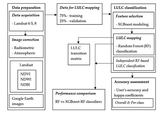
3.3. Comparative Assessment of RF and XGBoost- Feature Selected RF in LULC Classification

As noted above (see Section 2.4), to evaluate the performance of the XGBoost-RF classifier, a standalone RF classification was performed that yielded an average ~0.78 accuracy rate. Table 5 suggests this standalone RF classifier was outperformed by the XGBoost-feature selected RF classifier when classifying the LULC classes for every year. Table 7 shows (see also Figure A1 and Figure 4) the area of multi-temporal LULC classes obtained by RF and XGBoost-feature selected RF classifiers. LULC classifications performed by these two approaches differ quite significantly, particularly for agriculture, vegetation, and built-up area classes. Previous studies [3,12] focused on estimating LULC classes of small discrete regions in the coastal areas of Bangladesh, for which it is difficult to empirically validate these results. The RF-based estimations of multi-year LULC areas do not appear to reflect growing economic activity and documented large-scale natural disturbances (e.g., cyclones, storm surges) in Bangladesh’s coastal region over recent decades.

For instance, RF-based classification underestimated the obvious impacts of the natural processes and urbanization on coastal LULC distributions, particularly for agricultural land, bare soil, and built-up areas. The percentage area, estimated solely via RF-based classifications, often yielded values that were close to zero for the aforementioned classes. An example is the year 2010, where the RF-based classification in Table 7 shows a built-up area of only 0.04%, a percentage which contradicts the findings of several studies [3,12,47,61,62] that reported high rates of urbanization (hence an increased rate of development for built-up areas) in the past decade. Furthermore, the percentage area covered by the bare soil class was zero for the years 2005, 2010 and 2017, which for a hydrologically active area such as the coastal region of Bangladesh is quite impossible, especially because erosion and accretion processes (driven by the large river system) are highly prominent in this area [5,37,63]. In contrast, XGBoost-RF-derived results are more aligned with the growing human and natural activity trend across the whole coastal region. Comparison of RF only and the XGBoost-RF values for the percentage area covered by the built-up class indicates that the latter is consistent with the findings of previous studies. The XGBoost-RF-derived percentages agree with the increasing trend of the built-up class from 2005–2017, as could be expected due to a proliferation in the amount of urbanization during the last decade. Similarly, contrasting the percentage area covered by the bare soil class during 2005–2017, it is evident that the XGBoost-driven classification technique has performed better than the solely RF-driven classification process. For example, the percentage areas for bare class in the XGBoost-driven classified images were 7.90, 0.38 and 0.52 for the years 2005, 2010 and 2017 respectively; compared to a percentage of 0 in the RF only classified images. In addition, declining coastal vegetation coverage alongside increasing agricultural land areas, increasing amounts of bare soil areas following natural disturbances (e.g., floods in 1998 and 2004; and cyclones of 2007 and 2009), and the increasing amount of built-up area were picked up comparatively well by the XGBoost-RF classification approach.

As mentioned previously, several studies have reported that RF’s randomized bagging-based feature selection and classification approach can be biased towards the majority class and therefore, can misclassify the minority class in the data [18,19]. The findings from our study reiterate these shortcomings of the RF classifier, most notably when detecting minority classes (such as built-up land and bare soil) in a highly heterogeneous geomorphic setting.

3.4. Spatio-Temporal Patterns of LULC

Determining the spatio-temporal dynamics of LULC patterns in the coastal regions of Bangladesh requires a careful interpretation of the underlying natural and anthropogenic drivers that influence the pattern of LULC change. The coastal zone of Bangladesh is divided into western, eastern and central regions [64]; and each of these zones has its own characteristics and geomorphic processes that shape the LULC pattern. Because of the interplay between these natural processes and human activities, people living in these areas are constantly subjected to severe flooding, cyclones, and storm surges, which cause extensive destruction of property and force displacements within and outside the region. For example, the southwestern region relies predominantly on the upstream waters for land building activity and experiences a myriad of environmental issues such as high-level soil and river water salinity [65]. Similarly, the central zone is highly dynamic and various natural hazards such as storm surge-induced coastal flooding contribute to the environmental externalities. Although less frequent than the other two regions, the eastern zone is also affected by occasional cyclones and storm surges [3,66] and has undergone huge infrastructural development in the recent years. These natural processes, combined with the recent increase in anthropogenic activities such as construction of embankments to secure people and properties from coastal flooding, infrastructural development and the advancement of tourism sector are greatly influencing coastal dynamics [5,47,61,67]. Given the heavily intertwined human and natural processes within, for such a large and heterogeneous landscape, LULC classification using moderate resolution Landsat data is obviously a challenging task. As a result, and despite the use of powerful machine learning ensembles, some confusion in the detection and accurate classification of land covers is not surprising, especially when 10 out of the 19 coastal districts within the study area are susceptible to moderate to severe coastal flooding and cyclones [68,69,70,71].

The LULC transition matrix (

Table 8. Transition matrix showing the changes in percentage areas of the studied classes.

		Agriculture	Vegetation	Bare Soil	Built-up	Wetland	River
1990–1995	Agriculture	73.74	17.12	0.69	3.39	1.11	3.95
	Vegetation	41.98	49.05	0.44	2.61	1.15	4.77
	Bare soil	72.27	16.27	0.73	4.27	1.26	5.20
	Built-up	50.39	13.56	2.08	10.56	4.62	18.79
	Wetland	30.21	17.19	2.01	9.13	5.89	35.57
	River	4.08	2.90	0.70	1.54	2.59	88.19
1995–2000	Agriculture	74.81	16.32	3.64	2.63	1.52	1.08
	Vegetation	34.64	61.77	0.92	1.12	0.74	0.81
	Bare soil	45.70	5.43	23.93	3.07	11.81	10.06
	Built-up	54.04	12.88	10.45	7.12	9.33	6.18
	Wetland	39.01	10.10	5.69	3.20	24.45	17.55
	River	10.89	4.42	2.36	0.85	5.78	75.70
2000–2005	Agriculture	40.30	36.61	9.98	3.78	7.55	1.78
	Vegetation	18.55	71.18	4.05	1.33	3.96	0.93
	Bare soil	33.47	16.86	20.07	9.37	9.63	10.60
	Built-up	37.37	26.70	12.59	10.14	7.61	5.59
	Wetland	12.99	13.70	10.33	7.24	40.48	15.26
	River	3.01	3.62	5.43	1.94	8.82	77.18
2005–2010	Agriculture	57.72	30.41	0.39	6.91	1.83	2.74
	Vegetation	21.04	74.30	0.05	2.16	0.72	1.73
	Bare soil	57.60	19.39	1.55	10.48	3.93	7.05
	Built-up	52.41	16.54	0.40	15.09	7.25	8.31
	Wetland	39.98	10.87	0.27	7.20	22.75	18.93
	River	4.07	1.25	0.63	0.83	4.07	89.15
2010–2017	Agriculture	52.09	27.80	0.70	7.30	1.02	11.09
	Vegetation	11.78	82.16	0.10	3.06	0.28	2.62
	Bare soil	43.98	5.91	10.41	8.38	0.04	31.28
	Built-up	47.72	12.50	1.32	22.94	0.53	14.99
	Wetland	16.72	8.48	0.45	3.86	14.60	55.89
	River	3.38	2.54	0.75	1.31	0.99	91.03

), LULC maps (Figure 3), and a per-year distribution of LULC class sizes (in hectare) (Figure 4) demonstrate some interesting and important spatio-temporal patterns. It can be seen that the built-up areas experienced an increasing trend from 1990 to 2017, with a slight decrease in 2000 when a large proportion of human settlements on the southwestern coast was severely affected by the catastrophic flood of 2000 [72]. The effect of this flood was probably manifested in the degradation of vegetation for 2000, since a large proportion of coastal vegetation cover was probably washed away. It appears, however, that successful coastal afforestation initiatives [73] in successive years resulted in a gradual increase in vegetation, notably from 2000 to 2017 [73,74,75]. Flooding has also influenced the distribution of inland water bodies. The devastating flood event of 2004 caused massive waterlogging in the low-lying coastal areas due to drainage congestion and the associated backwater effect, resulting in a sharp increase in water bodies in the classified LULC map of 2005. The residual effect of this event was probably linked with the increased proportion of the wetland category in 2005. Although filling of (grabbing) water bodies including river areas is a common practice in a region where rapid urbanization is taking place over the past decades, an increasing pattern of river area since 2005 was observed in the coastal region. This phenomenon can be associated with the increased popularity and practice of shrimp cultivation, with possible links to factors such as sea-level rise and land subsidence, especially in the southwestern region [76,77,78]. Areas under agricultural activity showed an increasing trend between 1990 and 2000 with a decreasing trend in vegetation cover evident during the same period (Table 8).

A detailed analysis of the intra and inter-transition of LULC classes (Table 8) reveals that human-environment interactions are shaping the LULC dynamics of the coastal region. For example, contrary to common knowledge and perception, built-up areas in the coastal region of Bangladesh experienced conversion into other land cover types (e.g., agricultural land). This somewhat unconventional land use transition may be linked with coastal out-migration, induced predominantly by environmental disturbances and climate change [79,80]. Although it is not entirely clear as to how human migration could lead to land cover change, Braimoh (2004) demonstrated that seasonal migration resulted in dramatic land use change in Ghana [81]. Fasona and Omojola (2009), using remote sensing data, also noted that increased soil salinity via coastal erosion caused the loss of livelihoods, eventually leading to the dislocation of a total of 39 coastal communities in Nigeria [82]. In the case of the coastal area of Bangladesh, it is possible that migration may force people to sell their properties to local elites, and it is, in fact, the choice of the buyers as to whether to keep the newly purchased land in its present form or to convert it to other categories such as shrimp land for a higher economic return. However, this warrants further investigation.

In order to explore the transition of built-up class in detail, we examined the last two population censuses (2001 and 2011) of the coastal districts, and found that four districts located in the central and southwestern zones experienced negative population changes between 2001 and 2011 (

Table 9. Population change during 2001–2011 in the coastal areas of Bangladesh. Districts highlighted with bold face experienced a negative population change.

District Name	2001	2011	Population Change (%)
Bagerhat	1,549,031	1,476,090	−4.70881
Barguna	848,554	892,781	5.212043
Barisal	2,355,967	2,324,310	−1.34369
Bhola	1,703,117	1,776,795	4.326068
Chandpur	2,271,229	2,416,018	6.374919
Chittagong	6,612,140	7,616,352	15.1874
Cox’s Bazar	1,773,709	2,289,990	29.10742
Feni	1,240,384	1,437,371	15.88113
Gopalganj	1,165,273	1,172,415	0.612904
Jessore	2,471,554	2,764,547	11.85461
Jhalokati	694,231	682,669	−1.66544
Khulna	2,378,971	2,318,527	−2.54076
Lakshmipur	1,489,901	1,729,188	16.0606
Narail	698,447	721,668	3.324662
Noakhali	2,577,244	3,108,083	20.59716
Patuakhali	1,460,781	1,535,854	5.139237
Pirojpur	1,111,068	1,113,257	0.197018
Satkhira	1,864,704	1,985,959	6.502641
Shariatpur	1,082,300	1,155,824	6.793311

). A comparison of these population changes against yearly LULC maps in Figure 3 also supports the observation that the areas experiencing a disappearance of built-up pixels (when compared to the previous years) belong to these four districts, experiencing a decrease in population. This strongly suggests that depopulation resulting from natural hazards or anthropogenic causes may play a significant role in explaining the decline in built-up areas in 2000 and the low intra-class transition of pixels in Table 7 and Table 8, respectively. Furthermore, coastal erosion which is pervasive in many areas (particularly in the central zone), has, in the past, resulted in the loss of entire villages to the river or the sea. Given these observations, and the inconsistency in the built-up area/pixel transformation detailed, it is possible to suggest that the observations are indicative of the high-degree of human-environment interactions that govern LULC dynamics in Bangladesh’s coastal region.

However, it can also be observed that the conversion of built-up areas to other classes significantly declined after 2000 and now aligns more closely with the characteristics usually expected from this LULC class (remaining unchanged or showing an increased intra-class conversion). This could be the result of the various adaptation and disaster risk mitigation strategies implemented by the government and the non-government organizations in more recent times [69,83,84].

The spatio-temporal patterns of agricultural land cover show a gradual increase between 1990 and 2000; however, this trend has fluctuated in the period between 2000 and 2017. One particular aspect that may govern this fluctuation in post 2000 years could result from increasing shrimp farming activities. The spate of recurrent cyclones and flooding has impacted on the stability of crop production as a livelihood practice. Additionally, increasing soil salinity also made crop production increasingly difficult for the farmers [39,85]. Therefore, shrimp production, which is well suited to operating in the saline conditions and is less prone to environmental externalities, gained considerable prominence. The rising popularity of shrimp cultivation coupled with the natural calamities that took place during the study period (i.e., 1990–2017) can help understand the transition of agriculture to other classes in Table 8. Periodic waterlogging caused by embankment construction is another factor that could have shaped agricultural land cover. Embankments that were constructed in the 1960s to secure people and properties in the coastal region is a prime example of man-made activity that appears to interrupt the sedimentation process, hence the elevation loss of the land [86]. Consequently, water ingress into the areas behind the embankment walls during a cyclone or high tide events can lead to pervasive flooding of agricultural lands and human settlements [86]. It is evident that the percent area covered by the agricultural land remained almost unchanged during the 1990–1995 and 1995–2000 periods. However, a sharp decline was observed during 2000–2005 period, after which the change again became nearly constant in post-2005 periods. The recurrent floods and cyclones rendered most of the agricultural lands productively useless. The repeated displacements of people due to these natural disasters may have led to the abandonment of these agricultural lands, which were later colonized by different forms of vegetation cover (such as shrubs and bushes) and thus, accounting for the high transition between these two classes. Additionally, a total change, ranging from 9.33 to 12.11%, was found for the conversion of agricultural class to water bodies and river classes during the 2000–2017 period. Both the conversion of agricultural lands to shrimp farming and the formation of large temporary water bodies due to floods and cyclones can potentially account for this change. In such a dynamic situation, the recognition of pure pixels (even with an advanced ensemble) could be challenging as satellite data only represent a snapshot of a given time point.

The river and wetland classes in LULC maps show an alternating trend of increase and decrease between 1990 and 2017. In the LULC classification process, isolating wetlands and river areas, was difficult for the years when coastal flooding occurred (either by high tide/cyclone induced storm surges), when river water was used for irrigation purpose or used for shrimp cultivation. These factors appear to have played a crucial role in the classification process by mixing up inland water bodies and river areas [87,88]. Furthermore, after Cyclone Aila in 2009, numerous saline water bodies were created in the southwestern part of the region [89]. When inland water bodies reach a certain salinity threshold, the spectral reflectance of these inland water bodies becomes identical to that of the rivers [88,90,91,92,93]. Consequently, water bodies that are actually shrimp cultivation sites are classified as part of the river system. This aspect of spectral reflectance identification may be one of the reasons for the increasing trend of river areas being detected in the LULC maps of 2005, 2010 and 2017, as well as the high transition rate between water bodies and river classes in Table 8. Additionally, one of the popularly-practiced adaptation strategies for flood and waterlogging in the southern region can be identified in the LULC transition matrix in Table 8, that is—a large proportion of the water bodies seem to have converted into agricultural land. This may have resulted from alternating practice of shrimp cultivation and crop production in low-lying areas such as the beels [91,92]. Farmers resort to shrimp cultivation when these low elevation lands become inundated with water after intense rainstorms, and thus, for those years, the low-lying areas were classified as water bodies. In succeeding years, when there is not sufficient influx of water from the rainy season or the tide from the nearby rivers, these areas dry up and are again used for agricultural activities. As a result, large areas of land could have varied spectral responses when they are engulfed with rain or saline waters, or are used for agricultural purposes. This type of issue may be a common source of mixed pixels while employing moderate resolution images for LULC classification.

A significant decline in the amount of vegetation cover can be seen in LULC maps between 1990 and 2000. An intricate web of river systems and estuaries along the central zone makes it highly dynamic and susceptible to high-tide induced coastal floods [5], and this may result in the frequent submergence of built-up land and human settlements along with the removal of vegetation cover. Despite the eastern zone being relatively stable in terms of erosion and accretion processes [64], clearing of forest cover is pervasive, together with other increased human activities such as infrastructural development and urban expansion [94]. However, in the post 2000 years, areas with vegetation cover increased until 2017, which can be attributed to major coastal afforestation projects along the coastal belt undertaken since 2000 [73,74,75]. As a part of these projects, the Department of Forest from the government of Bangladesh took a mega initiative of planting 2872.88 hectares of Nipa, 10.0 hectares of coconut, 40.0 hectares of Arica palm, 280.0 hectares of Bamboo and Cane, 192,395.24 hectares of mangrove and 8689.53 hectares of non-mangrove trees. The effects of these afforestation projects are clearly visible in the LULC maps between 2005 and 2017. Table 8 further shows that a large portion of the vegetation cover in the study area remained unchanged during the study period (1990–2017) and that the intra-class percent conversion remained nearly above 50% from 1995–2017. This could be due mainly to the large mangrove forest occupying the southwestern region of the study area, which did not show any discernible change in the LULC maps (Figure 3a–f). Apart from this, vegetation plantations around homesteads are a popular measure used to save habitation and people from the ingress of frequent cyclones such as those that occurred in 2007 and 2009. This has become a common practice, to save communities against climate-influenced adversities, especially in the central coastal zone [95].

4. Conclusions

This study provided a detailed assessment of multi-temporal LULC changes in the coastal regions of Bangladesh using Landsat data and advanced feature selection and classification techniques—XGBoost and Random Forest. The XGBoost-based feature selection approach allowed detection of the most informative spectral bands. These contributed to the improved performance by the RF classifier in producing six-class LULC maps. This joint XGBoost-RF approach performed substantially better than an independent RF classifier when dealing with high-level landscape heterogeneity and spectral complexity issues (e.g., dominance of mixed pixels/LULC areas) in 30-m Landsat images during the LULC classification process. This improvement is indicated by the user’s accuracy and Kappa coefficient values of 0.80 and 0.75, respectively. The spatio-temporal investigation of the classified LULC maps shows that over the past 28 years (1990–2017) the coastal regions of Bangladesh have experienced an increase in agricultural land (5.44%), and in both built-up (4.91%) and river (4.52%) areas. The vegetation coverage across coastal landscapes experienced a significant decline in some years due to large-scale natural disturbances (e.g., flooding, cyclones and storm surges in 1996, 1997, 1998, 2004 and 2007) as well as human-influenced alterations (e.g., shrimp farming). However, the 2005–2017 LULC maps show a substantial overall increase in areas corresponding to the vegetation class—an understandable manifestation of the effect of coastal reforestation projects undertaken by the governmental and non-governmental entities in Bangladesh. These findings on the spatio-temporal dynamics of LULC can inform policy guidelines that are essential for combating the adverse effects of human-caused and natural disturbances across the entire coastal regions of Bangladesh.

This study also demonstrated that the use of powerful ensemble techniques such as XGBoost and Random Forest can be useful in addressing the complexities inherent in the LULC classification of a large and heterogeneous geographic area, particularly when available remotely sensed data come with insufficient spatial and spectral resolution. An effective collaboration among these techniques offers an excellent opportunity for frequent and detailed monitoring of the space-time LULC patterns of a rapidly changing landscape, especially in developing regions of the Asian subcontinent, which often rely on freely available lower-quality remotely sensed data. However, the results from this study should be interpreted with caution, since it is very challenging even for advanced algorithms to deal effectively with discriminating class memberships of a very large and complex landscapes by using lower to moderate spatial/spectral resolution imageries (i.e., Landsat). In fact, this large-scale study provides a useful methodological direction that should be further explored by future studies, using available remotely sensed data of varied qualities.

References

1. Camilleri, S.; De Giglio, M.; Stecchi, F.; Pérez-Hurtado, A. Land use and land cover change analysis in predominantly man-made coastal wetlands: Towards a methodological framework. Wetl. Ecol. Manag. 2017, 25, 23–43. [Google Scholar] [CrossRef]
2. Minar, M.; Hossain, B.; Shamsuddin, M. Climate change and coastal zone of Bangladesh: Vulnerability, resilience and adaptability. Middle-East J. Sci. Res. 2013, 13, 114–120. [Google Scholar]
3. Islam, M.R.; Miah, M.G.; Inoue, Y. Analysis of land use and land cover changes in the coastal area of Bangladesh using landsat imagery. Land Degrad. Dev. 2016, 27, 899–909. [Google Scholar] [CrossRef]
4. Mukhopadhyay, A.; Hornby, D.D.; Hutton, C.W.; Lázár, A.N.; Johnson, F.A.; Ghosh, T. Land Cover and Land Use Analysis in Coastal Bangladesh. In Ecosystem Services for Well-Being in Deltas; Palgrave Macmillan: Cham, Switzerland, 2018; pp. 367–381. [Google Scholar]
5. Brammer, H. Bangladesh’s dynamic coastal regions and sea-level rise. Clim. Risk. Manag. 2014, 1, 51–62. [Google Scholar] [CrossRef]
6. Otukei, J.R.; Blaschke, T. Land cover change assessment using decision trees, support vector machines and maximum likelihood classification algorithms. Int. J. Appl. Earth Obs. Geoinf. 2010, 12, S27–S31. [Google Scholar] [CrossRef]
7. Aplin, P. Comparison of simulated IKONOS and SPOT HRV imagery for classifying urban areas. In Remote Sensed Cities; Mesev, V., Ed.; CRC Press: London, UK; New York, NY, USA, 2003; pp. 23–45. [Google Scholar]
8. Rodriguez-Galiano, V.; Chica-Olmo, M.; Abarca-Hernandez, F.; Atkinson, P.M.; Jeganathan, C. Random Forest classification of Mediterranean land cover using multi-seasonal imagery and multi-seasonal texture. Remote Sens. Environ. 2012, 121, 93–107. [Google Scholar] [CrossRef]
9. Rodriguez-Galiano, V.F.; Ghimire, B.; Rogan, J.; Chica-Olmo, M.; Rigol-Sanchez, J.P. An assessment of the effectiveness of a random forest classifier for land-cover classification. Isprs Int. J. Geoinf. 2012, 67, 93–104. [Google Scholar] [CrossRef]
10. Lu, D.; Weng, Q. A survey of image classification methods and techniques for improving classification performance. Int. J. Remote Sens. 2007, 28, 823–870. [Google Scholar] [CrossRef]
11. Adam, E.; Mutanga, O.; Odindi, J.; Abdel-Rahman, E.M. Land-use/cover classification in a heterogeneous coastal landscape using RapidEye imagery: Evaluating the performance of random forest and support vector machines classifiers. Int. J. Remote Sens. 2014, 35, 3440–3458. [Google Scholar] [CrossRef]
12. Rahman, M.T.U.; Tabassum, F.; Rasheduzzaman, M.; Saba, H.; Sarkar, L.; Ferdous, J.; Uddin, S.Z.; Islam, A.Z. Temporal dynamics of land use/land cover change and its prediction using CA-ANN model for southwestern coastal Bangladesh. Envrion. Monit. Assess. 2017, 189, 565. [Google Scholar] [CrossRef] [PubMed]
13. Belgiu, M.; Drăguţ, L. Random forest in remote sensing: A review of applications and future directions. Isprs Int. J. Geoinf. 2016, 114, 24–31. [Google Scholar] [CrossRef]
14. Mountrakis, G.; Im, J.; Ogole, C. Support vector machines in remote sensing: A review. Isprs Int. J. Geoinf. 2011, 66, 247–259. [Google Scholar] [CrossRef]
15. Breiman, L. Random forests. Mach. Learn. 2001, 45, 5–32. [Google Scholar] [CrossRef]
16. DeFries, R.; Townshend, J. NDVI-derived land cover classifications at a global scale. Int. J. Remote Sens. 1994, 15, 3567–3586. [Google Scholar] [CrossRef]
17. Gislason, P.O.; Benediktsson, J.A.; Sveinsson, J.R. Random forests for land cover classification. Pattern Recognit. Lett. 2006, 27, 294–300. [Google Scholar] [CrossRef]
18. Puissant, A.; Rougier, S.; Stumpf, A. Object-oriented mapping of urban trees using Random Forest classifiers. Int. J. Appl. Earth Obs. Geoinf. 2014, 26, 235–245. [Google Scholar] [CrossRef]
19. He, H.; Garcia, E.A. Learning from imbalanced data. IEEE Trans. Knowl. Data Eng. 2008, 21, 1263–1284. [Google Scholar]
20. Strobl, C.; Boulesteix, A.-L.; Kneib, T.; Augustin, T.; Zeileis, A. Conditional variable importance for random forests. BMC Bioinform. 2008, 9, 307. [Google Scholar] [CrossRef]
21. Zhang, Y.; Mishra, R.K. A review and comparison of commercially available pan-sharpening techniques for high resolution satellite image fusion. In Proceedings of the 2012 IEEE International Geoscience and Remote Sensing Symposium, Munich, Germany, 22–27 July 2012; pp. 182–185. [Google Scholar]
22. Gilbertson, J.K.; Van Niekerk, A. Value of dimensionality reduction for crop differentiation with multi-temporal imagery and machine learning. Comput. Electron. Agric. 2017, 142, 50–58. [Google Scholar] [CrossRef]
23. Tibshirani, R. Regression shrinkage and selection via the lasso. J. R. Stat. Soc. Ser. B. Stat. Methodol. 1996, 58, 267–288. [Google Scholar] [CrossRef]
24. Conrad, C.; Colditz, R.; Dech, S.; Klein, D.; Vlek, P. Improved irrigated crop classification in Central Asia using temporal segmentation and MODIS time series. Int. J. Remote Sens. 2011, 32, 8763–8778. [Google Scholar] [CrossRef]
25. Yu, Q.; Gong, P.; Clinton, N.; Biging, G.; Kelly, M.; Schirokauer, D. Object-based detailed vegetation classification with airborne high spatial resolution remote sensing imagery. Photogramm. Eng. Remote Sens. 2006, 72, 799–811. [Google Scholar] [CrossRef]
26. Hao, P.; Wang, L.; Zhan, Y.; Niu, Z.; Wu, M. Using historical NDVI time series to classify crops at 30m spatial resolution: A case in Southeast Kansas. In Proceedings of the 2016 IEEE International Geoscience and Remote Sensing Symposium (IGARSS), Beijing, China, 10–15 July 2016; pp. 6316–6319. [Google Scholar]
27. Kim, H.; Loh, W.-Y. Classification trees with unbiased multiway splits. J. Am. Stat. Assoc. 2001, 96, 589–604. [Google Scholar] [CrossRef]
28. White, A.P.; Liu, W.Z. Bias in information-based measures in decision tree induction. Mach. Learn. 1994, 15, 321–329. [Google Scholar] [CrossRef]
29. Cui, B.; Zhang, N.; Xu, J.; Lian, X.; Liu, D. Web-Age Information Management; Springer: Berlin, Germany, 2016. [Google Scholar]
30. Zheng, H.; Yuan, J.; Chen, L. Short-term load forecasting using EMD-LSTM neural networks with a Xgboost algorithm for feature importance evaluation. Energies 2017, 10, 1168. [Google Scholar] [CrossRef]
31. Sheridan, R.P.; Wang, W.M.; Liaw, A.; Ma, J.; Gifford, E.M. Extreme gradient boosting as a method for quantitative structure–activity relationships. J. Chem. Inf. Model 2016, 56, 2353–2360. [Google Scholar] [CrossRef] [PubMed]
32. Georganos, S.; Grippa, T.; Vanhuysse, S.; Lennert, M.; Shimoni, M.; Kalogirou, S.; Wolff, E. Less is more: Optimizing classification performance through feature selection in a very-high-resolution remote sensing object-based urban application. Gisci. Remote Sens. 2018, 55, 221–242. [Google Scholar] [CrossRef]
33. Jiang, S.; Zhao, H.; Wu, W.; Tan, Q. A novel framework for remote sensing image scene classification. Int. Arch. Photogram. Remote Sens. Spat. Inf. Sci. 2018, 42, 657–663. [Google Scholar] [CrossRef]
34. Rao, H.; Shi, X.; Rodrigue, A.K.; Feng, J.; Xia, Y.; Elhoseny, M.; Yuan, X.; Gu, L. Feature selection based on artificial bee colony and gradient boosting decision tree. Appl. Soft Comput. 2019, 74, 634–642. [Google Scholar] [CrossRef]
35. Zhong, L.; Hu, L.; Zhou, H. Deep learning based multi-temporal crop classification. Remote Sens. Environ. 2019, 221, 430–443. [Google Scholar] [CrossRef]
36. Khan, M.M.H.; Bryceson, I.; Kolivras, K.N.; Faruque, F.; Rahman, M.M.; Haque, U. Natural disasters and land-use/land-cover change in the southwest coastal areas of Bangladesh. Reg. Environ. Chang. 2015, 15, 241–250. [Google Scholar] [CrossRef]
37. Brammer, H. Physical Geography of Bangladesh; The University Press Ltd.: Hong Kong, China, 2012. [Google Scholar]
38. Islam, M.R.; Abdullah, H.M.; Ahmed, Z.U.; Islam, I.; Ferdush, J.; Miah, M.G.; Miah, M.M.U. Monitoring the spatiotemporal dynamics of waterlogged area in southwestern Bangladesh using time series Landsat imagery. Remote Sens. Appl. Soc. Environ. 2018, 9, 52–59. [Google Scholar] [CrossRef]
39. Abdullah, A.Y.M.; Biswas, R.K.; Chowdhury, A.I.; Billah, S.M. Modeling soil salinity using direct and indirect measurement techniques: A comparative analysis. Environ. Dev. 2018, 29, 67–80. [Google Scholar] [CrossRef]
40. Bricheno, L.; Wolf, J. Modelling Tidal River Salinity in Coastal Bangladesh. In Ecosystem Services for Well-Being in Deltas: Integrated Assessment for Policy Analysis; Springer: Cham, Switzerland, 2018; p. 315. [Google Scholar]
41. Aziz, A.; Paul, A.R. Bangladesh Sundarbans: Present status of the environment and biota. Diversity 2015, 7, 242–269. [Google Scholar] [CrossRef]
42. Islam, S.N.; Reinstädtler, S.; Gnauck, A. Vulnerability of Mangrove Forests and Wetland Ecosystems in the Sundarbans Natural World Heritage Site (Bangladesh). In Threats to Mangrove Forests; Springer: Cham, Switzerland, 2018; pp. 223–243. [Google Scholar]
43. Giri, C.; Pengra, B.; Zhu, Z.; Singh, A.; Tieszen, L.L. Monitoring mangrove forest dynamics of the Sundarbans in Bangladesh and India using multi-temporal satellite data from 1973 to 2000. Estuar. Coast Shelf Sci. 2007, 73, 91–100. [Google Scholar] [CrossRef]
44. Emch, M.; Peterson, M. Mangrove forest cover change in the Bangladesh Sundarbans from 1989–2000: A remote sensing approach. Geocarto Int. 2006, 21, 5–12. [Google Scholar] [CrossRef]
45. Bangladesh Meteorological Department. Available online: http://www.bmd.gov.bd/ (accessed on 3 February 2018).
46. Parvin, G.A.; Ali, M.H.; Fujita, K.; Abedin, M.A.; Habiba, U.; Shaw, R. Land use change in southwestern coastal Bangladesh: Consequence to food and water supply. In Land Use Management in Disaster Risk Reduction; Springer: Cham, Switzerland, 2017; pp. 381–401. [Google Scholar]
47. Mia, M.A.; Nasrin, S.; Zhang, M.; Rasiah, R. Chittagong, Bangladesh. Cities 2015, 48, 31–41. [Google Scholar] [CrossRef]
48. Kashem, M.A.; Siddiqui, A.A.M.; Mahbubur, M. Coastal zone of Khulna district in Bangladesh: Fisheries land use and its potentials. Int. J. Fish. Aquat. Stud. 2017, 5, 599–608. [Google Scholar]
49. USGS. Landsat 8 Data Users Handbook—Section 5. 2017. Available online: https://www.usgs.gov/land-resources/nli/landsat (accessed on 3 February 2018).
50. Song, C.; Woodcock, C.E.; Seto, K.C.; Lenney, M.P.; Macomber, S.A. Classification and change detection using Landsat TM data: When and how to correct atmospheric effects? Remote Sens. Environ. 2001, 75, 230–244. [Google Scholar] [CrossRef]
51. Lawrence, R.; Bunn, A.; Powell, S.; Zambon, M. Classification of remotely sensed imagery using stochastic gradient boosting as a refinement of classification tree analysis. Remote Sens. Envrion. 2004, 90, 331–336. [Google Scholar] [CrossRef]
52. Just, A.C.; De Carli, M.M.; Shtein, A.; Dorman, M.; Lyapustin, A.; Kloog, I. Correcting Measurement Error in Satellite Aerosol Optical Depth with Machine Learning for Modeling PM2.5 in the Northeastern USA. Remote Sens. 2018, 10, 803. [Google Scholar] [CrossRef]
53. Freeman, E.A.; Moisen, G.G.; Coulston, J.W.; Wilson, B.T. Random forests and stochastic gradient boosting for predicting tree canopy cover: Comparing tuning processes and model performance. Can. J. Res. 2015, 46, 323–339. [Google Scholar] [CrossRef]
54. Man, C.D.; Nguyen, T.T.; Bui, H.Q.; Lasko, K.; Nguyen, T.N.T. Improvement of land-cover classification over frequently cloud-covered areas using Landsat 8 time-series composites and an ensemble of supervised classifiers. Int. J. Remote Sens. 2018, 39, 1243–1255. [Google Scholar] [CrossRef]
55. Bradley, A.P. The use of the area under the ROC curve in the evaluation of machine learning algorithms. Pattern Recognit. 1997, 30, 1145–1159. [Google Scholar] [CrossRef]
56. Fan, J.; Upadhye, S.; Worster, A. Understanding receiver operating characteristic (ROC) curves. CJEM 2006, 8, 19–20. [Google Scholar] [CrossRef] [PubMed]
57. Southworth, J. An assessment of Landsat TM band 6 thermal data for analysing land cover in tropical dry forest regions. Int. J. Remote Sens. 2004, 25, 689–706. [Google Scholar] [CrossRef]
58. Sun, L.; Schulz, K. The improvement of land cover classification by thermal remote sensing. Remote Sens. 2015, 7, 8368–8390. [Google Scholar] [CrossRef]
59. Toloşi, L.; Lengauer, T. Classification with correlated features: Unreliability of feature ranking and solutions. Bioinformatics 2011, 27, 1986–1994. [Google Scholar] [CrossRef]
60. Abdullah, A.Y.M.; Dewan, A.; Shogib, M.R.I.; Rahman, M.M.; Hossain, M.F. Environmental factors associated with the distribution of visceral leishmaniasis in endemic areas of Bangladesh: Modeling the ecological niche. Trop. Med. Health 2017, 45, 13. [Google Scholar] [CrossRef]
61. Hossain, M.S.; Lin, C.K.; Tokunaga, M.; Demaine, H.; Hussain, M.Z. Land Use Zoning for Salt Production in Cox’s Bazar Coast of Bangladesh: A Remote Sensing and GIS Analysis. Asian J. Geoinform. 2003, 3, 69–77. [Google Scholar]
62. Ahmed, B.; Dewan, A. Application of bivariate and multivariate statistical techniques in landslide susceptibility modeling in Chittagong city corporation, Bangladesh. Remote Sens. 2017, 9, 304. [Google Scholar] [CrossRef]
63. Brammer, H. Geographical complexities of detailed impact assessment for the Ganges-Brahmaputra-Meghna delta of Bangladesh. In Climate and Sea Level Change: Observations, Projections and Implications; Cambridge University Press: Cambridge, UK, 1993; pp. 246–262. [Google Scholar]
64. Sarwar, M.G.M.; Woodroffe, C.D. Rates of shoreline change along the coast of Bangladesh. J. Coast. Conserv. 2013, 17, 515–526. [Google Scholar] [CrossRef]
65. Akter, J.; Sarker, M.H.; Popescu, I.; Roelvink, D. Evolution of the Bengal Delta and its prevailing processes. J. Coast. Res. 2015, 32, 1212–1226. [Google Scholar] [CrossRef]
66. Chiu, S.; Small, C. Observations of cyclone-induced storm surge in coastal Bangladesh. J. Coast. Res. 2016, 32, 1149–1161. [Google Scholar] [CrossRef]
67. Pethick, J.; Orford, J.D. Rapid rise in effective sea-level in southwest Bangladesh: Its causes and contemporary rates. Glob. Planet. Chang. 2013, 111, 237–245. [Google Scholar] [CrossRef]
68. Chowdhury, A.M.R.; Bhuyia, A.U.; Choudhury, A.Y.; Sen, R. The Bangladesh cyclone of 1991: Why so many people died. Disasters 1993, 17, 291–304. [Google Scholar] [CrossRef]
69. Paul, B.K. Why relatively fewer people died? The case of Bangladesh’s Cyclone Sidr. Nat. Hazards 2009, 50, 289–304. [Google Scholar] [CrossRef]
70. Dasgupta, S.; Hossain, M.; Huq, M.; Wheeler, D. Climate change, Soil Salinity, and the Economics of High-Yield Rice Production in Coastal Bangladesh; Policy Research Working Papers; International Bank for Reconstruction and Development: Washington, DC, USA, 2014. [Google Scholar] [CrossRef]
71. Dastagir, M.R. Modeling recent climate change induced extreme events in Bangladesh: A review. Weather Clim. Extrem. 2015, 7, 49–60. [Google Scholar] [CrossRef]
72. Ahmed, S. Setting the Stage. In Moving Coastlines; de Wilde, K., Ed.; The University Press Limited: Dhaka, Bangladesh, 2011. [Google Scholar]
73. Hassan, D.Z. Coastal Afforestation in Bangladesh and Its Role. Available online: http://www.theguardianbd.com/coastal-afforestation-in-bangladesh-and-its-role/ (accessed on 24 December 2018).
74. UNDP. Community based Adaptation to Climate Change through Coastal Afforestation in Bangladesh. Available online: https://adaptation-undp.org/projects/ldcf-cba-bangladesh (accessed on 24 December 2018).
75. Hossain, M.S.; Lin, C.K.; Hussain, M.Z. Remote sensing and GIS applications for suitable mangrove afforestation area selection in the coastal zone of Bangladesh. Geocarto Int. 2003, 18, 61–65. [Google Scholar] [CrossRef]
76. Paul, B.G.; Vogl, C.R. Impacts of shrimp farming in Bangladesh: Challenges and alternatives. Ocean Coast. Manag. 2011, 54, 201–211. [Google Scholar] [CrossRef]
77. Ali, A.M.S. Rice to shrimp: Land use/land cover changes and soil degradation in Southwestern Bangladesh. Land Use Policy 2006, 23, 421–435. [Google Scholar] [CrossRef]
78. Brown, S.; Nicholls, R. Subsidence and human influences in mega deltas: The case of the Ganges–Brahmaputra–Meghna. Sci. Total Envion. 2015, 527, 362–374. [Google Scholar] [CrossRef]
79. Chen, J.; Mueller, V. Coastal climate change, soil salinity and human migration in Bangladesh. Nat. Clim. Chang. 2018, 8, 981. [Google Scholar] [CrossRef]
80. Martin, M.; Kang, Y.H.; Billah, M.; Siddiqui, T.; Black, R.; Kniveton, D. Climate-influenced migration in Bangladesh: The need for a policy realignment. Dev. Policy Rev. 2017, 35, O357–O379. [Google Scholar] [CrossRef]
81. Braimoh, A. Seasonal migration and land-use change in Ghana. Land Degrad. Dev. 2004, 15, 37–47. [Google Scholar] [CrossRef]
82. Fasona, M.; Omojola, A. Land cover change and land degradation in parts of the southwest coast of Nigeria. Afr. J. Ecol. 2009, 47, 30–38. [Google Scholar] [CrossRef]
83. Hashizume, M.; Dewan, A.M.; Sunahara, T.; Rahman, M.Z.; Yamamoto, T. Hydroclimatological variability and dengue transmission in Dhaka, Bangladesh: A time-series study. BMC Infect. Dis. 2012, 12, 98. [Google Scholar] [CrossRef] [PubMed]
84. Dasgupta, S.; Huq, M.; Khan, Z.H.; Ahmed, M.M.Z.; Mukherjee, N.; Khan, M.F.; Pandey, K. Cyclones in a changing climate: The case of Bangladesh. Clim. Dev. 2014, 6, 96–110. [Google Scholar] [CrossRef]
85. Haque, S. Salinity problems and crop production in coastal regions of Bangladesh. Pak. J. Bot. 2006, 38, 1359–1365. [Google Scholar]
86. Auerbach, L.; Goodbred, S., Jr.; Mondal, D.; Wilson, C.; Ahmed, K.; Roy, K.; Steckler, M.; Small, C.; Gilligan, J.; Ackerly, B. Flood risk of natural and embanked landscapes on the Ganges–Brahmaputra tidal delta plain. Nat. Clim. Chang. 2015, 5, 153. [Google Scholar] [CrossRef]
87. Jensen, J.R. Introductory Digital Image Processing: A Remote Sensing Perspective; University of South Carolina, Columbus: Columbia, SC, USA, 1986. [Google Scholar]
88. Jensen, J.R. Remote Sensing of the Environment: An Earth Resource Perspective, 2nd ed.; Pearson Education India: New Delhi, India, 2009. [Google Scholar]
89. Mallick, B.; Rahaman, K.R.; Vogt, J. Coastal livelihood and physical infrastructure in Bangladesh after cyclone Aila. Mitig. Adapt. Strat. Glob. Chang. 2011, 16, 629–648. [Google Scholar] [CrossRef]
90. Clarke, D.; Williams, S.; Jahiruddin, M.; Parks, K.; Salehin, M. Projections of on-farm salinity in coastal Bangladesh. Environ. Sci. Process Impacts 2015, 17, 1127–1136. [Google Scholar] [CrossRef] [PubMed]
91. Ding, J.; Yu, D. Monitoring and evaluating spatial variability of soil salinity in dry and wet seasons in the Werigan–Kuqa Oasis, China, using remote sensing and electromagnetic induction instruments. Geoderma 2014, 235, 316–322. [Google Scholar] [CrossRef]
92. Dwivedi, R. Study of salinity and waterlogging in Uttar Pradesh (India) using remote sensing data. Land Degrad. Dev. 1994, 5, 191–199. [Google Scholar] [CrossRef]
93. Michot, B.; Meselhe, E.; Krauss, K.W.; Shrestha, S.; From, A.S.; Patino, E. Hydrologic modeling in a marsh–mangrove ecotone: Predicting wetland surface water and salinity response to restoration in the Ten Thousand Islands region of Florida, USA. J. Hydrol. Eng. 2015, 22, D4015002. [Google Scholar] [CrossRef]
94. Rahman, S.; Rahman, M.A. Climate extremes and challenges to infrastructure development in coastal cities in Bangladesh. Weather Clim. Extrem. 2015, 7, 96–108. [Google Scholar] [CrossRef]
95. Rawlani, A.K.; Sovacool, B.K. Building responsiveness to climate change through community based adaptation in Bangladesh. Mitig. Adapt. Strat. Glob. Chang. 2011, 16, 845–863. [Google Scholar] [CrossRef]
Figure 1. Location of the study area showing the coastal districts of Bangladesh.
Remotesensing 11 00790 g001
Figure 2. Flowchart showing overall methodology of this work.
Remotesensing 11 00790 g002
Figure 3. Classified land cover maps of the coastal area of Bangladesh: (a) 1990, (b) 1995, (c) 2000, (d) 2005, (e) 2010 and (f) 2017.
Remotesensing 11 00790 g003aRemotesensing 11 00790 g003bRemotesensing 11 00790 g003c
Figure 4. Percent area distribution of each land cover class between 1990 and 2017, obtained by the XGBoost-RF classifier.
Remotesensing 11 00790 g004