IMU/Magnetometer/Barometer/Mass-Flow Sensor Integrated Indoor Quadrotor UAV Localization with Robust Velocity Updates

Abstract

Velocity updates have been proven to be important for constraining motion-sensor-based dead-reckoning (DR) solutions in indoor unmanned aerial vehicle (UAV) applications. The forward velocity from a mass flow sensor and the lateral and vertical non-holonomic constraints (NHC) can be utilized for three-dimensional (3D) velocity updates. However, it is observed that (a) the quadrotor UAV may have a vertical velocity trend when it is controlled to move horizontally; (b) the quadrotor may have a pitch angle when moving horizontally; and (c) the mass flow sensor may suffer from sensor errors, especially the scale factor error. Such phenomenons degrade the performance of velocity updates. Thus, this paper presents a multi-sensor integrated localization system that has more effective sensor interactions. Specifically, (a) the barometer data are utilized to detect height changes and thus determine the weight of vertical velocity update; (b) the pitch angle from the inertial measurement unit (IMU) and magnetometer data fusion is used to set the weight of forward velocity update; and (c) an extra mass flow sensor calibration module is introduced. Indoor flight tests have indicated the effectiveness of the proposed sensor interaction strategies in enhancing indoor quadrotor DR solutions, which can also be used for detecting outliers in external localization technologies such as ultrasonics.

1. Introduction

Unmanned aerial vehicles (UAV) have shown great potential in civilian applications such as indoor/outdoor mapping [1], target tracking [2], victim searching [3], and industrial inspection [4]. For these applications, a key is the real-time estimation of UAV navigation states (i.e., position, velocity, and attitude). Although the integration of data from global navigation satellite systems (GNSS), real-time kinematics (RTK), or precise point positioning (PPP) and inertial measurement units (IMU) have been successfully commercialized to provide accurate (i.e., decimeter and centimeter level location accuracy for dynamic and static applications, respectively) location solutions in outdoor areas [5], reliable indoor UAV localization is a challenge due to the degradation of GNSS signals.

To alleviate this issue, researchers have presented various systems and approaches.

Table 1. Selected systems and methods for indoor unmanned aerial vehicles (UAV) localization from the years 2016 to 2018.

Method	Sensors	Algorithm	Test Area	Accuracy
[6]	Stereo camera	SLAM	200 m * 300 m	Meter level
[7]	Stereo camera, IMU	SLAM	16 m * 16 m	Meter level
[8]	Monocular camera, IMU	Kernel adaptive filtering	N/A	Decimeter level
[9]	Monocular camera, optical flow sensor, IMU, barometer	Indirect EKF	50 m * 20 m	Meter level
[10]	Monocular camera, fiducial markers	Relative pose identification	5 m * 5 m	Decimeter level
[11]	RGB-D camera, IMU, ultrasonic, optical flow sensor	Decentralized information filter	3 m * 2 m	Decimeter level
[12]	Optical flow sensor, IMU	EKF	6 m * 6 m	0.3 m in mean
[13]	Ultraviolet LED makers	Mutual relative localization	10 m distance	Meter level
[14]	3D lidar, UWB, IMU	EKF	Simulation	Decimeter level
[15]	2D lidar	CNN	4 m * 4 m	Decimeter level
[16]	2D lidar, IMU	SLAM	8 m * 8 m	1.0 m for 26 s, 0.5 m for 10 s
[17]	2D lidar, IMU	Tightly coupled SLAM	60 m corridor	Meter level
[18]	1D laser, IMU, barometer	EKF	5 m * 9 m	0.1 m height accuracy in mean
[19]	Radar	Radar odometry	80 m * 10 m	3.3 m in mean
[20]	Radar, UWB, IMU	EKF	40 m * 40 m	0.8 m in RMS
[21]	UWB	Multilateration	20 m * 30 m, 4 AP	2.0 m in mean
[22]	UWB	TDoA	4 m * 2 m, 4 AP	0.1 m in 75 %
[23]	UWB, IMU	Tightly coupled EKF	19 m * 13 m	0.15 m in mean
[24]	UWB, monocular camera	SLAM	8 m * 8 m	0.23 m in 75 %
[25]	UWB, RGB-D camera	Monte Carlo localization	15 m * 15 m	0.2 m in RMS
[26]	Ultrasonic	Multilateration	4 m * 3 m, 6 AP	0.16 m in RMS
[27]	Ultrasonic	CNN	10 m * 4 m	Decimeter level
[28]	Ultrasonic, time-of-flight camera	Multilateration	0.7 m * 0.7 m, 5 AP	0.17 m in median
[29]	WiFi	Fingerprinting	36 m * 17 m, 10 APs	1.7 m in mean
[30]	WiFi	Fingerprinting with RSS interpolation	9 m * 9 m, 4 APs	2.2 m in mean
[31]	BLE	Multilateration	4 m * 4 m	Meter level
[32]	RFID, GNSS (RTK)	K-nearest neighbors	30 m * 30 m, 9 tags	0.18 m in RMS
[33]	Magnetometers	Magnetic matching	24 m * 2 m	Sub-meter level
[34]	Hall-effect sensor, IMU	EKF	30 m * 30 m	2.15 m in 54 s
[35]	A quasi-taut tether	Angle and range-based	2.5 m * 2.5 m	0.37 m in mean

* SLAM—simultaneous localization and mapping; 1D/2D/3D—one/two/three-dimensional; EKF—extended Kalman filter; PF—particle filter; CNN—convolution neural network; RGB-D—red-green-blue-depth; RMS—root mean squares; TDoA—time-difference-of-arrival; RFID—radio frequency identification; LED—light-emitting diode; RSS—received signal strength; AP—access point; WiFi—wireless fidelity; BLE—Bluetooth low energy; N/A—not provided.

lists part of the existing works from the years 2016 to 2018. The used sensors and algorithms are shown as well as their test areas and location accuracies.

From the existing indoor localization works, the following phenomenons can be found:

• The candidate sensors include vision sensors (e.g., camera, lidar, and optical flow sensor), motion sensors (e.g., IMU, mass flow sensor, and the Hall-effect sensor), wireless sensors (e.g., UWB, ultrasonic, radar, WiFi, Bluetooth low energy (BLE), and radio frequency identification (RFID)), and environmental sensors (e.g., magnetometer and barometer).
• Different types of sensors typically provide various localization accuracies and meanwhile have different costs and coverage areas. Thus, there is a trade-off between performance and cost/coverage.
• High-precision wireless technologies (e.g., UWB and ultrasonic) can provide high localization accuracy (e.g., decimeter or even centimeter level). However, although the prices for low-cost commercial UWB and ultrasonic development kits have been reduced to the hundreds of dollars level, such systems have limited ranges (e.g., 30 m between nodes and anchors). Thus, other technologies are required to bridge their signal outages in wide-area applications. Meanwhile, for wireless ranging systems, there are inherent issues such as signal obstruction and multipath [36]. Thus, other technologies are needed to ensure localization reliability and integrity.
• Cameras and lidars can also provide high location accuracy when loop closures are correctly detected. Furthermore, some previous issues, such as heavy computational load, are being eliminated because of the development of modern processors and wireless data transmission technologies. However, the performance of vision-based localization systems is highly dependent on whether the measured features are distinct in space and stable over time. For database matching, any inconsistency between the measured data and the database may cause mismatches [37]. For mobile mapping, it is possible to add updates and loop closures to control errors. However, real-world localization conditions are complex and unpredictable; thus, it is difficult to maintain accuracy in challenging environments (e.g., areas with glass or solid-color walls). Therefore, external technologies may be needed to bridge such task periods as well as detect the outliers in vision sensor measurements.
• Dead-reckoning (DR) solutions from IMUs have been widely used to bridge other localization technologies’ signal outages and integrate with them to provide smoother and more robust solutions [38]. However, traditional navigation- or tactical-grade IMUs are heavy and costly and thus are not suitable for consumer-level UAVs. Micro-electro-mechanical systems (MEMS) IMUs are light and low-cost, which have made them suitable for low-cost indoor localization. However, low-cost MEMS IMUs suffer from significant run-to-run biases and thermal drifts [39], which are issues inherent to MEMS sensors. Therefore, standalone IMU-based DR solutions will drift over time. Magnetometer measurements can be used to derive an absolute heading update. However, the indoor magnetic declination angle becomes unknown, which makes the magnetometer heading unreliable [40]. Thus, it is still important to implement periodical updates to correct DR solutions.
• Vehicle motion model updates can be used to enhance the navigation system observability [41], especially when there are significant vehicle dynamics (e.g., accelerating or turning). Sensors such as the mass flow and Hall-effect sensors can measure the forward velocity. Meanwhile, it is assumed that the lateral and vertical velocity components are zeroes plus noises when the UAV is being controlled to move horizontally, i.e., the non-holonomic constraint (NHC) [42]. Accordingly, 3D velocity updates can be applied. Furthermore, there are other updates, such as the zero velocity update (ZUPT) and zero angular rate update (ZARU) when the UAV is hovering in a quasi-static mode [43]. These updates are effective when the actual UAV motion meets the assumption. However, in contrast to land vehicles that are constrained by the road surface, UAVs may suffer from vertical velocity passively during task periods, which degrades the NHC performance. Meanwhile, UAVs may have a pitch angle when moving horizontally, which pollutes the forward velocity measurements. Therefore, some updates are needed to better use the velocity updates.

This research focuses on using low-cost sensors to provide a self-contained DR solution, so as to bridge the signal outages and resist outliers in high-precision localization solutions. Therefore, the above high-precision wireless and vision sensors are not investigated. Since IMU-based DR solutions drift quickly over time, the magnetometers, mass flow sensor, and barometer are also used. Compared to the existing works, better sensor interactions are utilized to enhance the localization solution. The main contributions of this paper are as follows:

• Velocity updates have been proven to be effective in constraining DR errors. However, it is observed that the quadrotor UAV may have vertical velocity even when it is controlled to move horizontally. Therefore, the barometer data are utilized to detect height changes and thus determine the weight for the vertical velocity update.
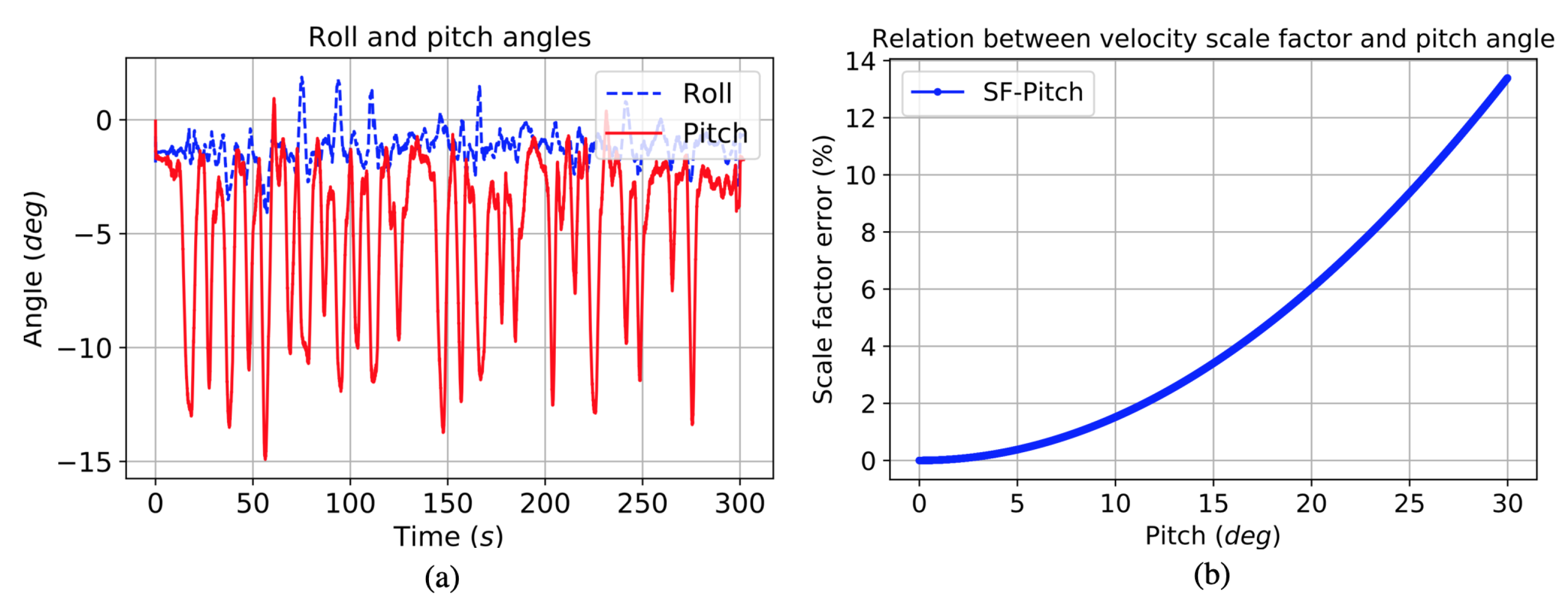
• According to the fact that the quadrotor may have a pitch angle when moving horizontally, the pitch angle, which is obtained from IMU and magnetometer data fusion, is used to set the weight of the forward velocity update.
• It is observed that the mass flow sensor may suffer from significant sensor errors, especially the scale factor error. Thus, a specific mass flow sensor calibration module is introduced.

This paper is organized as follows. Section 2 illustrates the methodology. Section 3 describes the experimental verification, and Section 4 draws the conclusions.

2. Methodology

Figure 1 illustrates the system diagram for the proposed multi-sensor integrated localization (MSL) method. The blue and red boxes indicate the inputs and outputs, respectively. The purple boxes represent the algorithm modules, while the green boxes indicate the prediction and update information for the MSL extended Kalman filter (EKF).

The IMU data are used for predicting the navigation states through the inertial navigation system (INS) mechanization and constructing the EKF system model. The magnetometer data are calibrated and utilized to compute the magnetometer heading, which is further used to build a heading update in the MSL EKF. The mass flow sensor data are calibrated and used in the velocity update in the EKF. The barometer data are used to detect height changes, which is in turn used for quality control (QC) on velocity updates. Meanwhile, the horizontal angles from IMU data are used for QC on velocity updates. The ultrasonic data are used to provide absolute position updates for the MSL EKF, so as to provide a reference location solution. The position data from the MSL EKF are also used to detect the outliers in ultrasonic position solutions. The following subsections separately describe the inertial navigation system (INS)-based attitude, velocity, and position prediction, the magnetometer heading update, the velocity update, the position update, and the EKF computation.

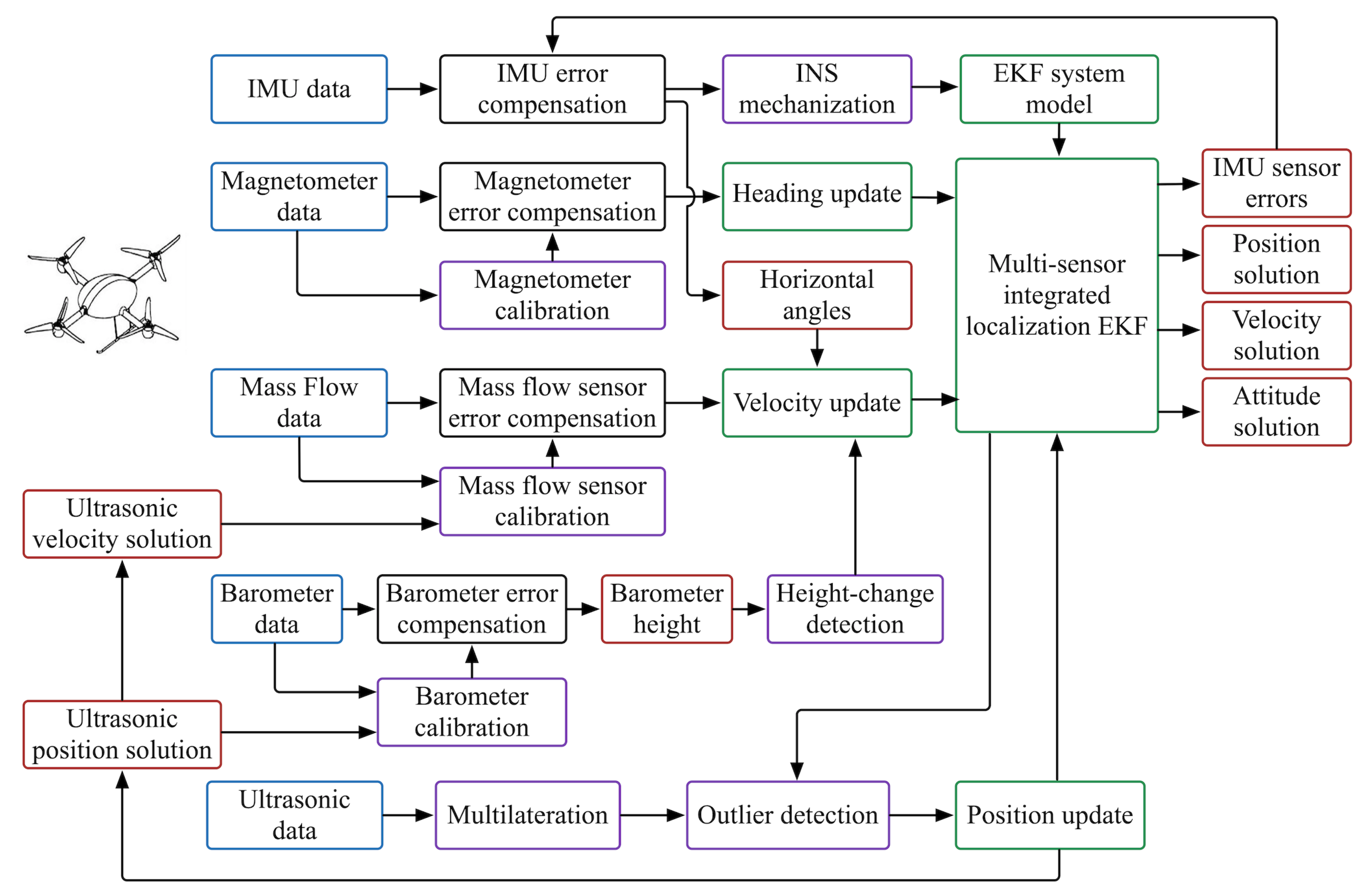
2.1. EKF System Model

Inertial navigation is a DR technique in which an IMU is tracked relative to its initial navigation states (i.e., attitude, velocity, and position) from the IMU body frame (i.e., b-frame) to the navigation frame (i.e., n-frame). The INS mechanization processes angular rates and specific forces (or angular and velocity increments) from gyros and accelerometers in the IMU for navigation-state prediction. Refer to Reference [44] for details about the INS mechanization. The predicted navigation states are also used to construct the MSL EKF system model. The INS error model [45] is applied in the continuous system model as

$${\dot{\mathbf{x}}}_{ms}={\mathbf{F}}_{ms}{\mathbf{x}}_{ms}+{\mathbf{w}}_{ms}$$

(1)

where ${\mathbf{x}}_{ms}$ and ${\mathbf{F}}_{ms}$ are the state vector and the dynamics matrix, respectively. ${\mathbf{w}}_{ms}$ is the system noise vector. The elements in the vectors and matrix are

$${\mathbf{x}}_{ms}={\left[\begin{array}{ccccc}\delta {\mathbf{p}}^n& \delta {\mathbf{v}}^n& \mathit{\psi }& {\mathbf{b}}_g& {\mathbf{b}}_a\end{array}\right]}^T$$

(2)

$$\begin{array}{c}\hfill {\mathbf{F}}_{ms}=\left[\begin{array}{ccccc}-[{\mathit{\omega }}_{en}^n\times ]& {\mathbf{I}}_{3\times 3}& {\mathbf{0}}_{3\times 3}& {\mathbf{0}}_{3\times 3}& {\mathbf{0}}_{3\times 3}\\ {\mathbf{0}}_{3\times 3}& -[(2{\mathit{\omega }}_{ie}^n+{\mathit{\omega }}_{en}^n)\times ]& [{\mathbf{f}}^n\times ]& {\mathbf{0}}_{3\times 3}& {\mathbf{C}}_b^n\\ {\mathbf{0}}_{3\times 3}& {\mathbf{0}}_{3\times 3}& -[({\mathit{\omega }}_{ie}^n+{\mathit{\omega }}_{en}^n)\times ]& -{\mathbf{C}}_b^n& {\mathbf{0}}_{3\times 3}\\ {\mathbf{0}}_{3\times 3}& {\mathbf{0}}_{3\times 3}& {\mathbf{0}}_{3\times 3}& -\frac{1}{{\tau }_{bg}}{\mathbf{I}}_{3\times 3}& {\mathbf{0}}_{3\times 3}\\ {\mathbf{0}}_{3\times 3}& {\mathbf{0}}_{3\times 3}& {\mathbf{0}}_{3\times 3}& {\mathbf{0}}_{3\times 3}& -\frac{1}{{\tau }_{ba}}{\mathbf{I}}_{3\times 3}\end{array}\right],{\mathbf{w}}_{ms}=\left[\begin{array}{c}{\mathbf{0}}_{3\times 1}\\ {\mathbf{C}}_b^n{\mathbf{w}}_a\\ -{\mathbf{C}}_b^n{\mathbf{w}}_g\\ {\mathbf{w}}_{bg}\\ {\mathbf{w}}_{ba}\end{array}\right]\end{array}$$

(3)

where the states $\delta {{p}}^n$, $\delta {\mathbf{v}}^n$, $\mathit{\psi }$, ${\mathbf{b}}_g$, and ${\mathbf{b}}_a$ are the vectors of position errors, velocity errors, attitude errors, gyro biases, and accelerometer biases, respectively; ${\mathit{C}}_b^n$ is the direction cosine matrix (DCM) from the b-frame to the n-frame. ${\mathbf{f}}^n$ is the specific force vector projected to the n-frame. The sign $[\mathbf{l}\times ]$ denotes the cross-product (skew-symmetric) form of the 3D vector $\mathbf{l}={\left[\begin{array}{ccc}{l}_1& l_2& l_3\end{array}\right]}^T$. ${\mathbf{w}}_g$ and ${\mathbf{w}}_a$ are noises in gyro and accelerometer readings, respectively; ${\tau }_{bg}$ and ${\tau }_{ba}$ denote the correlation time for ${\mathbf{b}}_g$ and ${\mathbf{b}}_a$, and ${\mathbf{w}}_{bg}$ and ${\mathbf{w}}_{ba}$ are the gyro and accelerometer bias driving noises. ${\mathbf{0}}_{3\times 3}$ and ${\mathbf{I}}_{3\times 3}$ are the 3D zero matrix and identity matrix, respectively.

2.2. Magnetometer Heading Update

In the INS mechanization, the horizontal attitude (i.e., roll and pitch) errors can be controlled by accelerometers, while the heading error may grow as a result of the weak observability of the heading angle and vertical gyro bias [41]. Thus, magnetometers are utilized to provide absolute heading updates. In indoor environments, the local magnetic field may be disturbed by man-made infrastructures. Therefore, calibration is required to use the magnetometer as a reliable source of heading. Refer to References [46,47] for magnetometer calibration and magnetometer heading computation, respectively. The calculated magnetometer heading are also fused with INS data in the attitude and heading reference system (AHRS) algorithm [48] to obtain the AHRS heading updates. The obtained heading is used to build the heading update model in the MSL EKF. The corresponding measurement model can be written as

$${\mathbf{z}}_{\psi ,k}={\mathbf{H}}_{\psi ,k}{\mathbf{x}}_{ms,k}+{\mathbf{v}}_{\psi ,k}$$

(4)

where ${\mathbf{z}}_{\psi ,k}$, ${\mathbf{H}}_{\psi ,k}$, and ${\mathbf{v}}_{\psi ,k}$ are the observation vector, design matrix, and measurement noise vector for heading update at time $t_k$. These vectors and matrix can be described as

$${\mathbf{z}}_{\psi ,k}={\psi }_{in,k}-{\psi }_{m,k}$$

(5)

$$\begin{array}{c}\hfill {\mathbf{H}}_{mc}=\left[\begin{array}{ccccc}{\mathbf{0}}_{1\times 3}& {\mathbf{0}}_{1\times 3}& \left[\begin{array}{ccc}0& 0& 1\end{array}\right]& {\mathbf{0}}_{1\times 3}& {\mathbf{0}}_{1\times 3}\end{array}\right]\end{array}$$

(6)

where ${\psi }_{m,k}$ is the magnetometer- or AHRS-derived heading at time $t_k$, and ${\psi }_{in,k}$ is the INS-predicted heading.

2.3. Velocity Update

It has been revealed in previous research that using a velocity update can enhance the heading observability when there are significant vehicle dynamics [42]. As illustrated in Section 1, this paper uses a velocity update and presents multiple updates for QC of velocity updates.

2.3.1. Velocity Update for Multi-Sensor Localization EKF

In this research, 3D velocity updates are applied. The forward velocity is measured by the mass flow sensor, while the lateral and vertical velocity components are set at zeroes plus noises. The corresponding MSL EKF measurement model can be written as

$${\mathbf{z}}_{vc,k}={\mathbf{H}}_{vc,k}{\mathbf{x}}_{ms,k}+{\mathbf{v}}_{vc,k}$$

(7)

where ${\mathbf{z}}_{vc,k}$, ${\mathbf{H}}_{vc,k}$, and ${\mathbf{v}}_{vc,k}$ are the observation vector, design matrix, and measurement noise vector for velocity update at time $t_k$. According to Reference [49], ${\mathbf{z}}_{vc}$ and ${\mathbf{H}}_{vc}$ can be written as

$${\mathbf{z}}_{vc}={\left({\mathbf{C}}_b^n\right)}^{-1}{\mathbf{v}}^n-{\tilde{\mathbf{v}}}^b$$

(8)

$$\begin{array}{c}\hfill {\mathbf{H}}_{vc}=\left[\begin{array}{ccccc}{\mathbf{0}}_{3\times 3}& {\left({\mathbf{C}}_b^n\right)}^{-1}& -{\left({\mathbf{C}}_b^n\right)}^{-1}[{\mathbf{v}}^n\times ]& {\mathbf{0}}_{3\times 3}& {\mathbf{0}}_{3\times 3}\end{array}\right]\end{array}$$

(9)

where ${\tilde{\mathbf{v}}}^b={\left[\begin{array}{ccc}{v}_f& 0& 0\end{array}\right]}^T$ and $v_f$ is the velocity from mass flow sensor.

2.3.2. Mass Flow Sensor Calibration

When the reference velocity form external technologies (e.g., ultrasonic) is available, the mass flow sensor can be calibrated. The velocity error model is

$$\tilde{v}=\frac{v_f-b_f}{s_f}$$

(10)

where $\tilde{v}$ is the reference velocity. $b_f$ and $s_f$ are the bias and scale factor of the mass flow sensor, respectively.

Thus, the mass flow sensor calibration model is

$${\mathbf{z}}_{fc}={\mathbf{H}}_{fc}{\mathbf{x}}_{fc}$$

(11)

where ${\mathbf{z}}_{fc}$, ${\mathbf{H}}_{fc}$, and ${\mathbf{x}}_{fc}$ are the observation vector, design matrix, and state vector for mass flow sensor calibration, and

$${\mathbf{x}}_{fc}={\left[\begin{array}{cc}\delta b_f& \delta s_f\end{array}\right]}^T$$

(12)

$$\begin{array}{c}\hfill {\mathbf{H}}_{fc}=\left[\begin{array}{cc}\frac{1}{s_f}& \frac{v_{f,1}-b_f}{s_f^2}\\ \dots & \dots \\ \frac{1}{s_f}& \frac{v_{f,i}-b_f}{s_f^2}\\ \dots & \dots \\ \frac{1}{s_f}& \frac{v_{f,N_{fc}}-b_f}{s_f^2}\end{array}\right]\end{array}$$

(13)

$${\mathbf{z}}_{fc}={\left[\begin{array}{ccccc}{v}_{f,1}-{\tilde{v}}_1& \dots & v_{f,i}-{\tilde{v}}_i& \dots & v_{f,N_{fc}}-{\tilde{v}}_{N_{fc}}\end{array}\right]}^T$$

(14)

where $N_{fc}$ is the number of mass flow sensor measurements.

The least squares method can be used to estimate ${\mathbf{x}}_{fc}$ by

$${\mathbf{x}}_{fc}={\left({\mathbf{H}}_{fc}^T{\mathbf{H}}_{fc}\right)}^{-1}{\mathbf{H}}_{fc}^T{\mathbf{z}}_{fc}.$$

(15)

The estimated mass flow sensor bias and scale factor errors are used to compensate for velocity errors before using the velocity update.

2.3.3. Availability for the Velocity Update

A QC mechanism is used to improve the robustness of velocity measurements. The basic ideas for QC include (1) the weight for the vertical velocity update is lowered when the vehicle has a significant height change and (2) the weight for the forward velocity update is decreased when the vehicle pitch angle is large. For (1), the barometer data are used for height change detection. With the model in Reference [50], the barometer-measured air pressure can be converted to the barometer height as

$$h_{b,k}=44330\left(1.0-{\left(\frac{100p_k}{p_0}\right)}^{\frac{1.0}{5.255}}\right)$$

(16)

where $h_{b,k}$ is the barometer height at time $t_k$, $p_k$ and $p_0$ are respectively the measured air pressure and the sea level reference pressure. The $p_0$ value is set at 101,325 Pa for calculation.

The height data are typically noisy. Thus, a smoother is used as

$$h_{b,k}=\sum _{i=1}^{n_{bs}}{c}_i{h}_{b,k-i+1}$$

(17)

where $n_{bs}$ is the smoother window size. $c_1$ to $c_{n_{bs}}$ are the coefficients that meet the condition ${\sum }_{i=1}^{n_{bs}}{c}_i=1$ and $c_1\ge \dots \ge c_{n_{bs}}$. This smoother causes a lag of $\frac{n_{bs}}{2}$ data epochs. Such a lag is acceptable for indoor UAVs because UAV sensors typically have a high data rate (e.g., over 50 Hz). A time lag of within 0.1 s will occur if $n_{bs}$ is set at 10.

The smoothed barometer height is used for tracking height changes through a threshold-based piecewise model. To use the method, a scoring value, ${\alpha }_{hc}$, is computed and compared with the corresponding threshold values. Specifically, when ${\alpha }_{hc}\le T_{hc,1}$ (i.e., the quasi-static-height mode), the vertical velocity measurement noise covariance is set at ${\sigma }_{vv}^2$. When $T_{hc,1}<{\alpha }_{hc}\le T_{hc,2}$ (i.e., the low-height-change mode), the vertical velocity measurement noise covariance is set at ${\left(\frac{{\alpha }_{hc}}{T_{hc,1}}{\sigma }_{vv}\right)}^2$. When ${\alpha }_{hc}>T_{hc,2}$ (i.e., the high-height-change mode), the vertical velocity measurement noise covariance is set at a large value ${\sigma }_{vmax}^2$. In this situation, the vertical velocity update will not contribute to the solution. To use the method, the standard deviation (STD) of the $n_h$ smoothed height data epochs is computed as the scoring value ${\alpha }_{hc}$. The threshold values are set based on training data.

For (2), a similar threshold-based piecewise model is used by comparing the real-time pitch angle to the preset threshold. Specifically, when $\theta \le T_{\theta ,1}$ (i.e., the horizontal mode), the forward velocity measurement noise covariance is set at ${\sigma }_{vf}^2$. When $T_{\theta ,1}<\theta \le T_{\theta ,2}$ (i.e., the low-pitch-angle mode), the forward velocity measurement noise covariance is set at ${\left(\frac{\theta }{T_{\theta ,1}}{\sigma }_{vf}\right)}^2$. When $\theta >T_{\theta ,2}$ (i.e., the high-pitch-angle mode), the forward velocity measurement noise covariance is set at a large value ${\sigma }_{vmax}^2$.

2.4. Position Update

Although the integration of data from the IMU, magnetometers, barometer, and mass flow sensor can provide a short-term accurate DR solution, the solution will drift over time when an absolute update is not available. The drifts of the navigation solution will occur especially when low-cost MEMS sensors are used, since these sensors are susceptible to significant run-to-run biases and thermal drifts. Thus, to obtain a long-term accurate navigation solution, at least one type of the absolute updates is required. In this research, the device-anchor ranges from ultrasonic sensors are used to integrate with MSL EKF, so as to obtain references for the localization solution.

Ultrasonic sensors can provide accurate (i.e., centimeter-level) ranges in environments that have clear line-of-sight between the device and anchors. However, the ranging accuracy may be degraded by outliers that may occur as a result of obstructions between the device and anchors and the multipath effect. This section describes the method for localization using ultrasonic ranges, the position measurement model for the MSL EKF, and the method for removing outliers in ultrasonic ranges.

2.4.1. Ultrasonic Multilateration

For 3D localization, the model for the range between the device and the i-th anchor is

$$d_i=\sqrt{({(x_i-x_r)}^2+{(y_i-y_r)}^2+{(z_i-z_r)}^2).}$$

(18)

Therefore, the multilateration model is

$$\begin{array}{c}\hfill {\mathbf{z}}_r={\mathbf{H}}_r{\mathbf{x}}_r\end{array}$$

(19)

where ${\mathbf{x}}_r=\left[\begin{array}{ccc}\delta x& \delta y& \delta z\end{array}\right]$ represents the vector of device location errors, ${\mathbf{z}}_r$ is the observation vector for multilateration, ${\mathbf{H}}_r$ is the design matrix for multilateration, and

$$\begin{array}{c}\hfill {\mathbf{H}}_r=\left[\begin{array}{ccc}\frac{x_r-x_1}{d_1}& \frac{y_r-y_1}{d_1}& \frac{z_r-z_1}{d_1}\\ \dots & \dots \\ \frac{x_r-x_i}{d_i}& \frac{y_r-y_i}{d_i}& \frac{z_r-z_i}{d_i}\\ \dots & \dots \\ \frac{x_r-x_{N_r}}{d_{N_r}}& \frac{y_r-y_{N_r}}{d_{N_r}}& \frac{z_r-z_{N_r}}{d_{N_r}}\end{array}\right]\end{array}$$

(20)

$$\begin{array}{c}\hfill {\mathbf{z}}_r={\left[\begin{array}{ccccc}{\tilde{d}}_1-d_1& \dots & {\tilde{d}}_i-d_i& \dots & {\tilde{d}}_{N_r}-d_{N_r}\end{array}\right]}^T.\end{array}$$

(21)

The state vector ${\mathbf{x}}_r$ is estimated by

$${\widehat{\mathbf{x}}}_r={\left({\mathbf{H}}_r^T{\mathbf{H}}_r\right)}^{-1}{\mathbf{H}}_r^T{\mathbf{z}}_r$$

(22)

where ${\mathbf{x}}_r={\left[\begin{array}{ccc}{x}_r& y_r& z_r\end{array}\right]}^T$ and $x_r$, $y_r$, and $z_r$ are the device coordinates along east, north, and up directions.

2.4.2. Position Update for Multi-Sensor Localization EKF

The ultrasound-derived position solutions are used to build the MSL EKF position update model as

$${\mathbf{z}}_{pc,k}={\mathbf{H}}_{pc,k}{\mathbf{x}}_{ms,k}+{\mathbf{v}}_{pc,k}$$

(23)

where ${\mathbf{z}}_{pc,k}$, ${\mathbf{H}}_{pc,k}$, and ${\mathbf{v}}_{pc,k}$ are the observation vector, design matrix, and measurement noise vector for position update at time $t_k$, and

$${\mathbf{z}}_{pc,k}={\left[\begin{array}{ccc}(R_m+h)({\chi }_k-{\chi }_{ref})-{\tilde{x}}_k& (R_n+h)({\beta }_k-{\beta }_{ref})cos{\chi }_k-{\tilde{y}}_k& h_k-h_{ref}-{\tilde{z}}_k\end{array}\right]}^T$$

(24)

$$\begin{array}{c}\hfill {\mathbf{H}}_{pc,k}=\left[\begin{array}{ccccc}\Lambda \left(\left[\begin{array}{ccc}(R_m+h)& (R_n+h)cos{\chi }_k& 1\end{array}\right]\right)& {\mathbf{0}}_{3\times 3}& {\mathbf{0}}_{3\times 3}& {\mathbf{0}}_{3\times 3}& {\mathbf{0}}_{3\times 3}\end{array}\right]\end{array}$$

(25)

where ${\left[\begin{array}{ccc}{\tilde{x}}_k& {\tilde{y}}_k& {\tilde{z}}_k\end{array}\right]}^T$ is the multilateration solution using ultrasonic ranges at time $t_k$. ${\left[\begin{array}{ccc}{\chi }_k& {\beta }_k& h_k\end{array}\right]}^T$ are the elements in ${\mathbf{p}}^n$. ${\left[\begin{array}{ccc}{\chi }_{ref}& {\beta }_{ref}& h_{ref}\end{array}\right]}^T$ is the global position (i.e., latitude, longitude, and ellipsoidal height) of the original point for the local coordinate frame (i.e., x, y, and z).

2.4.3. Ultrasonic Position Outlier Detection

To detect outliers in ultrasonic positioning solutions, statistical testing is implemented on the innovations of the MSL EKF. The innovation sequence and its covariance matrix can be calculated by [51]

$${\mathsf{\xi }}_k={\mathbf{z}}_{pc,k}-{\mathbf{H}}_{pc,k}{\mathbf{x}}_{ms,k}$$

(26)

$${\mathbf{C}}_{{\xi }_k}={\mathbf{H}}_{pc,k}{\mathbf{P}}_{ms,k}{\mathbf{H}}_{pc,k}^T+{\mathbf{R}}_{pc,k}$$

(27)

where ${\mathbf{P}}_{ms,k}$ is the state covariance matrix in the MSL EKF and ${\mathbf{R}}_{pc,k}$ is the position measurement covariance matrix. The assumption for outlier detection is

$$H_0:\frac{{\xi }_{k,i}}{\sqrt{{\mathbf{C}}_{{\xi }_k}\left[i\right]\left[i\right]}}\sim N(0,1)$$

(28)

where ${\mathbf{C}}_{{\xi }_k}\left[i\right]\left[i\right]$ is the element at row i column i of ${\mathbf{C}}_{{\xi }_k}$. $N(c_1,c_2)$ represents the normal distribution with mean of $c_1$ and covariance of $c_2$. If the hypothesis is rejected, the measurements corresponding to the outliers are removed.

With the system model and measurement models, the EKF predicts the states and then obtains updates from noisy measurements. Refer to Reference [45] for details of EKF computation.

3. Tests and Results

3.1. Test Description

To verify the proposed MSL method, indoor flight tests were conducted with a 3DR Solo quadrotor [52]. Figure 2a illustrates the test environment (20 m × 20 m) and Figure 2b shows the quadrotor and sensors. Five Marvelmind ultrasonic (abbreviated as US) beacons [53] were used, including one fixed on the quadrotor and four installed on four static leveling pillars. The height of the four static beacons was 4 m.

The quadrotor was equipped with an InvenSense MPU6000 MEMS-based IMU [54], a Honeywell HMC 5983 magnetometer (abbreviated as Mag) triad [55], a TE MS5611 barometer (abbreviated as Baro) [56], a Sensirion SFM3000 mass flow sensor (abbreviated as Flow) [57], and a Marvelmind US beacon. The data rates for IMU, Mag, Baro, Flow, and US were 50, 100, 100, 100, and 100 Hz, respectively. A LattePanda 4 GB/64 GB Windows 10 single board computer was used for data collection and sensor fusion computation [58].

Four flying tests with various quadrotor trajectories were conducted. The trajectories are shown by blue lines in Figure 3. Each trajectory lasted for five to ten minutes. The locations of four US anchors are shown by red pins in Figure 3. The reference trajectories were obtained by post-processing of fusing US with INS, Mag, Baro, and Flow data. The used US system can provide a centimeter-level ranging accuracy in line-of-sight environments [53].

3.2. Impact of Velocity Solutions

In this subsection, the impact of the velocity update is tested. Meanwhile, other factors, such as the detection of height changes and the pitch angle, are investigated. Finally, the AHRS/INS/Velocity integrated solutions that use various velocity strategies are evaluated.

3.2.1. Velocity Solutions (Mass Flow-Based)

To investigate the effect of mass flow sensor calibration, Figure 4a illustrates the raw and low-pass filtered mass flow data, as well as the reference 1D velocity from ultrasonic solutions. There was a difference between the filtered and reference data, which indicated the existence of mass flow sensor errors. Such data were used as training data for mass flow sensor calibration.

The estimated mass flow sensor bias and scale factor values were further used to compensate the mass flow data in the tests. The corresponding 1D velocity time series are shown in Figure 4b. Compared to the filtered velocity, the calibrated velocity was closer to the reference. This phenomenon indicates the effectiveness of mass flow sensor calibration.

3.2.2. Height-Change Detection (Barometer-Based)

The barometer height was utilized to detect the time periods that did not have a significant height change. These time periods were important for using the vertical velocity update. Figure 5 illustrates the raw and smoothed barometer heights, as well as the indicator for the time periods that did not have a significant height change. The time periods indicated by the cyan dots that had a legend of Flag-H.

The data in Figure 5 indicate that even when the quadrotor is controlled to move horizontally, it may have height changes. With the height-change detection technique, it is possible to process the barometer data to obtain the time periods during which the quadrotor had only horizontal movements.

According to training data, the $n_h$ value was set at 50 (i.e., barometer data epochs in half a second), the height-change threshold values $T_{hc,1}$ and $T_{hc,2}$ were set at 0.02 m and 0.06 m, respectively. The vertical velocity covariance values ${\sigma }_{vv}^2$ and ${\sigma }_{vmax}^2$ were set at (0.1 m/s)${}^2$ and (100 m/s)${}^2$, respectively.

3.2.3. Impact of Pitch Angle on Velocity

In contrast to land vehicles, quadrotors may have significant horizontal angles, especially the pitch angle, during the flying process. Figure 6a illustrates the roll and pitch angle during a test. The pitch angle reached 15 deg. Figure 6b shows the theoretical relationship between the pitch angle and the forward velocity scale factor error. A scale factor error of around 4 % may be introduced by a pitch angle of 15 deg.

According to the training data, the pitch-angle threshold values $T_{\theta ,1}$ and $T_{\theta ,2}$ were set at 10 deg and 30 deg, respectively. The forward velocity covariance value ${\sigma }_{vf}^2$ was set at (0.3 m/s)${}^2$.

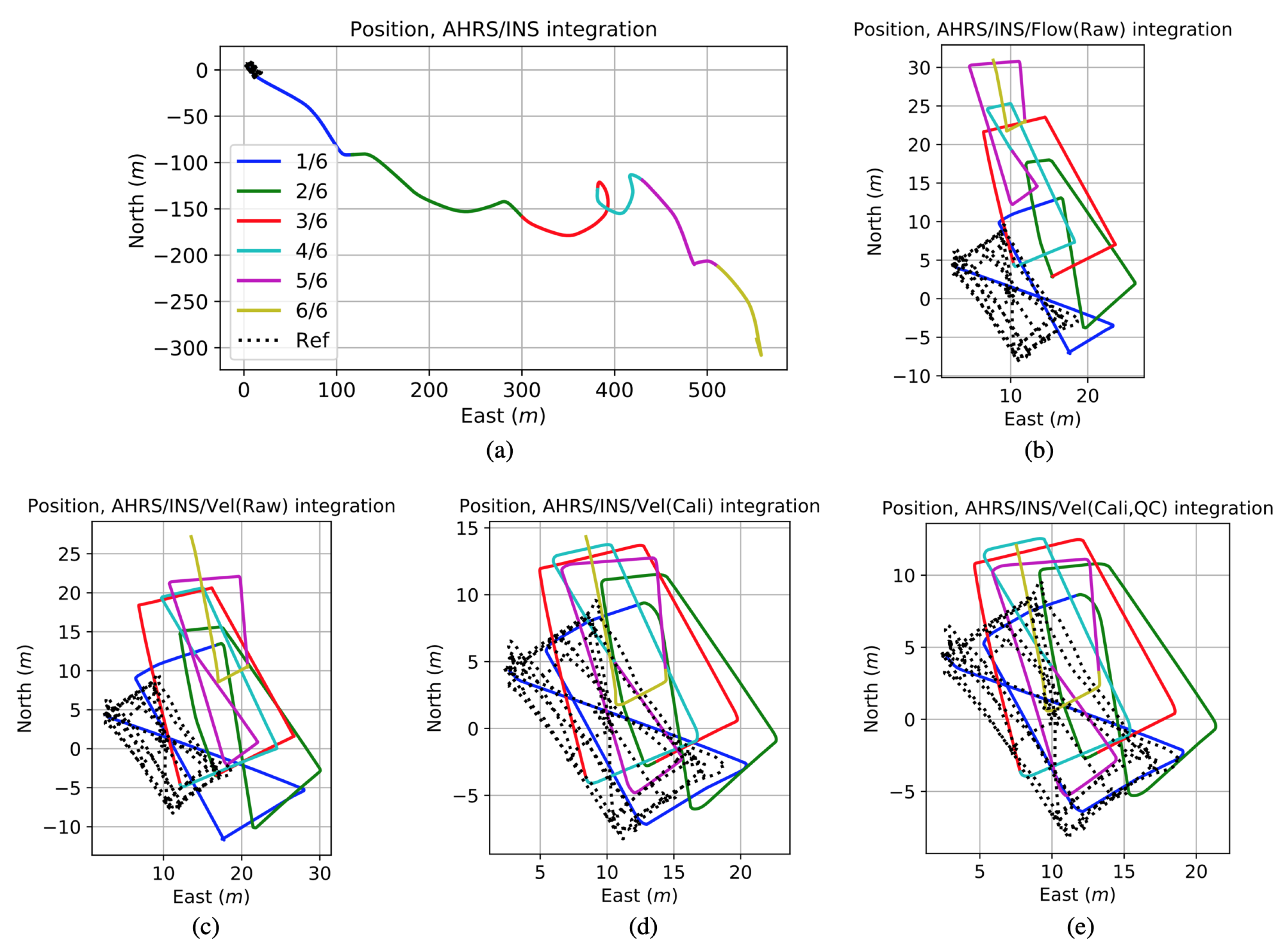
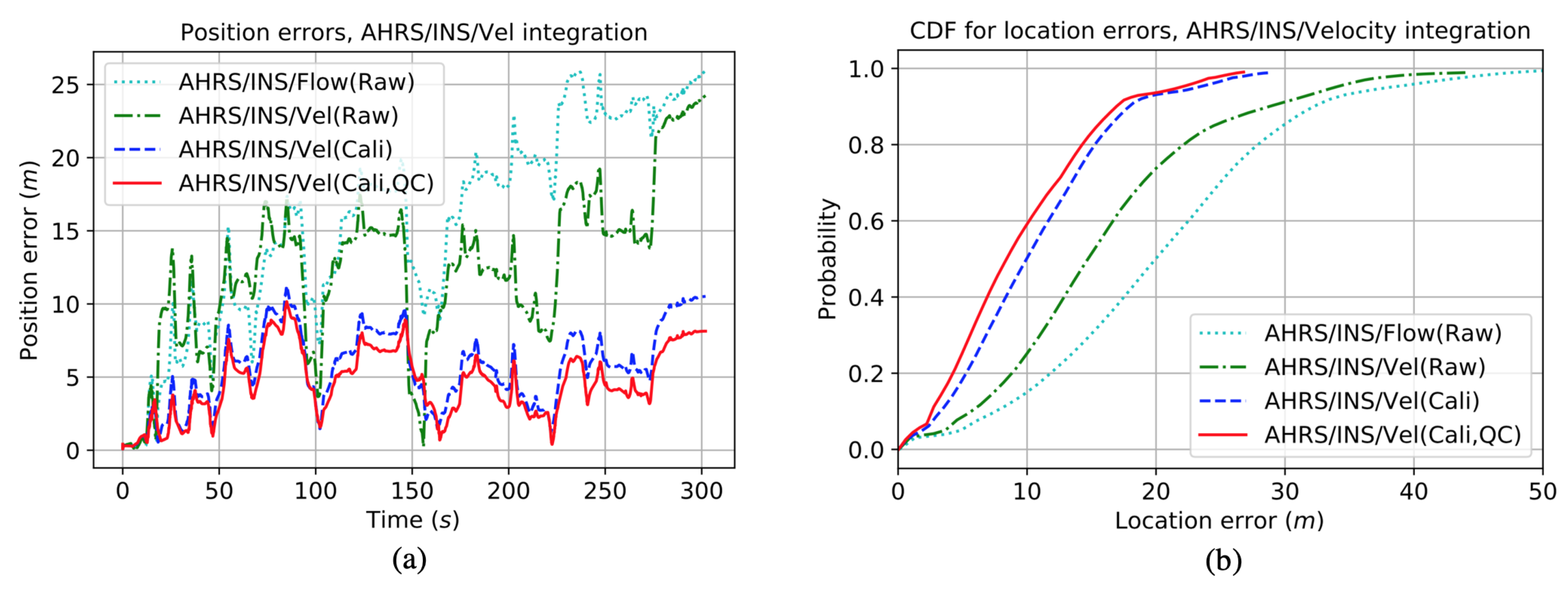
3.2.4. AHRS/INS/Velocity Integrated Solutions with Various Velocity Strategies

Figure 7 shows the position solutions from the following strategies:

• AHRS/INS: integration of AHRS heading and INS mechanization, without using any velocity update.
• AHRS/INS/Flow(Raw): using raw mass flow sensor data (i.e., 1D velocity) as the update in the MSL EKF.
• AHRS/INS/Vel(Raw): using raw mass flow sensor data and NHC for 3D velocity updates in the MSL EKF.
• AHRS/INS/Vel(Cali): using calibrated mass flow sensor data and NHC (i.e., 3D velocity) in the MSL EKF.
• AHRS/INS/Vel(Cali,QC): using mass flow sensor data that were calibrated and had QC based on height-change and pitch-angle detection, as well as NHC (i.e., 3D velocity) in the MSL EKF.

Figure 7 indicates the importance of using proper velocity updates on motion-sensor-based quadrotor localization. Figure 8a,b shows the location error time series of the strategies that had velocity updates in one test, and the cumulative distribution function (CDF) of location errors in all four tests.

Table 2. Statistics of AHRS/INS/Velocity integrated location errors, with various velocity strategies.

Strategy	Mean	RMS	80%	95%	Max
AHRS/INS (m)	415.6	475.7	632.6	792.9	966.0
AHRS/INS/Flow(Raw) (m)	20.2	22.4	27.6	38.4	58.4
AHRS/INS/Vel(Raw) (m)	15.9	18.1	21.6	32.9	44.3
AHRS/INS/Vel(Cali) (m)	10.6	12.1	15.5	23.8	28.9
AHRS/INS/Vel(Cali,QC) (m)	9.4	11.0	14.8	22.4	26.8
${\nabla }_{AHRS/INS}^{AHRS/INS/Flow\left(Raw\right)}$	95.1%	95.3%	95.6%	95.2%	94.0%
${\nabla }_{AHRS/INS/Flow\left(Raw\right)}^{AHRS/INS/Vel\left(Raw\right)}$	21.3%	19.2%	21.7%	14.3%	24.1%
${\nabla }_{AHRS/INS/Vel\left(Raw\right)}^{AHRS/INS/Vel\left(Cali\right)}$	33.3%	33.1%	28.2%	27.7%	34.7%
${\nabla }_{AHRS/INS/Vel\left(Cali\right)}^{AHRS/INS/Vel(Cali,QC)}$	11.3%	9.1%	4.5%	5.9%	7.3%

${\nabla }_b^a$: improvement of solution a over solution b.

illustrates the location error statistics, including the mean, root mean squares (RMS), 80% and 95% quantile errors, and the maximum value.

Compared to AHRS/INS/Flow(Raw), the mean AHRS/INS/Vel(Raw) location error was reduced from 20.2 m to 15.9 m, with an accuracy improvement of 21.3%. This phenomenon indicates the benefits of using 3D velocity instead of 1D.

When using the calibrated mass flow data, the location error mean value in AHRS/INS/Vel(Cali) was reduced to 10.6 m, which was 33.3% lower than that in AHRS/INS/Vel(Raw). Such accuracy improvement is significant, which suggest calibration for the mass flow sensor. The AHRS/INS/ Vel(Cali,QC) strategy further reduced the mean location error from 10.6 m to 9.4 m, with an accuracy improvement of around 10%.

3.3. Integrated Localization Solutions during Ultrasonic Positioning Signal Outages

3.3.1. Use of Ultrasonic Positioning

The solutions in Section 3.2 indicate the effectiveness of using more reliable velocity solutions in enhancing AHRS/INS/Velocity integrated navigation. On the other hand, it is shown that it was challenging to obtain a long-term DR solution with such an AHRS/INS/Velocity integrated system on a quadrotor. Thus, external updates are still needed. Figure 9 shows the US position solution that was obtained through the method in Section 2.4.1. Figure 9a demonstrates the time series of the ranges from the quadrotor to four anchors. Figure 9b,c shows the 2D location solution and the east and north positions, and Figure 9d illustrates the height solution.

The US system can provide a centimeter-level ranging accuracy [53]; thus, the multilateration solution was expect to be generally at a centimeter to decimeter level, which was at least one level more accurate than the DR position accuracy (sub-meter to meter level). One issue for the US positioning system is that there were outliers in range measurements, which caused outliers in the US position solution in Figure 9a.

3.3.2. AHRS/INS/Velocity/Ultrasonic Integrated Solution

To mitigate the effect of outliers, the US positioning solution was utilized as the position update for the MSL EKF by following the method in Section 2.4.2. The outliers were detected and removed by using the approach in Section 2.4.3. Figure 10a–d demonstrate the 2D locations, east and north positions, 1D velocity magnitude, and the east and north velocity components from the MSL EKF, respectively. Compared to the solution in Figure 9, the position solutions became smoother, with all position outliers removed. The MSL EKF position solutions were used as the reference trajectories to evaluate the MSL solution during US signal outages in the next subsection.

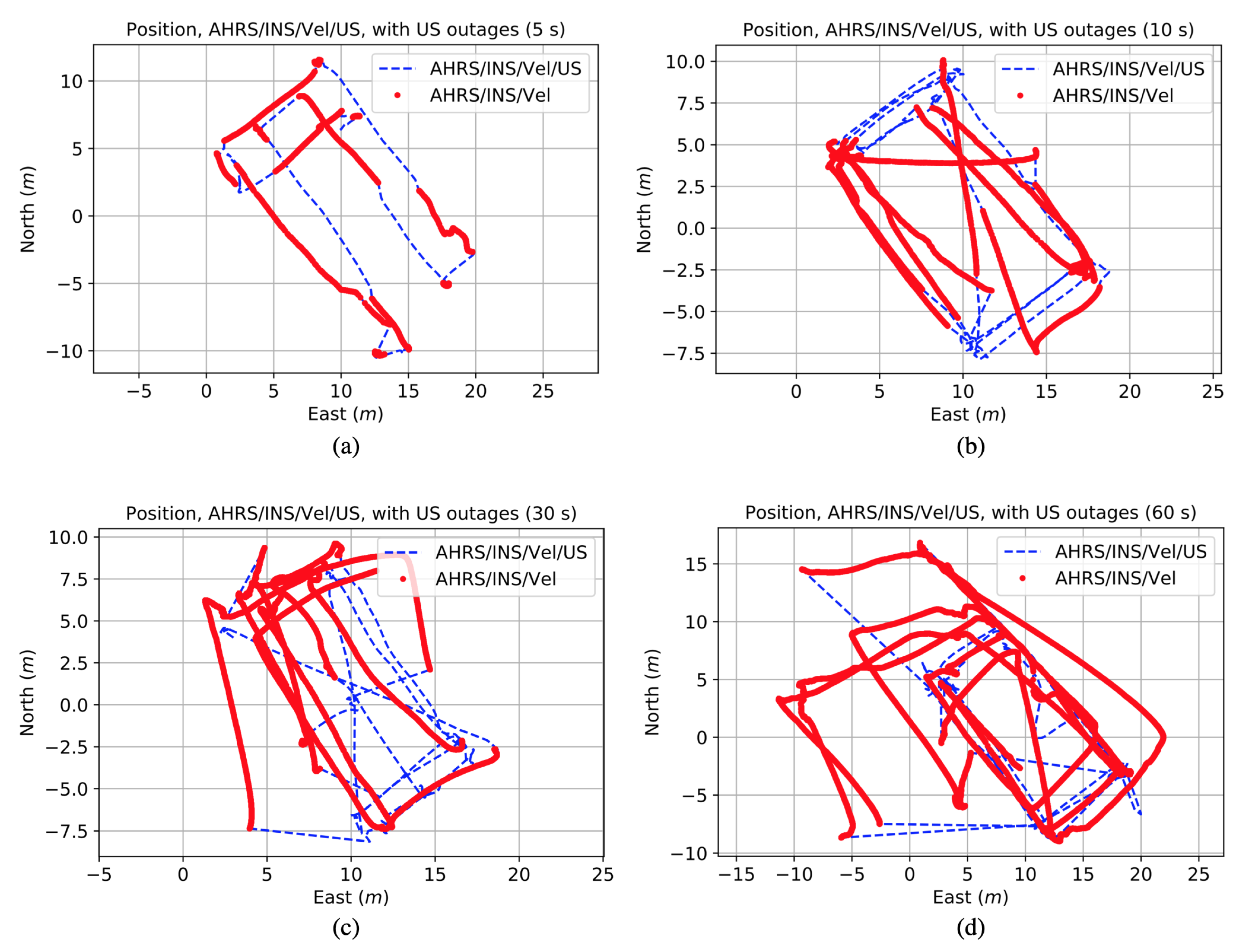
3.3.3. AHRS/INS/Velocity Integrated Solution during US Outages

To focus on AHRS/INS/Velocity localization, the US positions were cut off to generate US outages. The US outage time length was set at various values (e.g., 5, 10, 15, 20, 30, and 60 s), so as to investigate the AHRS/INS/Velocity solution for different time periods. The AHRS/INS/Velocity system will be valuable in engineering practices if it can provide a reliable solution during US position outages.

Figure 11a–d shows the 2D position results by processing four sets of test data with US outages of 5, 10, 30, and 60 s, respectively. The red dots indicates the solutions during US outage time periods. Figure 12a illustrates the east and north positions with and without US outages, and Figure 12b shows the corresponding location errors, which were the differences between the results with and without US outages. Thus, in Figure 12b, the location errors during the time periods that had US position updates were not used when computing the location error statistics in this subsection.

Figure 11 and Figure 12 indicate that the location errors drifted over time during US outage periods. The maximum drifts reached 1.3, 3.0, 7.2, and 17.7 m in the selected test data that had US outages of 5, 10, 30, and 60 s, respectively.

Figure 13a illustrates the CDF of 2D location errors when using US outage time periods of 5, 10, 15, 20, 30, and 60 s on all test trajectories. Only the location errors during US outage periods were used for calculation. Figure 13b shows the corresponding statistics.

According to Figure 13b, the mean 2D location errors were 0.2, 0.6, 1.0, 1.3, 1.8, and 4.3 m when there were US outages of 5, 10, 15, 20, 30, and 60 s, respectively. This solution indicated that the AHRS/INS/Velocity integrated system generally provided a localization accuracy (in mean value) of approximately 1.0 m and 2.0 m when localizing using AHRS/INS/Velocity integration for 15 and 30 s, respectively. Such location accuracy is acceptable because one-meter accuracy for 15 s is enough for resisting many signal interference and outages for a commercial US system. Particularly, the location accuracy reached 0.2 and 0.6 m when localizing using AHRS/INS/Velocity integration for 5 and 10 s, respectively. Such accuracy was promising for self-contained quadrotor localization without using high-precision wireless or vision localization technologies.

4. Conclusions

This paper has investigated the integration of low-cost IMU, magnetometer, barometer, and mass flow sensors for quadrotor UAV localization. Multiple indoor flying tests were conducted using ultrasonic ranging measurements to compute the reference trajectories. The introduction of forward velocity from the mass flow sensor improved the AHRS/INS-based DR location accuracy (in mean value) by 95.0%, and the use of 3D velocity updates further enhanced the location accuracy by 21.3%. Furthermore, the calibration of mass flow sensor improved the location accuracy by 33.3%, and the sensor interaction strategies further enhanced the location accuracy by 11.3%. The proposed AHRS/INS/Velocity integrated approach generally provided a localization accuracy of 0.2, 0.6, 1.0, 1.3, 1.8, and 4.3 m when localizing for 5, 10, 15, 20, 30 and 60 s, respectively. Such DR accuracy (1.0 m for 15 s and 1.8 m for 30 s) was promising to bridge the signal outages from high-precision localization technologies and to resist outliers in the high-precision localization data.

References

1. Feng, Q.; Liu, J.; Gong, J. UAV Remote Sensing for Urban Vegetation Mapping Using Random Forest and Texture Analysis. Remote Sens. 2015, 7, 1074–1094. [Google Scholar] [CrossRef] [Green Version]
2. Chen, S.; Guo, S.; Li, Y. Real-time tracking a ground moving target in complex indoor and outdoor environments with UAV. In Proceedings of the IEEE International Conference on Information and Automation (ICIA), Ningbo, China, 1–3 August 2016; pp. 362–367. [Google Scholar]
3. Kobayashi, T.; Seimiya, S.; Harada, K.; Noi, M.; Barker, Z.; Woodward, G.; Willig, A.; Kohno, R. Wireless technologies to assist search and localization of victims of wide-scale natural disasters by unmanned aerial vehicles. In Proceedings of the International Symposium on Wireless Personal Multimedia Communications (WPMC), Bali, Indonesia, 17–20 December 2017; pp. 404–410. [Google Scholar]
4. Wu, K.; Gregory, T.; Moore, J.; Hooper, B.; Lewis, D.; Tse, Z. Development of an indoor guidance system for unmanned aerial vehicles with power industry applications. IET Radar Sonar Navig. 2017, 11, 212–218. [Google Scholar] [CrossRef]
5. Gao, Z.; Li, Y.; Zhuang, Y.; Yang, H.; Pan, Y.; Zhang, H. Robust Kalman Filter Aided GEO/IGSO/GPS Raw-PPP/INS Tight Integration. Sensors 2019, 19, 417. [Google Scholar] [CrossRef] [PubMed]
6. Burdziakowski, P. Towards Precise Visual Navigation and Direct Georeferencing for MAV Using ORB-SLAM2. In Proceedings of the Baltic Geodetic Congress (BGC Geomatics), Gdansk, Poland, 22–25 June 2017; pp. 394–398. [Google Scholar]
7. Valenti, F.; Giaquinto, D.; Musto, L.; Zinelli, A.; Bertozzi, M.; Broggi, A. Enabling Computer Vision-Based Autonomous Navigation for Unmanned Aerial Vehicles in Cluttered GPS-Denied Environments. In Proceedings of the IEEE International Conference on Intelligent Transportation Systems (ITSC), Maui, HI, USA, 4–7 November 2018. [Google Scholar] [CrossRef]
8. Chen, Z.; Wang, C.; Wang, H.; Ma, Y.; Liang, G.; Wu, X. Heterogeneous Sensor Information Fusion based on Kernel Adaptive Filtering for UAVs’ Localization. In Proceedings of the IEEE International Conference on Information and Automation (ICIA), Macau, China, 18–20 July 2017; pp. 171–176. [Google Scholar]
9. Bulunseechart, T.; Smithmaitrie, P. A method for UAV multi-sensor fusion 3D-localization under degraded or denied GPS situation. J. Unmanned Veh. Syst. 2018, 6, 155–176. [Google Scholar] [CrossRef]
10. Nahangi, M.; Heins, A.; McCabe, B.; Schoellig, A.P. Automated Localization of UAVs in GPS-Denied Indoor Construction Environments Using Fiducial Markers. In Proceedings of the 35th ISARC, Berlin, Germany, 20–25 July 2018; pp. 88–94. [Google Scholar]
11. Santos, M.; Santana, L.; Brandão, A.; Sarcinelli-Filhod, M.; Carellie, R. Indoor low-cost localization system for controlling aerial robots. Control Eng. Pract. 2017, 61, 93–111. [Google Scholar] [CrossRef]
12. Qi, J.; Yu, N.; Lu, X. A UAV positioning strategy based on optical flow sensor and inertial navigation. In Proceedings of the IEEE International Conference on Unmanned Systems (ICUS), Beijing, China, 27–29 October 2017; pp. 81–87. [Google Scholar]
13. Walter, V.; Saska, M.; Franchi, A. Fast Mutual Relative Localization of UAVs using Ultraviolet LED markers. In Proceedings of the International Conference on Unmanned Aircraft Systems, Dallas, TX, USA, 12–15 June 2018; pp. 1217–1226. [Google Scholar]
14. Li, K.; Wang, C.; Huang, S.; Liang, G.; Wu, X.; Liao, Y. Self-positioning for UAV indoor navigation based on 3D laser scanner, UWB and INS. In Proceedings of the IEEE International Conference on Information and Automation (ICIA), Ningbo, China, 1–3 August 2016; pp. 498–503. [Google Scholar]
15. Li, J.; Zhan, H.; Chen, B.; Reid, I.; Lee, G. Deep learning for 2D scan matching and loop closure. In Proceedings of the IEEE/RSJ International Conference on Intelligent Robots and Systems (IROS), Vancouver, BC, Canada, 24–28 September 2017; pp. 763–768. [Google Scholar]
16. Opromolla, R.; Fasano, G.; Rufino, G.; Grassi, M.; Savvaris, A. Lidar-inertial integration for UAV localization and mapping in complex environments. In Proceedings of the International Conference on Unmanned Aircraft Systems (ICUAS), Arlington, VA, USA, 7–10 June 2016; pp. 649–656. [Google Scholar]
17. Yuan, C.; Lai, J.; Zhang, J.; Lyu, P. Research on an autonomously tightly integrated positioning method for UAV in sparse-feature indoor environment. In Proceedings of the International Bhurban Conference on Applied Sciences and Technology (IBCAST), Islamabad, Pakistan, 9–13 January 2018; pp. 318–324. [Google Scholar]
18. Bavle, H.; Sanchez-Lopez, J.; Rodriguez-Ramos, A.; Sampedro, C.; Campoy, P. A flight altitude estimator for multirotor UAVs in dynamic and unstructured indoor environments. In Proceedings of the International Conference on Unmanned Aircraft Systems (ICUAS), Miami, FL, USA, 13–16 June 2017; pp. 1044–1051. [Google Scholar]
19. Scannapieco, A.; Renga, A.; Fasano, G.; Moccia, A. Experimental Analysis of Radar Odometry by Commercial Ultralight Radar Sensor for Miniaturized UAS. J. Intell. Robot. Syst. 2018, 90, 485–503. [Google Scholar] [CrossRef]
20. Zahran, S.; Mostafa, M.; Masiero, A.; Moussa, A.; Vettore, A.; El-Sheimy, N. Micro-radar and uwb aided uav navigation in gnss denied environment, Int. Arch. Photogramm. Remote Sens. Spat. Inf. Sci. 2018, 42, 469–476. [Google Scholar]
21. Cisek, K.; Zolich, A.; Klausen, K.; Johansen, T. Ultra-wide band Real time Location Systems: Practical implementation and UAV performance evaluation. In Proceedings of the Workshop on Research, Education and Development of Unmanned Aerial Systems (RED-UAS), Linkoping, Sweden, 3–5 October 2017; pp. 204–209. [Google Scholar]
22. Tiemann, J.; Wietfeld, C. Scalable and precise multi-UAV indoor navigation using TDOA-based UWB localization. In Proceedings of the International Conference on Indoor Positioning and Indoor Navigation (IPIN), Sapporo, Japan, 18–21 September 2017; pp. 1–7. [Google Scholar]
23. Miraglia, G.; Maleki, K.; Hook, L. Comparison of two sensor data fusion methods in a tightly coupled UWB/IMU 3-D localization system. In Proceedings of the International Conference on Engineering, Technology and Innovation (ICE/ITMC), Funchal, Portugal, 27–29 June 2017; pp. 611–618. [Google Scholar]
24. Tiemann, J.; Ramsey, A.; Wietfeld, C. Enhanced UAV Indoor Navigation through SLAM-Augmented UWB Localization. In Proceedings of the IEEE International Conference on Communications Workshops (ICC Workshops), Kansas City, MO, USA, 20–24 May 2018; pp. 1–6. [Google Scholar]
25. Perez-Grau, F.; Caballero, F.; Merino, L.; Viguria, A. Multi-modal mapping and localization of unmanned aerial robots based on ultra-wideband and RGB-D sensing. In Proceedings of the IEEE/RSJ International Conference on Intelligent Robots and Systems (IROS), Vancouver, BC, Canada, 24–28 September 2017; pp. 3495–3502. [Google Scholar]
26. Kapoor, R.; Ramasamy, S.; Gardi, A.; Sabatini, R. Indoor navigation using distributed ultrasonic beacons. In Proceedings of the 17th Australian International Aerospace Congress (AIAC17), Melbourne, Australia, 26–28 February 2017; pp. 551–556. [Google Scholar]
27. Kang, D.; Cha, Y. Autonomous UAVs for Structural Health Monitoring Using Deep Learning and an Ultrasonic Beacon System with Geo-Tagging. Comput.-Aided Civ. Infrastruct. Eng. 2018, 33, 885–902. [Google Scholar] [CrossRef]
28. Paredes, J.A.; Alvarez, F.J.; Aguilera, T.; Villadangos, J.M. 3D Indoor Positioning of UAVs with Spread Spectrum Ultrasound and Time-of-Flight Cameras. Sensors 2018, 18, 89. [Google Scholar] [CrossRef]
29. Zou, H.; Jin, M.; Jiang, H.; Xie, L.; Spanos, C. WinIPS: WiFi-Based Non-Intrusive Indoor Positioning System With Online Radio Map Construction and Adaptation. IEEE Trans. Wirel. Commun. 2017, 16, 8118–8130. [Google Scholar] [CrossRef]
30. Tian, X.; Song, Z.; Jiang, B.; Zhang, Y.; Yu, T.; Wang, X. HiQuadLoc: A RSS Fingerprinting Based Indoor Localization System for Quadrotors. IEEE Trans. Mob. Comput. 2017, 16, 2545–2559. [Google Scholar] [CrossRef]
31. Zhou, M.; Lin, J.; Liang, S.; Du, W.; Cheng, L. A UAV patrol system based on Bluetooth localization. In Proceedings of the Asia-Pacific Conference on Intelligent Robot Systems (ACIRS), Wuhan, China, 16–18 June 2017; pp. 205–209. [Google Scholar]
32. Won, D.; Park, M.; Chi, S. Construction Resource Localization Based on UAV-RFID Platform Using Machine Learning Algorithm. In Proceedings of the IEEE International Conference on Industrial Engineering and Engineering Management (IEEM), Bangkok, Thailand, 16–19 December 2018; pp. 1086–1090. [Google Scholar] [CrossRef]
33. Brzozowski, B.; Kaźmierczak, K.; Rochala, Z.; Wojda, M.; Wojtowicz, K. A concept of UAV indoor navigation system based on magnetic field measurements. Proceedngs of the IEEE Metrology for Aerospace (MetroAeroSpace), Florence, Italy, 22–23 June 2016; pp. 636–640. [Google Scholar]
34. Zahran, S.; Moussa, A.; Sesay, A.; El-Sheimy, A. A New Velocity Meter based on Hall Effect Sensors for UAV Indoor Navigation. IEEE Sens. J. 2018. [Google Scholar] [CrossRef]
35. Xiao, X.; Fan, Y.; Dufek, J.; Murphy, R. Indoor UAV Localization Using a Tether. In Proceedings of the IEEE International Symposium on Safety, Security, and Rescue Robotics (SSRR), Philadelphia, PA, USA, 6–8 August 2018; pp. 1–6. [Google Scholar]
36. He, Z.; Renaudin, V.; Petovello, M.G.; Lachapelle, G. Use of High Sensitivity GNSS Receiver Doppler Measurements for Indoor Pedestrian Dead Reckoning. Sensors 2013, 13, 4303–4326. [Google Scholar] [CrossRef] [Green Version]
37. Li, Y.; He, Z.; Gao, Z.; Zhuang, Y.; Shi, C.; El-Sheimy, N. Towards Robust Crowdsourcing-Based Localization: A Fingerprinting Accuracy Indicator Enhanced Wireless/Magnetic/Inertial Integration Approach. IEEE Internet Things J. 2018. [Google Scholar] [CrossRef]
38. Li, Y.; Zhuang, Y.; Zhang, P.; Lan, H.; Niu, X.; El-Sheimy, N. An improved inertial/wifi/magnetic fusion structure for indoor navigation. Inf. Fusion 2017, 34, 101–119. [Google Scholar] [CrossRef]
39. Li, Y.; Georgy, J.; Niu, X.; Li, Q.; El-Sheimy, N. Autonomous Calibration of MEMS Gyros in Consumer Portable Devices. IEEE Sens. J. 2015, 15, 4062–4072. [Google Scholar] [CrossRef]
40. Li, Y.; Zhuang, Y.; Lan, H.; Zhang, P.; Niu, X.; El-Sheimy, N. Self-Contained Indoor Pedestrian Navigation Using Smartphone Sensors and Magnetic Features. IEEE Sens. J. 2016, 16, 7173–7182. [Google Scholar] [CrossRef]
41. Li, Y.; Niu, X.; Cheng, Y.; Shi, C.; El-Sheimy, N. The Impact of Vehicle Maneuvers on the Attitude Estimation of GNSS/INS for Mobile Mapping. J. Appl. Geod. 2015, 9, 183–197. [Google Scholar] [CrossRef]
42. Li, Y.; Niu, X.; Zhang, Q.; Cheng, Y.; Shi, C. Observability Analysis of Non-Holonomic Constraints for Land-Vehicle Navigation Systems. In Proceedings of the 25th International Technical Meeting of The Satellite Division of the Institute of Navigation (ION GNSS 2012), Nashville, TN, USA, 17–21 September 2012; pp. 1521–1529. [Google Scholar]
43. Lin, C.; Chiang, K.; Kuo, C. Development of INS/GNSS UAV-Borne Vector Gravimetry System. IEEE Geosci. Remote Sens. Lett. 2017, 14, 759–763. [Google Scholar] [CrossRef]
44. Titterton, D.; Weston, J. Strapdown Inertial Navigation Technology; Institution of Electrical Engineers: London, UK, 1997. [Google Scholar]
45. Shin, E.H. Estimation Techniques for Low-Cost Inertial Navigation; UCGE Reports Number 20219; The University of Calgary: Calgary, AB, Canada, 2005. [Google Scholar]
46. Gebre-Egziabher, D.; Elkaim, G.; Powell, D.; Parkinson, B. Calibration of Strapdown Magnetometers in Magnetic Field Domain. J. Aerosp. Eng. 2006, 19, 1–45. [Google Scholar] [CrossRef]
47. Li, Y. Integration of MEMS Sensors, WiFi, and Magnetic Features for Indoor Pedestrian Navigation with Consumer Portable Devices; UCGE Reports Number 22455; The University of Calgary: Calgary, AB, Canada, 2015. [Google Scholar]
48. Han, S.; Wang, J. A Novel Method to Integrate IMU and Magnetometers in Attitude and Heading Reference Systems. J. Navig. 2011, 64, 727–738. [Google Scholar] [CrossRef]
49. Syed, Z.; Aggarwal, P.; Niu, X.; El-Sheimy, N. Civilian Vehicle Navigation: Required Alignment of the Inertial Sensors for Acceptable Navigation Accuracies. IEEE Trans. Veh. Technol. 2008, 57, 3402–3412. [Google Scholar] [CrossRef]
50. YLi, Y.; Gao, Z.; He, Z.; Zhang, P.; Chen, R.; El-Sheimy, N. Multi-Sensor Multi-Floor 3D Localization with Robust Floor Detection. IEEE Access 2018, 6, 76689–76699. [Google Scholar]
51. Teunissen, P.J. The 1990’s—A Decade of Excellence in the Navigation Sciences. In Proceedings of the IEEE Symposium on Position Location and Navigation. A Decade of Excellence in the Navigation Sciences, Las Vegas, NV, USA, 20–23 March 1990. [Google Scholar] [CrossRef]
52. 3DR. SOLO User Manual. 2017. Available online: https://3dr.com/wp-content/uploads/2017/03/v9_02_25_16.pdf (accessed on 1 February 2019).
53. Marvelmind. Marvelmind Indoor Navigation System Operating Manual. Available online: https://marvelmind.com/pics/marvelmind_navigation_system_manual.pdf (accessed on 1 February 2019).
54. InvenSense. MPU-6000 and MPU-6050 Product Specification. Available online: https://www.invensense.com/wp-content/uploads/2015/02/MPU-6000-Datasheet1.pdf (accessed on 1 February 2019).
55. Honeywell. 3-Axis Digital Compass IC HMC5983. Available online: https://www.sparkfun.com/datasheets/Sensors/Magneto/HMC5843.pdf (accessed on 1 February 2019).
56. TE. MS5611-01BA03 Barometric Pressure Sensor. Available online: https://www.te.com/usa-en/product-CAT-BLPS0036.html (accessed on 1 February 2019).
57. Sensirion. Mass Flow Meter SFM3000. Available online: https://www.sensirion.com/en/flow-sensors/ (accessed on 1 February 2019).
58. LattePanda. LattePanda Single Board Computer. Available online: https://www.lattepanda.com (accessed on 1 February 2019).
Figure 1. Diagram for the proposed multi-sensor integrated localization method.
Remotesensing 11 00838 g001
Figure 2. (a) Test environment and (b) devices.
Remotesensing 11 00838 g002
Figure 3. Test trajectories: (a) Trajectory 1; (b) Trajectory 2; (c) Trajectory 3; (d) Trajectory 4.
Remotesensing 11 00838 g003
Figure 4. (a) Raw, filtered, and calibrated mass flow training and (b) testing data.
Remotesensing 11 00838 g004
Figure 5. Barometer data and height-change detection solution.
Remotesensing 11 00838 g005
Figure 6. (a) Horizontal angles and (b) theoretical relation between pitch and forward velocity scale factor error.
Remotesensing 11 00838 g006
Figure 7. Attitude and heading reference system (AHRS)/inertial navigation system (INS)/Velocity integrated location solutions with various velocity strategies. (a) AHRS/INS solution; (b) AHRS/ INS/Flow(Raw) solution; (c) AHRS/INS/Vel(Raw) solution; (d) AHRS/INS/Vel(Cali) solution; (e) AHRS/INS/Vel(Cali,QC) solution.
Remotesensing 11 00838 g007
Figure 8. (a) AHRS/INS/Velocity integrated location errors with various velocity strategies and (b) their cumulative distribution function (CDF).
Remotesensing 11 00838 g008
Figure 9. (a) Raw ultrasonic measurements and (b) position, (c) velocity, and (d) height solution.
Remotesensing 11 00838 g009
Figure 10. (a) AHRS/INS/Velocity/Ultrasound integrated 2D location, (b) east and north positions, (c) 1D velocity, and (d) east and north velocities.
Remotesensing 11 00838 g010
Figure 11. 2D position results by processing four test data with US outages of (a) 5 s, (b) 10 s, (c) 30 s, and (d) 60 s, respectively.
Remotesensing 11 00838 g011
Figure 12. 2D location solutions during ultrasonic outage periods of (a,c,e,g) 5, 10, 30, and 60 s and (b,d,f,h) their location errors.
Remotesensing 11 00838 g012
Figure 13. (a) CDF and (b) statistics of 2D location errors during ultrasonic outage periods.
Remotesensing 11 00838 g013