Mangrove Phenology and Environmental Drivers Derived from Remote Sensing in Southern Thailand


1
Faculty of Technology and Environment, Prince of Songkla University, Phuket Campus, Phuket 83120, Thailand
2
Andaman Environment and Natural Disaster Research Center (ANED), Faculty of Technology and Environment, Prince of Songkla University, Phuket Campus, Phuket 83120, Thailand
3
School of Life Sciences, University of Technology Sydney, NSW 2007, Australia
*
Author to whom correspondence should be addressed.
Remote Sens. 2019, 11(8), 955; https://doi.org/10.3390/rs11080955
Submission received: 25 February 2019
/
Revised: 9 April 2019
/
Accepted: 11 April 2019
/
Published: 22 April 2019
(This article belongs to the Special Issue Advances in Remote Sensing of Forest Structure and Applications)
Abstract
:Vegetation phenology is the annual cycle timing of vegetation growth. Mangrove phenology is a vital component to assess mangrove viability and includes start of season (SOS), end of season (EOS), peak of season (POS), and length of season (LOS). Potential environmental drivers include air temperature (Ta), surface temperature (Ts), sea surface temperature (SST), rainfall, sea surface salinity (SSS), and radiation flux (Ra). The Enhanced vegetation index (EVI) was calculated from Moderate Resolution Imaging Spectroradiometer (MODIS, MOD13Q1) data over five study sites between 2003 and 2012. Four of the mangrove study sites were located on the Malay Peninsula on the Andaman Sea and one site located on the Gulf of Thailand. The goals of this study were to characterize phenology patterns across equatorial Thailand Indo-Malay mangrove forests, identify climatic and aquatic drivers of mangrove seasonality, and compare mangrove phenologies with surrounding upland tropical forests. Our results show the seasonality of mangrove growth was distinctly different from the surrounding land-based tropical forests. The mangrove growth season was approximately 8–9 months duration, starting in April to June, peaking in August to October and ending in January to February of the following year. The 10-year trend analysis revealed significant delaying trends in SOS, POS, and EOS for the Andaman Sea sites but only for EOS at the Gulf of Thailand site. The cumulative rainfall is likely to be the main factor driving later mangrove phenologies.

1. Introduction
Tropical mangroves are recognized as one of the most productive ecosystems on the Earth with an ecological bonus of long-term storage of abundant biomass and organic carbon [1]. They provide a number of ecosystem services, such as carbon sequestration [2,3,4], reducing shoreline erosion caused by tidal waves, storm surges and tsunamis [2,4,5,6,7,8,9,10,11,12,13], trapping sediments [4,8,9], acting as biological filters in polluted coastal areas [4,6,8,14], supporting estuarine food chains [2,5,7] and providing habitats for invertebrates and juvenile fish [5,6,8,9].
However, climate change is also one of the main factors impacting mangrove ecosystems [15]. The International Union for Conservation of Nature (IUCN) [16] reported that many mangrove species stop leaf production when mean air temperature drops below 15 °C. Rhizophora mangle is a mangrove species that has decreased leaf area when sea temperatures increase by 5 °C [9] and the results of Kamruzzaman et al. [17] showed significant relationships between flowering of Kandelia obovate (a mangrove species) and mean air temperature. A review by Gilman et al. [18] about climate impacts on mangroves concluded: (1) high rainfall increases mangrove growth rates by helping to supply sediments and nutrients and maintain a high biodiversity, (2) increasing salinity concentrations from decreased rainfall results in decreased net primary production, (3) increased surface temperatures shift phenology patterns such as timing of flowering, and fruiting, and (4) mangrove impacts sedimentation due to sea-level rise.
Vegetation phenology is the annual cycle timing of vegetation growth such as leaf emergence, leaf greenness, leaf senescence which are driven by environment and climate dynamics [19] that include solar radiation [20,21,22,23,24,25,26], rainfall [27,28,29,30,31,32], and temperature [27,28,30,33,34,35]. Phenology is key to assessment of the carbon cycle, water cycle, and energy exchange between land and atmosphere [36,37]. In addition, changes in vegetation phenology can provide a better understanding of how plants respond to climate change at various locations even under the same climate drivers. For example, higher than optimal temperatures resulted in shortened growth season of rice in China [38] but longer growing season in the case of fruit trees in Germany [39] and deciduous forest in Western European countries of Switzerland, France, Belgium, Austria, Germany, and The Netherlands [40]. So, temperature is a main driver of vegetation dynamics, at least in temperate climates [41]. Vegetation phenology does not only respond to climate change, but also can be used to explain interactions between plants and animals [42], water management or irrigation in crop fields [43,44], and is also used for increasing the accuracy of vegetation classification by satellite imagery [45,46,47,48,49].
Mangrove phenology is important to assess ecosystem changes and in restoration planning [50]. Changes in the phenology of mangroves affect productivity and hence human usage of mangrove ecosystems [51] which are largely based on a detrital food chain where the energy exchanged in a mangrove ecosystem starts with leaf fall [52,53,54] which provide nutrients for phytoplankton growth [4,9]. Nutrient contents are an important factor in mangrove responses to litter fall and the distribution of mangrove growth [4,55,56], especially on seeding and seedling establishment [57]. Leaf fall is also the food source for crabs [58] and other crustaceans and fish [59], that become the food for bigger animals. So, changes in mangrove phenology from climate and environment drivers may affect broad-scale ecosystem activity in mangrove forests. Therefore, understanding of the environmental drivers that impact mangrove growth change is a key element for sustainable conservation of mangrove forests.
Traditionally, field measurement and/or visual assessment were used for vegetation phenology studies, through sampling the number and species of plants [52,60], but this is not suitable for large areas and over long time periods. Remote sensing is a powerful tool to help in monitoring the dynamics of mangrove forests and determining the extent area and spatial distribution of different mangrove species. Remote sensing reduces cost, time, and can be extended to large-scales, including inaccessible areas. Satellite data have been used to study vegetation phenology at a number of different levels from regional scale [27,43,61,62] to global scale [63,64,65,66], and it enables effective monitoring at weekly, monthly, and decadal temporal scales including near century old aerial photography [19,41,67]. Mangrove deforestation is a major issue in Southeast-Asia and its extent and functional characteristics are only apparent using broad-scale remote sensing of the region [68]. Satellite data are now operationally used for studies of the phenology of various vegetation types, including deciduous broadleaf forest [40,69,70], evergreen forest [69,71], tropical forest [20,32], crops [48,69,72], savanna [36], rice [43,73], rubber plantations [45], grassland [28,74], dry land [35,75,76], high latitude vegetation [77,78,79,80,81], and land surface phenology [37,63,66,69,77,82]. In previous studies, clearly contrasting patterns of vegetation phenology (e.g. deciduous forest, rice, rubber or cropland) were the most studied with satellite imagery because they showed well-documented temporal cycles vegetation growth, but such cycles may not be clear for evergreen forests [83]. Very few studies have focused on mangrove phenology and its environmental and climatic drivers, based on remote sensing [84]. Utilizing Advanced Very High Resolution Radiometer (AVHRR) imagery, Pastor-Guzman et al. [84] demonstrated mangrove seasonality profiles, while Anwar et al. [85] reported relationships between mangrove seasonality with rainfall and temperature climate drivers and salinity as an aquatic driver.
The goals of this study were to (1) characterize the variability in phenology patterns across equatorial Thailand Indo-Malay mangrove forests; (2) identify the climate (temperature, radiation, and rainfall) and aquatic (salinity and sea surface temperature) drivers of mangrove seasonality; and (3) compare mangrove phenologies with surrounding upland tropical forests.
2. Materials and Methods
2.1. Study Sites
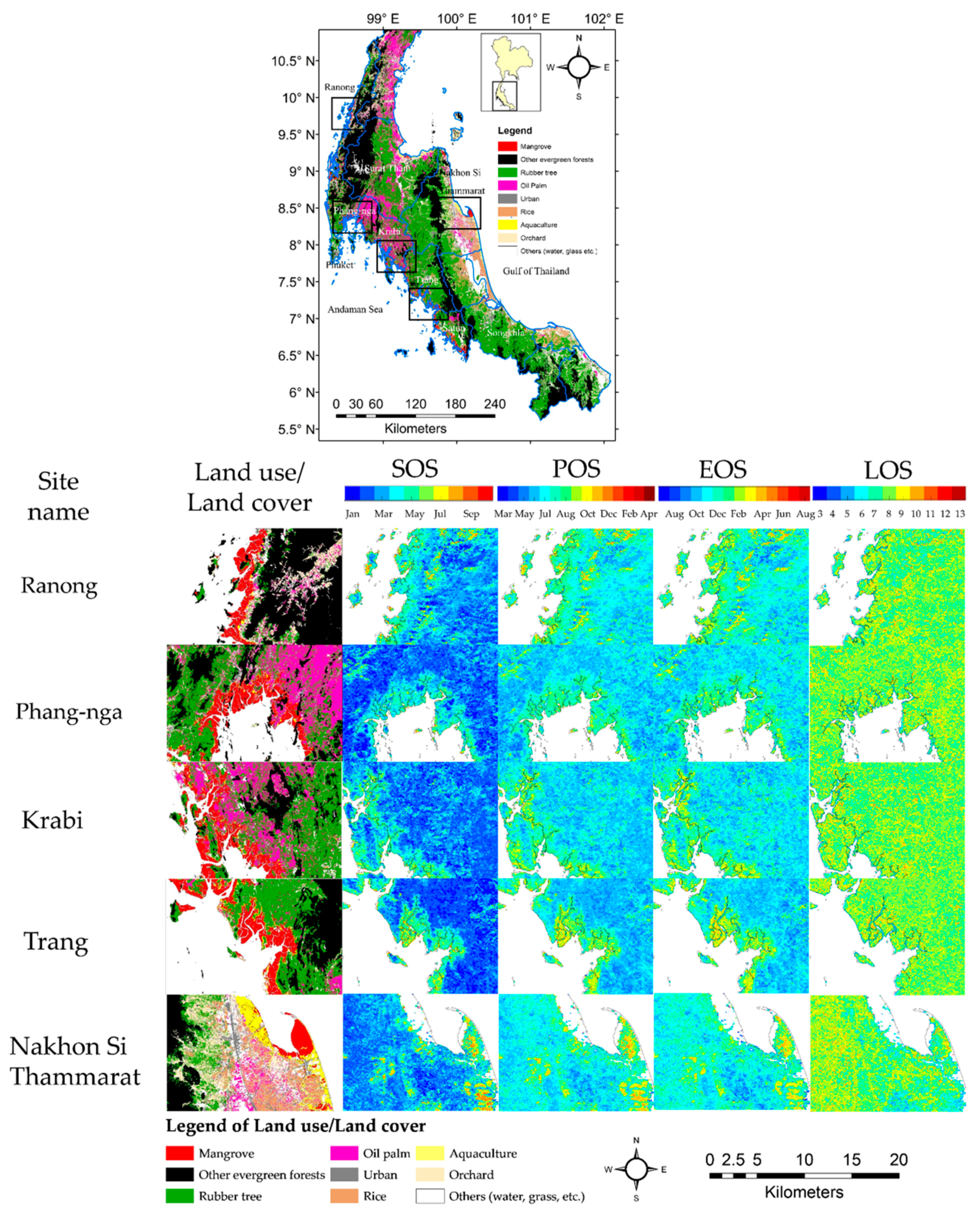
The Land Development Department of Thailand (http://sql.ldd.go.th/ldddata/) in 2012 mapped the mangrove areas in Thailand, which were mainly distributed over the south and east of Thailand. The largest areas of mangrove are in Southern Thailand (about 84% of the total mangrove area of Thailand, 2,235 km2 in 2012) while Rubber tree, Tropical rainforest, Oil palm, and Orchards are the major land use/land cover areas in Southern Thailand, accounting for 36%, 28%, 10%, and 6%, respectively. The mangrove area of Southern Thailand is around 1880 km2 (≈ 3% of land area). The study areas used here involved the mangrove forests along the southern coast of Thailand. The study sites with land use/land cover type are shown in Figure 1. Our study sites were located over a narrow range of latitudes. A mountain chain separated the four study areas on the Andaman Sea from the one study site on the Gulf of Thailand. This resulted in large differences in the timing of monsoonal rains between the western and eastern shorelines of the peninsula. Most of the upland tropical evergreen forests are distributed on a mountain chain that runs North–South along the Malay Peninsula.
The five study areas selected for this study (Figure 1) include: (1) Ranong province, (2) Phang-nga province, (3) Krabi province, (4) Trang province, and (5) Nakhon Si Thammarat province. The characteristics of the five selected sites are shown in Table 1. Ranong province site was declared to be a World Biosphere Reserve in 1977 by UNESCO and the Thailand Government [86,87]. This site is protected by the Thai government and known as Lamson National Park [88]. Phang-nga province site is located at Phang-nga Bay National Park covering the mangrove areas of Phang-nga province and a part of the mangrove area of Krabi province. This mangrove area is a dense healthy primary mangrove forest area. It is also an important Ramsar-listed wetland site in Thailand [87]. The bay is relatively shallow (around 1–4 m) with tidal amplitude between 1–3 m. This area is close to the high mountain areas in Myanmar (Burma) and Ranong and Phuket provinces of Thailand which are the source of several rivers that flow into Phang-nga Bay. Krabi and Trang province sites are other Ramsar-listed sites located in the Lanta National Park in Krabi province and the Palian-Langoo mangrove area in Trang and Satun provinces [87]. The mangrove area at Trang province site is composed of primary and secondary growth mangrove forest within six large river estuaries. The coast has a concave shape, with some narrow mud flats and sandy beaches. Mangrove forests at Trang province site experience a relatively high tidal amplitude and the tidal range also depends on the seasons. The last site, Nakhon Si Thammarat province, is located in the Gulf of Thailand on a cape extending into the sea. This mangrove area is the largest area on the South-East Coast of Thailand [87]. The Pak Phanang River is the main river in this area and its estuary is heavily charged with sediment. The dominant mangrove species and their relative abundances at Pak Phanang estuary area (Nakhon Si Thammarat province) are difference from the other sites [89] (Table 1).
The weather of Southern Thailand has two seasons, wet and dry season, with the wet season longer than the dry season. Regionally, the wet season approximately starts in June and finishes in January of the following year. The dry season usually starts in February and finishes around May of the same year. However, the monsoons of the Andaman Sea and the Gulf of Thailand are different in detail. The area on the West Coast on the Andaman Sea is affected by a West-South monsoon around May to October whereas the area in the Gulf of Thailand is affected by a North-East monsoon around September to December. The timing of the wet and dry season of the two coasts hence varies considerably. The climate of each study site species are shown in Table 1. The Ranong province site has the heaviest rainfall with a maximum of more than 4000 mm/year and Krabi province site has the least rainfall of about 1700 mm/year.
To validate the satellite data, a phenocam at Bangrong Bay, Phuket Province Thailand (the red point in Figure 1) was setup to monitor mangrove seasonality. This site is the biggest mangrove area in Phuket province (about 3 km2). The dominant species is Rhizophora apiculata. The camera was mounted on a mangrove tower at 8.051724 °N and 98.415384 °E (Figure 1). The height of the camera was about five meters above mean sea level and the field of view of the camera was oriented westwards (Figure 2). The observation periods were from March 2015 to August 2016. The camera captured images every 30 min [90,91] from 07:00 to 16:30 (local time). The focus length of the camera was set to infinity.
2.2. Data Used
2.1.1. Vegetation Index
The vegetation indices used to monitor vegetation phenology based on remote sensing are the Enhanced Vegetation Index (EVI) [20,43,65,100] and Normalized Difference Vegetation Index (NDVI) [19,35,66,67]. This study used EVI from the Moderate Resolution Imaging Spectroradiometer (MODIS). The EVI was designed to reduce atmospheric and soil background effects [101] and help reduce noise from cloud or atmosphere in tropical zones [20,32]. MODIS satellite images were downloaded from USGS (United States Geological Survey) available on https://earthexplorer.usgs.gov/. The 16-day composited EVI data was extracted from Terra-MODIS vegetation index product, MOD13Q1 at 250 m resolution (h27v08), from January 2002 to December 2014. The MODIS data were re-projected from Sinusoidal projection to Geographic projection, WGS 1984. The MOD13Q1 is widely used for assessing vegetation phenology e.g. [28,32,40,62,71,78,81,100,102]. In order to calculate vegetation index from the phenocam imagery, the Normalized Green-Red Difference Index (NGRDI = (DNG − DNR)/(DNG + DNR), [103]) was computed from the split Red, Green, and Blue phenocam images. All images from the camera were selected to correspond to the same time (around 10.30 AM at the local time) of the MODIS images. The NGRDI of all pixels in the ROI (Figure 2) of each image were calculated and then spatially averaged to the daily data. The daily data was averaged to monthly data to compare with MODIS EVI seasonality.
2.1.2. Mangrove Phenology Drivers
Monthly time series data of potential climate/aquatic drivers of mangrove phenology growth were obtained over the period from 2003 to 2012 and included air temperature (Ta), surface temperature (Ts), sea surface temperature (SST), rainfall, sea surface salinity (SSS), and radiation flux (Ra). Rainfall data was derived from the Tropical Rainfall Measuring Mission (TRMM-3B43) 0.25° x 0.25° spatial resolution, downloaded from http://mirador.gsfc.nasa.gov. The TRMM-3B43 is the monthly rainfall estimated by combining the 3-hourly merged high quality infrared estimates with the monthly accumulated rainfall from the Global Precipitation Climatology Centre rain gauge analysis [104] and specifically for Thailand [32]. The three drivers, Ta, Ts, and Ra are monthly data from the Global Land Data Assimilation System 2 (GLDAS-2) products which are publicly available data from NASA [105], at 0.25° spatial resolution, downloaded from https://hydro1.gesdisc.eosdis.nasa.gov/data/GLDAS. They calculated Ta from the atmospheric parameter models [106]. Ra used in this study is downward short wave radiation flux [23] represented as average monthly data calculated using the National Centers for Environmental Prediction (NCEP) model [106]. Monthly SSS was downloaded from Argo (http://www.argo.ucsd.edu). Argo is the globally estimated monthly data from the interpolation of measurement fields with 0.5° x 0.5° resolution [107,108]. Monthly SST is derived from MODIS-Aqua, at 4 km spatial resolution. SST data is estimated from band 31 (10.78–11.28 µm) and band 32 (11.77–12.27 µm), adjusted to sea surface temperature by comparison with in situ temperature [109]. SST was downloaded from NASA (ftp://podaac-ftp.jpl.nasa.gov/allData/modis/L3/aqua/11um/v2014.0/4km/).
2.3. Phenology Parameters Extraction
TIMESAT time-series analysis software [110] was used to extract mangrove phenological parameters. TIMESAT is software which is widely used to extract metrics of vegetation dynamics [27,75,77,82]. To minimize the effect of cloud cover and other noise sources, common in tropical areas [111], a Savitsky-Golay (SG) smoothing filter was applied to the MODIS-EVI time series [29,32,71,77,112]. The EVI from the resulting smoothed data was used to calculate the phenological parameters. Four parameters were retrieved: (1) Start of the season (SOS) defined as the time at which the EVI value was 20% [29,32,62,81] of the distance between the prior minimum EVI and peak EVI level, (2) End of the season (EOS) defined as the time at which the EVI was 20% of the EVI value between the post season minimum and peak EVI level (same criterion as was used for SOS above), (3) Peak of the season (POS) is the time at which maximum EVI value is reached, between SOS and EOS, i.e., the vegetation has maximum productivity [113], (4) Length of the season (LOS) is the difference, in months, between SOS and EOS [29,77]. A 3-year EVI time-series was used to calculate the phenological characteristics, e.g., to extract the phenology metrics for 2007, the images in years 2006, 2007, and 2008 were needed. So, 13 years of EVI data (2002 to 2014) were used to retrieve 10 years (2003 to 2012) of the phenological characteristics of the mangroves sites in this research.
2.4. Analysis
Mangrove phenology analyses were separated into within site and cross site analyses so that the differences in the relative weight of the various possible control factors could be distinguished from differences due to site location and species composition. Because there were differences in the spatial resolution between EVI and drivers, the pixel of each driver that covered each of the mangrove areas was extracted and averaged into monthly data.
2.4.1. Mangrove Phenology Characteristics
The seasonal mangrove data were converted from 16 day EVI to monthly EVI and averaged over 10 years (2003 to 2012). To compare differences of mangrove phenology at each study site, boxplot methods were applied.
2.4.2. Comparisons between Mangrove Phenology with Surrounding Land-Based Tropical Forests
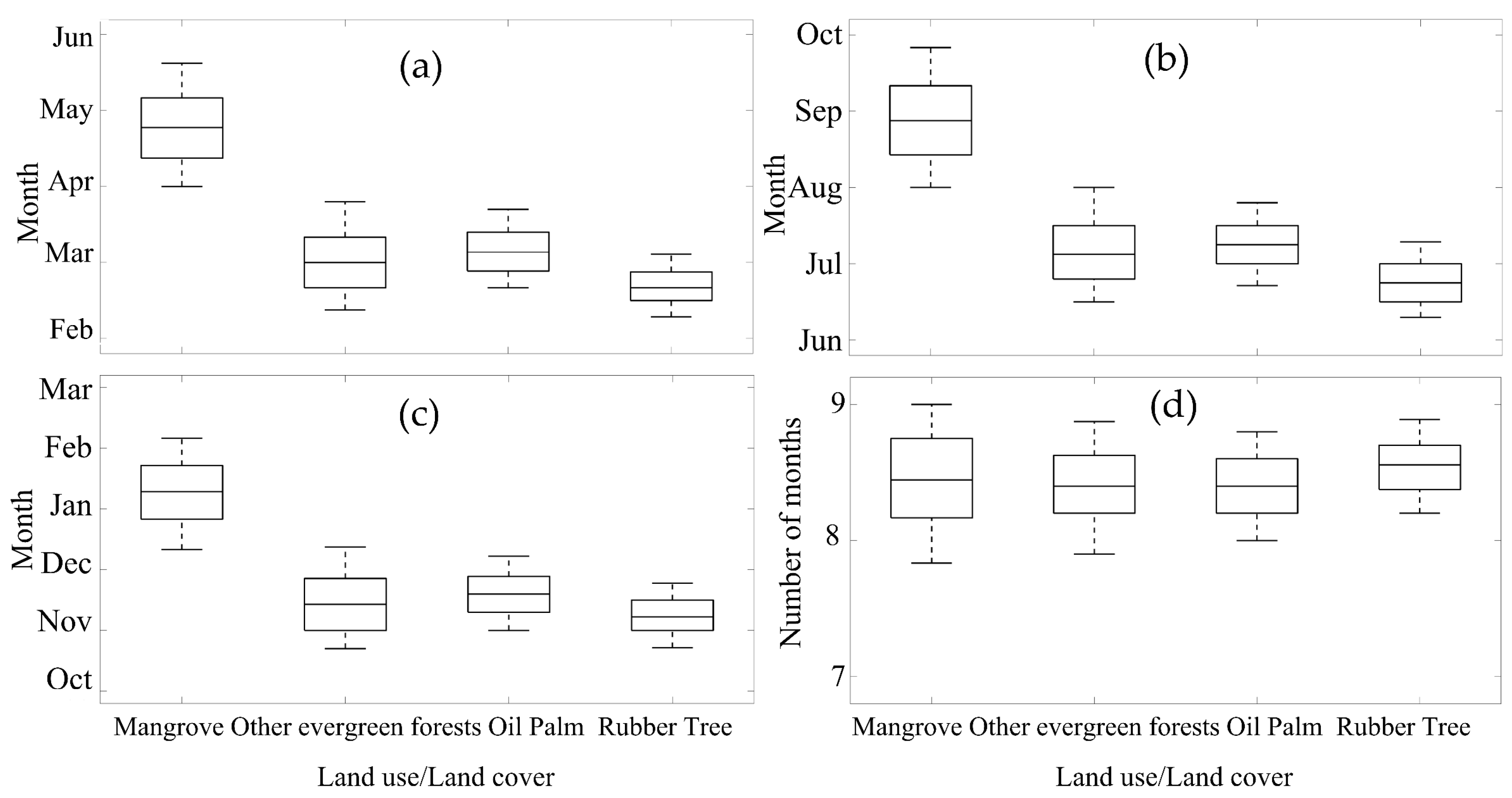
The three land-based evergreen forests used for comparison in this study were (1) Rubber tree plantations, (2) Oil palm plantations, and (3) Other evergreen forests which are the main land cover types of southern Thailand. All pixels of each of the phenology parameters of each of the land cover types in southern Thailand were extracted and presented as boxplots for further analysis of the differences between mangrove phenology with the surrounding land-based tropical forests.
2.4.3. Identification of the Drivers of Mangrove Phenology
We used climate and environmental data for 2003–2012 (10 years) and EVI data for 2002–2014 (13 years). We used the monthly data (both climate and environmental and EVI data) over 10 years (2003 to 2012 or 120 months) to calculate correlation coefficients between EVI and the climate/aquatic drivers (rainfall, Ta, Ts, SST, Ra, and SSS) on a site by site basis. Lag analysis was also applied with the lag month as the difference (in months) between EVI and the drivers which maximized the correlation (r2) between EVI and the driver. We selected four conditions for month lag analysis: (1) 3-months lag before, (2) 2-months lag before, (3) 1-month lag before, and 4) the same month (lag = 0). For example, the lag of 3-months before means that if the driver data is in January, the EVI effect will be observed in April; or if the driver data is in March, the EVI effect will be observed in June. The best coefficient of determination (r2) was selected to explain the relationship between EVI and climate/aquatic drivers. The maximum correlation coefficient and the optimum month lag are reported.
Second, to identify the drivers of the phenology patterns and shifts, we conducted site by site analysis. Previous studies used fixed lag-times rather than estimating it statistically as the present study: Pastor-Guzman et al. [84] used the cumulative rainfall from January to March for every year during 2009 to 2011 while Liu et al. [34] used mean temperature and cumulative rainfall in spring (March to May) or winter (December to February) to analyze the green-up date shift for every year during 1999 to 2013. In this study, we used the average phenology parameters (calculated from all pixels for each study site) of each year as the selected month for extraction the Ta, Ts, SST, SSS, Ra, and rainfall driver data. The lag analysis condition between phenology parameters and their drivers are the same as the EVI and climate/aquatic drivers including the selection of the best correlation coefficient and optimum month lag.
Third, the trend of phenology parameters from 2003 to 2012 was analyzed using the slopes of linear regressions [34]. The phenology parameters of each year were averaged over the mangrove area of each site.
3. Results
3.1. Seasonal Profiles and Phenology of Mangrove Sites
The EVI seasonal profiles of different land cover and land use types are shown in Figure 3. The land cover types included the mangrove forest of each site, other evergreen forest, rubber tree and oil palm where the last three types are the most common land cover in southern Thailand. The figure shows whether or not there is a different pattern for all the land cover land use types including the mangrove forest. Special attention was paid to the peak of season which is different for the four types of forest.
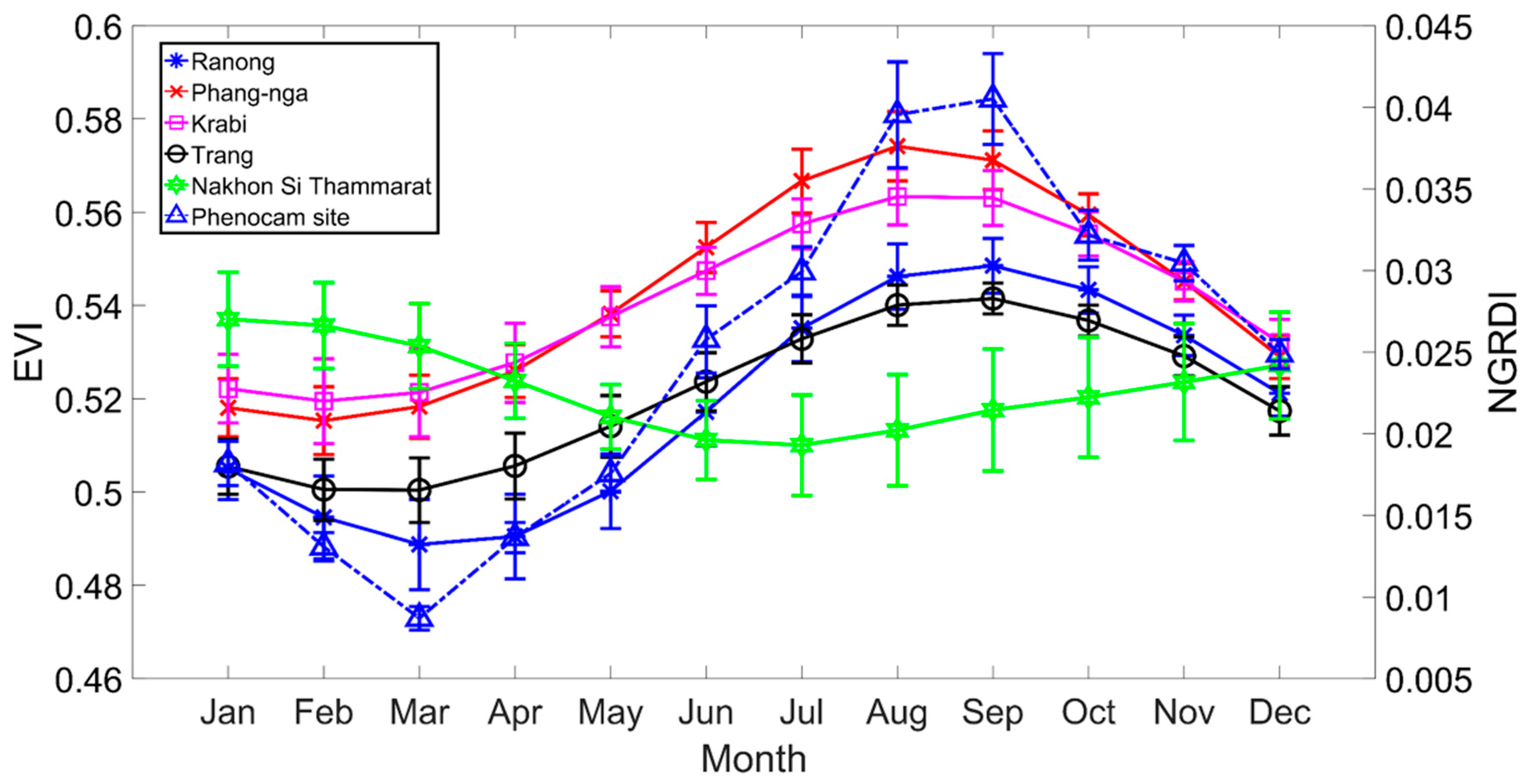
The average monthly EVI seasonal profile at each study site using all mangrove pixels over the 13 years (2002–2014) of EVI data analyzed in this study and averaged monthly NGDRI from phenocam over March 2015 to August 2016 is shown in the Figure 4. The EVI values were mostly between 0.5–0.6 and exhibited strong seasonality at all sites. The seasonal profile of Ranong and Trang province site were similar, with the minimum EVI in February/March and increasing to maximum values in August and then decreasing to a minimum again in the dry season of the following calendar year. The seasonal profiles of Phang-nga and Krabi province site were also similar, with the minimum EVI in February and increasing to a maximum EVI in September. On the other hand, the seasonal profile of Nakhon Si Thammarat province site (on the other side of the peninsula) shows a minimum EVI in July, increasing to a maximum in January of following year. The phenocam color index, NGRDI also exhibited strong seasonality. The seasonal characteristics of this index start with a minimum in March and increase to maximum values in September. Overall, the EVI seasonal profiles at the four Andaman Sea sites from MODIS were similar to the NGRDI from the phenocam data, which was also located at an Andaman Sea site.
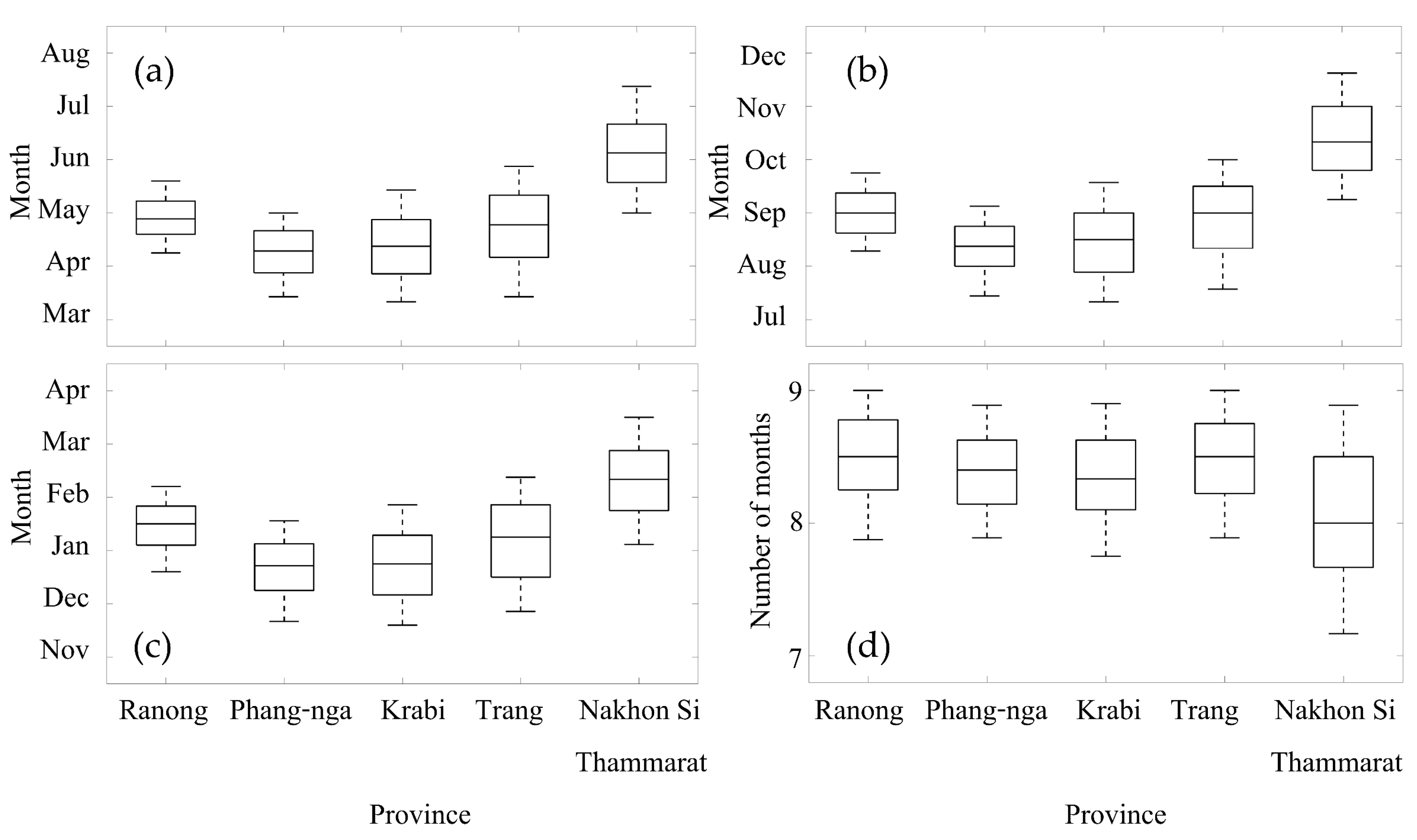
Figure 5 shows TIMESAT derived phenology parameters (SOS, POS, EOS, and LOS) map averaged over the ten years at each of the study sites and the boxplots of phenology metrics are shown in Figure 6. The SOS of Phang-nga and Krabi province sites occurred around April, with SOS of Ranong and Trang province sites occurring one month later, around May, while the SOS of Nakhon Si Thammarat province site was found to be much later, around July. The POS of Phang-nga and Krabi province sites were in August, with POS of Ranong and Trang province sites one month later in September, whereas the POS of Nakhon Si Thammrat province site was not until November. The EOS timings of Phang-nga and Krabi, Ranong and Trang, and Nakhon Si Thammarat province sites were in the subsequent years around January, February, and March, respectively. The averaged LOS for all sites remained the same at approximately 8–9 months. Overall, the phenology Phang-nga and Krabi province sites started earlier than the phenology of site of Ranong and Trang province site, while the temporal cycle of Nakhon Si Thammarat province site was the latest of all five sites. In conclusion, the SOS of all Andaman Sea mangrove sites (west coast) started in April–June, with peaks in August–October and end of the growing season in January–February of the following year, with the length of season about 8 months. For the mangrove phenology at the Gulf of Thailand site (east coast), the SOS started in July, with peaks in November and with an end of the season in March of the following year. The average of length of season of the mangrove at the Gulf of Thailand was similar to the Andaman Sea sites but with a different standard deviation. However, it seems the EVI profile at Nakhon Si Thammarat site (Figure 4a) was quite different compared to the west coast sites and the phenology parameters (especially POS) also were markedly different (Figure 6). If we consider the species contribution (Table 1), we found that there are many mangrove species in the Nakhon Si Thammarat site that are not found in the west coast sites. Averaging EVI for sites with mixed stands of several species may have caused differences in EVI profiles.
3.2. Comparison of Mangrove Phenology with Surrouding Land-Based Tropical Forests
The three main upland land cover types surrounding the mangrove study sites included other evergreen tropical forests and converted oil palm and rubber tree plantations. The spatial variability (Figure 5) and boxplots (Figure 7) of the mangrove phenology metrics show the mangrove areas to have distinct phenology patterns that are clearly separated from the phenology patterns of the surrounding upland land cover types areas (Figure 3 and Figure 5). These results show that the MODIS EVI profiles can be used to separate the phenology of mangroves from terrestrial vegetation. Overall, the mangrove phenologies were shifted to later in the year by approximately 2 months compared with the land-based tropical forests. However, the averaged length of the growing season of the mangroves was quite similar to the land tropical forest, at about 8 months duration.
3.3. Mangroves Phenology Drivers
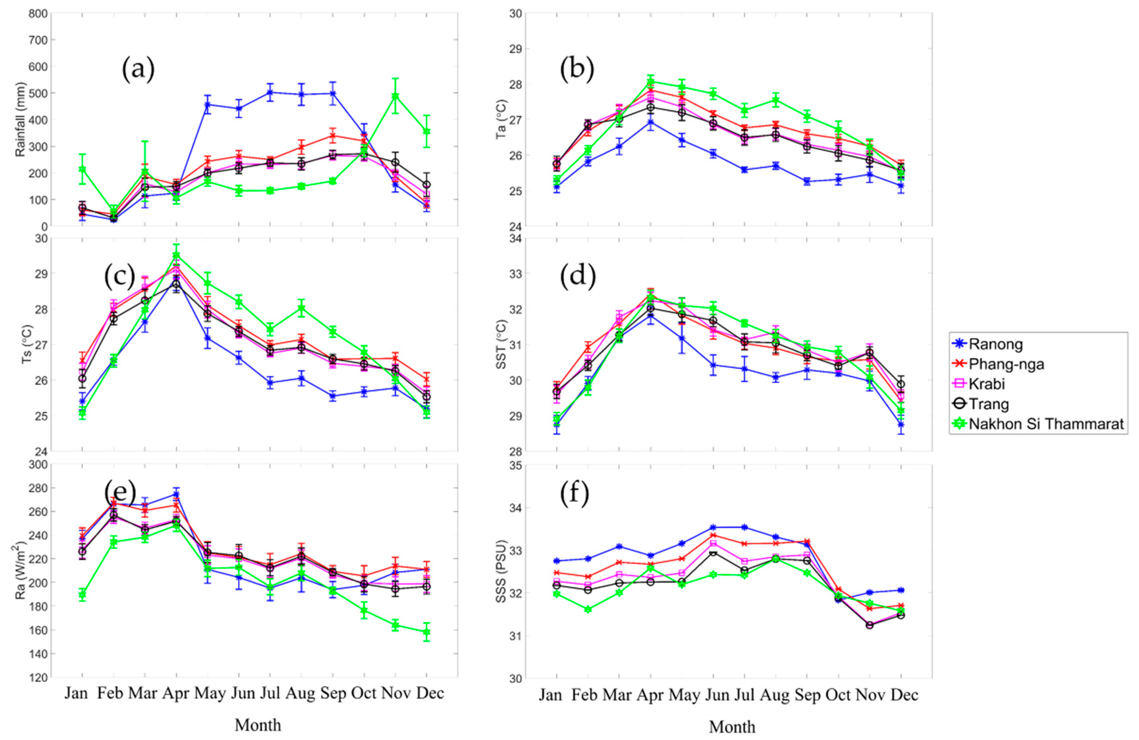
Six environmental and climate drivers: rainfall, air temperature (Ta), surface temperature (Ts), sea surface temperature (SST), radiation flux (Ra), and sea surface salinity (SSS) were used to analyze relationships with the mangrove growth phenology metrics over the 10-year period, 2003–2012 where we had climate data. Each of the drivers showed similar seasonal patterns (Figure 8) for all sites, except for seasonal rainfall magnitudes, which were different between the Andaman Sea sites (Ranong, Phang-nga, Krabi and Trang province sites) and the Gulf of Thailand site at Nakhon Si Thammarat province. The maximum rainfall (Figure 8a) of Ranong, Phang-nga, Krabi and Trang province sites were in September whereas the rainfall maximum at Nakhon Si Thammarat site was in November. The Ta, Ts, and SST (Figure 8b, Figure 8c, and Figure 8d) and also Ra (Figure 8e) all have maxima in April. The SSS (Figure 8f) shows the same pattern for all sites with a maximum in June/August.
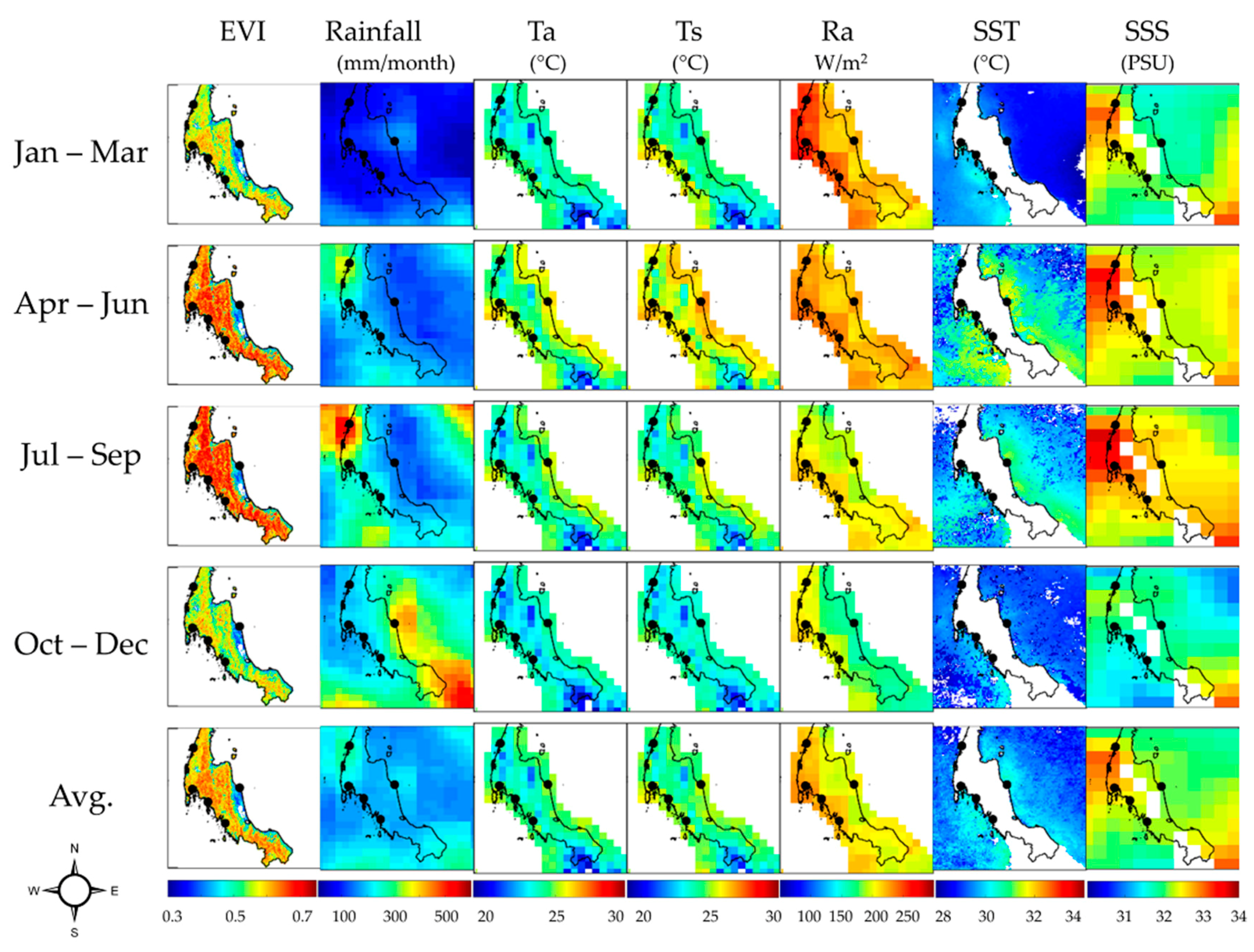
Figure 9 shows the spatial variability of seasonal EVI and environment/climate drivers at quarterly intervals. The difference in the timing of the maximum seasonal rainfall between Andaman Sea and Gulf of Thailand was about 2 months (Figure 8a and Figure 9). However, the minimum rainfall was in February for all sites. The rainfall at Ranong province site was higher than the other sites from April to October.
In addition, the seasonality of EVI (Figure 4) was positively correlated with the seasonal rainfall pattern at both the Andaman Sea sites and the Gulf of Thailand site. The lagged EVI profile at the Nakhon Si Thammarat site, compare to the other site, corresponded to the lagged shift in rainfall seasonality at Nakhon Si Thammarat (Figure 8a), relative to rainfall seasonality at Andaman Sea sites, Furthermore, of the drivers examined in this study, only rainfall (magnitude and seasonality) showed a marked difference between Gulf of Thailand and Andaman Sea (Figure 8a).
The Figure 8 shows that the increase in temperature (Ta and Ts) and radiation flux signals at the start of leaf fall in mangrove (EOS) because while the temperature is increasing (Figure 8b, Figure 8c and Figure 8d), the EVI of the mangrove is decreasing to a minimum (Figure 4). On the other hand, when temperature and radiation fluxes decreased in April, this signaled the beginning of the rainy season (Figure 8a) and corresponded to the emergence of new mangroves leaf growth (SOS as shown in Figure 5).
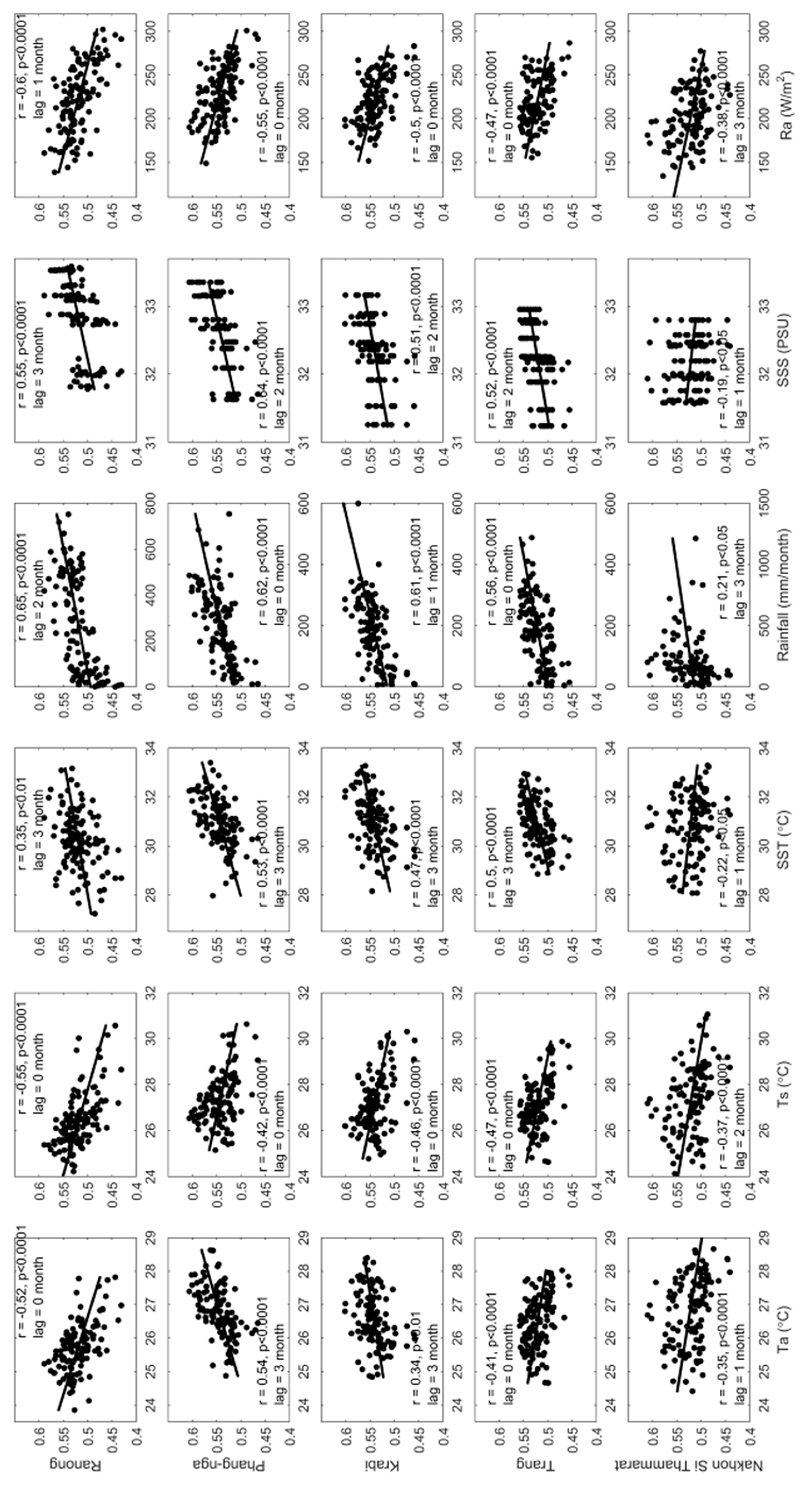
The correlations between EVI of mangroves and the climate/aquatic drivers are shown in Figure 10, which also shows the lag month relationships. From this figure, the Ts and Ra were negatively related for all sites. In contrast, only rainfall was positively related with EVI at all sites. In addition, not only Ta and SST but also SSS were sometimes negatively and sometimes positively related, such as Ta was positively related at the Phang-nga site but negatively related at the Krabi province site. Generally, higher SSS or SST will be inversely correlated with EVI. This research found this negative relation to be quite clear at Nakhon Si Thammarat (the site of in the Gulf of Thailand) but not as clear at the Andaman Sea sites. The reason may be that the effects of other drivers, such as rainfall, were dominant at these sites and shadowing, resulting from cloudiness, minimized mangrove saturation at very high irradiance conditions. The lag analysis between EVI and the drivers (Figure 10) show whether EVI of mangrove responded to the driver immediately or not. There is some evidence for lagging especially for SST and SSS and even rainfall at the Ranong province site. The maximum lag for Ta was 3 months at Phang-nga province site, the Ts lag was 2 months at Nakhon Si Thammarat province site, the lag for SST was 3 months at Ranong, Phang-nga, Krabi, and Trang province sites, the lag for rainfall effects was 3 months at Nakhon Si Thammarat province site, the lag for SSS was 3 months at Ranong province site and the lag for Ra was 2 months at the Nakhon Si Thammarat province site.
The relationship between mangrove phenology metrics and drivers was analyzed (Figure S1 in supplementary data). The results indicated that the cumulative rainfall was likely to be the main factor driving green-up date (SOS) with later dates observed at Ranong (r = +0.74, p < 0.05) and Phang-nga (r = +0.75, p < 0.05) sites. Increasing rainfall about three months (lag = 3 months) before the SOS induced later SOS. Ta is another important driver for POS where it is significant (p < 0.05) for all sites at both the Andaman Sea and the Gulf of Thailand. However, increasing averaged Ta over the previous time of about 2 months beforehand results in a later POS on the Andaman Sea sites but it is earlier at the Gulf of Thailand sites. SST is a driver for EOS which shows a positive relation (p < 0.05) for both the Andaman Sea (Ranong and Trang province) and the Gulf of Thailand (Nakhon Si Thammarat). However, the increasing of SST caused a later EOS by only about 0–1 month.
3.4. Trend Analysis
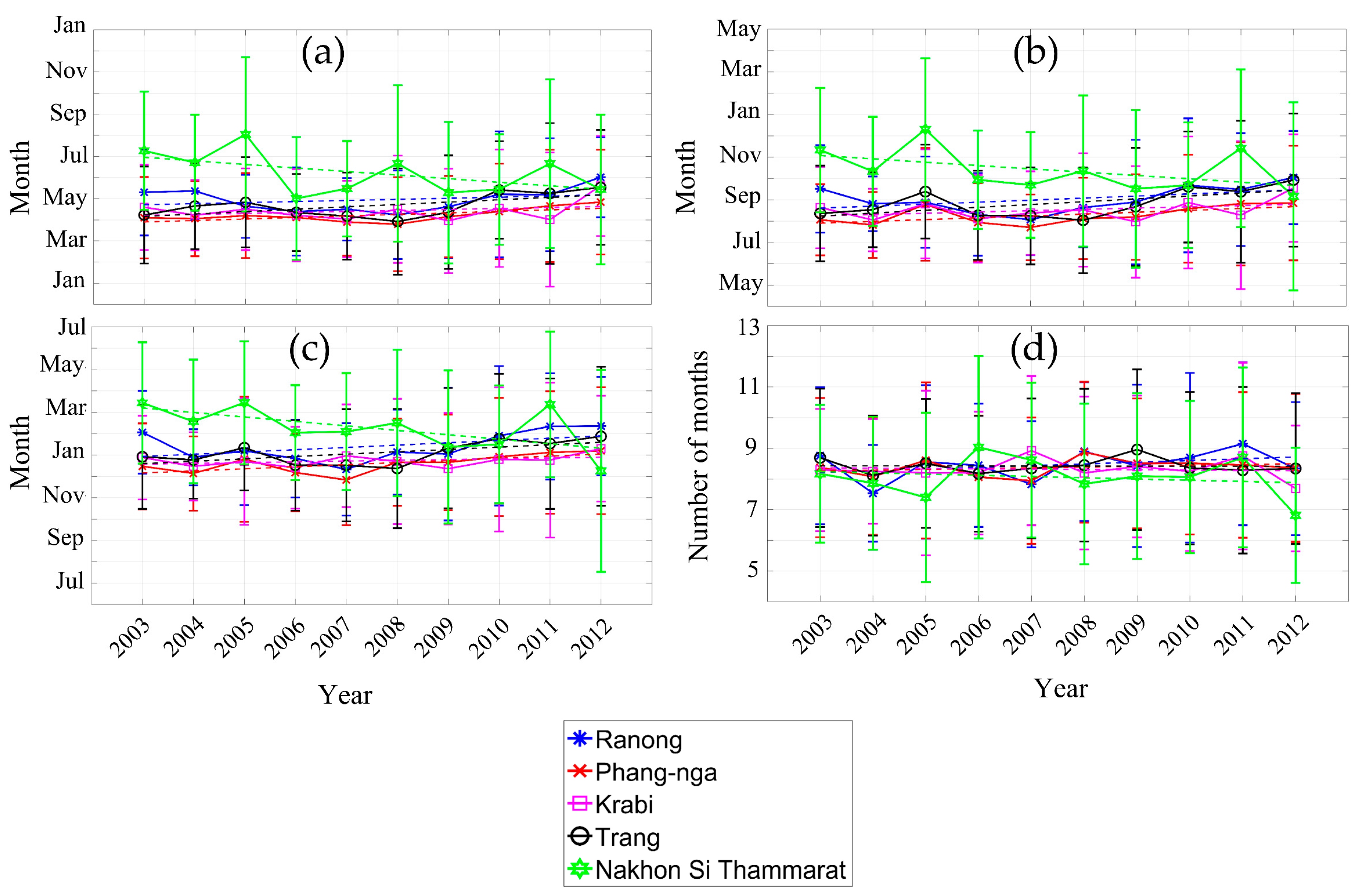
Figure 11 illustrates the inter-annual variability of mangrove phenology during 2003–2012 over the five study sites. Table 2 shows the slope of the linear fitted equations of phenology parameter vs. time. The positive slope indicated a delayed mangrove phenology and a negative slope indicated an advanced phenology or an earlier onset of mangrove growth. A delayed trend of SOS was observed at Phang-nga province site with slope of +0.072 month/year (R2 = 0.446, p < 0.05). The delayed trend of SOS at Phang-nga province site would be expected to result in a delayed POS trend (+0.086 month/year, R2 = 0.359, p < 0.1) and delayed EOS trend (+0.098 month/year, R2 = 0.450, p < 0.05). EOS significantly advanced at Nakhon Si Thammarat province site (–0.209 month/year, R2 = 0.373, p < 0.1). There was no statistical trend of LOS vs. time, for all sites through the ten years of this study.
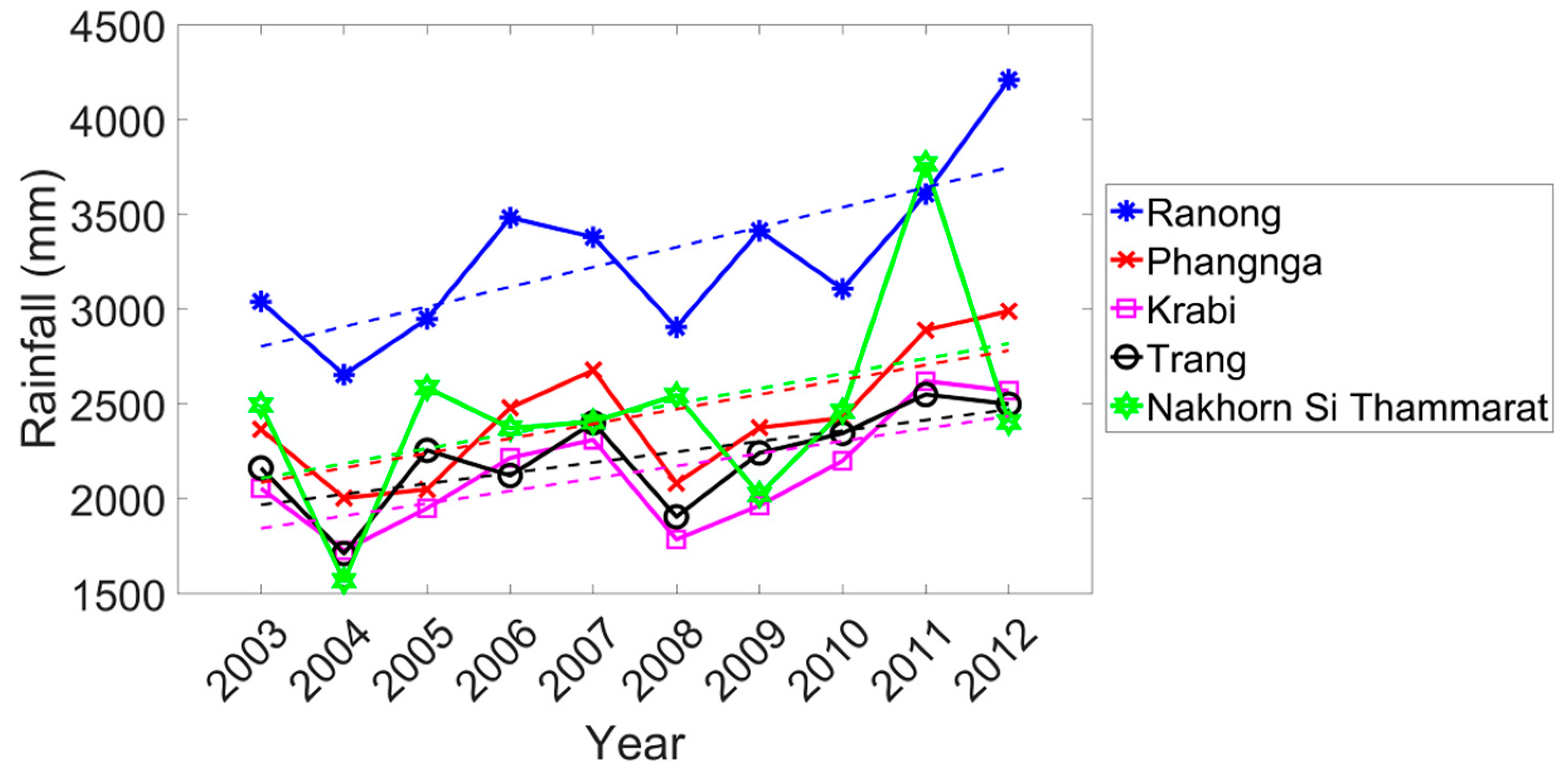
Figure A1 shows the trend of rainfall over ten years. Overall, the rainfall has a positive trend for all sites where the Ranong province site had the most positive trend (+104.971 mm/year, R2 = 0.513, p < 0.05) and the lowest trend was in the Trang province site (+55.821 mm/year, R2 = 0.423 p < 0.05), while the trend of rainfall at Nakhon Si Thammarat province site was not significant. However, the significant positive trend of rainfall at Phang-nga province site may induce a significant delayed trend of phenology for this site including Trang province site.
4. Discussion
This study is the first satellite-based mangrove phenology analysis with climate and aquatic environment drivers in Thailand. The study was conducted on the Malay Peninsula which is vital to the Indo-Malay region of biodiversity. The existing literature on mangrove phenology in Thailand encompasses a few decades [114,115,116], but was mainly based on field survey techniques. The SOS results found in the present study agree with those of Wium-Andersen [116] who reported that the appearance of new leaves of Rhizophora apiculata are maximal in May–June.
Our results demonstrated that the EVI derived from MODIS satellite data could be used to retrieve mangrove phenology parameters (Figure 4) similar to other studies conducted in tropical forests [20,84,117]. Although MODIS has been less successful in retrieving phenology over evergreen forests [83], we found clear mangrove phenologies in Southern Thailand with SOS, POS and EOS in April – June, August–October and subsequent year January–February, respectively (Figure 5). The SOS occurred before pre-monsoon, POS occurred during the monsoon and EOS occurred post-monsoon, which corresponded to maximum litter fall period of tropical mangroves in India [118], corresponding to the study of Pastor-Guzman et al. [84] who reported the SOS and EOS of mangroves at Yucatan Peninsula coastline, Mexico was related with rainfall seasonality, with SOS occurring from late dry season to the rainy season and EOS occurring from mid-dry season to late rainy season. The LOS of mangroves at our study sites was found to be about 8–9 months. Previous studies have shown that the length of the growth season in mangrove forest [84] and other tropical rainforest [119,120] is about 8–12 months.
Mangrove phenology derived from MODIS data could also discriminate mangrove phenology from that of surrounding land-based forests (other evergreen forests, oil palm, and rubber tree plantations) (see Figure 3 or Figure 4). Kou et al. [117] also reported that they could distinguish different types of tropical evergreen forests in mountainous regions. The seasonality of the EVI of tropical mangroves in our study had a positive correlation with rainfall (Figure 8, Figure 9 and Figure A1) which agrees with the findings of Suepa et al. [32] who reported that the tropical forest was regulated by rainfall magnitude and seasonality. In addition, the large differences of rainfall period between the Andaman Sea and Gulf of Thailand sites resulted in differences in the temporal cycle of EVI at the two coastlines (Figure 4). Over the course of the study, there were significant increases in rainfall on the Andaman Coast but not at the Gulf of Thailand site. The inverse relationship between the EVI of mangroves with surface temperature (Ts) (Figure 10) reflected stressful high temperature effects that decreased leaf production [121]. According to results reported by Clinton et al. [63] and Prasad et al. [119] there was no significant correlation of EVI with SST due to significant lags in vegetation responses. This study confirmed the EVI response of mangrove lagged SST of about 1 to 3 months. As mangroves were most strongly related with rainfall seasonality, radiation flux (Ra) was inversely related to EVI seasonality, although there may also have been photo inhibitive effects of high irradiances in mangroves, which are considered “sun plants” with typically very high irradiances point [122,123,124].
This study showed the timing relationships between mangrove phenology metrics and climate/aquatic drivers and also presented a lag month analysis with a new novel method. The results confirmed that the drivers had lag month relations with mangrove phenology. Rainfall was the main driver (p < 0.05), especially for SOS. We found that high cumulative rainfall resulted in a later SOS, as the SOS of the mangroves was in the pre-monsoon period. Ta (air temperature) was significant for only POS at all sites but this driver’s impact on mangrove phenology was complicated because it made for an earlier phenological response at one site (Gulf of Thailand, Nakhon Si Thammarat) while the other sites (Andaman Sea sites) had much greater lags. The results of this study corresponded with findings of Liu et al. [34] who reported the green-up of grassland in China was earlier with increasing temperature, while Pastor-Guzman et al. [84] showed earlier mangrove phenology shifts (SOS and POS) with rainfall increases.
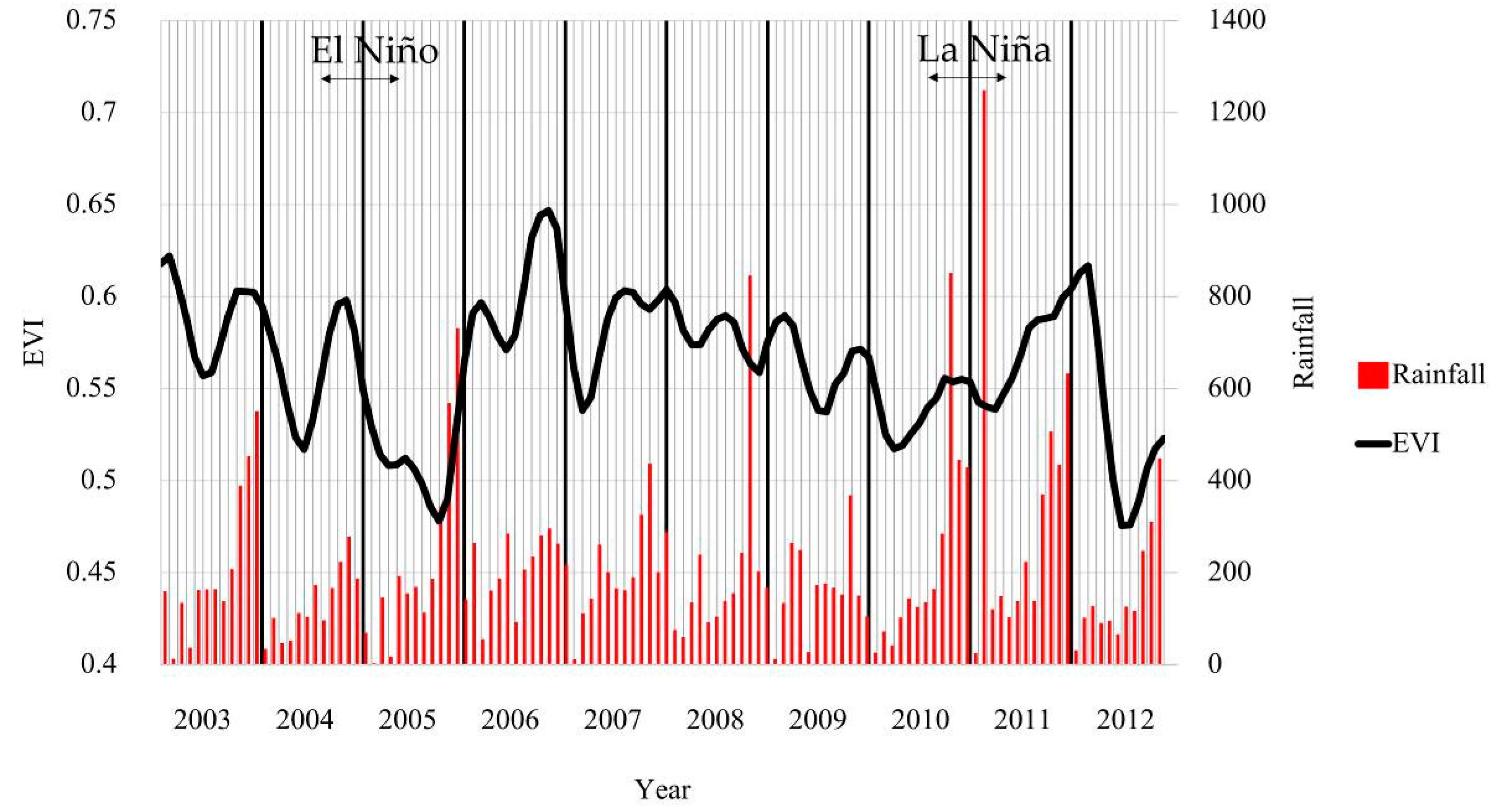
As the EVI of each month oscillates (Figure 4), one of the manifestations of this is the observed changes in the standard deviation of each month. The highest standard deviation was during the wet season at site Nakhon Si Thammarat and during the dry season at Ranong and Krabi province sites. These oscillations of EVI were a function of environmental drivers such as rainfall and temperature (Figure 10). The dominant mangrove species in each particular site was a factor that caused different EVI values, especially at Nakhon Si Thammarat province site, where there were much more species that were averaged. In addition, the El Niño (drier than normal) and La Niña (wetter than normal) years influenced mangrove phenology, especially SOS, POS, and EOS at Nakhon Si Thammarat province site (see Figure 9 and Figure 12). The EOS in 2004 occurred around March and the SOS in 2005 was delayed to August, while generally, SOS occurred around June/July. This delay of SOS may be a manifestation of the effects of El Niño in 2005 [125], as there might not have been enough fresh water flow into the mangrove forests resulting in higher salinity and causing increased stress on the mangroves [18]. However, the stress on the mangroves decreased because there was high rainfall (more than 200 mm/month) from March 2006 to the end of that year (Figure 12). The start of season (SOS) in 2006 was therefore what would be expected during a “typical” year (Figure 11). The La Niña phenomena at the end of 2010 to April of 2011 (see Figure 12) resulted in a later EOS at Nakhon Si Thammarat province site in April, where it generally occurred in February. In contrast, there was low rainfall after the La Niña phenomena but there was a normal SOS of mangrove in 2011. However, the high rainfall events at the end of 2011 (Figure 12) at Nakhon Si Thammarat province site accounted for the fluctuation of the EOS at that site (Figure 11).
This study not only assessed mangrove phenology, but also phenology trends were analyzed. There was a significant increase in rainfall on the Andaman coast but not at the Gulf Coast site over the course of this study (Appendix A). Our results indicated a significant later phenology (see Table 2) at Phang-nga province site (p < 0.05) and Trang province site (p < 0.1), both of which are on the Andaman Sea site but the largest contrast was at Nakhon Si Thammarat province site located on the Gulf of Thailand compared to the Andaman Sea sites. Differences in mangrove phenology trends between the east and west coasts of Southern Thailand may reflect the rainfall amounts and timing due to the mountain range separating the west coast sites from the east coast site (Figure 1). Krauss et al. [126] accounted for differences in the growth rate of mangroves in terms of hydro geomorphic zones. Rainfall on the Andaman Sea coast was not only higher than that for the Gulf of Thailand (Figure 8a and Figure 9) but has a different temporal pattern. Not only does rainfall affect shifts in phenology but also the stress of high temperature on vegetation are known to shift phenological responses [35,121,127]. Previous studies in temperate climates show that an increase of temperature of about one degree could result in an earlier SOS by about 4.2 days at a China site [34] and 5 days for fruit trees in Germany [39].
5. Conclusions
The phenology of mangrove forest in Southern Thailand was assessed with MODIS EVI at 250 m resolution over four sites on the Andaman Sea and one site on the other side in the Malay Peninsula facing the Gulf of Thailand. Our results demonstrated that MODIS images distinguished mangrove phenology from surrounding land-based tropical evergreen forest, oil palm, and rubber tree plantations phenologies. Although, the average lengths of the growing season (LOS) for all land cover types were quite similar, this research found there were significant differences and shifts in all other phenology metrics between each land cover type and the mangroves. Overall, the mangrove phenology metrics (SOS, POS, and EOS) lagged the surrounding tropical forests by about 2 months. The mangroves growing on the Andaman Sea side of Southern Thailand started greening in April to June and with peaks in August to October, and the end of season in January to February on the following year. The length of the growing season was about 8–9 months. However, the mangrove phenology at the Gulf of Thailand site had a distinctly different phase cycle than the mangrove phenology at the Andaman Sea sites. The growing season started about two months later in the Gulf of Thailand compared with the Andaman Sea sites. The differences in mangrove phenology trends between the east and west coasts of Southern Thailand reflected differences in the monsoon cycle and the mountain range running north–south along the peninsula. Rainfall was the only driver that showed a positive relationship for all sites while Ts and Ra showed negative relationships with EVI seasonal for all sites mangrove sites. Additionally, this research showed whether EVI of mangrove responds or not to the driver immediately. There is some evidence for lagging of about 0 to 3 months (0 is no lagging).
Rainfall significantly increased over the 10-year period at the Andaman Sea sites but not at the Gulf of Thailand site (Appendix A). There is a significant linear trend relation in the case of some phenology characteristics vs. time, for example, SOS (+0.072 months/year, R2 = 0.446, p < 0.05) and EOS (+0.098 months/year, R2 = 0.450, p < 0.05) at Phang-nga province site. The delayed SOS also induced a delay of POS (+0.086 months/year, R2 = 0.359, p < 0.1). EOS is significantly earlier at the Nakhon Sit Thammarat province site (–0.209 month/year, R2 = 0.373, p < 0.1) indicating an earlier end of the growing season. The El Niño (drier than normal) and La Niña (wetter than normal) also influenced the mangrove phenology later shift, especially SOS, POS, and EOS.
Supplementary Materials
The following are available online https://www.mdpi.com/2072-4292/11/8/955/s1, Figure S1: Scatterplots of the relationship between phenology parameters and drivers at five study sites: The Andaman Sea sites (Ranong, Phang-nga, Krabi and Trang), and the Gulf of Thailand site (Nakhon Si Thammarat). The lag month in the figure shows the lag-time in months (0, 1, 2, or 3) that gave the best correlation coefficient in the lag-time analyses. Lag-times were calculated using average monthly Ta, Ts, SST, SSS, and Ra: for example, if a parameter measured in May is a manifestation of a driver with a 3-months lag-time then the driver was the prevailing conditions 3 months before (in February). In the case of rainfall, the sum of the cumulative rainfall was used (0, 0 + 1, 0 + 1 + 2, and 0 + 1 + 2 + 3 months). For rainfall a lag time of 3 months reflects the cumulative rainfall over the previous 3 months, not just the monthly rainfall that occurred 3 months previously. Thus, a 3-month lag for the rainfall driver for the month of May reflects cumulative rainfall from Feb to May.
Author Contributions
A.H., W.K., V.S. designed the research. V.S., W.K., A.H., and R.J.R. contributed to the writing and commented on the manuscript from a Plant Biologist’s outlook.
Funding
The study was financed by faculty of Technology and Environment, Prince of Songkla University.
Acknowledgments
The authors would like to acknowledge the Faculty of Technology and Environment, Prince of Songkla University, Phuket campus, Thailand for providing financial support. The data used in this study were acquired as part of the mission of NASA’s Earth Science Division and archived and distributed by the Goddard Earth Sciences (GES) Data and Information Services Center (DISC), Physical Oceanography Distributed Active Archive Center (PO. DAAC), ARGO, NASA, USA.
Conflicts of Interest
The authors declare no conflict of interest.
Appendix A
Figure A1.
Accumulated annual rainfall of the five mangrove sites.


Table A1.
Statistics of accumulated annual rainfall trends.
| Site | Ranong | Phang-nga | Krabi | Trang | Nakhon Si Thammarat |
|---|---|---|---|---|---|
| Slope (mm/year) | 104.971 | 77.469 | 65.805 | 55.821 | 79.104 |
| R2 | 0.513** | 0.475** | 0.433** | 0.423** | 0.189 |
Note: ** p < 0.05.
References
- Alongi, D.M. Carbon sequestration in mangrove forests. Carbon Manag. 2012, 3, 313–322. [Google Scholar] [CrossRef]
- Food and Agriculture Organization of the United Nations (FAO). The World’s Mangroves 1980–2005; Food and Agriculture Organization of the United Nations (FAO): Rome, Italy, 2007. [Google Scholar]
- Suratman, M.N. Carbon Sequestration Potential of Mangroves in Southeast Asia. Manag. For. Ecosyst. Chall. Clim. Chang. 2008. [Google Scholar] [CrossRef]
- Pascual Serrano, D.; Vera Pasamontes, C.; Girón Moreno, R. The Energetics of Mangrove Forests; Springer: Queensland, Australia, 2009. [Google Scholar]
- Adeel, Z.; Pomeroy, R. Assessment and management of mangrove ecosystems in developing countries. Trees Struct. Funct. 2002, 16, 235–238. [Google Scholar] [CrossRef]
- Linneweber, V. Mangrove Ecosystems: Function and Management, 1st ed.; Springer: New York, NY, USA, 2002. [Google Scholar]
- Barbier, E.; Sathirathai, S. Shrimp Farming and Mangrove Loss in Thailand; Edward Elgar Publishing: Cheltenham, UK, 2004. [Google Scholar]
- McLeod, E.; Salm, R.V. Managing Mangroves for Resilience to Climate Change; World Conservation Union (IUCN): Gland, Switzerland, 2006. [Google Scholar]
- Hogarth, P.J. The Biology of Mangroves and Seagrasses; Oxford University Press: New York, NY, USA, 2007. [Google Scholar]
- Sitoe, A.A.; Júnior, L.; Mandlate, C.; Guedes, B.S. Biomass and Carbon Stocks of Sofala Bay Mangrove Forests. Forests 2014, 5, 1967–1981. [Google Scholar] [CrossRef] [Green Version]
- Liu, H.; Ren, H.; Hui, D.; Wang, W.; Liao, B.; Cao, Q. Carbon stocks and potential carbon storage in the mangrove forests of China. J. Environ. Manag. 2014, 133, 86–93. [Google Scholar] [CrossRef]
- Tue, N.T.; Dung, L.V.; Nhuan, M.T.; Omori, K. Carbon storage of a tropical mangrove forest in Mui Ca Mau National Park, Vietnam. Catena 2014, 121, 119–126. [Google Scholar] [CrossRef]
- Yanagisawa, H.; Koshimura, S.; Goto, K.; Miyagi, T.; Imamura, F.; Ruangrassamee, A.; Tanavud, C. The reduction effects of mangrove forest on a tsunami based on field surveys at Pakarang Cape, Thailand and numerical analysis. Estuar. Coast. Shelf Sci. 2009, 81, 27–37. [Google Scholar] [CrossRef]
- Vaiphasa, C.; De Boer, W.F.; Skidmore, A.K.; Panitchart, S.; Vaiphasa, T.; Bamrongrugsa, N.; Santitamnont, P. Impact of solid shrimp pond waste materials on mangrove growth and mortality: A case study from Pak Phanang, Thailand. Hydrobiologia 2007, 591, 47–57. [Google Scholar] [CrossRef]
- Ellison, J.C.; Zouh, I. Vulnerability to Climate Change of Mangroves: Assessment from Cameroon, Central Africa. Biology 2012, 1, 617–638. [Google Scholar] [CrossRef]
- McLeod, E. Managing Mangroves for Reilience to Climate Change; The World Conservation Union (IUCN): Gland, Switzerland, 2006; ISBN 9782831709536. [Google Scholar]
- Kamruzzaman, M.; Sharma, S.; Hagihara, A. Vegetative and reproductive phenology of the mangrove Kandelia obovata. Plant Species Biol. 2013, 28, 118–129. [Google Scholar] [CrossRef]
- Gilman, E.L.; Ellison, J.; Duke, N.C.; Field, C. Threats to mangroves from climate change and adaptation options: A review. Aquat. Bot. 2008, 89, 237–250. [Google Scholar] [CrossRef]
- Reed, B.C.; Brown, J.F.; VanderZee, D.; Loveland, T.R.; Merchant, J.W.; Ohlen, D.O. Measuring phenological variability from satellite imagery. J. Veg. Sci. 1994, 5, 703–714. [Google Scholar] [CrossRef]
- Xiao, X.; Hagen, S.; Zhang, Q.; Keller, M.; Moore, B. Detecting leaf phenology of seasonally moist tropical forests in South America with multi-temporal MODIS images. Remote Sens. Environ. 2006, 103, 465–473. [Google Scholar] [CrossRef]
- Huete, A.R.; Diman, K.; Shimabukuro, Y.E.; Ratana, P.; Saleska, S.R.; Hutyra, L.R.; Yang, W.; Nemani, R.R.; Myneni, R.B. Amazon green-up with sunlight in dry season. Geophys. Res. Lett. 2006, 33, 1–4. [Google Scholar] [CrossRef]
- Jones, M.O.; Kimball, J.S.; Nemani, R.R. Asynchronous Amazon forest canopy phenology indicates adaptation to both water and light availability. Environ. Res. Lett. 2014, 9, 124021. [Google Scholar] [CrossRef] [Green Version]
- Bradley, A.V.; Gerard, F.F.; Barbier, N.; Weedon, G.P.; Anderson, L.O.; Huntingford, C.; Aragão, L.E.O.C.; Zelazowski, P.; Arai, E. Relationships between phenology, radiation and precipitation in the Amazon region. Glob. Chang. Biol. 2011, 17, 2245–2260. [Google Scholar] [CrossRef]
- Wright, S.J.; Schaik, C.P. Van Light and the Phenology of Tropical Trees. Am. Nat. 1994, 143, 192–199. [Google Scholar] [CrossRef]
- Ishihara, M.; Inoue, Y.; Ono, K.; Shimizu, M.; Matsuura, S. The impact of sunlight conditions on the consistency of vegetation indices in croplands-Effective usage of vegetation indices from continuous ground-based spectral measurements. Remote Sens. 2015, 7, 14079–14098. [Google Scholar] [CrossRef]
- Richardson, A.D.; Keenan, T.F.; Migliavacca, M.; Ryu, Y.; Sonnentag, O.; Toomey, M. Climate change, phenology, and phenological control of vegetation feedbacks to the climate system. Agric. For. Meteorol. 2013, 169, 156–173. [Google Scholar] [CrossRef]
- Kariyeva, J.; van Leeuwen, W.J.D. Environmental drivers of NDVI-based vegetation phenology in Central Asia. Remote Sens. 2011, 3, 203–246. [Google Scholar] [CrossRef]
- Abbas, S.; Qamer, F.M.; Murthy, M.S.R.; Tripathi, N.K.; Ning, W.; Sharma, E.; Ali, G. Grassland Growth in Response to Climate Variability in the Upper Indus Basin, Pakistan. Climate 2015, 3, 697–714. [Google Scholar] [CrossRef] [Green Version]
- van Leeuwen, W.J.D.; Hartfield, K.; Miranda, M.; Meza, F.J. Trends and ENSO/AAO Driven Variability in NDVI Derived Productivity and Phenology alongside the Andes Mountains. Remote Sens. 2013, 5, 1177–1203. [Google Scholar] [CrossRef] [Green Version]
- Tang, H.; Li, Z.; Zhu, Z.; Chen, B.; Zhang, B. Variability and Climate Change Trend in Vegetation Phenology of Recent Decades in the Greater Khingan Mountain Area, Northeastern China. Remote Sens. 2015, 7, 11914–11932. [Google Scholar] [CrossRef]
- Chave, J.; Navarrete, D.; Almeida, S.; Álvarez, E.; Aragão, L.E.O.C.; Bonal, D.; Châtelet, P.; Silva-Espejo, J.E.; Goret, J.Y.; Von Hildebrand, P.; Jiménez, E.; Patiño, S.; Peñuela, M.C.; Phillips, O.L.; Stevenson, P.; Malhi, Y. Regional and seasonal patterns of litterfall in tropical South America. Biogeosciences 2010, 7, 43–55. [Google Scholar] [CrossRef] [Green Version]
- Suepa, T.; Qi, J.; Lawawirojwong, S.; Messina, J.P. Understanding spatio-temporal variation of vegetation phenology and rainfall seasonality in the monsoon Southeast Asia. Environ. Res. 2016, 147, 1–9. [Google Scholar] [CrossRef]
- Wu, C.; Hou, X.; Peng, D.; Gonsamo, A.; Xu, S. Land surface phenology of China’s temperate ecosystems over 1999–2013: Spatial–temporal patterns, interaction effects, covariation with climate and implications for productivity. Agric. For. Meteorol. 2016, 216, 177–187. [Google Scholar] [CrossRef]
- Liu, X.; Zhu, X.; Zhu, W.; Pan, Y.; Zhang, C.; Zhang, D. Changes in Spring Phenology in the Three-Rivers Headwater Region from 1999 to 2013. Remote Sens. 2014, 6, 9130–9144. [Google Scholar] [CrossRef] [Green Version]
- Walker, J.; de Beurs, K.; Wynne, R.H. Phenological response of an Arizona dryland forest to short-term climatic extremes. Remote Sens. 2015, 7, 10832–10855. [Google Scholar] [CrossRef]
- Ma, X.; Huete, A.; Yu, Q.; Restrepo, N.; Davies, K.; Broich, M.; Ratana, P.; Beringer, J.; Hutley, L.B.; Cleverly, J.; Boulain, N.; Eamus, D. Remote Sensing of Environment Spatial patterns and temporal dynamics in savanna vegetation phenology across the North Australian Tropical Transect. Remote Sens. Environ. 2013, 139, 97–115. [Google Scholar] [CrossRef]
- White, M.A.; Thomton, P.E.; Running, S.W. A continental responses phenology model climatic for monitoring variability vegetation to interannual. Glob. Biogeochem. Cycles 1997, 11, 217–234. [Google Scholar] [CrossRef]
- Zhang, S.; Tao, F. Modeling the response of rice phenology to climate change and variability in different climatic zones: Comparisons of five models. Eur. J. Agron. 2013, 45, 165–176. [Google Scholar] [CrossRef]
- Chmielewski, F.M.; Müller, A.; Bruns, E. Climate changes and trends in phenology of fruit trees and field crops in Germany, 1961–2000. Agric. For. Meteorol. 2004, 121, 69–78. [Google Scholar] [CrossRef]
- Hamunyela, E.; Verbesselt, J.; Roerink, G.; Herold, M. Trends in Spring Phenology of Western European Deciduous Forests. Remote Sens. 2013, 5, 6159–6179. [Google Scholar] [CrossRef] [Green Version]
- Badeck, F.W.; Bondeau, A.; Bottcher, K.; Doktor, D.; Lucht, W.; Schaber, J.; Sitch, S. Responses of spring phenology to climate change. New Phytol. 2004, 162, 295–309. [Google Scholar] [CrossRef] [Green Version]
- Bhat, D.M.; Murali, K.S. Phenology of understorey species of tropical moist forest of Western Ghats region of Uttara Kannada district in South India. Curr. Sci. 2001, 81, 801–805. [Google Scholar]
- Xiao, X.; Boles, S.; Frolking, S.; Li, C.; Babu, J.Y.; Salas, W.; Moore, B. Mapping paddy rice agriculture in South and Southeast Asia using multi-temporal MODIS images. Remote Sens. Environ. 2006, 100, 95–113. [Google Scholar] [CrossRef]
- Akdim, N.; Alfieri, S.M.; Habib, A.; Choukri, A.; Cheruiyot, E.; Labbassi, K.; Menenti, M. Monitoring of Irrigation Schemes by Remote Sensing: Phenology versus Retrieval of Biophysical Variables. Remote Sens. 2014, 6, 5815–5851. [Google Scholar] [CrossRef] [Green Version]
- Senf, C.; Pflugmacher, D.; Van Der Linden, S.; Hostert, P. Mapping Rubber Plantations and Natural Forests in Xishuangbanna (Southwest China) Using Multi-Spectral Phenological Metrics from MODIS Time Series. Remote Sens. 2013, 5, 2795–2812. [Google Scholar] [CrossRef] [Green Version]
- Xue, Z.; Du, P.; Member, S.; Feng, L. Phenology-Driven Land Cover Classi fi cation. IEEE J. Sel. Top. Appl. EARTH Obs. Remote Sens. 2014, 7, 1142–1156. [Google Scholar] [CrossRef]
- Son, N.; Chen, C.; Chen, C.; Duc, H.; Chang, L. A Phenology-Based Classification of Time-Series MODIS Data for Rice Crop Monitoring in Mekong Delta, Vietnam. Remote Sens. 2014, 6, 135–156. [Google Scholar] [CrossRef]
- You, X.; Meng, J.; Zhang, M.; Dong, T. Remote Sensing Based Detection of Crop Phenology for Agricultural Zones in China Using a New Threshold Method. Remote Sens. 2013, 5, 3190–3211. [Google Scholar] [CrossRef] [Green Version]
- Wardlow, B.D.; Egbert, S.L.; Kastens, J.H. Analysis of time-series MODIS 250 m vegetation index data for crop classification in the U. S. Central Great Plains. Remote Sens. Environ. 2007, 108, 290–310. [Google Scholar] [CrossRef]
- Upadhyay, V.P.; Mishra, P.K. Phenology of mangroves tree species on Orissa coast, India. Trop. Ecol. 2010, 51, 289–295. [Google Scholar]
- Duke, N.C. Phenologies and Litter Fall of Two Mangrove Trees, Sonneratia alba Sm. And S. caseolaris (L.) Engl., and Their Putative Hybrid, S. × gulngai N.C. Duke. Aust. J. Bot. 1988, 36, 473–482. [Google Scholar] [CrossRef]
- Sharma, S.; Analuddin, K.; Hagihara, A. Phenology and litterfall production of mangrove Rhizophora stylosa Griff. in the subtropical region, Okinawa Island, Japan. In Proceedings of the International Conference on Environmental Aspects of Bangladesh (ICEAB), Kitakyushu, Japan, 4 September 2010; pp. 88–90. [Google Scholar]
- Wafar, S.; Untawale, A.G.; Wafar, M. Litter fall and energy flux in a mangrove ecosystem. Estuar. Coast. Shelf Sci. 1997, 44, 111–124. [Google Scholar] [CrossRef]
- Arumugam, S.; Sigamani, S.; Samikannu, M. Assemblages of phytoplankton diversity in different zonation of Muthupet mangroves. Reg. Stud. Mar. Sci. 2016, 3, 234–241. [Google Scholar] [CrossRef]
- Mangle, R.; Feller, I.C. Effects of Nutrient Enrichment on Growth and Herbivory of Dwarf Red Mangrove. Ecol. Moiiographs 1995, 65, 477–505. [Google Scholar] [CrossRef]
- Zakaria, M.; Rajpar, M. Assessing the Fauna Diversity of Marudu Bay Mangrove Forest, Sabah, Malaysia, for Future Conservation. Diversity 2015, 7, 137–148. [Google Scholar] [CrossRef] [Green Version]
- Chen, Y.; Ye, Y. Effects of salinity and nutrient addition on mangrove Excoecaria agallocha. PLoS ONE 2014, 9. [Google Scholar] [CrossRef]
- Thongtham, N.; Kristensen, E.; Puangprasan, S.Y. Leaf removal by sesarmid crabs in Bangrong mangrove forest, Phuket, Thailand; with emphasis on the feeding ecology of Neoepisesarma versicolor. Estuar. Coast. Shelf Sci. 2008, 80, 573–580. [Google Scholar] [CrossRef]
- Zagars, M.; Ikejima, K.; Kasai, A.; Arai, N.; Tongnunui, P. Trophic characteristics of a mangrove fish community in Southwest Thailand: Important mangrove contribution and intraspecies feeding variability. Estuar. Coast. Shelf Sci. 2013, 119, 145–152. [Google Scholar] [CrossRef]
- Mehlig, U. Phenology of the red mangrove, Rhizophora mangle L., in the Caete Estuary, Estuary, Para, equatorial Brazil. Aquat. Bot. 2006, 84, 158–164. [Google Scholar] [CrossRef]
- White, K.; Pontius, J.; Schaberg, P. Remote sensing of spring phenology in northeastern forests: A comparison of methods, fi eld metrics and sources of uncertainty. Remote Sens. Environ. 2014, 148, 97–107. [Google Scholar] [CrossRef]
- Atzberger, C.; Klisch, A.; Mattiuzzi, M.; Vuolo, F. Phenological Metrics Derived over the European Continent from NDVI3g Data and MODIS Time Series. Remote Sens. 2014, 6, 257–284. [Google Scholar] [CrossRef]
- Clinton, N.; Yu, L.; Fu, H.; He, C.; Gong, P. Global-scale associations of vegetation phenology with rainfall and temperature at a high spatio-temporal resolution. Remote Sens. 2014, 6, 7320–7338. [Google Scholar] [CrossRef]
- Jones, M.O.; Jones, L. a.; Kimball, J.S.; McDonald, K.C. Satellite passive microwave remote sensing for monitoring global land surface phenology. Remote Sens. Environ. 2011, 115, 1102–1114. [Google Scholar] [CrossRef]
- Zhang, X.; Friedl, M. a.; Schaaf, C.B. Global vegetation phenology from Moderate Resolution Imaging Spectroradiometer (MODIS): Evaluation of global patterns and comparison with in situ measurements. J. Geophys. Res. Biogeosci. 2006, 111, 1–14. [Google Scholar] [CrossRef]
- Eastman, J.R.; Sangermano, F.; Machado, E.A.; Rogan, J.; Anyamba, A. Global Trends in Seasonality of Normalized Difference Vegetation Index (NDVI), 1982-2011. Remote Sens. 2013, 5, 4799–4818. [Google Scholar] [CrossRef]
- Xu, H.; Twine, T.E.; Yang, X. Evaluating Remotely Sensed Phenological Metrics in a Dynamic Ecosystem Model. Remote Sens. 2014, 6, 4660–4686. [Google Scholar] [CrossRef] [Green Version]
- Richards, D.R.; Friess, D.A. Rates and drivers of mangrove deforestation in Southeast Asia, 2000–2012. Proc. Natl. Acad. Sci. 2016, 113, 344–349. [Google Scholar] [CrossRef]
- Gonsamo, A.; Chen, J.M.; Price, D.T.; Kurz, W.A.; Wu, C. Land surface phenology from optical satellite measurement and CO2 eddy covariance technique. J. Geophys. Res. Biogeosci. 2012, 117, 1–18. [Google Scholar] [CrossRef]
- Melaas, E.K.; Sulla-menashe, D.; Gray, J.M.; Black, T.A.; Morin, T.H.; Richardson, A.D.; Friedl, M.A. Multisite analysis of land surface phenology in North American temperate and boreal deciduous forests from Landsat. Remote Sens. Environ. 2016, 186, 452–464. [Google Scholar] [CrossRef]
- Ulsig, L.; Nichol, C.J.; Huemmrich, K.F.; Landis, D.R.; Middleton, E.M.; Lyapustin, A.I.; Mammarella, I.; Levula, J.; Porcar-castell, A. Detecting Inter-Annual Variations in the Phenology of Evergreen Conifers Using Long-Term MODIS Vegetation Index Time Series. Remote Sens. 2017, 9, 49. [Google Scholar] [CrossRef]
- Vintrou, E.; Bégué, A.; Baron, C.; Saad, A.; Lo Seen, D.; Traoré, S.B. A Comparative Study on Satellite- and Model-Based Crop Phenology in West Africa. Remote Sens. 2014, 6, 1367–1389. [Google Scholar] [CrossRef] [Green Version]
- Krishna, M.; Thenkabail, P.S.; Maunahan, A.; Islam, S.; Nelson, A. Mapping seasonal rice cropland extent and area in the high cropping intensity environment of Bangladesh using MODIS 500 m data for the year 2010. ISPRS J. Photogramm. Remote Sens. 2014, 91, 98–113. [Google Scholar] [CrossRef]
- Lesica, P.; Kittelson, P.M. Precipitation and temperature are associated with advanced fl owering phenology in a semi-arid grassland. J. Arid Environ. 2010, 74, 1013–1017. [Google Scholar] [CrossRef]
- Lu, L.; Kuenzer, C.; Wang, C.; Guo, H.; Li, Q. Evaluation of Three MODIS-Derived Vegetation Index Time Series for Dryland Vegetation Dynamics Monitoring. Remote Sens. 2015, 7597–7614. [Google Scholar] [CrossRef]
- Walker, J.J.; De Beurs, K.M.; Wynne, R.H.; Gao, F. Evaluation of Landsat and MODIS data fusion products for analysis of dryland forest phenology. Remote Sens. Environ. 2012, 117, 381–393. [Google Scholar] [CrossRef]
- Zhao, J.; Zhang, H.; Zhang, Z.; Guo, X.; Li, X.; Chen, C. Spatial and temporal changes in vegetation phenology at middle and high latitudes of the northern hemisphere over the past three decades. Remote Sens. 2015, 7, 10973–10995. [Google Scholar] [CrossRef]
- Jeganathan, C.; Dash, J.; Atkinson, P.M. Remotely sensed trends in the phenology of northern high latitude terrestrial vegetation, controlling for land cover change and vegetation type. Remote Sens. Environ. 2014, 143, 154–170. [Google Scholar] [CrossRef]
- Zhang, X.; Friedl, M.A.; Schaaf, C.B.; Strahler, A.H. Climate controls on vegetation phenological patterns in northern mid- and high latitudes inferred from MODIS data. Glob. Chang. Biol. 2004, 10, 1133–1145. [Google Scholar] [CrossRef]
- Karlsen, S.R.; Tolvanen, A.; Kubin, E.; Poikolainen, J.; Høgda, K.A.; Johansen, B.; Danks, F.S.; Aspholm, P.; Wielgolaski, F.E.; Makarova, O. MODIS-NDVI-based mapping of the length of the growing season in northern Fennoscandia. Int. J. Appl. Earth Obs. Geoinf. 2008, 10, 253–266. [Google Scholar] [CrossRef]
- Cai, H.; Zhang, S.; Yang, X. Forest dynamics and their phenological response to climate warming in the Khingan Mountains, Northeastern China. Int. J. Environ. Res. Public Health 2012, 9, 3943–3953. [Google Scholar] [CrossRef]
- Zhao, J.; Wang, Y.; Zhang, Z.; Zhang, H.; Guo, X.; Yu, S.; Du, W.; Huang, F. The variations of land surface phenology in Northeast China and its responses to climate change from 1982 to 2013. Remote Sens. 2016, 8, 400. [Google Scholar] [CrossRef]
- Xiao, X.; Zhang, J.; Yan, H.; Wu, W.; Biradar, C. Land Surface Phenology: Convergence of Satellite and CO2 Eddy Flux Observations. Phenol. Ecosyst. Process. 2009, 247–270. [Google Scholar] [CrossRef]
- Pastor-Guzman, J.; Dash, J.; Atkinson, P.M. Remote sensing of mangrove forest phenology and its environmental drivers. Remote Sens. Environ. 2018, 205, 71–84. [Google Scholar] [CrossRef]
- Anwar, M.S.; Takewaka, S. Analyses on phenological and morphological variations of mangrove forests along the southwest coast of Bangladesh. J. Coast. Conserv. 2014, 18, 339–357. [Google Scholar] [CrossRef]
- Phuphumirat, W.; Zetter, R.; Hofmann, C.; Kay, D. Pollen distribution and deposition in mangrove sediments of the Ranong Biosphere Reserve, Thailand. Rev. Palaeobot. Palynol. 2016, 233, 22–43. [Google Scholar] [CrossRef]
- Office of Natural Resources and Environmental Policy and Planning (ONEP). Ramsar Site in Thailand; WWF: Bangkok, Thailand, 2006. [Google Scholar]
- Department of Marine and Costal Resource. Ranong mangrove resource; Department of Marine and Costal Resource: Bangkok, Thailand, 2012.
- Koedsin, W.; Vaiphasa, C.; Campus, P. Discrimination of Tropical Mangroves at the Species Level with EO-1 Hyperion Data. Remote Sens. 2013, 5, 3562–3582. [Google Scholar] [CrossRef] [Green Version]
- Sonnentag, O.; Hufkens, K.; Teshera-Sterne, C.; Young, A.M.; Friedl, M.; Braswell, B.H.; Milliman, T.; O’Keefe, J.; Richardson, A.D. Digital repeat photography for phenological research in forest ecosystems. Agric. For. Meteorol. 2012, 152, 159–177. [Google Scholar] [CrossRef]
- Klosterman, S.T.; Hufkens, K.; Gray, J.M.; Melaas, E.; Sonnentag, O.; Lavine, I.; Mitchell, L.; Norman, R.; Friedl, M.A.; Richardson, A.D. Evaluating remote sensing of deciduous forest phenology at multiple spatial scales using PhenoCam imagery. Biogeosciences 2014, 11, 4305–4320. [Google Scholar] [CrossRef] [Green Version]
- Wingate, L.; Ogeé, J.; Cremonese, E.; Filippa, G.; Mizunuma, T.; Migliavacca, M.; Moisy, C.; Wilkinson, M.; Moureaux, C.; Wohlfahrt, G.; et al. Interpreting canopy development and physiology using a European phenology camera network at flux sites. Biogeosciences 2015, 12, 5995–6015. [Google Scholar] [CrossRef] [Green Version]
- Doydee, P.; Buot, I.E., Jr. Clustering of Mangrove Dominant Species in Ranong, Thailand. Thail. Nat. Hist. Museum J. 2010, 4, 41–51. [Google Scholar]
- Jachowski, N.R.A.; Quak, M.S.Y.; Friess, D.A.; Duangnamon, D.; Webb, E.L.; Ziegler, A.D. Mangrove biomass estimation in Southwest Thailand using machine learning. Appl. Geogr. 2013, 45, 311–321. [Google Scholar] [CrossRef]
- Department of Marine and Costal Resource. Phangnga mangrove resource; Department of Marine and Costal Resource: Bangkok, Thailand, 2012.
- Department of Marine and Costal Resource. Krabi mangrove resource; Department of Marine and Costal Resource: Bangkok, Thailand, 2012.
- Department of Marine and Costal Resource. Trang mangrove resource; Department of Marine and Costal Resource: Bangkok, Thailand, 2012.
- Department of Marine and Costal Resource. Satun mangrove resource; Department of Marine and Costal Resource: Bangkok, Thailand, 2012.
- Department of Marine and Costal Resource. Nakhorn Sri Thammarat mangrove resource; Department of Marine and Costal Resource: Bangkok, Thailand, 2012.
- Liu, L.; Liang, L.; Schwartz, M.D.; Donnelly, A.; Wang, Z.; Schaaf, C.B.; Liu, L. Evaluating the potential of MODIS satellite data to track temporal dynamics of autumn phenology in a temperate mixed forest. Remote Sens. Environ. 2015, 160, 156–165. [Google Scholar] [CrossRef]
- Huete, A.; Didan, K.; Miura, T.; Rodriguez, E.P.; Gao, X.; Ferreira, L.G. Overview of the radiometric and biophysical performance of the MODIS vegetation indices. Remote Sens. Environ. 2002, 83, 195–213. [Google Scholar] [CrossRef]
- Testa, S.; Mondino, E.C.B.; Pedroli, C. Correcting MODIS 16-day composite NDVI time-series with actual acquisition dates. Eur. J. Remote Sens. 2014, 47, 285–305. [Google Scholar] [CrossRef] [Green Version]
- Motohka, T.; Nasahara, K.N.; Oguma, H.; Tsuchida, S. Applicability of Green-Red Vegetation Index for remote sensing of vegetation phenology. Remote Sens. 2010, 2, 2369–2387. [Google Scholar] [CrossRef]
- NASA. Readme for TRMM Product 3B43 (V7). Available online: https://gcmd.nasa.gov/KeywordSearch/Metadata.do?Portal=NASA&KeywordPath=Parameters%7CATMOSPHERE&EntryId=GES_DISC_TRMM_3B43_V7&MetadataView=Full&MetadataType=0&lbnode=mdlb3 (accessed on 28 April 2019).
- Rodell, M.; Beaudoing, H.K. NASA/GSFC/HSL (12.01.2013), GLDAS Noah Land Surface Model L4 3 hourly 0.25 × 0.25 degree Version 2.0; Goddard Earth Sciences Data and Information Services Center (GES DISC): Greenbelt, MD, USA, 2016.
- Sheffield, J.; Goteti, G.; Wood, E.F. Development of a 50-year high-resolution global dataset of meteorological forcings for land surface modeling. J. Clim. 2006, 19, 3088–3111. [Google Scholar] [CrossRef]
- Subrahmanyam, B.; Murty, V.S.N.; Heffner, D.M. Sea surface salinity variability in the tropical Indian Ocean. Remote Sens. Environ. 2011, 115, 944–956. [Google Scholar] [CrossRef]
- Cabanes, C.; Grouazel, A.; Von Schuckmann, K.; Hamon, M.; Turpin, V.; Coatanoan, C.; Paris, F.; Guinehut, S.; Boone, C.; Ferry, N.; et al. The CORA dataset: Validation and diagnostics of in-situ ocean temperature and salinity measurements. Ocean Sci. 2013, 9, 1–18. [Google Scholar] [CrossRef]
- Kilpatrick, K.A.; Podestá, G.; Walsh, S.; Williams, E.; Halliwell, V.; Szczodrak, M.; Brown, O.B.; Minnett, P.J.; Evans, R. A decade of sea surface temperature from MODIS. Remote Sens. Environ. 2015, 165, 27–41. [Google Scholar] [CrossRef]
- Jönsson, P.; Eklundh, L. TIMESAT—A program for analyzing time-series of satellite sensor data. Comput. Geosci. 2004, 30, 833–845. [Google Scholar] [CrossRef]
- Zhao, T.X.; Chan, P.K.; Heidinger, A.K. A global survey of the effect of cloud contamination on the aerosol optical thickness and its long-term trend derived from operational AVHRR satellite observations. J. Geophys. Res. Atmos. 2013, 118, 2849–2857. [Google Scholar] [CrossRef] [Green Version]
- Chen, J.; Jönsson, P.; Tamura, M.; Gu, Z.; Matsushita, B.; Eklundh, L. A simple method for reconstructing a high-quality NDVI time-series data set based on the Savitzky-Golay filter. Remote Sens. Environ. 2004, 91, 332–344. [Google Scholar] [CrossRef]
- Huete, A.R. Vegetation Indices, Remote Sensing and Forest Monitoring. Geogr. Compass 2012, 6, 513–532. [Google Scholar] [CrossRef]
- Christensen, B.O.; Wium-Andersen, R. Seasonal Growth of Mangrove Trees in Southern Thailand. I. The phenology of Rhizophora apiculata Bl.*. Aquat. Bot. 1977, 3, 281–286. [Google Scholar] [CrossRef]
- Wium-Andersen, S.; Christensen, B. Seasonal growth of mangrove trees in southern Thailand. II. Phenology of Bruguiera cylindrica, Ceriops tagal, Lumnitzera littorea and Avicennia marina. Aquat. Bot. 1978, 5, 383–390. [Google Scholar] [CrossRef]
- Wium-Andersen, S. Seasonal Growth of Mangrove Trees in Southern Thailand. III. Phenology of Rhizophora mucronata Lamk. and Scyphiphora hydrophyllacea Gaertn.*. Aquat. Bot. 1981, 10, 371–376. [Google Scholar]
- Kou, W.; Liang, C.; Wei, L.; Hernandez, A.J.; Yang, X. Phenology-based method for mapping tropical evergreen forests by integrating of MODIS and landsat imagery. Forests 2017, 8, 34. [Google Scholar] [CrossRef]
- Rani, V.; Sreelekshmi, S.; Preethy, C.M.; BijoyNandan, S. Phenology and litterfall dynamics structuring Ecosystem productivity in a tropical mangrove stand on South West coast of India. Reg. Stud. Mar. Sci. 2016, 8, 400–407. [Google Scholar] [CrossRef]
- Prasad, V.K.; Badarinath, K.V.S.; Eaturu, A. Spatial patterns of vegetation phenology metrics and related climatic controls of eight contrasting forest types in India–analysis from remote sensing datasets. Theor. Appl. Clim. 2007, 107, 95–107. [Google Scholar] [CrossRef]
- Bendix, J.; Homeier, J.; Cueva Ortiz, E.; Emck, P.; Breckle, S.W.; Richter, M.; Beck, E. Seasonality of weather and tree phenology in a tropical evergreen mountain rain forest. Int. J. Biometeorol. 2006, 50, 370–384. [Google Scholar] [CrossRef]
- Stéfanon, M.; Drobinski, P.; D’Andrea, F.; De Noblet-Ducoudré, N. Effects of interactive vegetation phenology on the 2003 summer heat waves. J. Geophys. Res. Atmos. 2012, 117, 1–15. [Google Scholar] [CrossRef]
- Cheeseman, J.M.; Herendeen, L.B.; Cheeseman, A.T.; Clough, B.F. Photosynthesis and photoprotection in mangroves under field conditions. Plant Cell Environ. 1997, 20, 579–588. [Google Scholar] [CrossRef] [Green Version]
- Kitao, M.; Utsugi, H.; Kuramoto, S.; Tabuchi, R.; Fujimoto, K.; Lihpai, S. Light-dependent photosynthetic characteristics indicated by chlorophyll fluorescence in five mangrove species native to Pohnpei Island, Micronesia. Physiol. Plant. 2003, 117, 376–382. [Google Scholar] [CrossRef]
- Wongpattanakul, P.; Ritchie, R.J.; Koedsin, W.; Suwanprasit, C. Photosynthetic Rates in Mangroves. Int. Conf. Plant, Mar. Environ. Sci. 2015, 57–61. [Google Scholar] [CrossRef]
- Center, C.P. Historical El Nino/La Nina episodes (1950-present). National Oceanic Atmospheric Administration/National Weather Service. 2015. Available online: http://www. cpc.noaa.gov/products/analysis_monitoring/ensostuff/ensoyears.shtml (accessed on 24 May 2018).
- Krauss, K.W.; Keeland, B.D.; Allen, J.A.; Ewel, K.C.; Johnson, D.J. Effects of Season, Rainfall, and Hydrogeomorphic Setting on Mangrove Tree Growth in Micronesia. Biotropica 2007, 39, 161–170. [Google Scholar] [CrossRef]
- Samanta, A.; Ganguly, S.; Hashimoto, H.; Devadiga, S.; Vermonete, E.; Knyazikhin, Y.; Nemani, R.R.; Myneni, R.B. Amazon forests did not green—Up during the 2005 drought. Geophys. Res. Lett. 2010, 37, L05401. [Google Scholar] [CrossRef]
Figure 1.
Land use and land cover of Southern Thailand and the location of five study sites: Ranong, Phang-nga, Krabi, and Trang (all Andaman Sea sites) and Nakhon Si Thammarat province (the Gulf of Thailand site). Data from Land Development Department of Thailand (2012). The phenocam (red point) was mounted at Bangrong bay, Phuket province, Thailand (8.051724 °N and 98.415384 °E).

Figure 2.
Field of view of the camera with the yellow square used as a Region of Interest (ROI, 801 × 1801 pixels). The ROI was selected for visual interpretation of the square ROI [92], which was covered with the dominant mangrove species [90], Rhizophora apiculata.

Figure 3.
Averaged Enhanced Vegetation Index (EVI) seasonal patterns over 13 years (2002–2014) of (a) Ranong mangrove, (b) Phang-nga mangrove, (c) Krabi mangrove), (d) Trang mangrove, (e) Nakhon Si Thammarat mangrove, (f) Other evergreen forest, (g) Rubber tree plantations and (h) Oil palm plantations.

Figure 4.
Phenology profiles from MODIS and phenocam images. EVI profiles of mangroves at five local sites of Southern Thailand averaged across 13 years. The Nakhon Si Thammarat site located at the Gulf of Thailand has a different EVI than the other sites in both amplitude and phase. The Normalized Green-Red Difference Index (NGRDI) profile of the phenocam site (Phuket province) averaged over March 2015 to August 2016.

Figure 5.
Colour-coded average of start of season (SOS), peak of season (POS), end of season (EOS) and length of season (LOS) for five mangrove study sites (The Andaman Sea sites are Ranong, Phang-nga, Krabi and Trang, sorted from North to South and Gulf of Thailand site is Nakhon Si Thammarat) and upland surrounding areas over the period 2003 to 2012.

Figure 6.
Boxplots of mangrove phenology parameters of the five study sites (extracted from the mangrove areas in Figure 5), (a) SOS, (b) POS, (c) EOS and (d) LOS. The Andaman Sea sites are Ranong, Phang-nga, Krabi and Trang province, sorted from North to South (left to right) and the Gulf of Thailand site is Nakhon Si Thammarat province.

Figure 7.
Boxplots of phenology parameters of the major land cover/land use type over Southern Thailand, (a) SOS, (b) POS, (c) EOS, and (d) LOS.
Figure 7.
Boxplots of phenology parameters of the major land cover/land use type over Southern Thailand, (a) SOS, (b) POS, (c) EOS, and (d) LOS.

Figure 8.
The seasonal pattern of six mangrove drivers with standard deviation (vertical bars) over 10 years: (a) rainfall, (b) Ta, (c) Ta, (d) SST, (e) Ra and (f) SSS.
Figure 8.
The seasonal pattern of six mangrove drivers with standard deviation (vertical bars) over 10 years: (a) rainfall, (b) Ta, (c) Ta, (d) SST, (e) Ra and (f) SSS.

Figure 9.
Color-coded spatial variability of seasonal EVI and seasonal environmental/climate driver values at quarterly intervals. The points are the location of the study sites.
Figure 9.
Color-coded spatial variability of seasonal EVI and seasonal environmental/climate driver values at quarterly intervals. The points are the location of the study sites.

Figure 10.
Scatterplot of monthly relations between EVI and drivers, including air temperature (Ta), land surface temperature (Ts), sea surface temperature (SST), rainfall, sea surface salinity (SSS) and radiation (Ra) at the five study sites. The lag months quoted in the figure show the lag time that resulted in the highest (r2) between the driver and the EVI (sometimes the slope is positive, positive r and sometimes negative, negative r). For example, if the driver data is in January, the EVI response will be in March if the lag time is 3 months.

Figure 11.
Inter-annual change variations in mangrove phenology at five study sites, (a) SOS, (b) POS, (c) EOS and (d) LOS. The dashed line is linear fitting.
Figure 11.
Inter-annual change variations in mangrove phenology at five study sites, (a) SOS, (b) POS, (c) EOS and (d) LOS. The dashed line is linear fitting.

Figure 12.
Time series of EVI and rainfall at Nakhon Si Thammarat province site over a time period encompassing both El Niño and La Niña phenomena [125].
Figure 12.
Time series of EVI and rainfall at Nakhon Si Thammarat province site over a time period encompassing both El Niño and La Niña phenomena [125].

Table 1.
Summary of the major characteristic of the study sites.
| Site Name | Covered Area (%) | Rainfall Dry Season Months | Ta (°C) Min, Max | SST (°C) Min, Max | Dominant Species | Ref. |
|---|---|---|---|---|---|---|
| Ranong | 11.9 | 4,100 mm/y Feb to May | 24, 28 | 28, 32 | Rhizophora apiculata, Ceriops decandra, Sonneratia ovata and Bruguiera cylindrica | [88,93,94] |
| Phang-nga | 21.9 | 3500 mm/y Jan to Apr | 25, 29 | 29, 32 | Rhizophora apiculata and Xylocarpus granatum | [95] |
| Krabi | 24.1 | 1700 mm/y Jan to Apr | 25, 35 | 29, 32 | Rhizophora apiculata Ceriops tagal, Xylocarpus granatum, Xylocarpus moluccensis and Bruguiera cylindrica | [96] |
| Trang | 18.4 | 2000 mm/y Feb to May | 24, 27 | 30, 32 | Rhizophora apiculata, Rhizophora mucronata, and Bruguiera cylindrica | [97,98] |
| Nakhon Si Thammarat | 9.48 | 2500 mm/y Jan to Apr | 25, 30 | 29, 32 | Avicennia alba, Avicennia marina, Rhizophora apiculata Bruguiera cylindrical and Avicennia officinalis | [89,99] |
Table 2.
Trend analysis of mangrove phenology at the five study sites.
| Site Name | Start of Season | Peak of Season | End of Season | Length of Season |
|---|---|---|---|---|
| Ranong | Slope =0.051 R2 = 0.078 | Slope = 0.095 R2 = 0.210 | Slope = 0.107 R2 = 0.214 | Slope = 0.056 R2 = 0.124 |
| Phang-nga | Slope = 0.072 R2 = 0.446 ** | Slope = 0.086 R2 = 0.359 * | Slope = 0.098 R2 = 0.450 ** | Slope = 0.026 R2 = 0.076 |
| Krabi | Slope = 0.046 R2 = 0.084 | Slope = 0.060 R2 = 0.143 | Slope = 0.035 R2 = 0.145 | Slope = –0.011 R2 = 0.009 |
| Trang | Slope = 0.113 R2 = 0.367 * | Slope = 0.134 R2 = 0.369 * | Slope = 0.111 R2 = 0.379 * | Slope = –0.002 R2 = 0.0004 |
| Nakhon Si Thammarat | Slope = –0.169 R2 = 0.256 | Slope = –0.156 R2 = 0.220 | Slope = –0.209 R2 = 0.373* | Slope = –0.04 R2 = 0.035 |
** p < 0.05, * p < 0.1.
© 2019 by the authors. Licensee MDPI, Basel, Switzerland. This article is an open access article distributed under the terms and conditions of the Creative Commons Attribution (CC BY) license (http://creativecommons.org/licenses/by/4.0/).
Share and Cite
MDPI and ACS Style
Songsom, V.; Koedsin, W.; Ritchie, R.J.; Huete, A. Mangrove Phenology and Environmental Drivers Derived from Remote Sensing in Southern Thailand. Remote Sens. 2019, 11, 955. https://doi.org/10.3390/rs11080955
AMA Style
Songsom V, Koedsin W, Ritchie RJ, Huete A. Mangrove Phenology and Environmental Drivers Derived from Remote Sensing in Southern Thailand. Remote Sensing. 2019; 11(8):955. https://doi.org/10.3390/rs11080955
Chicago/Turabian StyleSongsom, Veeranun, Werapong Koedsin, Raymond J. Ritchie, and Alfredo Huete. 2019. "Mangrove Phenology and Environmental Drivers Derived from Remote Sensing in Southern Thailand" Remote Sensing 11, no. 8: 955. https://doi.org/10.3390/rs11080955
Note that from the first issue of 2016, this journal uses article numbers instead of page numbers. See further details here.