Urbanization and Its Impacts on Land Surface Temperature in Colombo Metropolitan Area, Sri Lanka, from 1988 to 2016


1
Institute of Space and Earth Information Science, The Chinese University of Hong Kong, Shatin, N.T. 999077, Hong Kong
2
Arthur C Clarke Institute for Modern Technologies, Katubedda, Moratuwa 10400, Sri Lanka
3
Shenzhen Research Institute, The Chinese University of Hong Kong, Shenzhen 518000, China
4
School of Geography and Planning, Sun Yat-Sen University, Guangzhou 510275, China
5
Key Laboratory of Spatial Data Mining and Information Sharing of Ministry of Education, National and Local Joint Engineering Research Center of Satellite Geospatial Information Technology, Fuzhou University, Fuzhou 350108, China
6
School of Geography and Environment, Jiangxi Normal University, Nanchang 330022, China
*
Author to whom correspondence should be addressed.
Remote Sens. 2019, 11(8), 957; https://doi.org/10.3390/rs11080957
Submission received: 25 February 2019
/
Revised: 25 March 2019
/
Accepted: 18 April 2019
/
Published: 22 April 2019
(This article belongs to the Special Issue Land Cover/Land Use Change (LC/LUC) – Causes, Consequences and Environmental Impacts in South/Southeast Asia)
Abstract
:Urbanization has become one of the most important human activities modifying the Earth’s land surfaces; and its impacts on tropical and subtropical cities (e.g., in South/Southeast Asia) are not fully understood. Colombo; the capital of Sri Lanka; has been urbanized for about 2000 years; due to its strategic position on the east–west sea trade routes. This study aims to investigate the characteristics of urban expansion and its impacts on land surface temperature in Colombo from 1988 to 2016; using a time-series of Landsat images. Urban land cover changes (ULCC) were derived from time-series satellite images with the assistance of machine learning methods. Urban density was selected as a measure of urbanization; derived from both the multi-buffer ring method and a gravity model; which were comparatively adopted to evaluate the impacts of ULCC on the changes in land surface temperature (LST) over the study period. The experimental results indicate that: (1) the urban land cover classification during the study period was conducted with satisfactory accuracy; with more than 80% for the overall accuracy and over 0.73 for the Kappa coefficient; (2) the Colombo Metropolitan Area exhibits a diffusion pattern of urban growth; especially along the west coastal line; from both the multi-buffer ring approach and the gravity model; (3) urban density was identified as having a positive relationship with LST through time; (4) there was a noticeable increase in the mean LST; of 5.24 °C for water surfaces; 5.92 °C for vegetation; 8.62 °C for bare land; and 8.94 °C for urban areas. The results provide a scientific reference for policy makers and urban planners working towards a healthy and sustainable Colombo Metropolitan Area.
1. Introduction
Urbanization is an environmental phenomenon that has gained analysts’ attention in the 21st century. In 1990, only 15% of the world’s population lived in cities, while in the 20th century, this picture has been completely transformed, with half the population of the world estimated to live in cities [1]. Whether in developed or developing countries, the extensive growth of urbanization is making the pursuit of sustainable and prosperous cities problematic. The situation is becoming worse since urbanization is increasingly interconnected with the defining environmental phenomenon of this century, which is the expected climate change [2]. For instance, the urban climate of a city is different from its surrounding area [3]. Urban land cover changes (ULCC) due to urbanization are mainly caused by removal of vegetation cover, which affects the surface climate [3]. When the surfaces of different materials receive the same amount of solar radiation, the resulting temperature differs due to differences in their heat capacity [4]. Land surface temperature (LST) is an important indicator of urban climate. Due to urban areas’ surface cover, surface temperature is higher than in vegetated and water-covered areas. Accordingly, the increasing number of built-up areas results in increased temperature values. It is important to study the impact of urbanization on LST, since it can disrupt a wide range of natural processes [5]. Using remote sensing for studying climate variables has become popular, especially with the introduction of thermal remote sensing. However, a historical construction of the relationship is needed in order to reach reliable conclusions. To address this, one study used 507 Landsat Thematic Mapper (TM)/Enhanced Thematic Mapper Plus (ETM+) images from 1984 to 2011 [6]. This attempt found it challenging to automatically characterize ULCC consistently at an acceptable accuracy [6]. To study the impact of ULCC on temporal thermal characteristics, the time-series observations were broken down into temporally homogenous segments, but the study was limited by the clear sky pixels.
Most of these studies have been conducted over temperate urban areas where the cities are more developed, while tropical urban areas have been much less studied. In previous studies, several tropical and subtropical cities were studied in Asia and South Asia, including Mumbai and Delhi in India, Hanoi in Vietnam, Bangkok in Thailand, and Dhaka in Bangladesh. A limited number of images was used to evaluate the urban land cover changes [7,8,9,10]. Short-term urban land cover changes were studied using multi-temporal images within several years [11,12]. A few studies were conducted to address the long-term land cover change [12,13]. Generally, in tropical cities, cloud contamination is much more common in optical satellite data, such as the Landsat series datasets. Thus, long-term observation and evaluation in these tropical cities is more challenging. Given the fact that increasing population has resulted in a widespread and dramatic urbanization process in many tropical and subtropical cities, many administrative and planning issues have arisen that require timely and accurate monitoring of large-scale metropolitan developments using satellite remote sensing technology. The Colombo Metropolitan Area in Sri Lanka is such a tropical metropolitan area that is undergoing rapid urbanization, and was therefore selected as the study area. Datasets were derived from Landsat 5 TM, Landsat 7 ETM+, and Landsat 8 OLI/TIRS, between 1988 and 2016, to illustrate Colombo’s ULCCs in different spatial domains.
To investigate the long-term changes of ULCC, and its impacts on thermal characteristics, two methods were comparatively employed: (1) a multi-buffer ring method, and (2) a gravity model. From a socio-economic perspective, cities are considered as magnets that attract people for various social and economic opportunities. Cities may attract or repel residents, money and business investment [14]. The multi-buffer method gives the best representation of this characteristic of a city, since it shows its distribution from the city center outward [15,16]. Being the commercial capital of Sri Lanka, Colombo has these characteristics.
2. Study Area and Dataset
Colombo District (Colombo Metropolitan Area) is located between the latitudes 6°44′N and 6°58′N, and longitudes 79°50′E and 80°14′E as shown in Figure 1. The district is in the western province (WP) of Sri Lanka, which is located in the Indian Ocean. The area covers about 699 km2 [17]. The city of Colombo is the capital city of Colombo District, and is the largest city and commercial capital of the country. Colombo City has been urbanized for about 2,000 years, due to its strategic position on the east–west sea trade routes. According to the Köppen climate classification system, Colombo has a tropical monsoon climate, and is known to be fairly temperate throughout the year. In Sri Lanka, there is no clear definition of urban areas. However, for administrative purposes, urban areas are categorized into two types: municipal and urban council. The city of Colombo is governed by a municipal council. In this study we selected Colombo District, out of 25 districts in Sri Lanka, as the study area. This area includes urban, suburban, and rural areas, and is surrounded by water.
In this study, the main data sets were time series of Landsat images taken by the Landsat TM, Landsat ETM+, and Landsat Operational Land Imager (OLI)/Thermal Infrared Sensor (TIRS) sensors, and obtained from the USGS website (https://earthexplorer.usgs.gov). Landsat images are available from 1972, and were taken by eight satellites in the Landsat series as shown in Table 1. The Landsat overpasses the study area between approximately 4:50 and 5:00 GMT, which is 10:20 to 10:30 AM local time. This is known to be an opportunity for collecting images with maximum illumination, especially in LST studies. Satellite images were obtained with 3–4-year intervals, and within the same season (the dry season) to avoid phenological variations. The software used to conduct image processing included Environment for Visualizing Images (ENVI), ArcGIS version 10.3, and Matlab. Excel was used for conducting the statistical analysis used in the multi-buffer ring method. Pre-processing was done for the Landsat images as it can have a great impact on the results of the analysis [18]. Usually, it is not necessary to conduct a geometric correction for Landsat level 1 products, as they are registered and ortho-rectified through a systematic process [18]. The main correction needed is therefore a radiometric correction. The radiometric correction eliminates errors that affect the brightness values of the pixels [18]. These errors are mainly due to detection errors in the sensor system and environmental attenuation errors. The original image sizes were larger than the study area, so after pre-processing they were edited using a shapefile of Colombo.
3. Methods
3.1. Urban Land Cover Classification
All the images with reflectance bands were classified into five classes: Urban Area, Vegetation, Barren Land, Water, and Cloud [19,20,21]. First, reference samples were selected for each class. In this process, at least 600 pixels were used for each class, with around one third of the samples being used for training the classifier and two thirds for validating the classification results. Vegetation was not further classified into sub-areas since the main objective was to identify the urban areas. To select the samples, high resolution images from Google Earth were used, corresponding to each year of the Landsat images of Colombo [11,22]. Figure 2 illustrates the sampling strategies for collecting such time-series reference samples from the high resolution Google Earth images, with visual checking of ULCCs in different years. In each year, the corresponding Google Earth image and Landsat image were set to the closest imagery dates.
Support Vector Machine (SVM) and Random Forest (RF), two of the most popular machine learning methods, were comparatively applied to the supervised classification of urban land cover [23,24,25]. First, the radial basis function (RBF) was selected as the kernel function to map the data onto a binary separable hyperplane in SVM, which was optimized with a cross-validation for the settings of two key parameters: Gramma in the RBF, and the penalty (C) for non-linear cases in the hyperplane [26,27,28,29]. In addition, since the original SVM is a binary classifier, multiple SVMs were needed to conduct the multi-class classification, with each classifier used to identify one land cover class. To perform this, the one-against-the-rest strategy was employed [28]. Second, RF is a decision tree-based classifier, which consists of a set of decision trees, with each trained based on a randomly selected subset of the total training samples [29,30]. The final classification result of RF is a voting-based decision, based on the classifications of all the decision trees. The successful application of RF depends on the optimal settings of two key parameters, the number of decision trees and the number of features that are randomly selected to split each node in the decision trees. According to our previous study, a greater number of decision trees will result in a better RF. However, the performance of RF will become stable with no significant improvement after a certain number of decision trees [29]. To achieve the optimal performance of RF, the number of decision trees was set to 100. For the number of features, this study followed the previous studies, to set this parameter as the root of the total features [31,32]. Finally, the images were classified into five classes: Urban, Vegetation, Water, Bare Land, and Clouds. An accuracy assessment was then obtained, which provided information about the reliability of the classification results, including overall accuracy, user’s accuracy, producer’s accuracy, and the Kappa coefficient for each classified Landsat image.
3.2. Land Surface Temperature Estimation
In the literature, numerous studies can be found on methods for calculating LST using Landsat images. The Mono–Window algorithm [33], the radiative transfer equation [34], and the Single–Channel algorithm [35] are some of the commonly known methods. However, these methods require additional input parameters (such as atmospheric water vapor content and near-surface air temperature) from ground-based observations, captured simultaneously with the satellite passes, and these are usually unavailable [34].
For this reason, the method developed in [36,37,38], which necessitates no additional input parameters, was chosen for this research. All the digital numbers (DN values) of thermal bands corresponding to the classification year were converted into spectral radiance using ENVI® predefined functions. Then the effective at-sensor brightness temperature is also calculated.
3.2.1. Effective at-Sensor Brightness Temperature
3.2.2. Land Surface Emissivity Calculation
Knowledge of surface emissivity is important for land surface temperature calculations by remote sensing. In optical thermal remote sensing, there have been several studies on emissivity. Among these, we adopted the frequently used method with the calculation of emissivity using simplified normalized difference vegetation index (NDVI) thresholds, derived from the spectral reflectance in the red and near infrared bands [34]. In this method, it assumed that the surface is flat and homogenous [34]. The conditional Equation (2) for emissivity calculation is as follows:
where εV and εs are the vegetation and soil emissivity, which in this study are 0.98 and 0.92, respectively; and C represents the surface roughness (C = 0 for homogenous and flat surfaces), taken as a constant value of 0.005 [41].
3.2.3. Land Surface Temperature Estimation
Using the above calculated emissivity and effective at-sensor brightness temperature, images were further used to derive LST using Equation (3), developed by [36,37].
where LST is in Kelvin (K), BT is the at-sensor brightness temperature (Kelvin), ρ = h c/σ, σ = Boltzmann constant (1.38 × 10⁻²³ J/K), h is Planck’s constant (6.626 × 10⁻³⁴ J/s), c is the velocity of light (2.998 × 10⁸ m/s), and e is the emissivity.
3.3. Impact of Urbanization on Land Surface Temperature
Before applying the multi-buffer ring method and gravity model, the mean LST values for each class in the time scale were determined. To summarize the values of the LST within each urban land cover type, class zonal statistics in ArcGIS were used. In this step, the main intention was to identify the temporal dynamics of LST with urban land cover classes. Since the main consideration of this study was identifying the relationship between urbanization and LST values, urban density and LST values in the urban land cover class were further extracted.
3.3.1. Multi-Buffer Ring Method
The concept of the city has been studied for many decades. Cities in different regions have developed in different ways, and may be capitals, economic or religious centers, university hubs, infrastructure nodes, etc. By considering the concept of magnetic cities, as discussed in the introduction, the multi-buffer ring method was applied [15,16]. As a representation of the degree of urbanization, urban density was calculated.
In physics, density is a quantity of mass per unit volume. For this study, urban density is calculated for the grid and ring as follows:
Multi-buffer rings were created every 1 km from the city center of Colombo. Urban density per ring was then calculated using Equation (4). The relationship between the urban density and the LST data was statistically analyzed using regression analysis, trend analysis and boxplot analysis.
When implementing the multi-buffer ring method, we came across a problem due to the pattern of urban expansion in Colombo District. There is rapid urbanization along the coastline, and the urbanization is not radial as would be optimal for applying the multi-buffer method. Moreover, from 1988 to 2016 there was rapid urbanization in Colombo, and more than one city center was also observed. Because of this issue, it was difficult to implement a spatial domain which could represent the multiple city center concepts by using the prevailing spatial domains in ArcGIS.
3.3.2. Gravity Model
With the intention of finding solutions, we considered the First Law and Second Law of Geography [42], and the gravity model [43]. Both the First and Second Laws of Geography are based on action at a distance. Similarly, urbanization in a given area may be impacted by the urban areas surrounding it. Based on these theories, we assumed that the gravity model could give an improved solution for the phenomenon of multiple city centers, and be used to identify the most urbanized center.
In the implementation of the gravity model, the classified image was converted into a binary image, with values of 1 for urban areas and 0 for other land cover classes. Based on the gravity law, the spatial interaction between urban pixels was calculated. The general concept of this step is expressed in Equation (5), by which the percentage of urbanization is calculated based on a binary image with a given window size. The window size was set at 9 × 9 pixels, for which we assume that a spatial scale of 270 m × 270 m is big enough to evaluate the urbanization percentage of a pixel. Then the urban density was further calculated based on the gravity model expressed in Equation (5), implemented using Matlab.
The urban density results were normalized into a scale from 0 to 1, after which a correlation analysis was conducted with the LST values. Normalization was conducted mainly for a better visualization of the urban density in Section 4.3.2. Since it is a linear normalization, it does not change the pattern of the urban density.
4. Results
4.1. Urban Land Cover Classification
The urban land cover classification results in Colombo from 1988 to 2016 are shown in Figure 3 using SVM, and Figure 4 using RF. As reported in our previous study [44], the performance of the classifications using SVM and RF is comparable, though SVM often slightly outperforms RF, while RF often has better efficiency since it is based on decision trees. The classification in this study also matched our previous study. In Figure 3 and Figure 4, the classification results are mostly consistent, though RF appears to result in a slight over-estimation of urban area in the years 2013 and 2016. However, RF took much less time compared with SVM. For instance, it took more than ten minutes to classify one image for SVM, but it took less than one minute to classify one image for RF. Nevertheless, considering that this study focuses more on accuracy than on computational time, we adopted the results from SVM for our further analysis.
Error matrices over the classifications from SVM and RF were obtained to evaluate the classification accuracy. The details of the accuracy assessment are summarized in Table 2. From 1988 to 2016, overall accuracy was higher than 80%. The Kappa coefficient was also higher. As the accuracy of classifications was adequate, it was used for further analysis. Based on Figure 3, it is clear that there has been an urban expansion in Colombo in the last 30 years. The dispersed development of the urban growth of Colombo may be due to several factors. Within the region, there are no physical constraints such as high elevation or steep slopes. Urban areas have expanded while vegetated areas have decreased.
To further understand the urbanization in Colombo during the study period, the areas of different land covers and their changes were calculated, and are shown in Figure 5. The changes of bare land and water bodies remain approximately constant throughout the time period. Therefore it can be concluded that from 1988 to 2016, the vegetated land cover decreased while urban areas increased. Based on these results, we hypothesize that the expansion of urban land cover is directly proportional to the decrease of vegetation land cover.
In general, the urban expansion of developing countries is influenced by population growth and in-migration [45]. However, when compared to the other cities in Sri Lanka, Colombo experiences rapid urban growth because most of the country’s industrial and commercial activities are concentrated there [45]. When we look at the development of the city, we realize that the urban expansion is not radial. In particular, urban expansion has extended westward along the coast. It was found that Colombo’s urban growth shows an infilling growth pattern [46]. Due to the urban expansion in the western part, that area experienced consumption of resources, while in the eastern region a more natural and rural environment was preserved. This confirms that the main land use and land cover change was from vegetation to urban areas [47].
4.2. Land Surface Temperature Calculation
The LSTs calculated from the Landsat images as discussed in the methodology are presented in Figure 6. It shows a clear gradient between the urban areas and rural areas from 1988 to 2016, and also illustrates the increase in temperature. This is mainly due to the fact that urban surface materials will have higher radiant temperatures [48]. The land cover pattern also shows a similar gradient to the temperature values.
The mean temperature values of LST for each class are summarized in Table 3. The maximum, minimum and other statistical values of LST can be calculated using the Zonal statistics in ArcGIS [47]. In 1988, the average temperature of urban areas was 295.3342 Kelvin (22.1842 °C), and in 2016 it was 304.27 Kelvin (31.12 °C). Calculating the average of the temperature values for each class, showed that the lowest temperature values were observed in water bodies. This is consistent with the results of [6,9,19,20,48,49]. Due to the replacement of vegetation by urban land areas there is a potential increase in LST along the time scale. Generally, there was a noticeable increase in the mean LST of 5.24 °C for water surfaces, 5.92 °C for vegetation, 8.62 °C for bare land, and 8.94 °C for urban areas.
Along the time scale, vegetation always shows lower temperatures compared to urban areas. This can be best explained by the fact that forest or vegetation can decrease the amount of heat stored in the soil or land surface, through the process of transpiration [50]. When compared to the water bodies and vegetated areas, both the urban areas and bare land show higher temperature values, consistent with previous studies [49]. Urban areas show higher temperatures mainly due to the presence of commercial and industrial factories, and especially due to the building materials used. One of the reasons for having high temperature values for bare land is that most bare lands are in places where there is ongoing development taking place, and as a result the vegetation cover is reduced.
On average, the urban land use temperature increased by 8–9 Kelvin from 1988 to 2016. At the same time the mean temperature of each land cover class increased. This is consistent with the fact that surface warming in urban areas is stronger than the background climate change. This implies that there might be an impact of urbanization in the surface warming.
A fast temperature change occurred along the coast, and a slow warming over the eastern region. However, this result implies that with the increasing size of the urban land use polygon, the surface temperature also increases. The calculation of urban density allowed us to study this relationship beyond land use polygon boundaries. The change of temperature with land cover, both spatially and temporally, was analyzed by calculating urban density by predefined methods.
4.3. Impact of Urbanization on Land Surface Temperature
4.3.1. Multi-Buffer Ring Method
The multi-buffer ring method was used to divide the areas into segments, as shown in Figure 7. Colombo City was selected as the center to create buffers [15,16]. We assume here that the first five buffer zones represent the areas that are within walking distance of the city.
The main purpose of applying the multi-buffer ring method is to obtain the temporal and spatial relationships. To obtain the relationship of urban density change and mean LST in the city center, a trend analysis was applied. The results are graphed in Figure 7, showing that both urban density and mean temperature had decreasing trends from the city center, although the rates were not equal. It is clear that in both diagrams, there are fluctuations in some buffer areas, which can be attributed to the trend of non-radial urban expansion of Colombo. The reason that the changing patterns between urban density and LST are not exactly the same is that urban density does not influence LST directly, but through changes of land surface emissivity, which in turn change the LST in a non-linear way, as shown in Equation (3). However, the exact relationship between urban density and LST is difficult to validate through in-situ measurement, because the emissivity can be influenced by a number of factors, such as the composition of all land cover classes within every pixel. A qualitative analysis of the relationship between urban density and LST is demonstrated in Figure 8 and Figure 9. A correlation analysis is employed to quantify this complicated relationship in Table 3.
The results are consistent with a previous study [51]. They emphasize that the evolution of a city starts with the core and, when it is growing, diffuses to new urban centers. When the diffusion continues, it starts infilling the gaps, thus switching from diffusion to coalescence [51], which can be clearly seen in Figure 6. The urban growth pattern of Colombo represents an early stage of diffusion [45]. In the early stage of diffusion there are individual urban patches with peak urban density within short distances [51].
Due to this diffusion growth pattern, there are some buffers with low urban density, although these buffers are within walking distance. As an example, ring 3 shows a significantly low urban density value and low temperature value. As discussed before, ring 3 is very close to the urban center and is within walking distance of the city center. Therefore, it is not typical to have significantly low values of both urban density and temperature. To investigate the trend in more detail, we undertook a boxplot analysis.
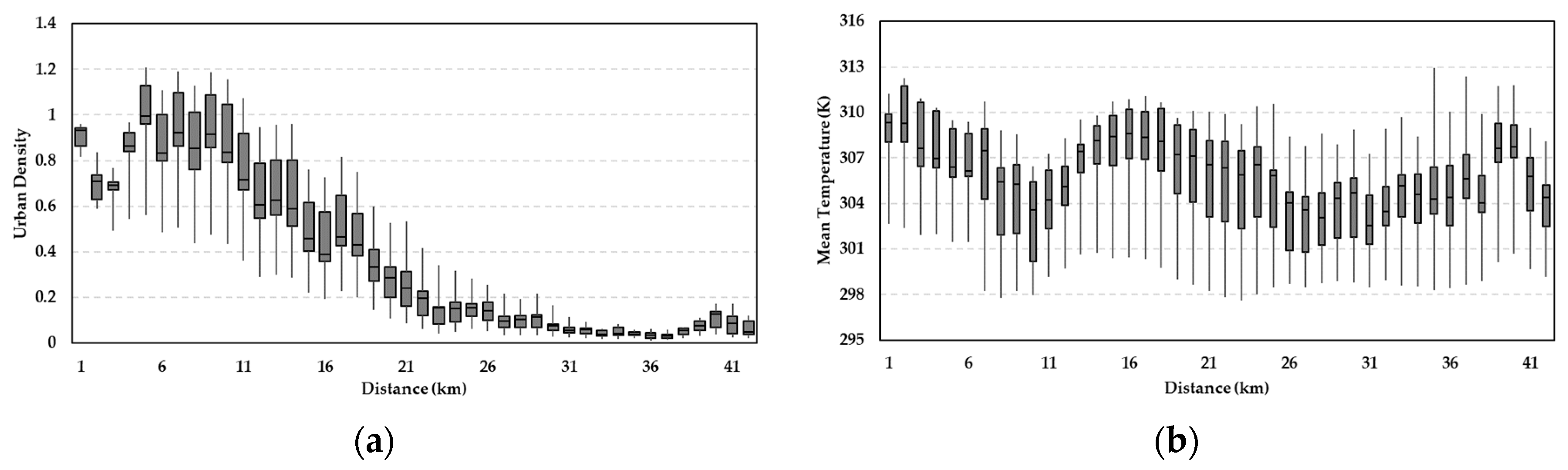
In the boxplot analysis (Figure 8), we combined both the urban density and LST values with their distance. If the median values of urban density are equal to 0.5, then there are buffer areas with both high and low urban density values. As an example, in ring 3 there are values both higher than 0.5 and lower than 0.5; overall the urban density is lower. The results can be explained better by the urban growth theory of diffusion, which was discussed earlier. When the city grows with time, a single city center will be replaced by multiple city centers. This means that selecting Colombo as a single city center is not effective when studying a time series. We therefore conducted further analysis using a gravity model.
4.3.2. Gravity Model
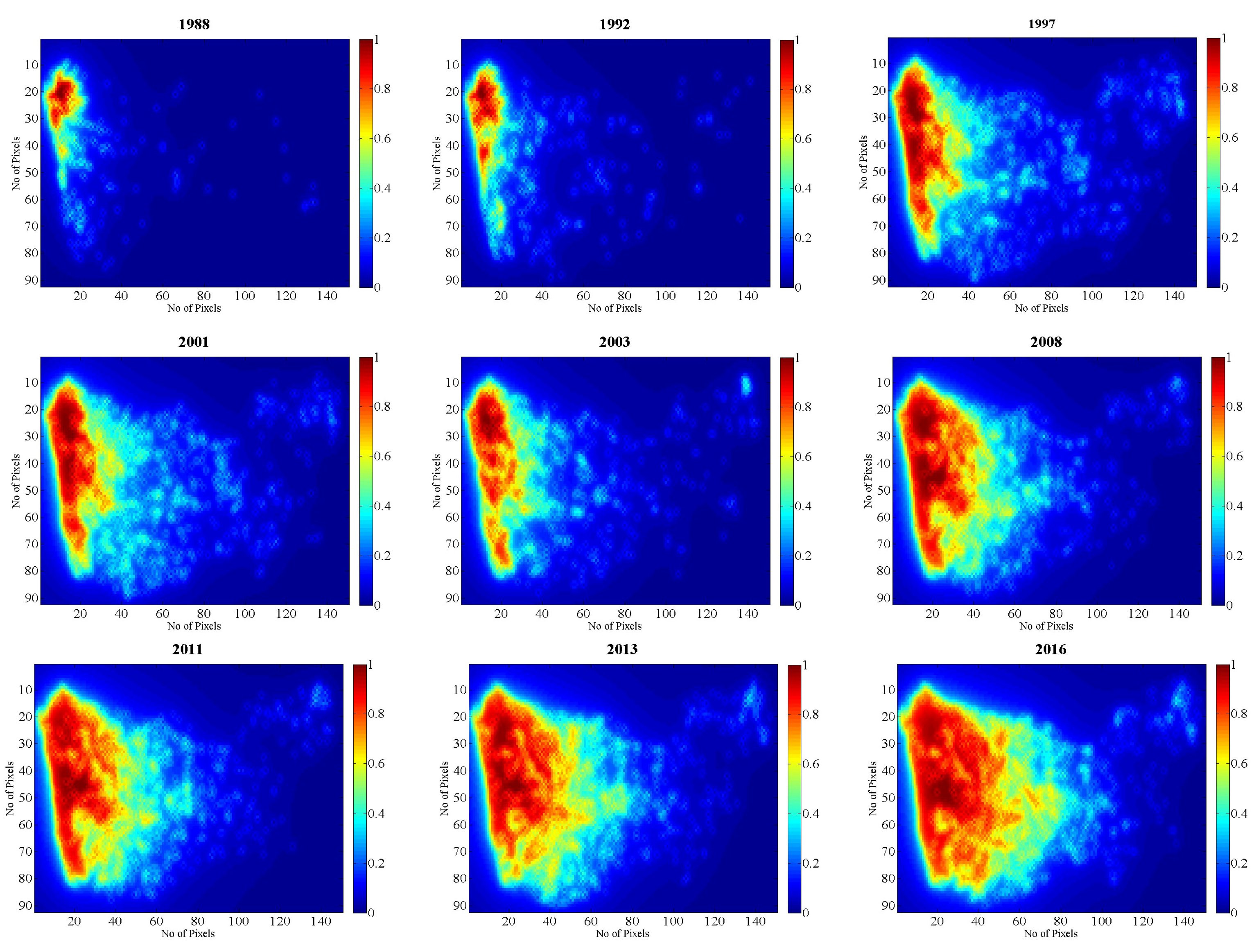
We used a gravity model to calculate the urban density based on the idea that urban density is always influenced by surrounding factors (Figure 10). Urban density for each pixel was calculated from its impact from other pixels, following the methods described in Section 3.3.2. The percentage of urbanization of a pixel depends on the amount of the pixel with urban land cover. For better visualization of the density, after calculating the gravity of each pixel as urban density, it was normalized to a scale between 0 and 1.
The main purpose of applying contouring is to make the map more readable. To summarize the figure, the dark red pixels that represent values between 0.9 and 1, and therefore represent highly urbanized areas, have moved from Colombo to different locations as time has progressed. However, Colombo remains dark, showing that, along with other cities, it is still highly urbanized. From 1988 to 2016 the high urban density area increased significantly.
As urbanization has expanded worldwide, different concepts have been developed to understand it, and the gravity model is one of the concepts used in urban geography. The gravity model is widely used in market analysis [43]. The model provides answers for most problems, like shopping center location, population and migration forecasting, traffic flow analysis, and allocation of land for residential, business, industrial, and other uses. Although in social science this concept has been used for a long time, its applications are not adequate. It is rare to find it applied to the fields of remote sensing and Geographic Information Systems (GIS). There is an emerging concept called the ‘multicity center’, and this study shows that the gravity model provides a means of understanding this.
4.3.3. Comparison of the Multi-Buffer Ring and Gravity Model
To quantitatively compare the multi-buffer ring and gravity model, correlation coefficients were calculated for the regression analyses between the average urban densities and mean LST values, both of which were derived from the multi-buffer ring and gravity model, respectively (Table 4). The correlation coefficients are positive, and become higher and higher from 1988 to 2016. In 1988, there is a moderate correlation between LST and urban density at 0.468782, but in 2016 it increased to 0.949624, showing high correlation. Having positive correlation indicates that the greater the built up area, the higher the average temperature. This implies that the relationship between the temperature and urban density is becoming stronger through time [47]. The regression analysis reveals that increasing urban density can contribute to the increase of land surface temperature in this study area.
For the gravity model, it revealed the same pattern: that LST is increasing with the growth of the city. For 1988, the correlation coefficient is 0.2254, and it is 0.5873 for 2016, as presented in Table 3. As for the multi-buffer ring method, the linear relationship is positive, but the relationship is weaker than in the multi-buffer ring method. From a lower positive correlation, it becomes a moderate correlation by 2016, which is consistent with the study described in [20]. This positive coefficient suggests that temperature increase becomes stronger as the city grows larger. There may be other reasons for the temperature rise, but our results suggest that urbanization is a significant cause. When the urban area increases, the urban population is increasing too, contributing heat discharge through human activities [50,52].
Therefore, it is reasonable to conclude that the larger the urban percentage values are, the greater the temperature values will be. Using the two above methods, it was clear that there was a significant impact on LST from urbanization. This highlights the fact that the increase in urban areas can indeed have a strong influence on local climate; but on the other hand, by mitigating the urban temperature values, it can decrease surface warming.
5. Discussion
5.1. Comparison between Colombo and Other South Asia Cities
Urban growth is common in many South Asia countries, while their growing process and patterns are different due to different urban planning and administration policies as well as their different urban landscape. Many South Asia cities were studied using satellite images and dramatic urbanization was often reported in these studies [9,10,11,13,53]. The urbanization amplitude of most major cities, such as Mumbai, Delhi, Hanoi, and Dhaka, was reported to be similar to that in Colombo of this study according to their urban land cover changes [7,9,10]. The relationship between LST and urban land use or land cover types were investigated with similar correlation [9,12,13,54]. However, the usage of satellite images was different in different studies. Studies using satellite images at two or three different dates were the most common [7,8,9,10]. All available clear-sky images within several years were conducted in Bangkok and Mumbai [11,12]. Since South Asia is located in a tropical and subtropical region, clouds contamination is a common problem for the application of optical remote sensing for urban observations, which is also indicated in most existing studies. Therefore, multi-source satellite images, especially the incorporation of microwave radar data, were recommended for future studies in South Asia.
5.2. Impacts of the Loss of Vegetation Due to Urbanization
The vegetation in the Colombo Metropolitan Area was mainly cropland and forest. However, due to the spectral similarity of the two vegetation types, it is difficult to accurately separate them with the 30-m resolution Landsat images. Generally, as demonstrated in Figure 4, the vegetation decreased from over 600 km2 to near 400 km2, with a decrease of over 33%. There are several negative impacts of this remarkable loss of vegetation. First, since these vegetation areas include a large amount of cropland, it is destructive of the local agriculture. Second, the ecosystem is also threatened, due to the significant decrease of both forest and the agricultural ecosystem, due to which the ecological services are weakened. Third, the conversion of this large area of vegetation to an urban area could contribute significantly to the urban heat island effects of the Colombo Metropolitan Area by increasing the LST.
5.3. Limitations of the Research
This study has investigated urbanization and its impacts on land surface temperature, using socio-economic concepts and theories in geography, as well as remote sensing and GIS tools. Although several studies have been conducted by urban planners and researchers in the GIS and remote sensing fields, there is still a lack of collaboration among these communities. The results of regression analysis indicated a significant relationship that becomes stronger through time, indicating that urbanization has had a great impact on the surface warming. The results will be useful to urban planners and building designers, so that they can form proposals to mitigate the temperature rise and improve the health of the city. Although we establish a linear relationship between urbanization and LST, further studies can be conducted to investigate the nonlinear relationships, combined with in situ measurements of temperature and precipitation.
However, there are some limitations evident. One of the limitations is the effect of cloud cover, which affects the classification quality in thermal remote sensing. Landsat thermal bands cannot penetrate thin cloud, which can reduce the accuracy of the temperature results. Since the study area is located on the equator, most optical satellite images contain cloud cover, which is hard to avoid. Although there are several methods for retrieving temperature values, they still need to be improved to reduce the effect of thin cloud and other atmospheric conditions.
6. Conclusions
Several conclusions can be summarized from this research. First, urban land cover maps over the study area are consistent with many concepts in urban geography. One of these concepts is that in developing countries, people are attracted to the city for social and economic opportunities, and this can be seen by the expansion of the urban area of Colombo. Second, the urban growth theory of diffusion is demonstrated in most developing countries. When a city expands, there will be more centers than the original core center—Colombo shows the early stage of this diffusion pattern. Third, Sri Lanka is recognized as being vulnerable to climate change due to its location. Being a small country in the Indian Ocean, the coastal regions especially are becoming highly vulnerable. Colombo, which is a coastal city and urbanizing rapidly, is also becoming susceptible. When the Indian Ocean tsunami occurred in 2004, it caused numerous casualties and extensive infrastructure damage, indicating that the coastal zone is vulnerable to sea level rise in the future. Fourth, the temperature values obtained from the study show a continual increase of temperature. Being a developing country, the data network from meteorological stations is not well established compared to those in developed countries. Thermal remote sensing provides a better option for this, instead of using meteorological data from in situ measurements. Last but not least, the multiple-buffer ring method was used to illustrate and create the spatial domain. The multiple-buffer ring method is known as a simple spatial analysis method in GIS, but our results show that it can be used effectively for studying complex relationships like those between urban density and temperature. Although the gravity model is widely used in studies of trade marketing and migration patterns, we found no studies where it had been applied to urban studies. Based on our results, both methods can be used effectively, but the choice will depend on the urban expansion pattern of the area. The results provide a scientific reference for policy makers and urban planners working towards a healthy and sustainable Colombo Metropolitan Area.
Author Contributions
H.P.U.F. and H.Z. conceived and designed the experiments; H.P.U.F. and Y.L. performed the experiments; H.P.U.F., H.Z., S.H., Y.S., and H.L. analyzed the results; H.P.U.F. wrote the paper; H.Z., S.H., and Y.S. revised the paper.
Funding
This research was funded by the Key Laboratory of Spatial Data Mining and Information Sharing of the Ministry of Education, Fuzhou University grant number 2016LSDMIS02, the National Natural Science Foundation of China grant number 41401370, and the Research Grants Council (RGC) General Research Fund grant numbers 14601515, 14635916, and 14605917.
Acknowledgments
The authors would like to thank the two anonymous reviewers for their critical comments and suggestions to improve the original manuscript.
Conflicts of Interest
The authors declare no conflict of interest.
References
- Spence, M.; Annez, P.; Buckley, R. Urbanization and Growth; World Bank: Washington, DC, USA, 2009. [Google Scholar]
- UN-Habitat. Un Habitat for a Better Urban Future. Available online: https://unhabitat.Org/urban-themes/climate-change/ (accessed on 20 April 2019).
- Oke, T.R. Boundary Layer Climates; Taylor & Francis Group: London, UK, 1987. [Google Scholar]
- Benenson, W.; Harris, J.W.; Stöcker, H.; Lutz, H. Handbook of Physics; Springer: New York, NY, USA, 2002. [Google Scholar]
- Carleton, T.A.; Hsiang, S.M. Social and economic impacts of climate. Science 2016, 353. [Google Scholar] [CrossRef]
- Fu, P.; Weng, Q.H. A time series analysis of urbanization induced land. Use and land cover change and its impact on land surface temperature with landsat imagery. Remote Sens. Environ. 2016, 175, 205–214. [Google Scholar] [CrossRef]
- Hoan, N.T.; Liou, Y.A.; Nguyen, K.A.; Sharma, R.C.; Tran, D.P.; Liou, C.L.; Cham, D.D. Assessing the effects of land-use types in surface urban heat islands for developing comfortable living in hanoi city. Remote Sens. 2018, 10, 1965. [Google Scholar] [CrossRef]
- Sharma, R.; Joshi, P.K. Monitoring urban landscape dynamics over Delhi (India) using remote sensing (1998–2011) inputs. J. Indian Soc. Remote Sens. 2013, 41, 641–650. [Google Scholar] [CrossRef]
- Ahmed, B.; Kamruzzaman, M.; Zhu, X.; Rahman, M.S.; Choi, K. Simulating land cover changes and their impacts on land surface temperature in Dhaka, Bangladesh. Remote Sens. 2013, 5, 5969–5998. [Google Scholar] [CrossRef]
- Rahman, A.; Kumar, S.; Fazal, S.; Siddiqui, M.A. Assessment of land use/land cover change in the north-west district of delhi using remote sensing and gis techniques. J. Indian Soc. Remote Sens. 2012, 40, 689–697. [Google Scholar] [CrossRef]
- Zhang, H.S.; Wang, T.; Zhang, Y.H.; Dai, Y.R.; Jia, J.J.; Yu, C.; Li, G.; Lin, Y.Y.; Lin, H.; Cao, Y. Quantifying short-term urban land cover change with time series landsat data: A comparison of four different cities. Sensors 2018, 18, 4319. [Google Scholar] [CrossRef]
- Keeratikasikorn, C.; Bonafoni, S. Urban heat island analysis over the land use zoning plan of bangkok by means of landsat 8 imagery. Remote Sens. 2018, 10, 440. [Google Scholar] [CrossRef]
- Sultana, S.; Satyanarayana, A.N.V. Urban heat island intensity during winter over metropolitan cities of india using remote-sensing techniques: Impact of urbanization. Int. J. Remote Sens. 2018, 39, 6692–6730. [Google Scholar] [CrossRef]
- Killian, J. Magnet-Cities. Available online: https://home.Kpmg.Com/uk/en/home/insights/2014/07/magnet-cities.Html (accessed on 14 July 2014).
- Rahman, M.T. Detection of land use/land cover changes and urban sprawl in al-khobar, Saudi Arabia: An analysis of multi-temporal remote sensing data. Int. J. Geo Inf. 2016, 5, 15. [Google Scholar] [CrossRef]
- Sun, H.; Forsythe, W.; Waters, N. Modeling urban land use change and urban sprawl: Calgary, Alberta, Canada. Netw. Spat. Econ. 2007, 7, 353–376. [Google Scholar] [CrossRef]
- Survey Department. Area of Sri Lanka by Province and District; Department of Census and Statistics: Battaramulla, Sri Lanka, 2011.
- Young, N.E.; Anderson, R.S.; Chignell, S.M.; Vorster, A.G.; Lawrence, R.; Evangelista, P.H. A survival guide to landsat preprocessing. Ecology 2017, 98, 920–932. [Google Scholar] [CrossRef]
- Amiri, R.; Weng, Q.H.; Alimohammadi, A.; Alavipanah, S.K. Spatial-temporal dynamics of land surface temperature in relation to fractional vegetation cover and land use/cover in the Tabriz urban area, Iran. Remote Sens. Environ. 2009, 113, 2606–2617. [Google Scholar] [CrossRef]
- Ibrahim, G.R.F. Urban land use land cover changes and their effect on land surface temperature: Case study using dohuk city in the Kurdistan region of Iraq. Climate 2017, 5, 13. [Google Scholar] [CrossRef]
- Meng, F.; Liu, M. Remote-sensing image-based analysis of the patterns of urban heat islands in rapidly urbanizing Jinan, China. Int. J. Remote Sens. 2013, 34, 8838–8853. [Google Scholar] [CrossRef]
- Congalton, R.G.; Green, K. Assessing the Accuracy of Remotely Sensed Data: Principles and Practices; CRC Press/Taylor & Francis: Boca Raton, FL, USA, 2009. [Google Scholar]
- Pal, M. Ensemble of support vector machines for land cover classification. Int. J. Remote Sens. 2008, 29, 3043–3049. [Google Scholar] [CrossRef] [Green Version]
- Pal, M.; Mather, P.M. Support vector machines for classification in remote sensing. Int. J. Remote Sens. 2005, 26, 1007–1011. [Google Scholar] [CrossRef]
- Xu, R.; Zhang, H.S.; Lin, H. Urban impervious surfaces estimation from optical and SAR imagery: A comprehensive comparison. IEEE J. Sel. Top. Appl. Earth Obs. Remote Sens. 2017, 10, 4010–4021. [Google Scholar] [CrossRef]
- Zhang, H.; Li, J.; Wang, T.; Lin, H.; Zheng, Z.; Li, Y.; Lu, Y. A manifold learning approach to urban land cover classification with optical and radar data. Landsc. Urban Plan. 2018, 172, 11–24. [Google Scholar] [CrossRef]
- Zhang, H.; Lin, H.; Wang, Y. A new scheme for urban impervious surface classification from SAR images. ISPRS J. Photogramm. Remote Sens. 2018, 139, 103–118. [Google Scholar] [CrossRef]
- Zhang, H.S.; Zhang, Y.Z.; Lin, H. A comparison study of impervious surfaces estimation using optical and SAR remote sensing images. Int. J. Appl. Earth Obs. 2012, 18, 148–156. [Google Scholar] [CrossRef]
- Zhang, Y.Z.; Zhang, H.S.; Lin, H. Improving the impervious surface estimation with combined use of optical and SAR remote sensing images. Remote Sens. Environ. 2014, 141, 155–167. [Google Scholar] [CrossRef]
- Breiman, L. Random forests. Mach. Learn. 2001, 45, 5–32. [Google Scholar] [CrossRef]
- Stumpf, A.; Kerle, N. Object-oriented mapping of landslides using random forests. Remote Sens. Environ. 2011, 115, 2564–2577. [Google Scholar] [CrossRef]
- Gislason, P.O.; Benediktsson, J.A.; Sveinsson, J.R. Random forests for land cover classification. Pattern Recogn. Lett. 2006, 27, 294–300. [Google Scholar] [CrossRef]
- Qin, Z.; Karnieli, A.; Berliner, P. A mono-window algorithm for retrieving land surface temperature from landsat tm data and its application to the Israel-Egypt border region. Int. J. Remote Sens. 2001, 22, 3719–3746. [Google Scholar] [CrossRef]
- Sobrino, J.A.; Jimenez-Munoz, J.C.; Paolini, L. Land surface temperature retrieval from landsat tm 5. Remote Sens. Environ. 2004, 90, 434–440. [Google Scholar] [CrossRef]
- Jimenez-Munoz, J.C.; Sobrino, J.A. A generalized single-channel method for retrieving land surface temperature from remote sensing data. JGR Atmos. 2003, 108. [Google Scholar] [CrossRef] [Green Version]
- Stathopoulou, M.; Cartalis, C. Daytime urban heat islands from landsat etm+ and corine land cover data: An application to major cities in Greece. Sol. Energy 2007, 81, 358–368. [Google Scholar] [CrossRef]
- Weng, Q.H. Thermal infrared remote sensing for urban climate and environmental studies: Methods, applications, and trends. ISPRS J. Photogramm. Remote Sens. 2009, 64, 335–344. [Google Scholar] [CrossRef]
- Weng, Q.H.; Lu, D.S.; Schubring, J. Estimation of land surface temperature-vegetation abundance relationship for urban heat island studies. Remote Sens. Environ. 2004, 89, 467–483. [Google Scholar] [CrossRef]
- Chander, G.; Markham, B.L.; Helder, D.L. Summary of current radiometric calibration coefficients for landsat mss, tm, etm+, and eo-1 ali sensors. Remote Sens. Environ. 2009, 113, 893–903. [Google Scholar] [CrossRef]
- Mishra, N.; Haque, M.O.; Leigh, L.; Aaron, D.; Helder, D.; Markham, B. Radiometric cross calibration of landsat 8 operational land imager (oli) and landsat 7 enhanced thematic mapper plus (etm plus). Remote Sens. 2014, 6, 12619–12638. [Google Scholar] [CrossRef]
- Sobrino, J.A.; Raissouni, N. Toward remote sensing methods for land cover dynamic monitoring: Application to morocco. Int. J. Remote Sens. 2000, 21, 353–366. [Google Scholar] [CrossRef]
- Tobler, W.R. A computer movie simulating urban growth in the Detroit region. Econ. Geogr. 1970, 46, 234. [Google Scholar] [CrossRef]
- Carrothers, G.A. An historical bedew of the gravity and potential concepts of human interaction. J. Am. Inst. Plan. 1956, 22, 94–102. [Google Scholar] [CrossRef]
- Zhang, H.S.; Xu, R. Exploring the optimal integration levels between sar and optical data for better urban land cover mapping in the pearl river delta. Int. J. Appl. Earth Obs. 2018, 64, 87–95. [Google Scholar] [CrossRef]
- Subasinghe, S.; Estoque, R.C.; Murayama, Y. Spatiotemporal analysis of urban growth using GIS and remote sensing: A case study of the Colombo metropolitan area, Sri Lanka. ISPRS Int. J. Geo Inf. 2016, 5, 197. [Google Scholar] [CrossRef]
- Estoque, R.C.; Murayama, Y. Intensity and spatial pattern of urban land changes in the megacities of Southeast Asia. Land Use Policy 2015, 48, 213–222. [Google Scholar] [CrossRef]
- Tran, D.X.; Pla, F.; Latorre-Carmona, P.; Myint, S.W.; Gaetano, M.; Kieu, H.V. Characterizing the relationship between land use land cover change and land surface temperature. ISPRS J. Photogramm. Remote Sens. 2017, 124, 119–132. [Google Scholar] [CrossRef] [Green Version]
- Ding, H.Y.; Shi, W.Z. Land-use/land-cover change and its influence on surface temperature: A case study in Beijing city. Int. J. Remote Sens. 2013, 34, 5503–5517. [Google Scholar] [CrossRef]
- Gong, A.D.; Chen, Y.H.; Li, J.; Gong, H.L.; Li, X.J. Spatial distribution patterns of the urban heat island based on remote sensing images: A case study in Beijing, China. In Proceedings of the 2006 IEEE International Geoscience Remote Sensing Symposium, Denver, CO, USA, 31 July–4 August 2006. [Google Scholar] [CrossRef]
- Youneszadeh, S.; Amiri, N.; Pilesjo, P. The effect of land use change on land surface temperature in the Netherlands. In Proceedings of the International Conference on Sensors & Models in Remote Sensing & Photogrammetry, Kish Island, Iran, 23–25 November 2015; Volume 41, pp. 745–748. [Google Scholar]
- Dietzel, C.; Oguz, H.; Hemphill, J.J.; Clarke, K.C.; Gazulis, N. Diffusion and coalescence of the Houston metropolitan area: Evidence supporting a new urban theory. Environ. Plan. B 2005, 32, 231–246. [Google Scholar] [CrossRef]
- Zhou, W.Q.; Qian, Y.G.; Li, X.M.; Li, W.F.; Han, L.J. Relationships between land cover and the surface urban heat island: Seasonal variability and effects of spatial and thematic resolution of land cover data on predicting land surface temperatures. Landsc. Ecol. 2014, 29, 153–167. [Google Scholar] [CrossRef]
- Kamini, J.; Jayanthi, S.C.; Raghavswamy, V. Spatio-temporal analysis of land use in urban mumbai-using multi-sensor satellite data and GIS techniques. J. Indian Soc. Remote Sens. 2006, 34, 385–396. [Google Scholar] [CrossRef]
- Estoque, R.C.; Murayama, Y.; Myint, S.W. Effects of landscape composition and pattern on land surface temperature: An urban heat island study in the megacities of Southeast Asia. Sci. Total Environ. 2017, 577, 349–359. [Google Scholar] [CrossRef] [PubMed]
Figure 1.
Maps of (a) Sri Lanka and (b) Colombo Metropolitan Area.

Figure 2.
Sampling strategies for collecting the reference samples from high resolution Google Earth images.
Figure 2.
Sampling strategies for collecting the reference samples from high resolution Google Earth images.

Figure 3.
The results of classification using support vector machine (SVM) in Colombo between 1988 and 2016.
Figure 3.
The results of classification using support vector machine (SVM) in Colombo between 1988 and 2016.
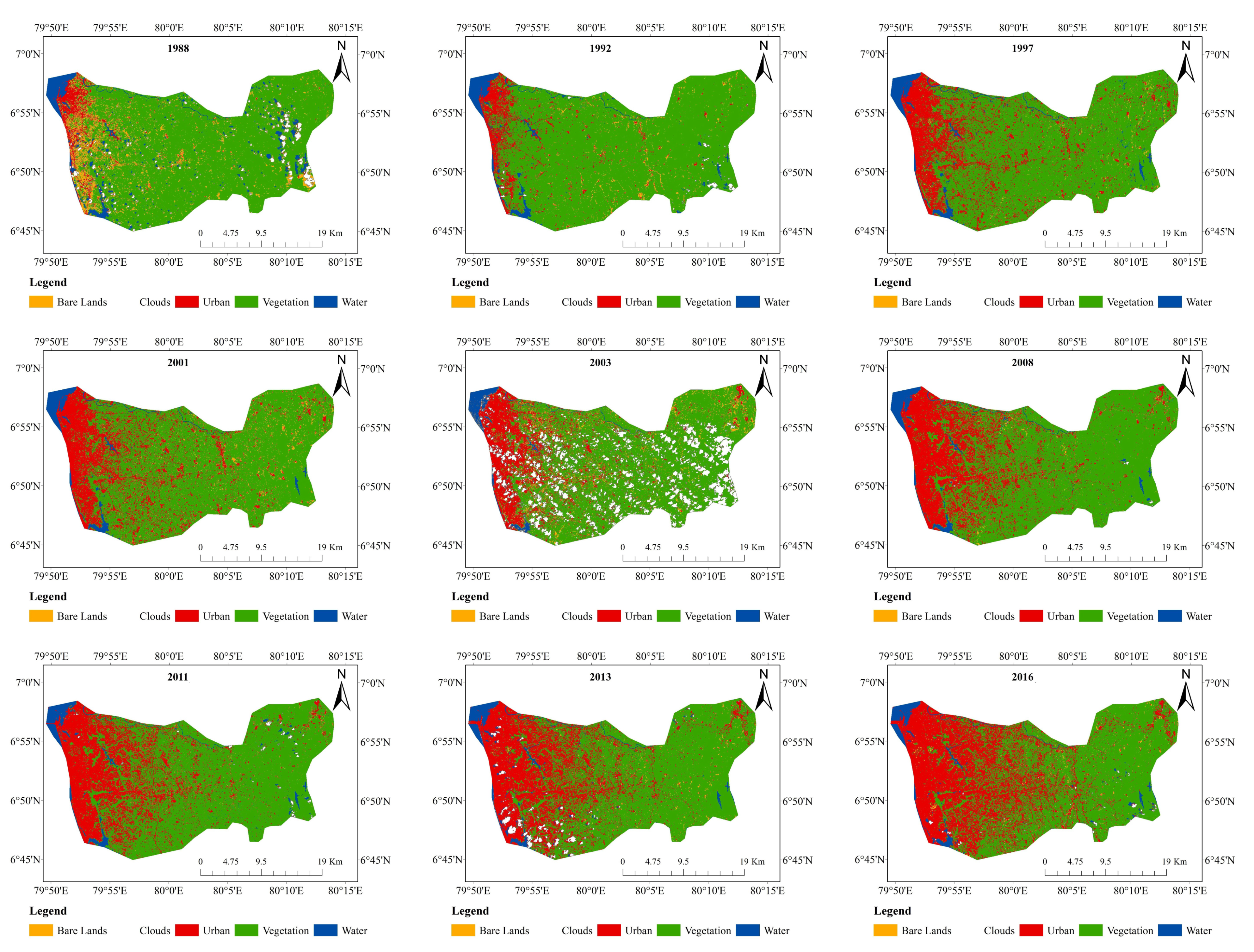
Figure 4.
The results of classification using random forest (RF) in Colombo between 1988 and 2016.
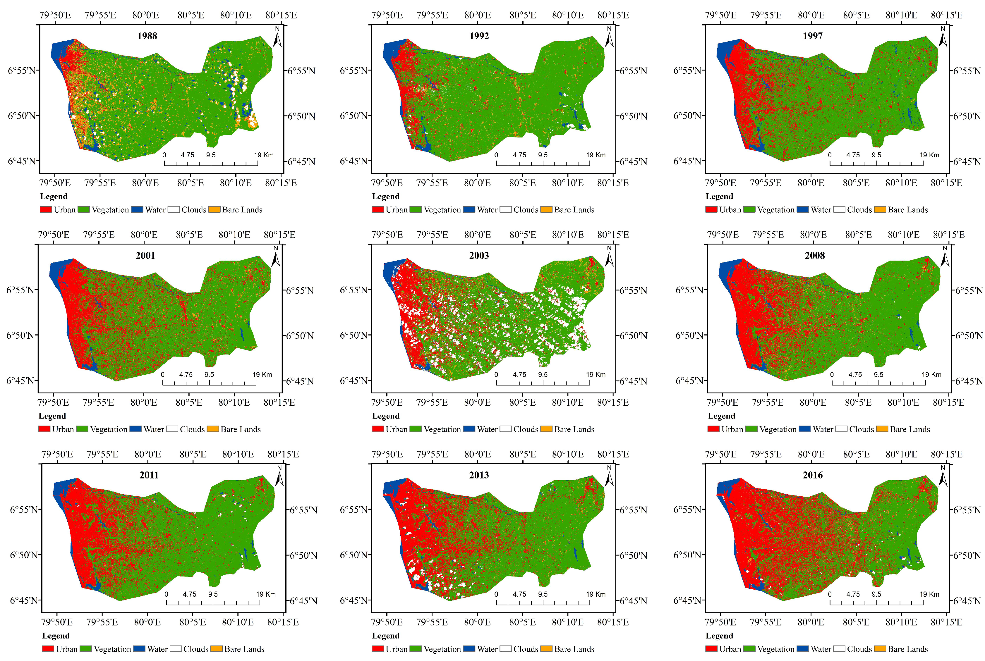
Figure 5.
Urban land cover change in Colombo from 1988 to 2016.

Figure 6.
Annual Land Surface Temperature for corresponding years to land cover classification.

Figure 7.
Multi-buffer ring analysis of Colombo from 1988 to 2016.

Figure 8.
Trend analysis of (a) average urban density and (b) average temperature with distance from the city center.
Figure 8.
Trend analysis of (a) average urban density and (b) average temperature with distance from the city center.
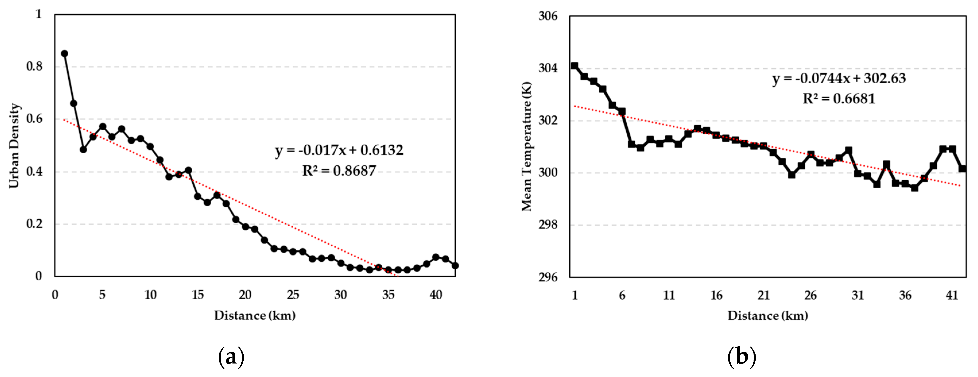
Figure 9.
Boxplot analysis of (a) urban density range from the city center and (b) temperature variations from the city center.
Figure 9.
Boxplot analysis of (a) urban density range from the city center and (b) temperature variations from the city center.

Figure 10.
Gravity model of urban density from 1988 to 2016.

Table 1.
Information about Landsat images used in this study.
| ID | Sensor Type | Acquisition Date | Path/Row | Spatial Resolution |
|---|---|---|---|---|
| LT51410551988350BKT01 | TM | 1988-12-15 | 141/55 | 30 m |
| LT51410551992073BKT01 | TM | 1992-03-13 | 141/55 | 30 m |
| LT51410551994094BKT01 | TM | 1994-04-04 | 141/55 | 30 m |
| LT51410551997038BKT01 | TM | 1997-02-07 | 141/55 | 30 m |
| LE71410552001041SGS00 | ETM | 2001-02-10 | 141/55 | 30 m |
| LT51410552003343BKT00 | TM | 2003-12-09 | 141/55 | 30 m |
| LT51410552008309BKT00 | TM | 2008-11-04 | 141/55 | 30 m |
| LT51410552011317BKT00 | TM | 2011-11-13 | 141/55 | 30 m |
| LC81410552013242LGN00 | OLI_TIRS | 2013-08-30 | 141/55 | 30 m |
| LC81410552016027LGN00 | OLI_TIRS | 2016-01-27 | 141/55 | 30 m |
Table 2.
Overall accuracy and Kappa coefficient of the classification.
| SVM | RF | |||
|---|---|---|---|---|
| Year | Overall Accuracy | Kappa Coefficient | Overall Accuracy | Kappa Coefficient |
| 1988 | 87.04% | 0.7751 | 86.12% | 0.7643 |
| 1992 | 93.96% | 0.901 | 93.81% | 0.898 |
| 1997 | 85.13% | 0.7306 | 85.47% | 0.7259 |
| 2001 | 82.91% | 0.7515 | 80.30% | 0.7159 |
| 2003 | 93.79% | 0.9036 | 93.28% | 0.8958 |
| 2007 | 94.51% | 0.9157 | 93.72% | 0.9036 |
| 2011 | 96.32% | 0.9432 | 96.21% | 0.9415 |
| 2013 | 84.74% | 0.7961 | 92.28% | 0.8581 |
| 2016 | 97.25% | 0.9467 | 97.21% | 0.9455 |
Table 3.
Mean Land Surface Temperature for corresponding urban land covers (in Kelvin).
| 1988 | 1992 | 1997 | 2001 | 2003 | 2008 | 2011 | 2013 | 2016 | |
|---|---|---|---|---|---|---|---|---|---|
| Water | 292.1813 | 292.9454 | 293.154 | 294.3133 | 296.1483 | 296.468 | 296.4978 | 296.766 | 297.4211 |
| Vegetation | 295.3342 | 295.9467 | 297.8987 | 298.4418 | 300.4154 | 300.6984 | 300.9962 | 301.107 | 301.2562 |
| Bare Land | 295.6886 | 296.8361 | 299.268 | 299.4706 | 301.1288 | 301.3109 | 302.2325 | 302.5835 | 304.3118 |
| Urban | 295.3342 | 298.3201 | 300.2554 | 300.8821 | 302.1098 | 302.4714 | 303.4135 | 304.2593 | 304.27 |
Table 4.
Correlation coefficients between average urban densities and mean LST derived from the multi-buffer ring method and gravity model.
Table 4.
Correlation coefficients between average urban densities and mean LST derived from the multi-buffer ring method and gravity model.
| Year | 1988 | 1992 | 1994 | 1997 | 2001 | 2003 | 2008 | 2011 | 2013 | 2016 |
|---|---|---|---|---|---|---|---|---|---|---|
| Multi-buffer Ring | 0.4688 | 0.5307 | 0.7414 | 0.7960 | 0.7961 | 0.8156 | 0.8796 | 0.9258 | 0.9463 | 0.9496 |
| Gravity Model | 0.2254 | 0.2941 | 0.3654 | 0.4089 | 0.4698 | 0.4790 | 0.4800 | 0.4931 | 0.5330 | 0.5873 |
© 2019 by the authors. Licensee MDPI, Basel, Switzerland. This article is an open access article distributed under the terms and conditions of the Creative Commons Attribution (CC BY) license (http://creativecommons.org/licenses/by/4.0/).
Share and Cite
MDPI and ACS Style
Fonseka, H.P.U.; Zhang, H.; Sun, Y.; Su, H.; Lin, H.; Lin, Y. Urbanization and Its Impacts on Land Surface Temperature in Colombo Metropolitan Area, Sri Lanka, from 1988 to 2016. Remote Sens. 2019, 11, 957. https://doi.org/10.3390/rs11080957
AMA Style
Fonseka HPU, Zhang H, Sun Y, Su H, Lin H, Lin Y. Urbanization and Its Impacts on Land Surface Temperature in Colombo Metropolitan Area, Sri Lanka, from 1988 to 2016. Remote Sensing. 2019; 11(8):957. https://doi.org/10.3390/rs11080957
Chicago/Turabian StyleFonseka, H.P.U., Hongsheng Zhang, Ying Sun, Hua Su, Hui Lin, and Yinyi Lin. 2019. "Urbanization and Its Impacts on Land Surface Temperature in Colombo Metropolitan Area, Sri Lanka, from 1988 to 2016" Remote Sensing 11, no. 8: 957. https://doi.org/10.3390/rs11080957
Note that from the first issue of 2016, this journal uses article numbers instead of page numbers. See further details here.