Towards Automatic Extraction and Updating of VGI-Based Road Networks Using Deep Learning


1
Department of Electrical Engineering and Computer Science, Khalifa University, Masdar City, P.O. Box 54224, Abu Dhabi, UAE
2
Department of Information Engineering and Computer Science, University of Trento, via Sommarive, 9, 38123 Trento, Italy
*
Author to whom correspondence should be addressed.
Remote Sens. 2019, 11(9), 1012; https://doi.org/10.3390/rs11091012
Submission received: 18 March 2019
/
Revised: 15 April 2019
/
Accepted: 24 April 2019
/
Published: 28 April 2019
(This article belongs to the Section Remote Sensing Image Processing)
Abstract
:This work presents an approach to road network extraction in remote sensing images. In our earlier work, we worked on the extraction of the road network using a multi-agent approach guided by Volunteered Geographic Information (VGI). The limitation of this VGI-only approach is its inability to update the new road developments as it only follows the VGI. In this work, we employ a deep learning approach to update the road network to include new road developments not captured by the existing VGI. The output of the first stage is used to train a Convolutional Neural Network (CNN) in the second stage to generate a general model to classify road pixels. Post-processing is used to correct the undesired artifacts such as buildings, vegetation, occlusions, etc. to generate a final road map. Our proposed method is tested on the satellite images acquired over Abu Dhabi, United Arab Emirates and the aerial images acquired over Massachusetts, United States of America, and is observed to produce accurate results.
1. Introduction
In our earlier work, we worked on extraction of roads guided by Volunteered Geographic Information (VGI) [1]. VGI is collected using crowd-sourcing tools which allow general public to contribute towards a global database that contains geo-referenced data about the Earth’s surface. OpenStreetMap (OSM) is one such example, which provides spatial, geometrical, and attribute information about road networks, building footprints, landmarks, etc. In the case of roads, VGI data is often provided only as vector data represented by lines and not as full extent. Also, depending the geo-registration accuracy of the base maps, the VGI data can consist of significant errors. Our previous approach works based on the assumption that road segments are always connected with local geometrical homogeneity. By using the direction of the segments in VGI, we extract the full extent of the roads in the remotely sensed images. However, the limitation of this VGI-only approach is its inability to update the new road developments which are not captured in VGI; In this paper, we introduce an approach based on Convolutional Neural Network (CNN) to extract the complete network by also extracting segments that are not available in the VGI. The output of the first stage where VGI is used to extract the full extent of the road is employed as a labelled class input to train the CNN in the second stage. Furthermore, post-processing is performed to correct undesired non-road artifacts such as buildings, vegetation, occlusions, etc. In the third stage, we develop a graph-theoretic approach as a post-processing step to enhance the accuracy of the extracted road network by connecting disjoint road segments.
In the last few years, the deep CNN architectures have quickly become prominent in many remote sensing applications since they have the ability to effectively use spectral and spatial information without needing any prepossessing step. A CNN is composed of multiple interconnected layers and learns a hierarchical feature representation from lower-level pixel data as it discovers features in multiple levels of representations. The lowest level is depicted by the primitive features of pixels (e.g., spectral properties). The higher level involves transforming from the raw pixel representation into gradually more abstract representations that are invariant to small geometric variations such as edges and corners. Furthermore, they are gradually transformed and made resilient to contrast changes as well as contrast inversion (i.e., object parts). The most frequent patterns related to the higher-level abstract categories that represent whole objects are identified at the end [2,3].
Deep Learning has been widely applied to various computer vision tasks [4,5] with significant success because of its superiority in terms of feature representation. In remote sensing, deep learning methods have been able to provide remarkable success in the applications such as land cover/use classification [6,7,8,9], synthetic-aperture radar (SAR) image classification [10,11], hyper-spectral image classification [3,12] as well as object recognition in remote sensing images [13,14].
The first stage of our work was reported in [1]. It makes use of a segmentation approach where autonomous agents traverse through segments in a known road direction provided by VGI to extract the full extent of the road segments. The process starts with segmentation of the input image into smaller image segments. Then, multiple parallel processes (the agents) traverse through these segments guided by the VGI to group those with similar spectral characteristics as road segments. A post-processing step which considers the general characteristics of the road objects prunes the shapes of these segments to generate homogeneous road geometry throughout the network. This approach is shown to extract full extent of the roads as shown in the example in Figure 1.
However, as can be seen in Figure 1d, the approach doesn’t extract segments (as indicated in white color in Figure 1d) which are not represented in the VGI which is often not updated regularly. The main contribution of this paper lies in introducing the following two additional stages to address the issue of automatic road network extraction and updating.
- In the second stage, we make use of the outputs from the first stage where VGI data has been used to extract an initial road network to train the CNN architecture. To our best knowledge, ours is the first attempt to use a CNN architecture with reduced context size of ‘8 × 8’ pixels for road classification based on the combination of both probabilistic pixel and patch based prediction for the purpose of road network extraction. This reduces the computational load significantly. Furthermore, we carry out post-processing to rectify the extracted road network to improve the accuracy.
- In the third stage, we connect the isolated road segments to ensure a continuous network with simple features pertaining to road’s spectral, geometric and topological information. The edges of the isolated segments are connected to the closest node in the existing network extracted in the previous steps.
2. Background and Related Works
Convolutional neural network (CNN) is a multi-level feed-forward artificial neural network belonging to the category of deep learning. A typical CNN consists of multiple layers which repeat in turn with convolutional and pooling layers, and one or more fully connected (FC) layers. The convolutional layer produces the feature maps of the previous layers with filters. The pooling layer receives smaller size rectangular blocks from the convolutional layer and further sub-samples it to obtain a single output from each block. Max pooling and average pooling are its two types. In the former, the maximum value observed in the window is sent to the next layer whereas in the latter, an average of the observed value is sent. The fully connected layer has connections to all neurons of previous layers, with each connection having its own individual weight [15].
Usually, CNN classification is performed in either patch-based mode or pixel-to-pixel-based (end-to-end) mode. In the patch-based mode, we commonly start with small image patches to train the CNN model. By using a sliding window over all the pixels to extract patches corresponding to neighborhoods around the pixels, the classes of the pixels are predicted. Also, the fully connected layers can be converted to convolutional layers, without overlapping at pixel level [16,17] to usually detect large urban objects. Pixel-based methods use an end to end CNN, where usually encoder-decoder architectures are used by applying methods like up-sampling, interpolation, etc. [18,19]. The latter approach is essential to trace fine details of the input images.
CNN is able to deliver significant performance improvement as it is shown to learn the optimal filters performing convolution operations in the image domain [20]. GoogLeNet, AlexNet, VGG-16, VGG-19 and ResNet are some of the widely used CNN frameworks in different remote sensing tasks which address problems based on performing transfer learning or with convolutional feature extraction [20]. CNNs have been widely used in literature for various applications such as speech recognition [21], natural language processing (NLP) [22], information retrieval [23], compute vision [24], and image analysis [2]. In the work of Jiang et al. [18], graph-based segmentation is integrated with CNNs to localize image patches, which help in localizing objects effectively. Lngkvist et al. [19] used CNNs along with spectral features of Simple Linear Iterative Clustering (SLIC) segmentation to improve the performance of CNNs. Zhang et al. [25] makes use of a semantic segmentation neural network approach which combines the strengths of residual learning and U-Net.
For road extraction, various classification-based, knowledge-based, mathematical morphology and dynamic programming approaches have been explored [26]. Previous works using CNN on road extraction mostly tend to detect road pixels or patches, and then uses complex post-processing heuristics to infer graph connectivity. Li et al. [27] uses CNN to get the probable road segments and then uses line integral convolution based connection scheme to connect the segments. Recently, Bastani et al. [28] used an iterative search process guided by a CNN-based decision function to derive the road network graph directly from the output of the CNN. [29] employs post-processing to make the extracted road region more realistic, several morphological algorithms are typically deployed to fill the holes, smooth the edges, connect the road segment, and then achieve the coarse center lines of road segments.
Few works use CNN also focused on composite extraction of roads and buildings together [30,31]. Saito et al. [30] used a single CNN architecture for extracting roads and buildings on the Mnih imagery dataset [32] using multi-class probability output of roads, buildings and background simultaneously. They also apply Channel-wise Inhibited Softmax (CIS) function to suppress the effect of the background. Alshehhi et al. [31] used a single patch-based CNN architecture for extraction of roads along with buildings from high-resolution remote sensing images. It uses a deeper patch-based segmentation, and a CNN consisting of a simple global average pooling layer. It also make use of a post-processing method based on low-level features such as asymmetry and compactness of adjacent regions, incorporating spatial structures to distinguish between roads and buildings. Recently, Shi et al. [33] used Generative Adversarial Networks to generate road networks which consists of generative model that produces segmentation maps by stimulating the data probability distribution of the road, and a discriminative model that helps to distinguish whether the samples are coming from generative model or the ground truth. Both generative and discriminative models form an adversarial training network to obtain final results.
3. Proposed Methodology
Figure 2 represents the block diagram using deep learning framework. In this section, we describe the three stages starting from (i) training data generation, (ii) defining CNN architecture and performing post-processing on the generated outputs, and finally (iii) completion of the road network.
3.1. Stage 1: Training Data Generation from Initial Road Extraction Using VGI
In the first stage, we use the VGI to generate an initial map of the road network as described in [1]. We use the initial network as training data for the CNN. In order to generate the training data, we extract patches of size ‘8 × 8’ pixels from input satellite images and the binary road map. The multi-spectral patches are fed as input features into CNN while the patches from output of first stage are treated as their class labels. We increase the size of the training data by rotating these patches by 90 degrees. All the training data is normalized. If at least one fourth of the pixels in the patch are classified as road pixel, then we consider the patch to be labeled as road. Finally, in order to prevent that CNN becomes biased towards one particular class, we balance the training dataset to include the same number of patches from both the classes (i.e., road and non-road classes). Patches consisting of less than one fourth of the pixels classified as road pixels are ignored in the training set as they represent ambiguous patches.
3.2. Stage 2: CNN Approach to Extract Probable Road Segments
We train a CNN to develop a general model for extracting roads and also carry out post-processing to remove non-road artifacts in the extracted road network.
3.2.1. CNN Architecture
In this work, we use a CNN model consisting of five convolutional and two fully connected layers (as shown in Figure 3) whose structure is expressed as: CL(5 × 5, 3, 8) - CL(3 × 3, 8, 8) - CL(3 × 3, 8, 16) - CL(3 × 3, 16, 32) - CL(3 × 3, 32, 64) - FC(1024, 64) - ReLU - FC(64, 2).
- CL(N × N, I, F): It represents a convolutional layer with filter size of N × N, I represents no. of image input channels, and F defines the no. of output channels obtained by using different number of filters. The default stride in both vertical and horizontal direction is 1.
- M(N × N, S): It represents max-pooling layer of size ‘N × N’ with ‘S’ unit strides.
- FC(I, O): It represents fully connected layer with ‘I’ input channels and ‘O’ output channels.
- LRNL: It represents local response normalization layer which sufficiently prevents overfitting without needing to perform additional dropout and L2 regularization.
Here, each convolutional layer is followed with rectified linear unit (ReLU) activation layer, LRNL and with a M(2 × 2, 2) max-pooling layer. The activation function used in the first FC layers is identity function while second FC has the sigmoid function. Then, softmax function is applied to two outputs to get the probabilities for two classes. Cross entropy is used as the loss function to train the weights of the network.
3.2.2. Post-Processing
In this step, the output obtained from CNN is refined by filtering out VGI detected road segments and non-road segments which includes removing buildings and other occlusions, etc. In classification of remote sensing images, occlusions such as buildings, parking lots, etc. often tend to be identified as roads, as they are made out of similar materials and share similar spectral characteristics. The segments extracted in the first step based on VGI are used directly and only the updated segments are processed.
The post-processing consists of the following components:
- Identifying building regions: In our proposed method, in order to remove buildings, we utilize an approach which uses image segmentation for detecting building regions [34]. The method uses image segmentation to segment the images into smaller segments and detect buildings as segments with high contrast to the darkest segment in the neighborhood in the direction of the expected shadows based on the sun angle.
- Vegetation and Shadows: To avoid confusion between vegetation and shadow regions, normalized difference vegetation index (NDVI) values are used. Shadows are expected to have NDVI values lower than 0 and vegetation is expected to have values greater than 0.3. The thresholds are chosen based on manual observation across the test images.
- Removing Parking Lots: To remove the remaining non-road artifacts like parking lots, we analyze the number of branches in skeletons of the segments additionally added to the initial road network extracted using VGI. The skeleton of non-road segments such as parking lots tend to have more number of branch points as compared to road segments which are much smoother.It can be seen that road segments are often smooth and continuous segments which consists of fewer branches in the skeleton. However, areas like parking lots are wider and asymmetric. So, the skeletons of such objects have higher number of branches. We use the ratio of Area to Branch points as the indicator to discriminate between road/non-road segments. We set the threshold to 0.0025 based on the observation of various road segments in the test images.
3.3. Stage 3: Completion of Road Network
The final stage consists of the process to ensure that all road segments are connected in a network. It makes use of end points of detected road segments as nodes, and defines a way to connect disjoint segments to form a complete road network.The building blocks of our road network are the road segments after post-processing which removes artifacts and smooths the edges of the road segments. Often, there is a main road and other arterial roads that connect to the main road resulting in a network. Our working hypothesis is thus to start from a main segment and then try to connect this large segment with other smaller unconnected segments (i.e., new finds).
A single segment consists of multiple branch points which are obtained after performing the thinning process of the segments. We refer the branch points of the segments as ‘nodes’ from here onward. And within each segment, we further rank the nodes in that segment based on a calculated cost factor known as ‘minimum feature value cost’ obtained from detected disturbances between the nodes belonging to different unconnected segments. We identify these disturbances as distance, color variations and noise. These are the characteristic features that are used in road network modeling to arrive at a complete road network.
- Distance: In a segment, we assign each node, a Euclidean distance cost based on its nearest neighbors distance to the nodes belonging to the unconnected segments. Here, the node with the smallest cost based on distance is the one that is likely to get connected to another node in the other unconnected segment, thus linking the two segments together.
- Color-segments: This is second type of disturbance. It represents segments (obtained from SLIC image segmentation process) on a straight path between the two nodes belonging to different segments.
- Noise: This is the last type of disturbance which is defined as the number of edges detected between the two nodes belonging to the different segments. We identify the edges between the nodes using edge detection procedure on a straight path between the two nodes.
Here, we proceed with a note that the more the disturbances (noise or distance or color-segments) between nodes belonging to two disjoint segments, the less likely there is a path between them. The minimum feature value of each node (x Segment ‘X’) can then be defined as the problem of finding the values with the minimum cost which can be achieved in near polynomial-time using Equation (1).
where, and is the associated link between nodes ‘’ of segments ‘X’, ∀ nodes ‘’ of another disconnected segment ‘Y’.
A commonly used criteria for building road networks between nodes of the segments is the distance. In the absence of extra disturbances (noise and color variation), the path costs would simply be distance value, calculated from the associated geometric distance. However, in the presence of all the other disturbances; spectral, geometric and topological features are combined to produce a single measure known as minimum feature value cost. We connect the nodes belonging to two different segments based on the minimum feature value calculated using Equation (1). The following povides and example for the network generation process:
Consider an example consisting of four road segments, as shown in Figure 4a. We first define the nodes by extracting the nodes in each segment with the help of end points/branch points of the skeleton of the road segments, as shown in Figure 4b. Once, we extract the nodes, we look at each node within a segment and associate that node with a cost value, which is based on minimum distance from that node to the other node in the unconnected segment, as shown in Figure 5a.
Then, we change our focus from ‘cost of nodes’ within a segment towards the cost of ‘segment’ as a whole, where we consider the minimum cost of each segment represented by single node, as shown in Figure 5b. Then in each segment, we rank nodes based on Horton ordering which provides the ranking of the nodes that are likely to get connected as shown in Figure 6. If a higher ranked node is already connected, then the second highest node gets the probability of the connection in that segment.
Finally, we look to connect the segments such that each unconnected segment gets connected to form our road network. Therefore, first we consider segment A where the highest probable node ‘a’ gets connected to node ‘e’ based on the cost value (in reality, we consider the cost defined by distance, noise and color variation). Then based on Horton order, we look to connect between either node ‘f’ to ‘l’ or from ‘e’ to ‘k’ which is selected randomly (let us say the selection is from node ‘f’ to ‘l’ ).
Then we move to segment C, where connection between node ‘e’ to ‘k’ takes place. Lastly, we move to component D, where we connect node ‘i’ to node ‘c’. We follow an iterative process, so that each unconnected segments gets a chance to get connected until all segments are connected (as shown in Figure 7.
4. Experimental Data and Setup
4.1. Datasets
In this experiment, we have used two datasets, namely, (i) Abu Dhabi dataset and (ii) Massachusetts dataset.
4.1.1. Abu Dhabi Dataset
Abu Dhabi dataset includes the test data images acquired in 2014 over Abu Dhabi, United Arab Emirates by the WorldView-2 satellite with 0.46 m ground sampling distance for panchromatic and 1.84 m for multispectral images. Images are composed of eight multispectral bands (Coastal, Blue, Green, Yellow, Red, Red Edge, NIR 1, and NIR 2) with a radiometric resolution of 11 bits per pixel. The used test images are shown in Figure 8. All the multi-spectral images are pan-sharpened with Gram-Schmidt approach [35] using Panchromatic images to create higher resolution images which helps to enhance the shape of the objects in color images. The assessment of our proposed approach is performed over 5 test images (each image has a size of 1200 × 1200 pixels) which differ in the width of the road and the noise present on the road. The ground truth of the actual road network in each test image is manually traced by the authors in a very careful manner before applying our method to the image in order to avoid any bias.
4.1.2. Massachusetts Dataset
Massachusetts dataset [36] consist of 1171 aerial images of the Massachusetts state with images having a size of 1500 × 1500 pixels and consisting of urban, suburban and rural areas covering an area of 2.25 square kilometers. We have randomly selected over 50 contrasting images to perform comparison analysis.
4.2. Experimental Setup
All the weights assigned for CNN framework are initialized with the value of ‘0.1’ and the network is trained using Adam optimizer with a learning rate ‘0.1’ [37]. Here, we decided to stick with context size of ‘8 × 8’ as it provided with better segment outputs in comparison to other context sizes of ‘16 × 16’ across several test images.
The output obtained from CNN is available in both ‘8 × 8’ patch size format as well as probabilistic value at a pixel level (i.e., probability of pixel representing road). Here, with rigorous observation over several sample patches, a threshold of 0.90 is chosen and then used at the patch level to get the final output from CNN framework (i.e., we treat a patch as road only if it contains more than 1/4 of its constituent pixels’ value to be equal or greater than 0.90). With the use of 0.90 as a threshold value, noise is reduced to a great extent. Then, the buildings from the output are removed as explained in Section 3.2.2. We then perform morphological opening and closing using a square structuring element of size ‘5 × 5’ to further smooth the result. To remove other occlusions such as non-road segments, analysis of branch points to its segment area is performed. By comparing the ratio of count of end points to its object’s area, we were able to separate out the non-road segments from actual road segments with a threshold value of 0.0025 obtained by analysis of road and non-road segments in test images.
In the Massachusetts data, the process of post-processing stage is limited because of availability of only 3 bands (i.e., RGB bands) in an image. Hence, only the branch points analysis is used to remove non-road segments. The same threshold value of 0.0025 is chosen here as well and can be considered as general threshold for such data.
Detection Performance Measures
Pixel-based performance measures such as accuracy, precision (correctness), recall (completeness), and F1-score are determined to assess the quality of the results. A false positive () is defined as an “over detection” where an actual non-road pixel is detected as a road pixel by our method. A false negative () is defined as an “under detection” where an actual road pixel is left out as a non-road one by our method. A true positive () (true negative () respectively) means that an actual road as well as non-road pixels are correctly identified.
5. Experimental Results and Discussions
5.1. Results of CNN Plus Post-Processing
Figure 9 and Figure 10 shows the output obtained from CNN. Figure 11 and Figure 12 shows the branch/end points in detected non-road and road segments respectively. We performed segment-wise analysis to distinguish between these road and non-road segments based on the branch points constituting in the skeletonized version of the investigating segment as shown in Figure 13 and figured out that a cutoff threshold value of 0.0025, which is the ratio of the number of branch points to the total area covered by that segment. But in the process, we also see few parking lots as roads as these parking lot segments were connected to the road guided by VGI. The output of building identification can be seen in the Figure 14 while Figure 15 shows the output with removal of vegetation and shadows. The Figure 16 and Figure 17 shows the output after the complete post-processing step.
The Figure 18b and Figure 19 show the comparison of output obtained after all the post-processing steps from CNN against the ground truth. In the Figure 18, we are able to show the newly obtained segments which do not exist on the existing ground truth developed with reference to VGI. More importantly, we are also able to exclude the road segments that do not exist but are shown in VGI (as shown in Figure 18a highlighted by a black oval shape over a dotted line). In the approach using VGI and segmentation, we were unable to update road segments because of the traversing in the presence of outdated VGI. In Figure 18b and Figure 19, pink color shows the new road segments, green color shows the missed roads while white color shows compliance with the ground truth. Thus, with supervised learning approach like CNN, we are able to detect new roads as well as remove non-existing roads.
5.2. Results of Road Network Completion
One of the major problems for road extraction, especially for those by supervised learning techniques, is that it results in the extraction of road segments that are often disjointed as can be seen from the output of Stage 2 of our approach as well as the approach used by Li et al. [38] (as shown in Figure 20). Therefore, there is a need for further processing in order to have a complete road network by properly defining the ways to connect those disjoint segments. We makes use of end points of detected road segments as nodes (as shown in Figure 21), and defines a way to connect disjoint segments to form a complete road network.
Figure 22 shows the features (i.e., noise, segments, and distance) by counting the number of particular features whose sum gives a cost value, the one having the least cost value between the nodes of unconnected segments is used to connect the nodes between those segments. The nodes between the segments that are likely to get connected can be seen by the lines as shown in Figure 23a. The grayed region in the Figure 23 shows the probability of connection to the other segment. The grayed region can represent vegetation, shadows, buildings, roads or combination of any of these mentioned objects. Since, vegetation and shadows can appear in the road as noises, we may need to consider both vegetation and shadows if they are lying underneath the dotted line, before performing the connection of the segments. Besides that, we may consider other dotted line as roads only if they are predicted as road (with at least a probability of more than 0.4) before post-processing step from the output of CNN. Table 1 shows comparison of the results before and after applying the proposed approach over the Abu Dhabi test images, which shows improvement. The use of proposed approach is able to detect newly emerged road segments which is not available in cases with outdated VGI, which can be seen more prominently based on Figure 18. The output of proposed approach in Massachusetts dataset can be seen in Figure 24.
5.3. Comparison with Existing Methods
Figure 20 shows the probability map of road extraction using Li et al.’s approach [38] for our Abu Dhabi test images. We can observe that it is unable to detect entire road segments with a varying probability threshold. This shows that without the presence of VGI information, the detection of road in Abu Dhabi dataset becomes difficult, since a portion of road at times tends to be covered up with blown away sand. Table 2 provides the comparison of different approaches in the test dataset on the basis of correctness. Our proposed approach tends to out-perform other methods as the input consisting of VGI result forms a solid base for the complete road extraction.
Figure 25 shows the comparison of the output using different methods in a part of Massachusetts data. The output clearly shows that the use of the analysis of branch points approach in a segment helps to distinguish it between non-roads and road segments. In this Figure 25, the other methods tends to predict non-road segments as roads and at times also, fails to predict the proper width of the road, which our approach does it with better estimation.
6. Conclusions and Future Works
In this work, a multi-stage approach is employed where available VGI information is used, which itself is incomplete in the first stage to extract complete road segments. In the second stage, these segments are then used as training data for a CNN which uses multi-layer convolutions to extract the probable road segments. Furthermore, a detailed post-processing approach is employed to improve the accuracy. In the third stage, road fragments that are potentially continuous are connected using a graph-theoretic approach. This method is suitable for updating the global road network, which involves adding new road regions and amending the regions of the existing ones. The experimental results on two challenging datasets demonstrate the effectiveness of the proposed approach and comparison with the existing state-of-the-art methods.
As for the future work, we plan to improve the post-processing and the segment connection mechanisms by studying the failures in the current approaches. For example, the angle of the connecting segments can be considered with respect to its end points, to decide whether two segments can be connected or not. This particular case can be viewed in Figure 17c, where two parallel roads in the presence of shadows detected, should not be getting connected. Thus, by considering the angle between the connecting segments, it may prove fruitful while connecting the segments to deal with the scenario of segments from multiple parallel roads.
Author Contributions
P.M. and P.R.M. developed the concept, and Z.A. and F.M. supported during the methodology refinement; software was developed by P.M.; Experiments were designed by P.R.M. and Z.A. and all authors contributed to the writing.
Funding
This work was funded, in part, under the Cooperative Agreement between the Masdar Institute (part of Khalifa University, Abu Dhabi, UAE) and the Massachusetts Institute of Technology, Cambridge, MA, USA.
Conflicts of Interest
The authors declare no conflict of interest.
References
- Manandhar, P.; Marpu, P.R.; Aung, Z. Segmentation based traversing-agent approach for road width extraction from satellite images using volunteered geographic information. Appl. Comput. Inform. 2018. [Google Scholar] [CrossRef]
- Shin, H.C.; Roth, H.R.; Gao, M.; Lu, L.; Xu, Z.; Nogues, I.; Yao, J.; Mollura, D.; Summers, R.M. Deep convolutional neural networks for computer-aided detection: CNN architectures, dataset characteristics and transfer learning. IEEE Trans. Med. Imaging 2016, 35, 1285–1298. [Google Scholar] [CrossRef] [PubMed]
- Jiao, L.; Liang, M.; Chen, H.; Yang, S.; Liu, H.; Cao, X. Deep fully convolutional network-based spatial distribution prediction for hyperspectral image classification. IEEE Trans. Geosci. Remote Sens. 2017, 55, 5585–5599. [Google Scholar] [CrossRef]
- Krizhevsky, A.; Sutskever, I.; Hinton, G.E. Imagenet classification with deep convolutional neural networks. In Proceedings of the 26th Annual Conference on Neural Information Processing Systems, Lake Tahoe, NV, USA, 3–6 December 2012; pp. 1097–1105. [Google Scholar]
- LeCun, Y.; Bengio, Y.; Hinton, G. Deep learning. Nature 2015, 521, 436–444. [Google Scholar] [CrossRef] [PubMed]
- Cheng, G.; Han, J.; Lu, X. Remote sensing image scene classification: Benchmark and state of the art. Proc. IEEE 2017, 105, 1865–1883. [Google Scholar] [CrossRef]
- Chaib, S.; Liu, H.; Gu, Y.; Yao, H. Deep feature fusion for VHR remote sensing scene classification. IEEE Trans. Geosci. Remote Sens. 2017, 55, 4775–4784. [Google Scholar] [CrossRef]
- Xia, G.S.; Hu, J.; Hu, F.; Shi, B.; Bai, X.; Zhong, Y.; Zhang, L.; Lu, X. AID: A benchmark data set for performance evaluation of aerial scene classification. IEEE Trans. Geosci. Remote Sens. 2017, 55, 3965–3981. [Google Scholar] [CrossRef]
- Scott, G.J.; England, M.R.; Starms, W.A.; Marcum, R.A.; Davis, C.H. Training deep convolutional neural networks for land-cover classification of high-resolution imagery. IEEE Geosci. Remote Sens. Lett. 2017, 14, 549–553. [Google Scholar] [CrossRef]
- Liu, H.; Yang, S.; Gou, S.; Zhu, D.; Wang, R.; Jiao, L. Polarimetric SAR feature extraction with neighborhood preservation-based deep learning. IEEE J. Sel. Top. Appl. Earth Obs. Remote Sens. 2017, 10, 1456–1466. [Google Scholar] [CrossRef]
- Geng, J.; Wang, H.; Fan, J.; Ma, X. Deep supervised and contractive neural network for SAR image classification. IEEE Trans. Geosci. Remote Sens. 2017, 55, 2442–2459. [Google Scholar] [CrossRef]
- Chen, Y.; Jiang, H.; Li, C.; Jia, X.; Ghamisi, P. Deep feature extraction and classification of hyperspectral images based on convolutional neural networks. IEEE Trans. Geosci. Remote Sens. 2016, 54, 6232–6251. [Google Scholar] [CrossRef]
- Cheng, G.; Zhou, P.; Han, J. Learning rotation-invariant convolutional neural networks for object detection in VHR optical remote sensing images. IEEE Trans. Geosci. Remote Sens. 2016, 54, 7405–7415. [Google Scholar] [CrossRef]
- Long, Y.; Gong, Y.; Xiao, Z.; Liu, Q. Accurate object localization in remote sensing images based on convolutional neural networks. IEEE Trans. Geosci. Remote Sens. 2017, 55, 2486–2498. [Google Scholar] [CrossRef]
- Kim, P. Convolutional neural network. In MATLAB Deep Learning; Apress: New York, NY, USA, 2017; pp. 121–147. [Google Scholar]
- Paisitkriangkrai, S.; Sherrah, J.; Janney, P.; Van-Den Hengel, A. Effective semantic pixel labelling with convolutional networks and conditional random fields. In Proceedings of the 2015 IEEE Conference on Computer Vision and Pattern Recognition Workshops (CVPRW), Boston, MA, USA, 7–12 June 2015; pp. 36–43. [Google Scholar]
- Sherrah, J. Fully convolutional networks for dense semantic labelling of high-resolution aerial imagery. arXiv 2016, arXiv:1606.02585. [Google Scholar]
- Jiang, Q.; Cao, L.; Cheng, M.; Wang, C.; Li, J. Deep neural networks-based vehicle detection in satellite images. In Proceedings of the 2015 International Symposium on Bioelectronics and Bioinformatics (ISBB), Beijing, China, 14–17 October 2015; pp. 184–187. [Google Scholar]
- Längkvist, M.; Kiselev, A.; Alirezaie, M.; Loutfi, A. Classification and segmentation of satellite orthoimagery using convolutional neural networks. Remote Sens. 2016, 8, 329. [Google Scholar] [CrossRef]
- Zhu, X.X.; Tuia, D.; Mou, L.; Xia, G.S.; Zhang, L.; Xu, F.; Fraundorfer, F. Deep learning in remote sensing: A comprehensive review and list of resources. IEEE Geosci. Remote Sens. Mag. 2017, 5, 8–36. [Google Scholar] [CrossRef]
- Noda, K.; Yamaguchi, Y.; Nakadai, K.; Okuno, H.G.; Ogata, T. Audio-visual speech recognition using deep learning. Appl. Intell. 2015, 42, 722–737. [Google Scholar] [CrossRef]
- Young, T.; Hazarika, D.; Poria, S.; Cambria, E. Recent trends in deep learning based natural language processing. IEEE Comput. Intell. Mag. 2018, 13, 55–75. [Google Scholar] [CrossRef]
- Noh, H.; Araujo, A.; Sim, J.; Weyand, T.; Han, B. Large-scale image retrieval with attentive deep local features. In Proceedings of the IEEE International Conference on Computer Vision, Venice, Italy, 22–29 October 2017; pp. 3456–3465. [Google Scholar]
- Wu, G.; Lu, W.; Gao, G.; Zhao, C.; Liu, J. Regional deep learning model for visual tracking. Neurocomputing 2016, 175, 310–323. [Google Scholar] [CrossRef]
- Zhang, Z.; Liu, Q.; Wang, Y. Road extraction by deep residual u-net. IEEE Geosci. Remote Sens. Lett. 2018, 15, 749–753. [Google Scholar] [CrossRef]
- Kahraman, I.; Karas, I.; Akay, A. Road Extraction Techniques from Remote Sensing Images: A Review. Int. Arch. Photogramm. Remote Sens. Spat. Inf. Sci. 2018, 42, 339–342. [Google Scholar] [CrossRef]
- Li, P.; Zang, Y.; Wang, C.; Li, J.; Cheng, M.; Luo, L.; Yu, Y. Road network extraction via deep learning and line integral convolution. In Proceedings of the 2016 IEEE International Geoscience and Remote Sensing Symposium (IGARSS), Beijing, China, 10–15 July 2016; pp. 1599–1602. [Google Scholar]
- Bastani, F.; He, S.; Abbar, S.; Alizadeh, M.; Balakrishnan, H.; Chawla, S.; Madden, S.; DeWitt, D. RoadTracer: Automatic Extraction of Road Networks From Aerial Images. In Proceedings of the IEEE Conference on Computer Vision and Pattern Recognition (CVPR), Salt Lake City, UT, USA, 18–22 June 2018. [Google Scholar]
- Xia, W.; Zhang, Y.Z.; Liu, J.; Luo, L.; Yang, K. Road extraction from high resolution image with deep convolution network—A case study of GF-2 image. In Proceedings of the 2nd International Electronic Conference on Remote Sensing, 22 March–5 April 2018; Volume 2–7, p. 325. [Google Scholar]
- Saito, S.; Yamashita, T.; Aoki, Y. Multiple object extraction from aerial imagery with convolutional neural networks. Electron. Imaging 2016, 2016, 1–9. [Google Scholar] [CrossRef]
- Alshehhi, R.; Marpu, P.R.; Woon, W.L.; Dalla Mura, M. Simultaneous extraction of roads and buildings in remote sensing imagery with convolutional neural networks. ISPRS J. Photogramm. Remote Sens. 2017, 130, 139–149. [Google Scholar] [CrossRef]
- Mnih, V. Machine Learning for Aerial Image Labeling. Ph.D. Thesis, University of Toronto, Toronto, ON, Canada, 2013. [Google Scholar]
- Shi, Q.; Liu, X.; Li, X. Road detection from remote sensing images by generative adversarial networks. IEEE Access 2018, 6, 25486–25494. [Google Scholar] [CrossRef]
- Manandhar, P.; Aung, Z.; Marpu, P.R. Segmentation based building detection in high resolution satellite images. In Proceedings of the 2017 IEEE International Geoscience and Remote Sensing Symposium (IGARSS), Fort Worth, TX, USA, 23–28 July 2017; pp. 3783–3786. [Google Scholar]
- Maurer, T. How to pan-sharpen images using the Gram-Schmidt pan-sharpen method: A recipe. Int. Arch. Photogramm. Remote Sens. Spat. Inf. Sci. 2013, 1, W1. [Google Scholar] [CrossRef]
- Mnih, V.; Hinton, G.E. Learning to detect roads in high-resolution aerial images. In Proceedings of the 2010 European Conference on Computer Vision (ECCV), Heraklion, Greece, 5–11 September 2010; pp. 210–223. [Google Scholar]
- Kingma, D.P.; Ba, J. Adam: A method for stochastic optimization. arXiv 2014, arXiv:1412.6980. [Google Scholar]
- Li, M.; Stein, A.; Bijker, W.; Zhan, Q. Region-based urban road extraction from VHR satellite images using binary partition tree. Int. J. Appl. Earth Obs. Geoinf. 2016, 44, 217–225. [Google Scholar] [CrossRef]
- Sujatha, C.; Selvathi, D. Connected component-based technique for automatic extraction of road centerline in high resolution satellite images. EURASIP J. Image Video Process. 2015, 2015, 8. [Google Scholar] [CrossRef]
- Maurya, R.; Gupta, P.R.; Shukla, A.S. Road extraction using k-means clustering and morphological operations. In Proceedings of the 2011 IEEE International Conference on Image Information Processing (ICIIP), Shimla, India, 3–5 November 2011; pp. 1–6. [Google Scholar]
- Shu, Y. Deep Convolutional Neural Networks for Object Extraction from High Spatial Resolution Remotely Sensed Imagery. Ph.D. Thesis, University of Waterloo, Waterloo, ON, Canada, 2014. [Google Scholar]
Figure 1.
Illustration of VGI approach on test image 5; (a) RGB image, (b) available VGI data of a test image, (c) Output obtained after the traversal of segments in the direction provided by VGI indicated in orange color (before its post-processing), and (d) Final output of VGI approach indicated in orange color.

Figure 2.
Block diagram of road network extraction and updating using deep learning framework.

Figure 3.
Architecture of used CNN framework (ReLU and Max-Pooling layers are not shown for simplicity; CL: convolutional layer, FC: fully-connected layer, SM: softmax layer).
Figure 3.
Architecture of used CNN framework (ReLU and Max-Pooling layers are not shown for simplicity; CL: convolutional layer, FC: fully-connected layer, SM: softmax layer).

Figure 4.
Illustration of nodes in Road Segments. (a) Example of road segments detected by machine learning approach; (b) Skeleton of the road segment after thinning process with nodes as the end/branch points, where star denotes the nodes represented by alphabets.
Figure 4.
Illustration of nodes in Road Segments. (a) Example of road segments detected by machine learning approach; (b) Skeleton of the road segment after thinning process with nodes as the end/branch points, where star denotes the nodes represented by alphabets.

Figure 5.
Cost associated with nodes and segments. (a) Minimum cost associated with each node based on distance; (b) Minimum cost of each segment.
Figure 5.
Cost associated with nodes and segments. (a) Minimum cost associated with each node based on distance; (b) Minimum cost of each segment.

Figure 6.
Ranking of the nodes within each segment based on Horton Order.

Figure 7.
Connection of the segments based on minimum feature value.

Figure 8.
Satellite test images: (i) Image 1, (ii) Image 2, (iii) Image 3, and (iv) Image 4.
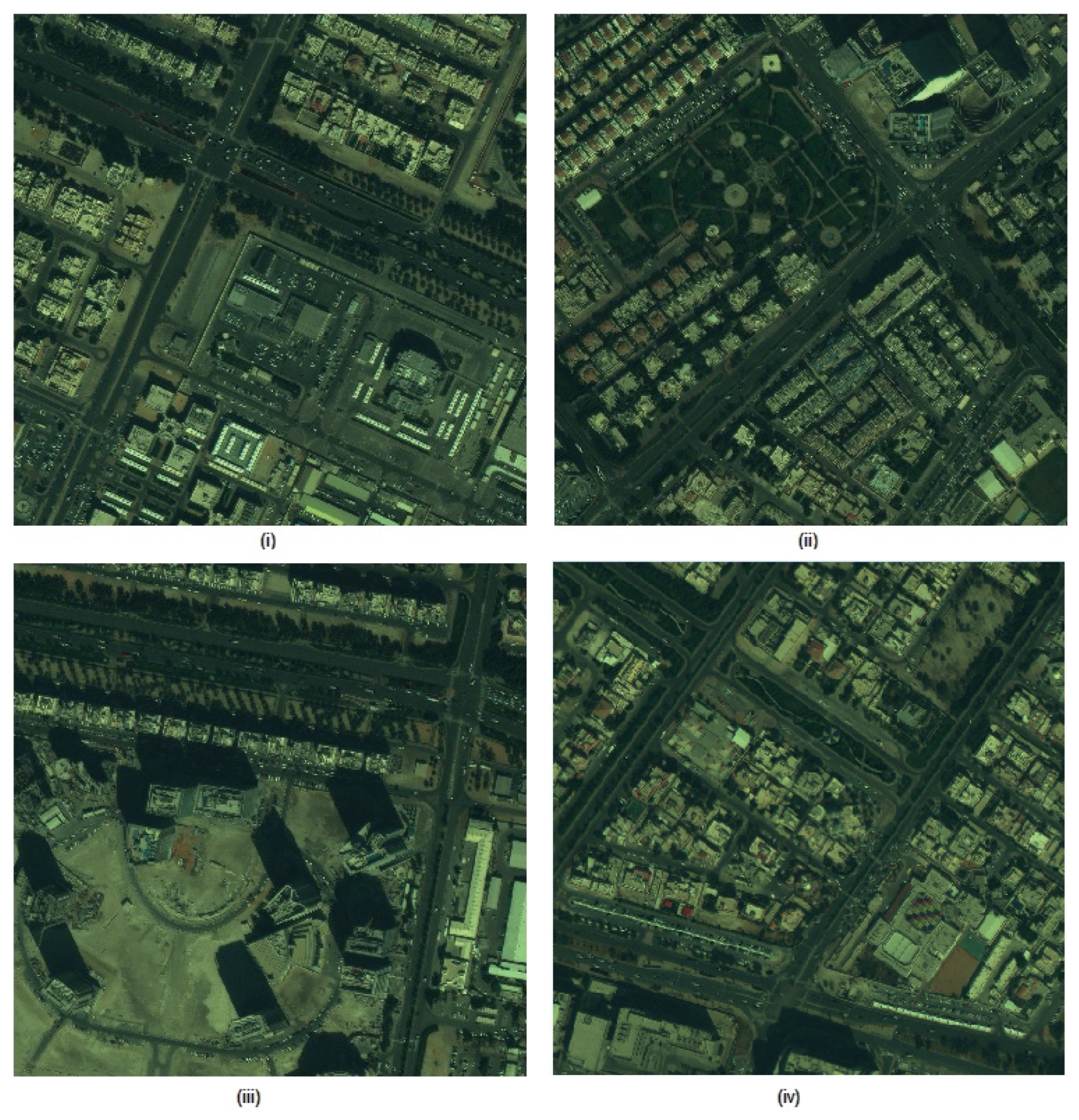
Figure 9.
Output of images from CNN: (i) Image 1, (ii) Image 2, (iii) Image 3, and (iv) Image 4.

Figure 10.
Output of Image 5: (a) CNN Output, (b) Output of VGI overlayed on top of CNN output; pink along with white color indicates VGI output, and (c) Input for post-processing obtained after a removal of VGI output from CNN output.
Figure 10.
Output of Image 5: (a) CNN Output, (b) Output of VGI overlayed on top of CNN output; pink along with white color indicates VGI output, and (c) Input for post-processing obtained after a removal of VGI output from CNN output.
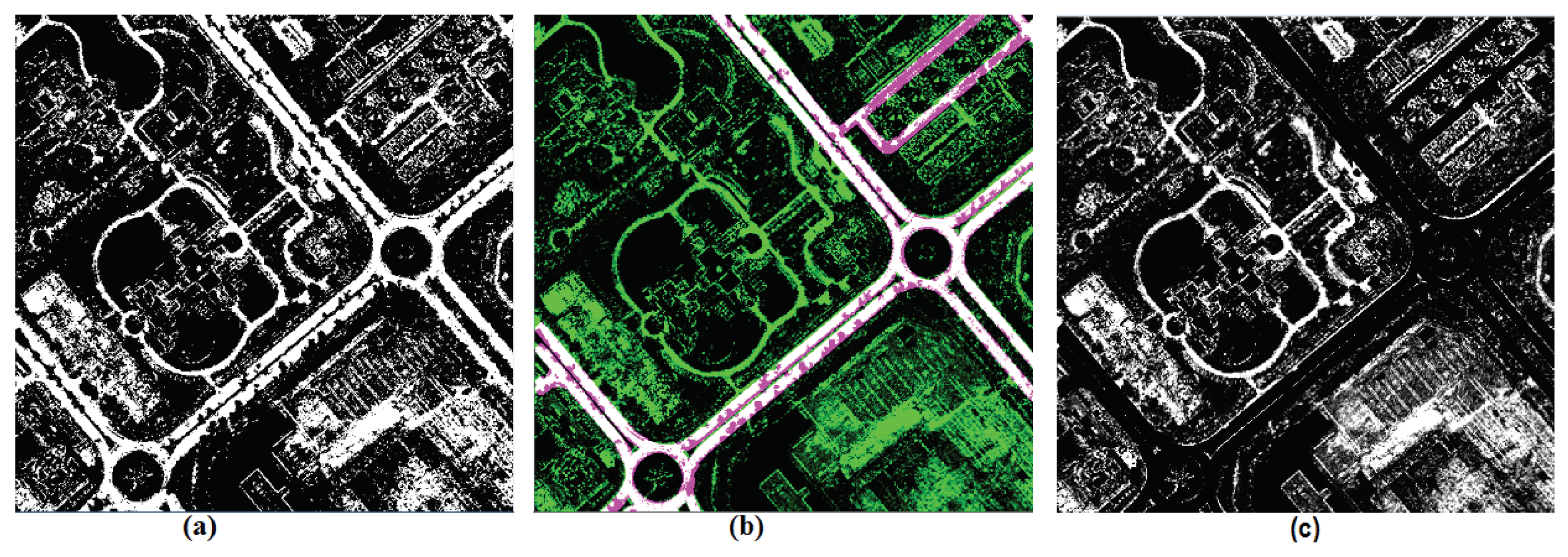
Figure 11.
Branch points in the skeleton of non-road segment samples.

Figure 12.
Branch points in the skeleton of road segment samples.

Figure 13.
Analysis of ratio of the number of branch points to the area of the extracted segment to determine the road segments.
Figure 13.
Analysis of ratio of the number of branch points to the area of the extracted segment to determine the road segments.

Figure 14.
Buildings detected in Image 5 using the segmentation approach [34].
Figure 14.
Buildings detected in Image 5 using the segmentation approach [34].

Figure 15.
Output of Image 5 with removal of vegetation, shadows, and buildings (i.e., after partial post-processing).
Figure 15.
Output of Image 5 with removal of vegetation, shadows, and buildings (i.e., after partial post-processing).

Figure 16.
Output of Image 5 after complete post-processing.

Figure 17.
Output after post-processing in other 4 images: (a) Image 1, (b) Image 2, (c) Image 3, and (d) Image 4.
Figure 17.
Output after post-processing in other 4 images: (a) Image 1, (b) Image 2, (c) Image 3, and (d) Image 4.

Figure 18.
For Image 1: (a) Comparison of output of VGI-only [34] against ground truth (outdated VGI portion highlighted by black oval shape) and (b) Comparison of output of CNN against ground truth.
Figure 18.
For Image 1: (a) Comparison of output of VGI-only [34] against ground truth (outdated VGI portion highlighted by black oval shape) and (b) Comparison of output of CNN against ground truth.

Figure 19.
Comparison of output of CNN against ground truth for: (a) Image 2, (b) Image 5, (c) Image 3, and (d) Image 4.
Figure 19.
Comparison of output of CNN against ground truth for: (a) Image 2, (b) Image 5, (c) Image 3, and (d) Image 4.

Figure 20.
Output of road extraction using the approach of Li et al. [38] with a probability map; (a) Image 1, (b) Image 2, (c) Image 3, and (d) Image 5.
Figure 20.
Output of road extraction using the approach of Li et al. [38] with a probability map; (a) Image 1, (b) Image 2, (c) Image 3, and (d) Image 5.

Figure 21.
(Top) Image 5 with disjoint road segments; (Bottom) Probable nodes in road segments for completing connection.
Figure 21.
(Top) Image 5 with disjoint road segments; (Bottom) Probable nodes in road segments for completing connection.

Figure 22.
Features considered to connect the nodes: (a) Edges detected on Image 5 which acts as noise feature and (b) SLIC segmentation on Image 5.
Figure 22.
Features considered to connect the nodes: (a) Edges detected on Image 5 which acts as noise feature and (b) SLIC segmentation on Image 5.

Figure 23.
Road network formation in Image 5 using feature of distance, segments, and noise: (a) Red line represents probable connection between segments and (b) Road network formation with probable underlying connecting segments.
Figure 23.
Road network formation in Image 5 using feature of distance, segments, and noise: (a) Red line represents probable connection between segments and (b) Road network formation with probable underlying connecting segments.

Figure 24.
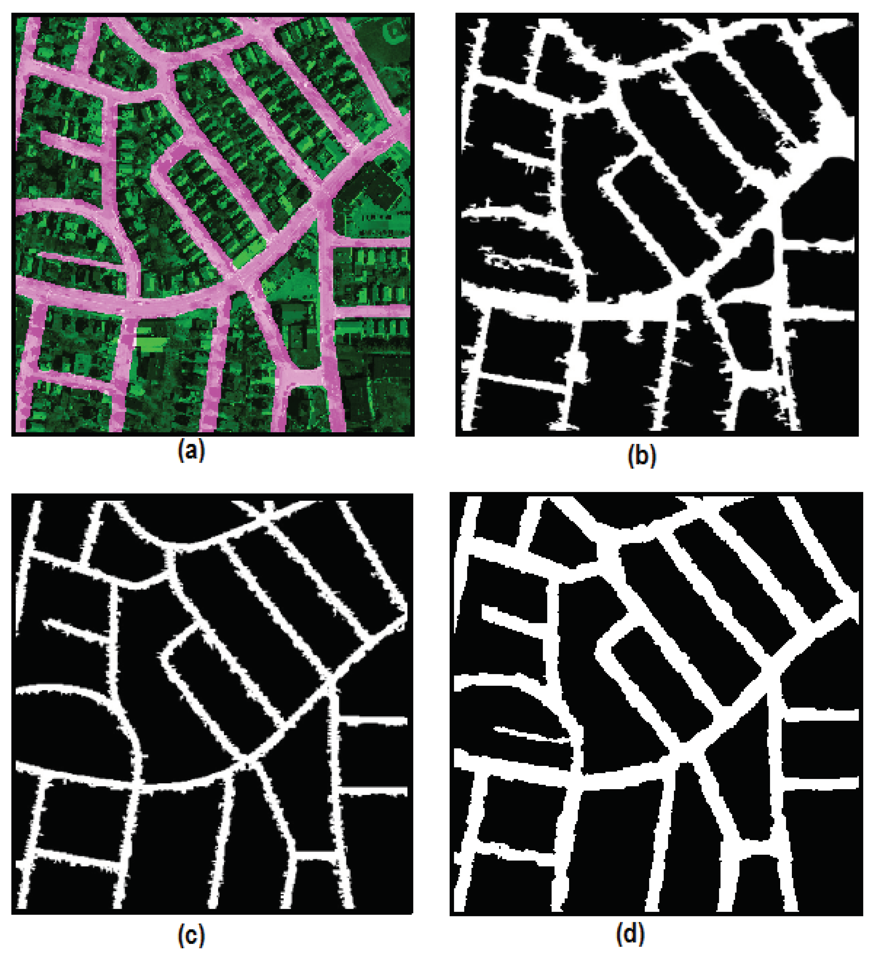
Demonstration in a portion of Massachusetts dataset: (a) Ground truth overlayed on image, (b) Output of VGI approach fed into CNN, (c) CNN results with probable road segments (shown in gray color), and (d) Comparison of output of proposed method (after removal of non-road segments) to ground truth.
Figure 24.
Demonstration in a portion of Massachusetts dataset: (a) Ground truth overlayed on image, (b) Output of VGI approach fed into CNN, (c) CNN results with probable road segments (shown in gray color), and (d) Comparison of output of proposed method (after removal of non-road segments) to ground truth.

Figure 25.
Comparison of outputs: (a) Part of Massachusetts data shown in Fig. with its ground truth, (b) Output using method of Sujatha and Selvathi [39], (c) Output using method of Alshehhi et al. [31], and (d) Output of proposed method.

Table 1.
Performance evaluation in different test images compared to the results of our previous first stage approach [1], i.e., input for CNN against output of proposed approach.
Table 1.
Performance evaluation in different test images compared to the results of our previous first stage approach [1], i.e., input for CNN against output of proposed approach.
| First Stage Output | Output of Proposed Approach | |||||||||
|---|---|---|---|---|---|---|---|---|---|---|
| Measure | Img1 | Img2 | Img3 | Img4 | Img5 | Img1 | Img2 | Img3 | Img4 | Img5 |
| Precision | 0.84 | 0.79 | 0.87 | 0.88 | 0.84 | 0.86 | 0.85 | 0.89 | 0.96 | 0.87 |
| Recall | 0.77 | 0.88 | 0.70 | 0.87 | 0.83 | 0.94 | 0.92 | 0.92 | 0.96 | 0.96 |
| Quality | 0.87 | 0.81 | 0.94 | 0.94 | 0.91 | 0.94 | 0.84 | 0.96 | 0.98 | 0.97 |
| F1-score | 0.81 | 0.83 | 0.88 | 0.90 | 0.85 | 0.88 | 0.87 | 0.90 | 0.95 | 0.91 |
Table 2.
Comparison with other approaches in Abu Dhabi and Massachusetts datasets (** Experiment might have been performed in different images of the same dataset, N/A means data was not reported.).
Table 2.
Comparison with other approaches in Abu Dhabi and Massachusetts datasets (** Experiment might have been performed in different images of the same dataset, N/A means data was not reported.).
| Datasets | Abu Dhabi | Massachusetts | |
|---|---|---|---|
| Methods/Measures | Correctness (%) | Completeness (%) | Correctness (%) |
| Maurya et al. [40] | N/A | 82.3 ± 4.7 | 70.5 ± 4.3 |
| Sujatha and Selvathi [39] | N/A | 83.5 ± 4.3 | 76.6 ± 4.5 |
| Mnih [32] | 78.30 | N/A | 90.1 |
| Shu [41] | 78.2 | N/A | 87.1 |
| Li et al. [38] | 72.25 | N/A | N/A |
| ** Saito et al. [30] | 79.00 | 90.5 | N/A |
| Alshehhi et al. [31] | 80.9 | 92.5 ± 3.2 | 91.7 ± 3.0 |
| Proposed method | 88.61 | 90.8 ± 1.9 | 94.4 ± 3.1 |
© 2019 by the authors. Licensee MDPI, Basel, Switzerland. This article is an open access article distributed under the terms and conditions of the Creative Commons Attribution (CC BY) license (http://creativecommons.org/licenses/by/4.0/).
Share and Cite
MDPI and ACS Style
Manandhar, P.; Marpu, P.R.; Aung, Z.; Melgani, F. Towards Automatic Extraction and Updating of VGI-Based Road Networks Using Deep Learning. Remote Sens. 2019, 11, 1012. https://doi.org/10.3390/rs11091012
AMA Style
Manandhar P, Marpu PR, Aung Z, Melgani F. Towards Automatic Extraction and Updating of VGI-Based Road Networks Using Deep Learning. Remote Sensing. 2019; 11(9):1012. https://doi.org/10.3390/rs11091012
Chicago/Turabian StyleManandhar, Prajowal, Prashanth Reddy Marpu, Zeyar Aung, and Farid Melgani. 2019. "Towards Automatic Extraction and Updating of VGI-Based Road Networks Using Deep Learning" Remote Sensing 11, no. 9: 1012. https://doi.org/10.3390/rs11091012
Note that from the first issue of 2016, this journal uses article numbers instead of page numbers. See further details here.