Comparison of Unsupervised Algorithms for Vineyard Canopy Segmentation from UAV Multispectral Images


1
Institute of Biometeorology (IBIMET), National Research Council (CNR), Via Caproni 8, 50145 Florence, Italy
2
Institute of Clinical Physiology (IFC), National Research Council (CNR), Via Moruzzi 1, 56124 Pisa, Italy
*
Author to whom correspondence should be addressed.
Remote Sens. 2019, 11(9), 1023; https://doi.org/10.3390/rs11091023
Submission received: 9 April 2019
/
Revised: 24 April 2019
/
Accepted: 25 April 2019
/
Published: 30 April 2019
(This article belongs to the Special Issue Remote Sensing for Agroforestry)
Abstract
:Technical resources are currently supporting and enhancing the ability of precision agriculture techniques in crop management. The accuracy of prescription maps is a key aspect to ensure a fast and targeted intervention. In this context, remote sensing acquisition by unmanned aerial vehicles (UAV) is one of the most advanced platforms to collect imagery of the field. Besides the imagery acquisition, canopy segmentation among soil, plants and shadows is another practical and technical aspect that must be fast and precise to ensure a targeted intervention. In this paper, algorithms to be applied to UAV imagery are proposed according to the sensor used that could either be visible spectral or multispectral. These algorithms, called HSV-based (Hue, Saturation, Value), DEM (Digital Elevation Model) and K-means, are unsupervised, i.e., they perform canopy segmentation without human support. They were tested and compared in three different scenarios obtained from two vineyards over two years, 2017 and 2018 for RGB (Red-Green-Blue) and NRG (Near Infrared-Red-Green) imagery. Particular attention is given to the unsupervised ability of these algorithms to identify vines in these different acquisition conditions. This ability is quantified by the introduction of over- and under- estimation indexes, which are the algorithm’s ability to over-estimate or under-estimate vine canopies. For RGB imagery, the HSV-based algorithms consistently over-estimate vines, and never under-estimate them. The k-means and DEM method have a similar trend of under-estimation. While for NRG imagery, the HSV is the more stable algorithm and the DEM model slightly over-estimates the vines. HSV-based algorithms and the DEM algorithm have comparable computation time. The k-means algorithm increases computational demand as the quality of the DEM decreases. The algorithms developed can isolate canopy vegetation data, which is useful information about the current vineyard state, and can be used as a tool to be efficiently applied in the crop management procedure within precision viticulture applications.
1. Introduction
The use of precision agriculture is spreading thanks to the increasing capabilities of modern technologies [1,2]. The goal is to optimize agronomic inputs with the aim of increasing sustainability, yield and quality of the production. As a consequence, the correct use of these technologies reduces the overall cost of agronomic management. The main techniques used to monitor crop development are based on proximal and remote sensing approaches. Remote sensing consists of the acquisition of crop information via satellite, aircraft or Unmanned Aerial Vehicle (UAV) platforms [3,4]. In particular, the latter permits a low altitude flight survey for the provision of maps with high spatial resolution [5,6,7]. Precision viticulture (PV) is a branch of precision agriculture that investigates the vineyard spatial variability, which directly affects grape yield and quality [8]. In the last decade, UAV platforms have been increasingly used due to the high spatial resolution achieved but also the extreme flexibility and promptness in field survey scheduling. Photogrammetric processing of imagery, as point cloud(s), is used to compute orthomosaics, Digital Elevation Models (DEM), and 3D models of the monitored area [9].
UAV can be equipped with a wide range of imaging sensors useful to reliably describe the spatial variability in vineyards. RGB and multispectral cameras are the most frequently used sensors in precision viticulture applications [10]. RGB acquires spectral bands not only in the visible (Red-Green-Blue (RGB)) and multispectral but also in the near infrared spectrum (Near infrared-Red-Green (NRG)). For example, multispectral remotely sensed images in the near infrared are helpful to characterize the crop vegetative status through computation of spectral indices, such as the widely used Normalized Difference Vegetation Index (NDVI) [11]. The NDVI correlates with biomass, photosynthetic activity and, sometimes, with grape quality properties [12,13,14,15].
The main difference between traditional platforms and UAV is the ground sampling distance (GSD), which is the mean distance associated with a pixel in an image, and the data acquisition frequency. UAV-based acquisition can reach very low GSD, however, a finer GSD does not mean that the “image quality” is good enough to correctly identify different elements of a vineyard, such as vines, bare soil, weeds and shadows. Pruning, weather and light exposure are all aspects that may affect the acquisition, and neighbouring pixels can present a similar spectral response even if they should represent soil or canopy [16]. The distinction among vines, bare soil, weeds and shadows is a key point to efficiently monitor a vineyard [5,17].
Supervised methods are nowadays often used to extrapolate vegetative information, even if they are time consuming, error-prone processes and stressful for the user [16,18]. The traditional approach is to develop a graphical user interface, which enables the user to assign a category to each pixel by clicking on it or selecting a determined area. Other methodologies are based on a thresholding approach of the color distribution, through commercial programs such as Matlab, ImageJ or similar [19,20]. Unsupervised methods are currently also being developed because they assure in-line identification of plants in the field and a faster delivery of results than a supervised method [17,21,22]. Machine learning unsupervised clustering algorithms, such as the k-means algorithm [23], are used for this.
The common steps performed in a threshold method are to define subsequent masks by selecting predefined ranges or color layers composing an image. The threshold value, or interval, is selected by the user, observing the color distribution, or by automatic techniques. Otsu’s technique is often used as an automatic thresholding method in precision viticulture and, generally, in image segmentation [22]. Otsu’s thresholding technique clusters the image pixels into two classes, foreground and background, by computing a color threshold from the selected channel. Otsu’s method works on the color distribution or indices distribution even if these acquisitions are made with different cameras. This step may induce co-registration errors and then a misleading identification of plants [24]. To avoid these errors, Gebhardt et al. converted the RGB images into grayscale, generating local homogeneity images to detect a homogeneity threshold [25]. The main limitation of threshold techniques is stability of the binarization accuracy of the system, as any mis-segmentation is generally caused by an error in the detected threshold. So, if the detected threshold is not appropriately estimated, the generated segmentation process will be strongly affected. Another issue is related to the effect of light conditions on the vegetation segmentation results achieved, particularly in sunny and overcast conditions [20].
Different color spaces may be used instead of the RGB one, to overcome the unwanted light effects. The HSV (Hue, Saturation, Value) and L*a*b* color spaces are widely used to isolate green elements in an outdoors image. For example, the k-means algorithm is applied on the L*a*b* color space since it is distance-based, increasing the capabilities of this clustering method. The research by Calvario et al. on agave control is a good example of the ability of UAV mixing computer vision and data mining technique in precision agriculture [26].
Another example is the LABFVC algorithm proposed by Liu [19]. Passing by the L*a*b* color space, the Fractional Vegetation Cover (FVC) is extracted automatically. Instead of distinguishing on color value, the LABFVC isolates vegetation and soil from their color distributions, which are supposed to be Gaussian. More recently, Song proposed a shadow-resistant version, postulating the SHAR-LABFVC algorithm on the shadow distribution [20].
Intra-row vegetation, i.e., weeds or similar, generates a series of issues in vines identification, since it modifies both the color distribution and vineyard geometry. Bobillet proposed an unsupervised algorithm to cluster vine rows based on vineyards’ active contours [27]. However, these unsupervised approaches require a more complex structure of the code, with a structured decision tree. For example, the OBIA (Object-based Image Analysis) procedure proposed by de Castro [21] is robust and fully automatic, applying local filters to the DEM. A similar approach has been proposed by Padua [28], where multi-spectral descriptive indices are also adopted to overcome issues related to the identification of vines. Finally, the simplest way to isolate vines from a DEM is to retrieve the Canopy Height Model (CHM), obtained subtracting the Digital Terrain Model (DTM) from the DEM. The DTM can also be estimated by the DEM [29]. The DEM model gives consistent information about the physical characteristics of the field, such as biomass [30,31,32,33]. Also, from this model, it is possible to correctly identify vines when the bare soil elevation is known, which is sometimes trivial to retrieve but, in other cases, requires considerable supervised work.
The aim of this paper is to propose fast unsupervised segmentation algorithms, developed in Matlab 2016 [34], to be applied on RGB or NRG orthomosaics. For both RGB and NRG orthomosaics, two algorithms are proposed recursively applying Otsu’s thresholding technique to each channel composing the image. The Hue-Saturation-Value (HSV) color space is always used as intermediate color space, because of its ability to classify color frequencies with respect to saturation and chromatic values [24]. The other two algorithms are the k-means, which is commonly used in precision agriculture, and an algorithm for the DEM model that does not involve DTM computation. Three different scenarios are chosen to compare these algorithms. The focus of the comparison is the ability of these algorithms to over- and under-estimate vines in cases where the DEM is not accurate, paying attention to the computational resources required. Moreover, attention will be given to the computational time of the identification.
The paper is structured as follows. Methodologies are introduced in Section 2: technologies related to remote sensing (UAV and payload), and numerical algorithms to isolate vines in RGB and NRG mosaics. In Section 3, the tests scenarios are briefly described and then the comparison is illustrated separately for RGB and NRG orthomosaics. The discussion of this comparison is addressed in Section 4. Lastly, Section 5 reports the conclusions and future directions towards new unsupervised methods.
2. Materials and Methods
This section describes the methodology used in this work. Firstly, the remote sensing platform in three different scenarios is introduced, along with the software used to generate the mosaic of each vineyard. Unsupervised algorithms to isolate vines on RGB and NRG images are then presented. Lastly, the method used for comparison is described.
2.1. UAV Remote Sensing Platform and Dataset
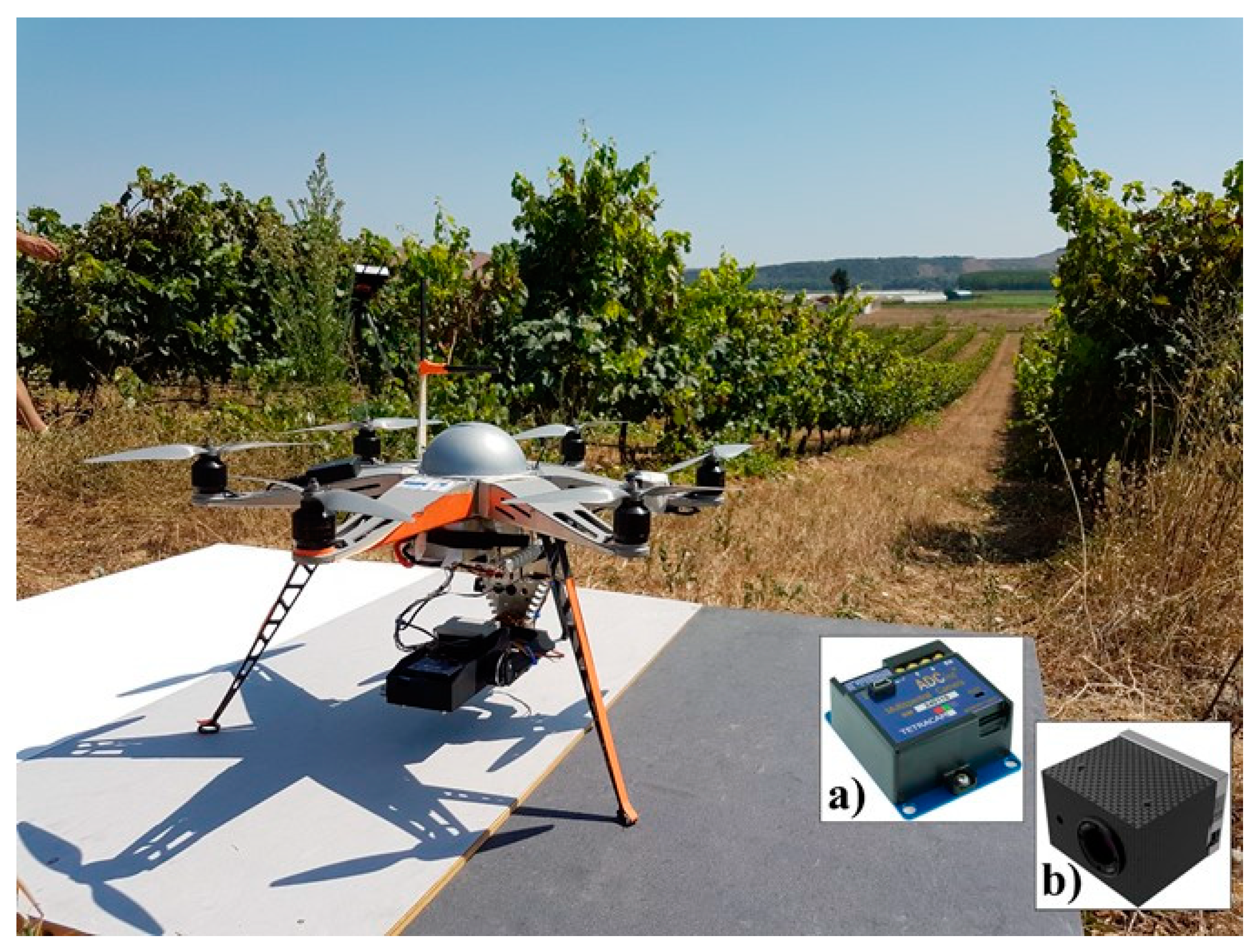
Flight campaigns were conducted using an open source UAV platform (Figure 1) that consists of a modified multi-rotor Mikrokopter (HiSystems GmbH, Moomerland, Germany). An on-board navigation system assures autonomous flight through a pre-imposed set of waypoints, selected via the Mikrokopter Tool software (V2.20 HiSystems GmbH, Moomerland, Germany). The flight control unit (Mikrokopter Flight Controller ME V2.1, HiSystems GmbH, Moomerland, Germany) controls six brushless motors, assuring the correct route by communicating with a GPS module (U-blox LEA-6S, U-blox AG, Thalwil, Switzerland) and a navigation board (Navy-Ctrl 2.0, HiSystems GmbH, Moomerland, Germany). UAV flight was controlled using a ground station, ensuring real-time image acquisition at 5.8 GHz via a WiFi module (Mikrokopter, HiSystems GmbH, Moomerland, Germany). Maximum payload is approximately 1 kg, ensuring 15 min of operating time with one 4 S battery at 11000 mAh.
The UAV payload, shown in Figure 1, consisted of two different cameras to acquire multispectral images in both the visible and infrared spectra. For the acquisition in the infrared spectrum, a Tetracam ADC Snap multispectral camera (Tetracam, Inc., Gainesville, FL, USA) was used to collect the Near Infrared band (NIR) along with the Red and Green bands in the visible spectrum (Figure 1a). The output of the Tetracam is a three-layer image, i.e., an NRG (NIR-Red-Green) acquisition.
To collect the visible spectrum, a ThermalCapture FUSION was used (Figure 1b). This is a dual camera, especially designed for small UAVs, which stores radiometric thermal images as well as 2 MP RGB images, fully aligned to improve thermal analysis performance. In this paper, only a three-layer RGB image was used to evaluate the proposed methodologies’ potential on low resolution images considering other RGB cameras available on the market.
Table 1 summarizes the main characteristics of the cameras. Each one has a different Field Of View (FOV), which is a critical aspect in flight planning, directly related to the degree of overlap.
Images were mosaicked using Agisoft Photoscan Professional Edition 1.4.3 (Agisoft LLC, St. Petersburg, Russia) [35]. Agisoft first produces a polygon mesh and then the dense 3D point cloud. At this point, the pixel values of each image are projected onto the mesh to create an orthomosaic. When combined with the GPS positions, this process allows the creation of a high-resolution orthophoto and the DEM of the experimental site [29]. DEMs are obtained using RGB and NRG sensors separately using Agisoft Photoscan without ground control points, with only GPS data of each image using Agisoft capability to perform alignment autonomously. Point cloud density obtained was 11 points/cm2 for NRG and 19 points/cm2 for RGB, respectively. Agisoft performs DEM using IDW (Inverse Distance Weighted) interpolation.
In this paper, three different remotely sensed scenarios were selected to compare algorithms, considering both RGB and NRG acquisitions during the same flight.
The same flight plan was used for all the surveys, adapting it to maintain the same UAV flying height of 50 meters above the ground at a speed of 2.5 m/s and time of flight around 12:30 p.m. In this way, the mosaics are expected to have a comparable ground resolution. The sampling time of both cameras was set to have 70% of forward overlap and the distance between flight lines was set to ensure 70% of lateral overlap.
The first scenario refers to a remote sensing survey on 7 July 2018, of a 1 ha commercial vineyard (Tenuta Pernice) in Piacenza (Italy) (44°58′47.6″N, 9°25′44.0″E), labeled as V1. A Barbera cv. vines (Vitis vinifera L.) vineyard was planted in 2004 with NE-SW rows orientation and spacing of about 2.1 m × 1.5 m (inter-row and intra-row). The vineyard is located on a slight west-southern slope at 355 m above sea level. The sky was clear, there was no rain on the previous day and average temperature was about 35 °C. This scenario is labeled as P18.
The other two scenarios refer to a 1.4 ha commercial vineyard (Castello di Fonterutoli–Marchesi Mazzei SpA.) in Castellina in Chianti (Siena, Italy) (43°25′45.30″N, 11°17′17.92″E), labeled as V2. Sangiovese cv. vines (Vitis vinifera L.) were planted in 2008 on a slight southern slope at 355 m above sea level, with 2.20 m × 0.75 m vine spacing and NW-SE rows orientation. Vines are trained to a vertical shoot-positioned trellis and spur-pruned single cordon with four two-bud spurs per vine. At this site, two flight surveys were performed in two different years: 9 August 2017, scenario labeled as M17, and 8 August 2018, labeled as M18. In M17 scenario, vine pruning and removal of grass cover between rows was performed just before the flight. In M18 scenario, the same management was planned a couple of days after the flight. Weather conditions were also completely different. The 2017 season was extremely hot and dry compared to the 2018 one, consequently, canopy development in 2017 was exceptionally low.
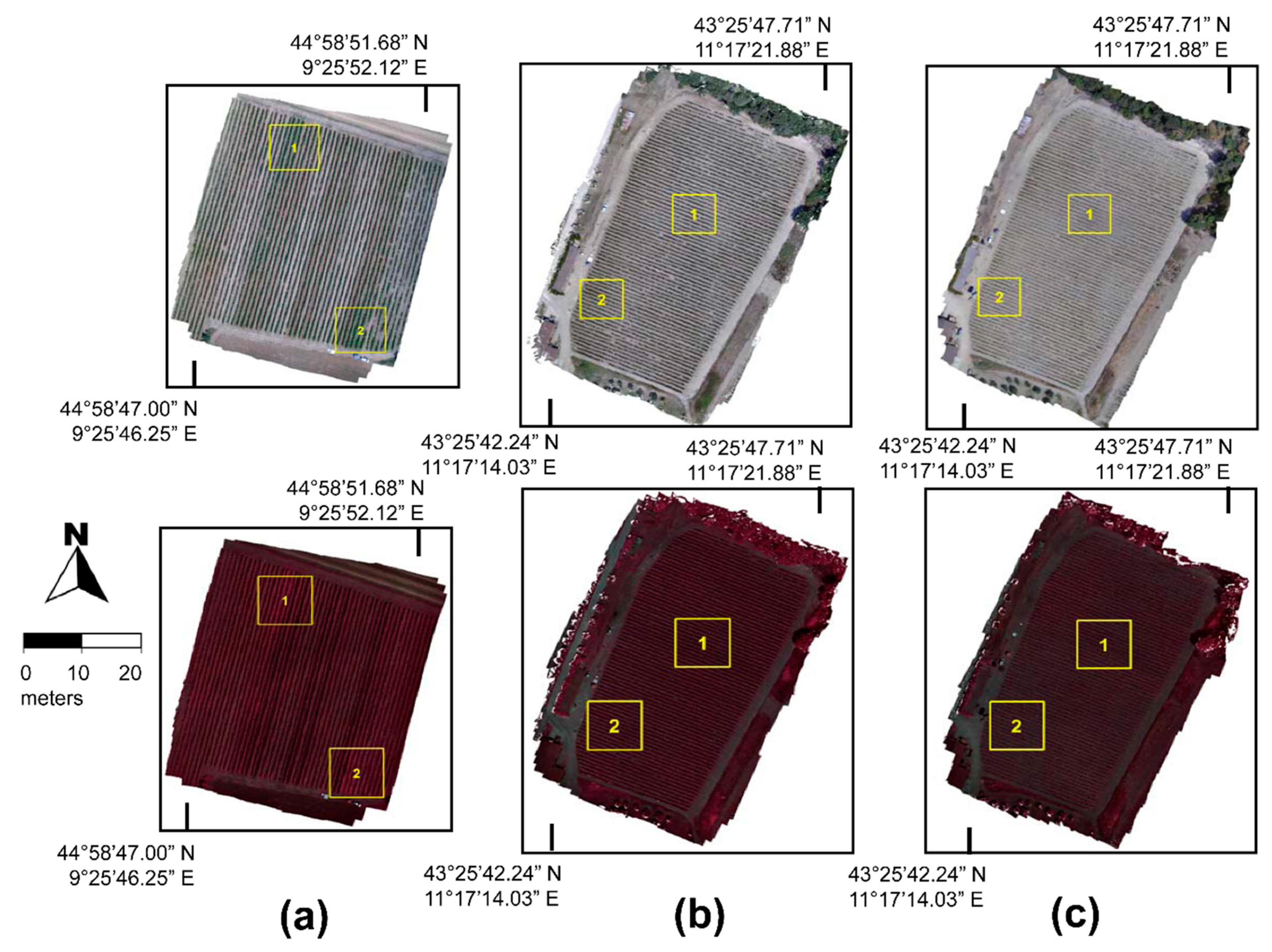
These three scenarios differ by the DEM features, as illustrated in Figure 2. An aerial image of vineyard V1 is shown in Figure 2a. A similar image of vineyard V2 is shown in Figure 2b, taken during the 2018 flight survey. In both images it is possible to distinguish the geometrical characteristics of the vineyards.
A similar view of the images in Figure 2a,b is then shown for the DEMs obtained from both RGB and NRG mosaics. The P18 scenario, Figure 2c, has a regular and well-defined DEM, for both RGB and NRG acquisitions. Comparing Figure 2c with Figure 2a, it is possible to conclude that both DEMs approximate the main vineyard features well, i.e., intra-row distance, vines height and thickness.
The quality of the DEM decreases consistently for the M18 and M17 scenarios, see Figure 2d,e respectively. The DEM obtained from the NRG acquisition of M18 scenario is quite accurate (Figure 2c), even if some particulars are different. See, for example, the vines on the upper left corner of the image, under the tree. The DEM obtained from the RGB acquisition is able to detect the intra-row distance between vines. However, many computational vine gaps are present with some local peaks. Vine height also appears to be under-estimated from the model.
The vineyard features are completely lost in the M17 scenario. Both RGB and NRG DEMs are almost flat, with some local peaks. No reliable information can be obtained from these DEMs regarding the vineyard features.
The three scenarios show different features of the DEM model even if the pixel resolution is similar, about 0.03 × 0.03 m. It is possible to conclude that the P18 scenario has the more accurate DEM. The M18 is of intermediate quality and, for the M17 scenario, the quality is very poor.
2.2. Unsupervised Methods for RGB Images
This sub-section presents the unsupervised algorithms used to identify vines from RGB images. The visual camera assigns to each pixel a value of the primary colors Red, Green and Blue, i.e., an RGB image. This trichromy is additive: this means that secondary colors are generated by the summing of three values corresponding to each pixel. The main elements noticeable from an RGB image of a vineyard are soil, shadow, weeds and vines. In this approximation, soil refers to bare soil and weeds together.
This paper proposes the first two algorithms, based on the features of the HSV color spectrum. The HSV trichomy is not additive since a color is represented in cylindrical coordinates in the HSV color space. The other two algorithms, k-means and DEM algorithms, have been utilized in previous studies and are used here as batch solution for the HSV-based algorithms. All the algorithms are developed using MATLAB (version 2016, MathWorks Inc., Massachusetts, USA) [34].
2.2.1. Soil, Shadow and Canopy Filtering Passing by HSV Spectra
All steps of the two unsupervised algorithms to isolate vines from RGB images are now described. These two algorithms identify soil, shadow and vines by color thresholding, using the HSV color spectrum. The HSV color spectrum assigns to each spectral frequency, identified by the value of hue (H), a chromatic saturation magnitude (S, where 0 is white and 1 is full color) and value (V, where 0 is black and 1 is full color). The spatial representation of the HSV color space is a cone, with H as angular reference, considering the red primary frequency at 0°, passing through the green primary frequency at 120° and the blue primary frequency at 240°. In this color space, having fixed the color frequency, the effect of light with respect to shadows is prominent and vice-versa.
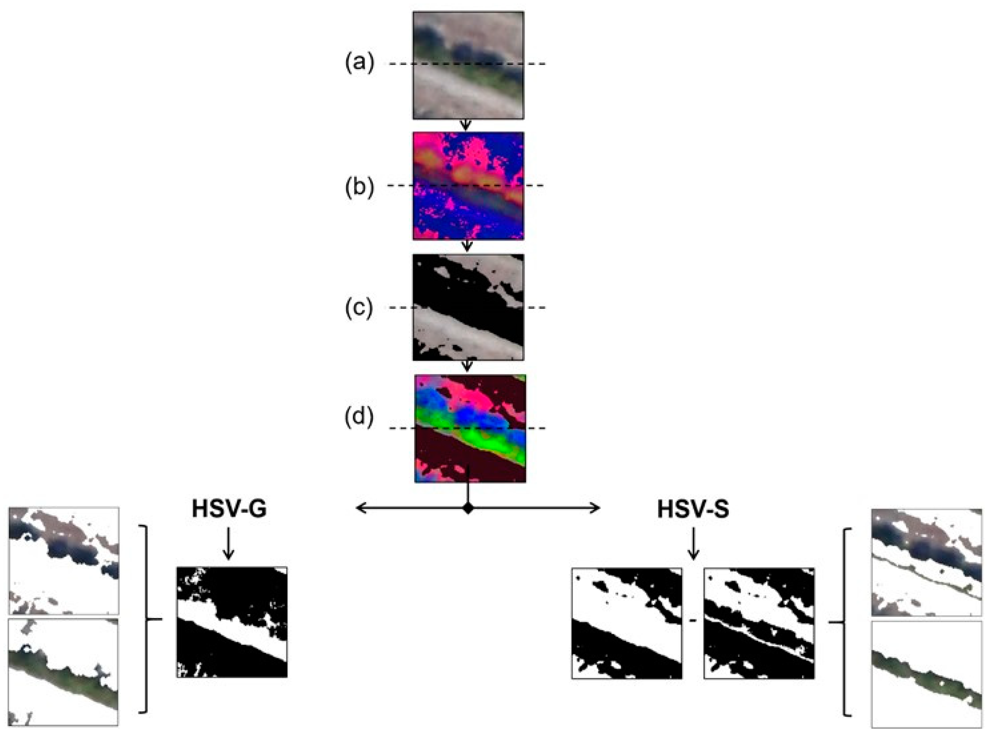
The workflow of the HSV-Green and HSV-Shadow algorithms, namely HSV-G and HSV-S, are reported in Figure 3. The main steps are consistent with some classical supervised methods, i.e., they isolate vines by creating a series of subsequent masks by color thresholding. The proposed HSV-G and HSV-S algorithms have the same workflow, which differs only in the last part.
Both algorithms start from the RGB image (Figure 3a) that is converted into the HSV color spectrum (Figure 3b). At this point, see Figure 3b, it is possible to notice that soil is almost identified by the blue color. The representation in Figure 3b is additive, the same as that used for RGB images. Then, exploiting the analogy within the RGB color space and the HSV color space, soil is extracted from the Value (V) layer. From an operational standpoint, soil is identified taking only pixels that have a magnitude of V greater than the threshold reference obtained through Otsu’s thresholding technique. The mask thus obtained is applied to the RGB image and soil is presented in Figure 3c.
The complementary mask of the one shown in Figure 3c contains vines and shadows. The high contrast format of this complementary RGB image is presented in Figure 3d. This image is obtained with the “decorrstretch” function in Matlab 2016. Before this conversion to the high contrast format, all the pixels identifying soil are converted to black. This step is useful to emphasize the difference between shadows and vines applying Otsu’s thresholding technique on the next step, forcing the color distribution.
After this (Figure 3d), the HSV-G and HSV-S algorithms differ in how the vines are identified. The HSV-G algorithm extracts green pixels from the mask obtained at the aforementioned intermediate step. The HSV-G algorithm extracts the mask identifying vines obtained from Figure 3c, without soil, applying Otsu’s thresholding technique to the high contrast green layer. Only pixels with higher green content are retained. The HSV-G algorithm lastly identifies shadows by subtracting soil and vine masks from the complete image.
The HSV-S algorithm proceeds the other way around from the HSV-G, first segregating shadows and then extracting vines from the complete image. The HSV-S extracts the mask identifying shadows, considering a composite mask from the blue and red layer. This mask is obtained considering pixels that have a blue value less than Otsu’s threshold applied to the blue channel or pixels that have a value of red less than 10. This value is retrieved from Figure 3d, selecting all visible low red pixels. The HSV-S algorithm identifies vines by subtracting the shadow mask from the complementary mask identified in Figure 3c.
2.2.2. K-Means Algorithm for RGB Images
The k-means segmentation method is an unsupervised approach often used in pattern recognition problems. The k-means method is used to identify and separate plants from soil and weeds; these different classes are identified in the image with a distance criterion, thanks to a pointwise similarity function or equalizing the variance of families in these layers. The idea is to segregate k similar families of pixels (clusters) with a similar function, which is usually the mean value of the associated function (e.g., pixel value).
The first step is to convert the RGB image into the CIE-L*a*b* format [20] to emphasize the capabilities of the k-means method. In the L*a*b* color space, colors are seen in a spatial distribution line of Luminance (L*), green-red line (a*) and yellow-blue distribution line (b*). On these lines it is possible to visualize the amount of red/green or blue/yellow in an image, pixel by pixel. For example, a value of a* < 0 refers to green chromatic intensity while a* > 0 refers to red chromatic intensity. The same goes for b* in the blue/yellow color line. The conversion from RGB to L*a*b* is done in Matlab 2016 by the corresponding function, using the “d65” reference white that simulates the not exposed colors.
K-means parameter was imposed to identify k = 5 clusters [26,28,36], considering the mean value of pixels in both the a* and b* channels. The k-means segregates clusters considering their mean value. So, the cluster with the lower value of a*, i.e., strongest intensity of green, is identified as vines. On the same line, the shadows cluster is selected as the one with positive value of a* and lower value of b*. The remaining three clusters identify soil.
2.3. Unsupervised Methods for NRG Images
The NRG multispectral camera assigns, to each pixel, a value of Near-infrared (NIR), Red and Green. The additive super-imposition of these frequencies determines a particular image, which we named NRG for simplicity. It is possible to visualize an NRG image by the “false-color” technique. The following algorithm was developed to isolate soil, shadow and vines separately following a similar approach to the HSV-S for RGB images.
2.3.1. Soil, Shadow and Canopy Filtering Passing by HSV Spectra
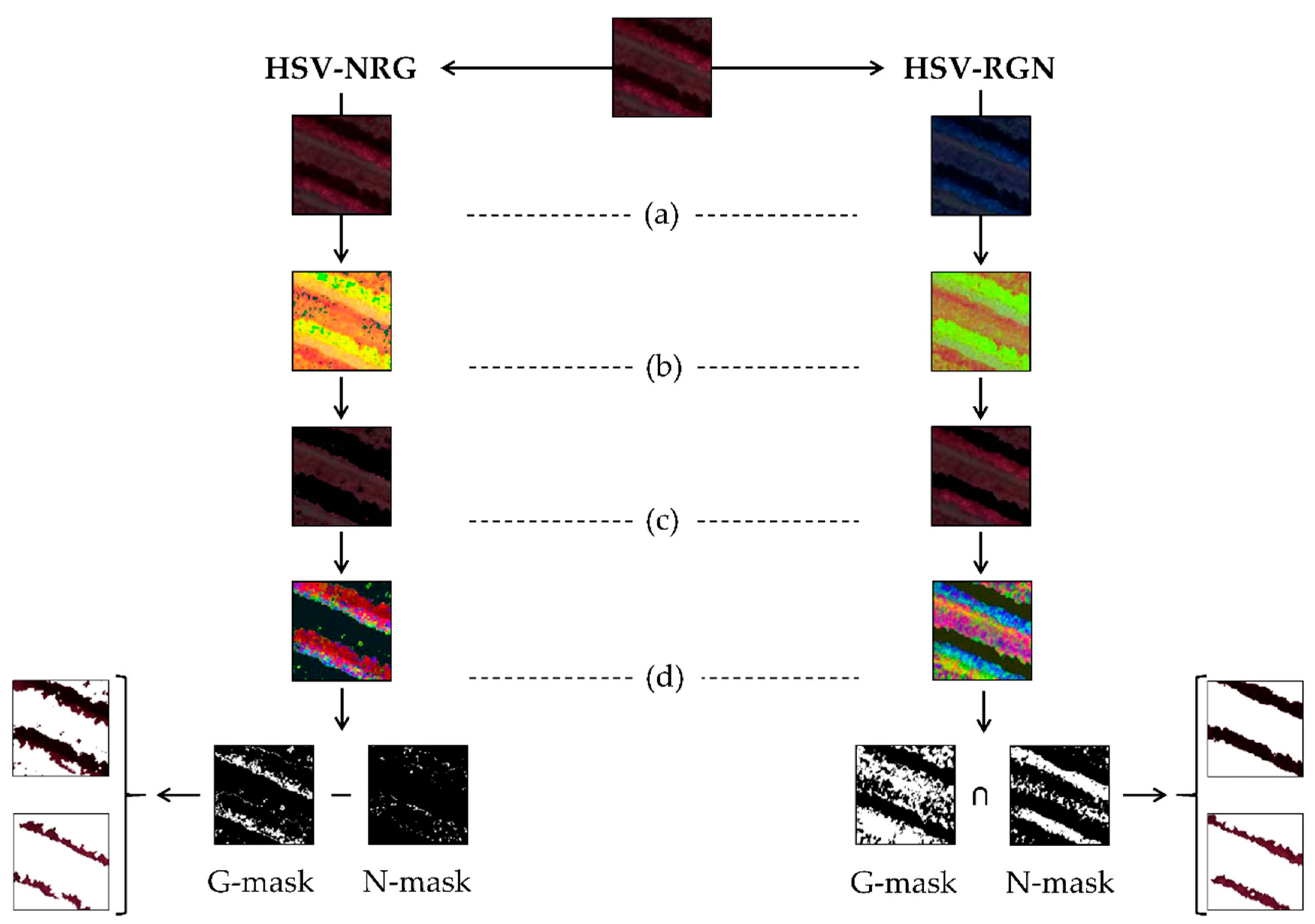
Two unsupervised algorithms were developed for NRG images, the HSV-NRG and HSV-RGN. HSV-NRG and HSV-RGN workflows are reported in Figure 4 for an easier visualization of all the proposed steps.
The HSV-NRG directly converts the image to the HSV color space, see Figure 4a for HSV-NRG. The saturation channel (S) is used to identify shadows, retaining pixels with a higher value of Otsu’s threshold. This is shown in Figure 4c for HSV-NRG. The non-shadowed image is then turned at high resolution with the “decorrstretch” function in Matlab 2016. Starting from Figure 4d for HSV-NRG, vines are then identified from the non-shadowed image as follows. A first mask is obtained selecting pixels with the higher content of G, applying Otsu’s threshold to the overall distribution (G-mask) and this set of pixels is converted to black. The N channel is then considered, computing Otsu’s threshold and retaining pixels with a lower magnitude that are retained (N-mask). HSV-NRG at this point identifies soil by subtracting the shadow and vine masks from the complete image. The remaining set of pixels is vines.
The HSV-RGN proceeds in a similar way to the HSV-NRG but changing the orders of layers before converting the image to the HSV color space. From the NIR-Red-Green layering, the image structure changes to Red-Green-NIR. The channel tricomy is similar to an RGB image but with Nir instead of blue, see Figure 4b for HSV-RGN. In this way, the image conversion to HSV color space gives a different final output, see Figure 4b for HSV-NRG. At this point, the filtering on the S channel is done, as with the HSV-NRG, to segregate shadows from the overall image. This non-shadowed image is turned at high resolution with the “decorrstretch” function in Matlab 2016. As in the HSV-NRG, the G-mask and N-mask are obtained but, in this case, from the high-resolution image obtained with the “decorrstretch” function in Matlab 2016. Vines are isolated by considering the common positive pixels of the G-mask and N-mask. The final step is to identify soil by subtracting the shadow and vine masks from the complete image.
Figure 4a shows the difference of the visualized image inverting the three layers from NRG to RGN. The output of the color stretching is visible in Figure 4b, exploiting the different boundary distinction between the two formats. Figure 4c,d show the segmentation of soil (shadow for the RGN algorithm) and the stretching of the remaining colors that leads to the final step of each algorithm.
2.3.2. K-Means Algorithm for NRG Images
K-means algorithms were also applied for NRG images and the same approach as the RGB image imposing k = 3 clusters was used. However, in this case, the a* channel does not represent the green-red distribution line, but the NIR-green one. The cluster with higher green content, which has the maximum value of a*, is identified as vine. From the two remaining channels, the cluster with lower luminance (L) is identified as shadows.
For the sake of explanation, the k-means algorithm considering the RGN format of the images was also tested. In this way, the L*a*b* conversion returns the a* channel representing the green-red color space, without modifying the transformation matrix. K-means algorithm for the RGN image was applied without satisfactory results. Anyhow, these topics require further investigation in future research.
2.4. Unsupervised Methods for DEM Model
The DEM model consists in a matrix of local coordinates associated with vineyard height and representing its morphology. The vines were isolated directly from the digital image instead of computing the Digital Terrain Model (DTM). The isolation of vines is easier by passing by the DTM since they are obtained by subtracting the DTM from the DEM. However, calculating a DTM requires interpolation and thus introduces inaccuracies.
A geometrical top-hat filtering is applied to the DEM by using the “imtophat” function in Matlab. The closure shape chosen is an ellipse of 2 × 1 pixels. The DEM is converted to binarized images where the bare soil is somewhat flat and Otsu’s threshold is then applied to separate the foreground, vines, from the background, soil and shadows. Following this method, it is not possible to identify shadows in the image.
2.5. Comparison Methodology
A typical machine learning technique, the contingency table, is used in this paper to compare the ability of algorithms to isolate vines. A contingency table is defined in machine learning/predictive control to validate if the learned/predicted dataset is in accordance with a reference one. The contingency table is a confusion matrix if data are learned/predicted from a supervised method, as in our case. Instead, the contingency table is a matching matrix if data are learned/predicted from an unsupervised method.
After the identification step by an unsupervised algorithm, the contingency matrix is computed by comparing the single-pixel category of the algorithm, pixel by pixel, to the single-pixel category obtained from a supervised method. A Graphical User Interface (GUI) is then implemented in Matlab 2016 to compute the contingency table for each of these sub-zones. This interface allows us to select each pixel, or a cluster of them, assigning the corresponding category to it/them.
In machine learning, generally, the accuracy of an algorithm is measured by summing up all the pixels predicted correctly by the unsupervised algorithms, to obtain a more compact visualization of results. The accuracy is computed summing all the elements in the main diagonal, divided by the total number of pixels composing the image. This approach has often been used in precision agriculture, when there is the need to validate an identification algorithm [5,20,21,36].
However, there is a drawback regarding the data analysis related to how the accuracy matrix is defined. For example, in an RGB image of a vineyard, three possible categories are visible: soil (considering also weeds), shadows and vines. In this work, these three categories are used to classify the results of each algorithm. The accuracy of an algorithm is merely the sum of all the well-identified categories that are, considering a contingency table, the elements on the main diagonal. See, for example, Poblete et al. [16] and Padua et al. [5]. However, by computing the accuracy in this way, it is not possible to extrapolate the information if one of these categories is estimated correctly, which is the main goal of this work. For this reason, two indices are defined to quantify if the algorithm used over-estimated and/or under-estimated a chosen category.
The contingency matrix assigned the first row/column to the category “Soil”, the second row/column to “Shadow”, and the third to “Vines”. The results of the supervised algorithm are stored in the rows (reference dataset) and those from the unsupervised algorithm are stored in the column. The accuracy of the algorithm is therefore the sum of the main diagonal, i.e., . The element defines the number of pixels identified by the supervised algorithm that are soil. The same applies to and with shadow and vines.
Let us consider only the category vines. The real number of pixels identifying vines is the sum of all the elements on the third row, . On the contrary, the total number of pixels identified as vines by the algorithm is the sum of all the elements on the third row, . So, the sum of elements and , gives the total number of pixels missed as vines by the algorithm, which are identified as soil () and shadow (). Similarly, the sum of elements and gives the total number of pixels identified as vines by the algorithm but that are not vines in reality. These pixels are soil () and shadow ().
Following the observation, the over-estimation index is , which is the sum of pixels that are vines, but not identified as such, by the real number of pixels identified as vines. The over-estimation index indicates how much an algorithm over-estimates vines. Similarly, the under-estimation index is , which is the sum of pixels incorrectly identified as vines. The under-estimation index indicates how much an algorithm under-estimates vines. These indexes can be extended to soil and shadow by selecting the corresponding elements.
3. Results
This section compares the ability of different unsupervised algorithms to isolate vines from shadows and soil in an RGB and NRG image. The results are presented distinguishing the comparison between the RGB and NRG image types. Firstly, the three scenarios (P18, M18, M17) are briefly discussed, exploiting the different features of the orthomosaics. At this point a visual comparison of all algorithms is addressed. Finally, the under- and/or over-estimation indices are presented considering the application of each algorithm to the complete mosaic or sub-regions of 1000 × 1000 pixels.
All the computational analyses presented in this paper were performed in the workstation available at IBIMET Firenze. This workstation has 2 processors, Genuine Intel(R) CPU 0000 @ 2.40GHz with 14 Cores and 28 Threads each and 256 GB of RAM. The video card is a NVIDIA Quadro M6000 with 24 GB of dedicated RAM. We also used this workstation to build the mosaic and the DEM in each selected scenario.
3.1. Algorithm Comparison: From the Test Scenarios to Data Analysis
Three scenarios were selected (P18, M18 and M17) to compare algorithms, presenting different features on the final orthomosaic and the DEM model in Figure 2. These three scenarios are from two different sites where remote sensing was conducted using the methodology described in Section 2, which also presented the flight plan and vineyard features. Both RGB and NRG orthomosaics for the three scenarios are introduced in Figure 5.
Visually, the P18 orthomosaic clearly shows a regular order of the vineyard, and in some zones it is easy to distinguish between soil and vines. Comparing the RGB and NRG images, there is no evident difference. However, in some zones, there are a lot of weeds. Grassing could induce an error in all the RGB and NRG algorithms. Also, the presence of missing plants is more pronounced in the lower part of the site. The two sub-regions are then selected for the effect of grassing and missing plants in the identification.
The same observations hold for the Mazzei vineyard in Castellina in Chianti. However, the M18 and M17 scenarios have a different definition of boundaries among vines, soil and shadows. In 2017, the flight took place after vine harvesting and a de-grassing operation. This operation was done after the acquisition in 2018. The M17 orthomosaic shows the less accurate definition of the vineyard in both NRG and RGB images, with a lower quality of the DEM.
To complete the presentation of the three scenarios, Table 2 reports their dimensions in terms of horizontal and vertical number of pixels and ground sampling distance (GSD), which is the physical distance associated to each pixel. The three scenarios P18, M18, M17, were selected because they are also comparable in terms of resolution.
The P18-1 zone is now considered in Figure 6. Figure 6a presents the real result of P18-1 zone, showing the RGB images with the associated category. Five square sub-regions of 128 × 128 pixels have been defined and they are shown by white squares. Here, the categories are identified and reported as percentage of the total number of pixels (128*128 = 16384) in the neighbouring bar plot. Figure 6b presents the result of the segmentation via the k-means unsupervised algorithm. The same five squares of 128 × 128 pixels have been considered and used to compute the confusion matrix. The central sub-region, labeled as “E”, is considered in Figure 6b as representative example.
It is important to note that, as highlighted in Section 2.5, the sum of each row gives the results of Figure 6a and the sum of each column is coincident with the result of Figure 6b. The accuracy of the algorithm in identifying soil (elements in main diagonal) is 0.28, shadow is 0.20 and vines is 0.20. The total accuracy of the k-means algorithm, is therefore 0.68. However, as explained in Section 2.5, this number does not give any information about the consistency of this accuracy. For example, let us consider a generic algorithm that is not able to identify vines and defines all the remaining set of pixels as shadow and soil. The accuracy of this algorithm would be, at maximum, 0.72, i.e., the total number of real pixels that are soil and shadow. This accuracy is greater than the k-means value that gives a reliable representation of the field, noticeably comparing Figure 6a,b. In this case, no information is given on how the algorithm under-estimates vines. Instead, let us imagine the results of an algorithm that identifies the entire field as vines. The accuracy is then 0.28. However, in this case, no information is given on how much the algorithm over-estimates vines.
Thus, in this paper, the over-estimation indexes defined in Section 2.5 are introduced to determine the algorithm ability in the segmentation. These indexes, in machine learning, are also known as true-positive and false-negative indexes.
The over-estimation index of soil is : this means that the algorithm tends to under-estimate vines because of its under-estimation index is . In the case of soil, the over estimation index is and the under estimation index is . The algorithm tends to over-estimate soil at the expense of vines estimation.
This approach is then repeated for all five squares, computing the over- and under-estimation index of the considered algorithm. The mean value between the over-estimation index and under-estimation index is then computed independently, considering the latter as negative. If this mean value is positive, the algorithm tends to over-estimate vines. Instead, a negative value of this index indicates that the algorithm tends to under-estimate vines. This procedure is extended to each zone of every orthomosaic, for each algorithm proposed and used in the following to compare the algorithms through different scenarios.
3.2. Unsupervised Methods Applied to RGB Images
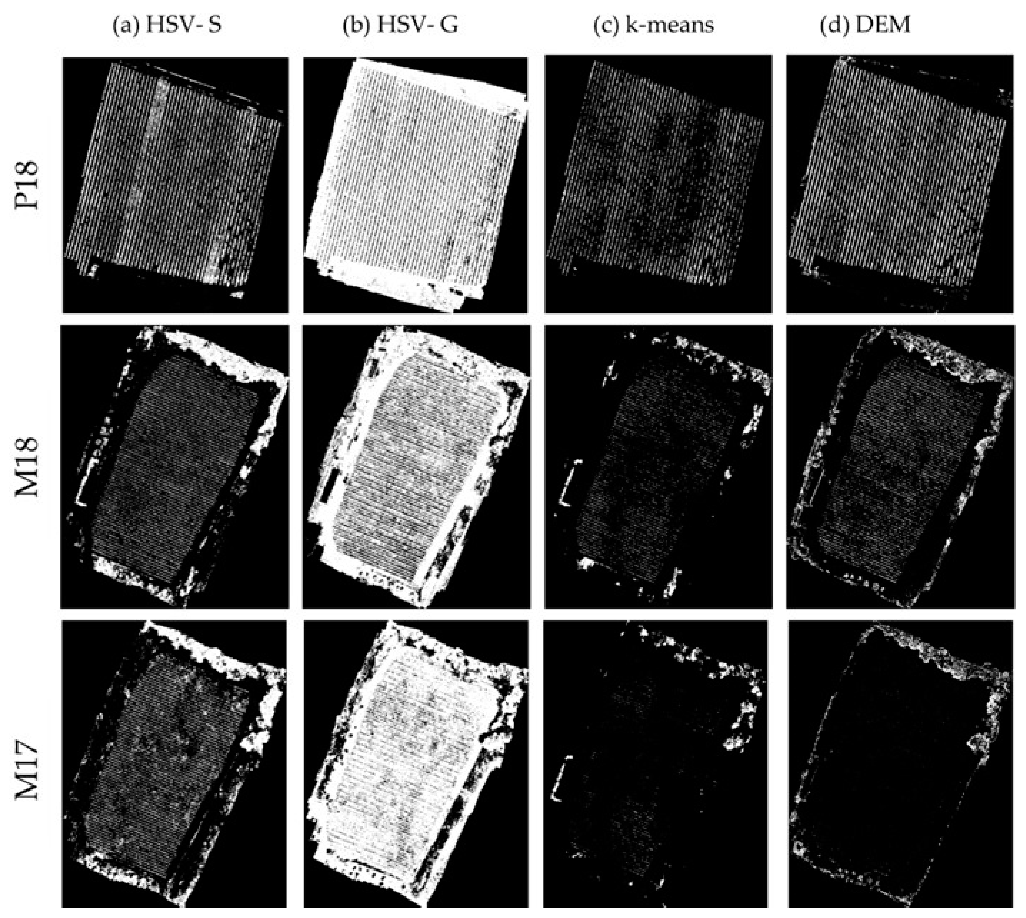
All algorithms were applied to the complete orthomosaics, obtaining a binary mask identifying vines. Results are shown in Figure 7. Non-vineyard vegetation is present in the imagery such as trees along with bad photogrammetric processing present in the borders of the orthophoto mosaics. This vegetation has been maintained to stress the performance of algorithms, but this interaction will not be considered in real-usage scenarios. Visually, comparing this mask to Figure 7, the results obtained via the DEM model seem to be the more accurate. Also, the HSV-S shows a regular representation of the rows and, for the M17 scenario, gives the more reliable approximation of the vine rows where the DEM model fails to do so. On the other hand, the K-means seems to under-estimate vines and the HSV-G clearly over-estimates them.
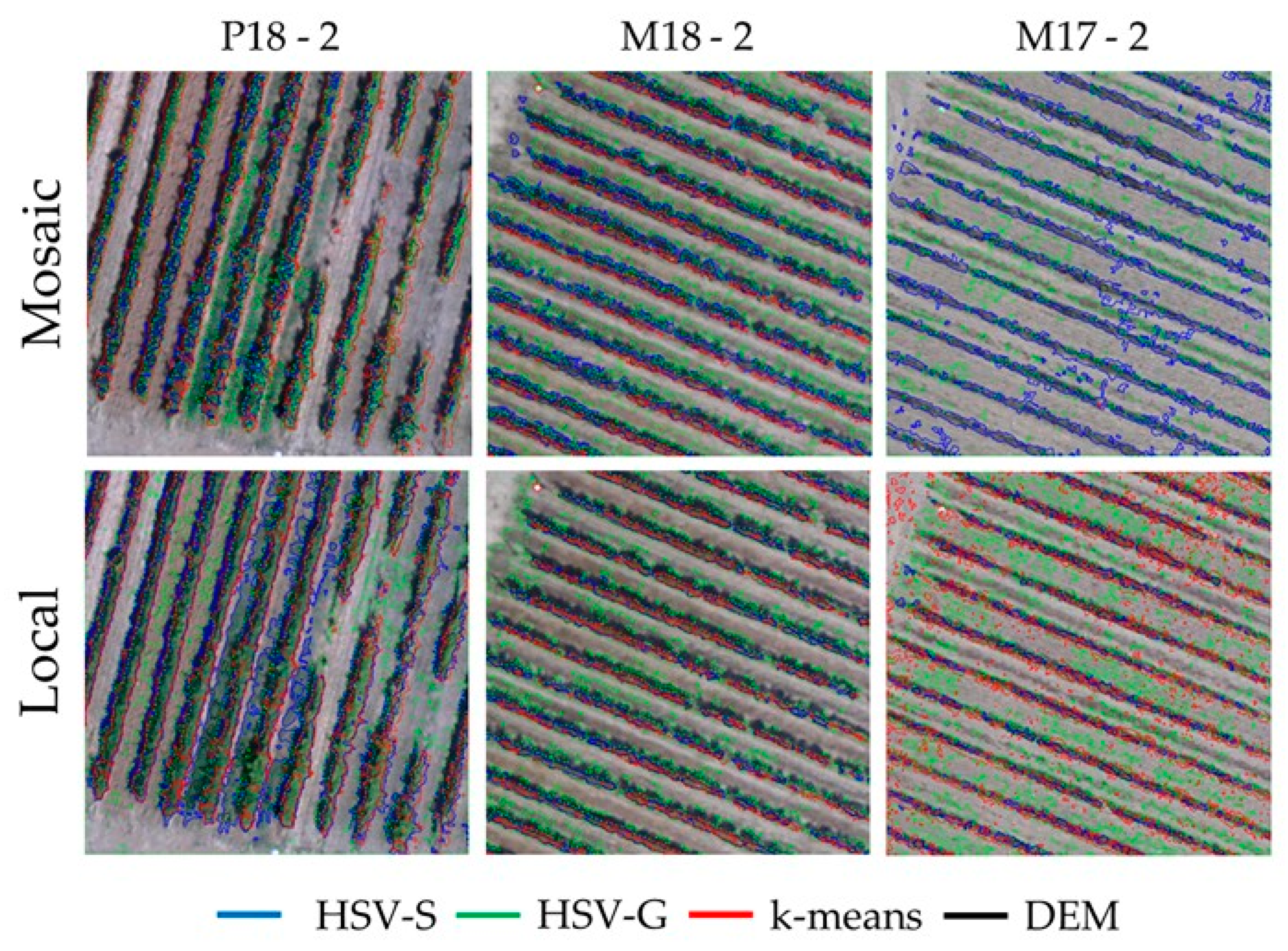
All algorithms are then applied locally in the sub-regions shown in Figure 6, obtaining also, in this case, masks identifying vines. A visual comparison of the results is shown in Figure 8, in terms of boundaries of each mask, represented by different colors. The blue line is for the HSV-S, green for the HSV-G, red for the K-means algorithm and black for the DEM model.
The vine boundaries obtained via the DEM model, as expected, do not change considering the local and global application of the various algorithms. However, the DEM’s ability to isolate vines is strictly dependent on its quality. It is possible to clearly see that the vine boundaries in M17 are indistinct, as it is almost flat.
Moving to the other algorithms, the HSV-G seems to be the least accurate. It also isolates weeds (P18 orthomosaic and local) and parts of the soil (M18 orthomosaic and local). A different scenario is noticeable for the HSV-S algorithm. It can identify vines, but is sometimes unable to distinguish between soil, shadows and canopy. However, if it is applied locally, it performs well also in the case of the M17 site, where both the k-means and DEM algorithms fail.
The k-means algorithm is visually the most accurate for the P18 and M18 sites. It can isolate vines, shadows and soil almost correctly in these cases. In addition, it is able to not include weeds when it is applied locally, even if it misses vines (see lower part of the P18-local image). However, for the M17 site, its ability to identify vines decreases substantially. For its local applications, the results seem to be better but it is not completely clear what the k-means algorithm is able to isolate.
At this point, the over- and under-estimation indices are presented in Figure 9, assigning a different color to each scenario, and distinguishing between (a) orthomosaic and (b) local application of the algorithm.
The results are in accordance with what was observed before. The HSV-G consistently over-estimates vines, never under-estimating them. The k-means and DEM method have a similar trend of under-estimation regarding the orthomosaic application, which may depend on the clarity of the image in distinguishing vines and soil/shadow. In addition, it is possible to approximate an error of 15-20% for the DEM, see orthomosaic application on P18 (Figure 9), which depends on the average presence of shadows in the image. The k-means tends to under-estimate vines, but it has the best identification performance for the RGB images. The HSV-S over-estimates vines if it is applied to the orthomosaic. However, it gives the best approximation of vines in its local application, under-estimating them.
The computational times to obtain the results presented so far are shown in Table 3. The HSV-S and HSV-G algorithms have comparable computational times, since they work in a couple of subsequent steps where binary masks are computed and summed up/subtracted together. This also explains why the HSV-G is always the faster algorithm, as it is structured with the fewest intermediate steps.
The DEM algorithm identifies vines in a comparable time to the HSV-S and HSV-G algorithms. However, the computational time necessary to build the DEM from the orthomosaic is substantial.
Finally, the k-means algorithm increases the computational demand as the orthomosaic quality decreases. Also, we noticed that the k-means decreases the computational time in M18-Z1, M17-Z1 and M17-Z2 sub-regions where its ability to identify vines also decreases.
3.3. Unsupervised Methods Applied to NRG Images
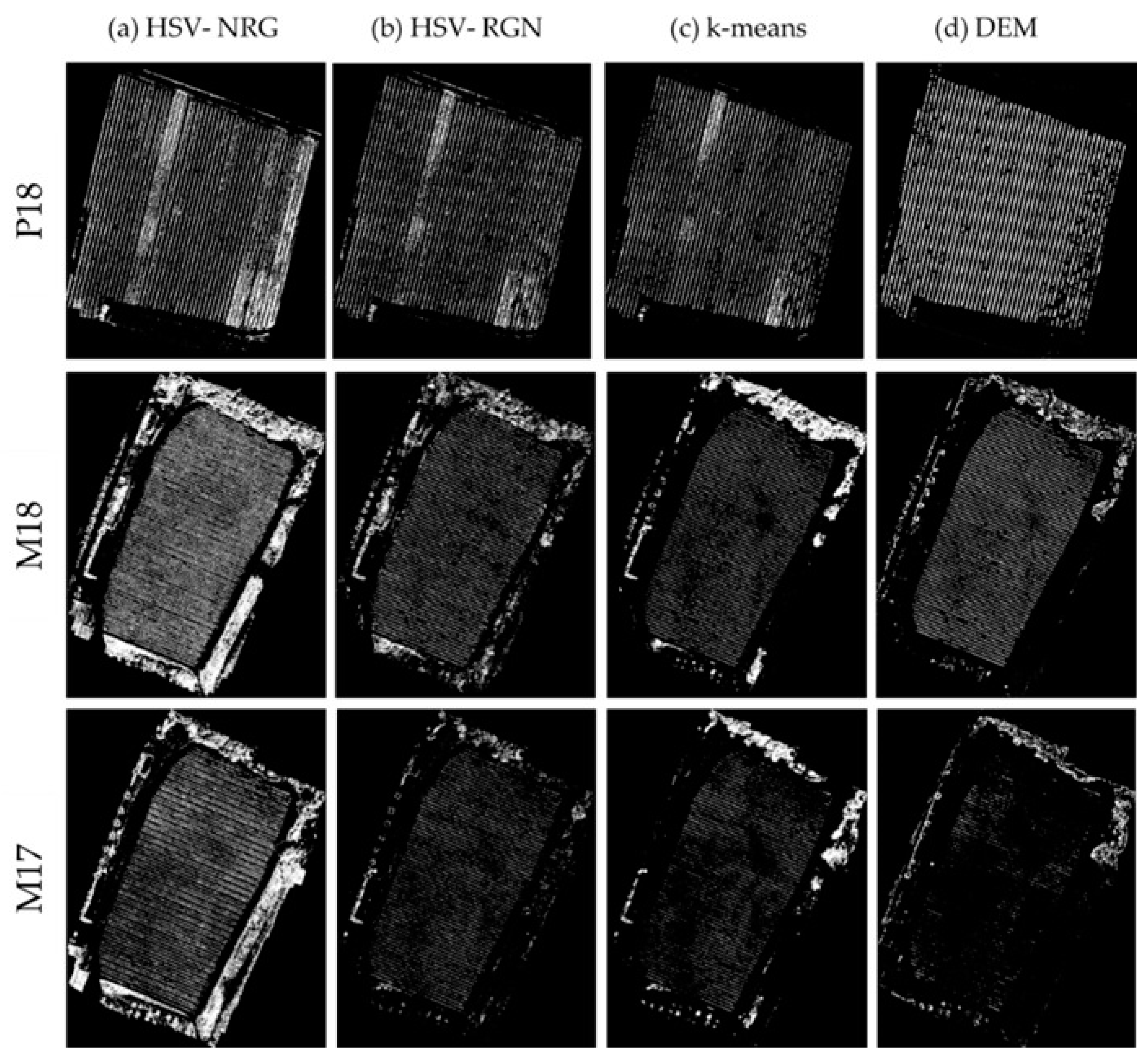
The focus is now on the NRG acquisitions. This type of acquisition is important as it gives information about some important indices used in precision agriculture, such as the NDVI. Figure 10 shows the binary masks representing vines for all the unsupervised algorithms in NRG orthomosaics.
The identification ability of the DEM model decreases drastically with its quality. For the NRG image, it is possible to note that, even when the quality of the image decreases, all algorithms show a considerable ability to identify the vineyard pattern. The HSV-RGN algorithm seems to be the most precise in the identification. The k-means suffers in the M18-1 and M17-1 sub-regions, which are the same but taken in different conditions; this also happened for the RGB image, see Figure 6. The HSV-NRG seems to over-estimate vines and, in some cases, identifies weeds as vines.
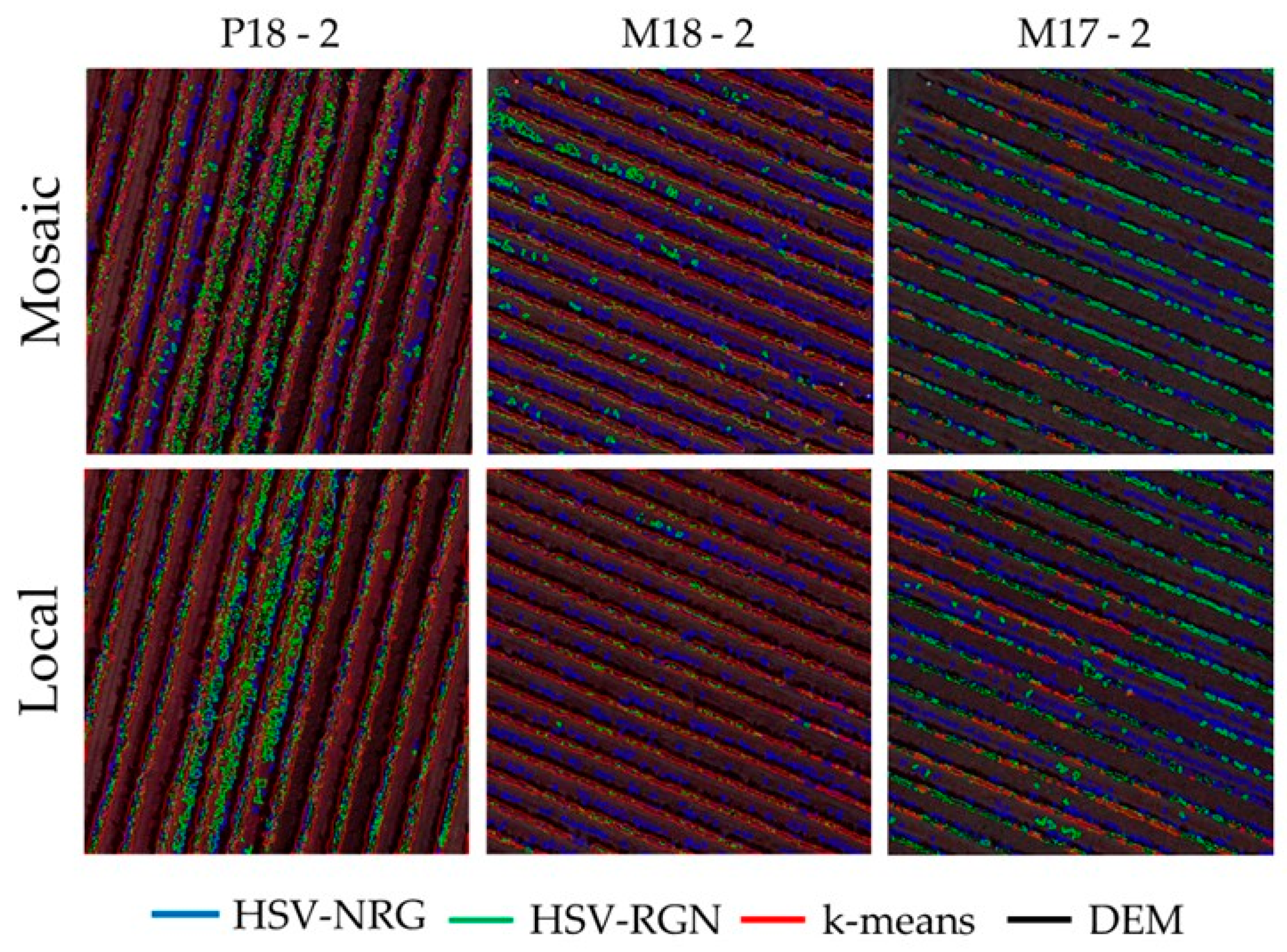
Figure 11 shows the visual comparison of NRG algorithms, confirming the observations made for the orthomosaic application. It shows the local masks signed as 1 in Figure 6, which could be the most complex area where there are a lot of weeds. In fact, The HSV-RGN method, even if it correctly identifies all the vine boundaries, over-estimates them because it also identifies weeds as vines. Instead, the k-means algorithm in some cases over-estimates vines as the line is far from the vine boundary, but it is more effective in not considering weeds as vines.
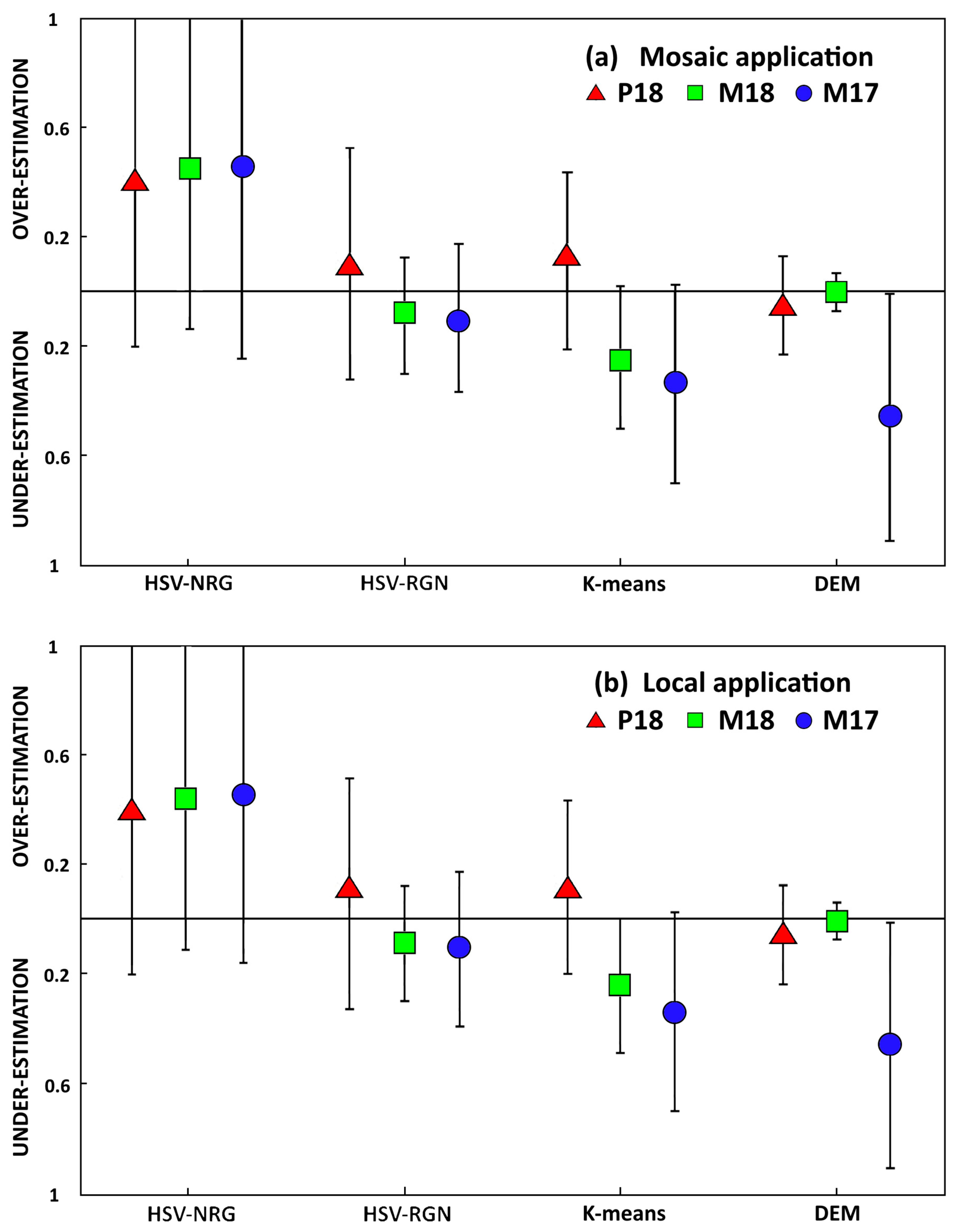
The over- and under-estimation indices are now presented in Figure 12 for the NRG scenarios. Also, in this case, the average value of each index between the two sub-regions of each site is considered. No major difference is observed comparing the orthomosaic and local application. The HSV-RGN is the more stable algorithm. The k-means has no increment of performance passing from the orthomosaic to local application, contrary to what is observed in the RGB image. In this case, the DEM model slightly over-estimates the vines in all cases and it provides almost perfect identification of the M18 site.
Lastly, the computational times required for NRG images are given in Table 4. The same trend is observed as that for the RGB acquisitions. HSV based algorithms and the DEM algorithm have comparable computation time. The k-means algorithm increases the computational demand as the quality of the DEM decreases, but it reduces the computational time in the cases where it performs less well, such as the M17-Z1 and M17-Z2 sites. This time reduction is not very marked as for the RGB images. The same holds for the identification ability of the k-means between RGB and NRG images. In the case of RGB images, k-means reduced its identification ability whereas, for NRG images, this reduction is mitigated.
4. Discussion
Regarding RGB acquisitions, the k-means algorithm is the more stable over the identification in the orthomosaic and sub-regions. It has a very good ability to not over-estimate vines in each condition but, when the quality of the image decreases, it substantially under-estimates vines, as in the case of the M17 scenario.
Both HSV-based algorithms have opposite performances. The HSV-G over-estimates vines when it is applied to the orthomosaic because it is focused on the total distribution of green on the field. Local application of the HSV-G mitigates its over-estimation trend.
The HSV-S algorithm markedly over-estimates when it is applied to the orthomosaic. Instead, when it is applied locally it behaves in the opposite way. Moreover, the magnitude of the over- and under-estimations is more limited. The HSV-S performances are comparable to the k-means algorithm and, in some scenarios, it provides a better approximation of vines as for the M17-1 sub-region. From the orthomosaic to the local application, the only consistent difference is the color distribution. The local value of the pixel is the same but the color distribution alters significantly, changing the capabilities of Otsu’s technique to identify the correct color threshold value. Therefore, further investigation will involve the color distribution and its thresholding technique, also considering methods based on a statistical distribution as done by Liu for the LABFVC algorithm [19].
If the NRG acquisitions are considered, none of the algorithms proposed show a different behavior between their orthomosaic and local applications. The differences are small (less than 5% of error) and they mainly concern identification of weeds in the field. This lack of difference needs further investigation to clarify it, considering other scenarios and different color distributions.
The HSV-RGN algorithm is the more stable over the identification in the orthomosaic and sub-regions. Its performances are comparable to those of the k-means. The k-means under-estimates vines in a marked way and, only for the P18 scenario, its over-estimation of vines is consistent. In the other scenarios, it maintains its quality in a slight over-estimation of vines, as observed for the RGB images.
The paper of Calvario et al. [26] follows a similar approach on agave plants, but only applies the k-means algorithm on the cultivation. The main approaches pursued so far have a more complex decision tree, passing through different steps to isolate canopy, in this case vines. For example, both Poblete et al. [16] and Padua et al. [5] were able to accurately find vines in a complex image by interpolating the results of various intermediate masks. Both studies used either DEM data or the 2G_RB index. The 2G_RB index is obtained, pixel by pixel, by summing 2 times the value of the green pixel and subtracting the value of the blue and red layer. This index is also discussed, highlighting the importance of the green pixel value with respect to shadows. Here, it is found that the blue layer is important to separate soil from vines and shadows.
The OBIA algorithm proposed by de Castro et al. [21] is surely the most accurate and effective one developed so far. It is able to isolate vines by means of a series of intermediate steps considering both geometrical observation, DEM and color intensity. With the OBIA algorithm, it is also possible to identify missing plants and compute biomass.
Bobillet et al. [27] presented an image processing algorithm for automatic row detection using an active contour model consisting of a network of lines to adjust to the vine rows.
Kalisperakis et al. [31] estimated canopy levels from hyperspectral data, 2D RGB orthomosaics and 3D crop surface models found good correlation (r2 >73%) with the ground truth.
Burgos et al. [32] have used a differential digital model (DDM) of a vineyard to obtain vine pixels, by selecting all pixels with an elevation higher than 50 cm above the ground level showing good results. A manually delineation of polygons based on the RGB image was used to obtain those results.
Weiss and Baret [33] have used the terrain altitude extracted from the dense point cloud to get the 2D distribution of height of the vineyard. By applying a threshold on the height, the rows were separated from the row spacing. The comparison with ground measurements showed RMSE = 9.8 cm for row height, RMSE = 8.7 cm for row width and RMSE = 7 cm for row spacing.
However, all these methods require a very good quality of the DEM, which is the focus of this paper. When it is inaccurate, it is not possible to distinguish between the various components in the image and other approaches are required.
Finally, to the knowledge of the authors, no identification approach has been proposed and discussed for NRG images. The purpose of this paper is to introduce this discussion and, certainly, the related investigation and procedure will be discussed and improved to achieve a precise identification of vines, to produce accurate descriptive maps (NDVI for example) of the entire field.
However, the simulation performed here shows that the k-means algorithm is demanding computational times at least 10 times greater than the HSV-based algorithms. This is a strong limitation if the final aim is the in-line use of the k-means algorithm for real time identification, as in the case of unsupervised UAV to autonomously monitor vineyards or crop fields.
These observations certainly drive future research into the development of more accurate unsupervised HSV methods. The proposed algorithms can be improved by following other methods, such as the loss of color distribution, studying a different method from Otsu’s one to define the distribution threshold, or simply by combining the already existing methods. A thorough study of the band included in the filtering will also help in the definition of the correct payload to be mounted in the UAV platform.
This suggests a study about the k-means algorithm workflow, to reduce its computational time. The clustering ability of the k-means method is strictly connected to the computational time necessary. As this increases, it also increases its identification ability of vines. A deeper investigation into this aspect may highlight the bottlenecks of this algorithm, suggesting some modification or perhaps the use of parts of this algorithm to increase the under- and over-estimation ability of the HSV algorithms.
Lastly, there are the results of the DEM model. The DEM generation has a series of bottlenecks in its computation. The first concerns the necessity to post process all the data to obtain the complete dense cloud; this operation is also time consuming for high-performance machines. The second is about whether the DEM is a reliable model of the crop, which it is sometimes not completely the case when the quality of the image acquired is not good enough. Finally, the definition of the Digital Terrain Model (DTM) is necessary to isolate plants. The DTM is the elevation model of the bare soil, which is retrieved interpolating the data of the field if any real data are present. Many errors may arise from this step, especially if the bare soil has a non-uniform and marked slope.
The algorithms applied to the DEM model are more accurate and faster but the development of the DEM is a clear bottleneck of this approach. The DEM quality considerably affects the identification of vines. If its quality is high, it is the best solution to approximate vines. If the DEM is of poor quality, its use is pointless.
However, during the presented experiments, it has been noticed that all the DEM models, for NRG and RGB acquisitions, have an error of at least 15% in the estimation considering the overall contents of vines in the image. This is present if we consider its application to the orthomosaic or a single sub-region. Observing the data, the error is certainly related to the presence of shadows in the images that may induce an error in the mosaicking process. The quantification of this error is certainly a first step and requires more studies comparing different scenarios. The DEM model is the tool providing the most accurate estimation of biomass and vines geometrical characteristics. A more detailed estimation of this parameter will help in the creation of predictive production models and the effective optimization of resources.
5. Conclusions
This paper proposes a general analysis on vine identification for precision viticulture applications. The k-means algorithm is effective but computationally demanding. Therefore, to achieve real-time identification, it is necessary to move to unsupervised methods that are accurate and fast. Some algorithms that are proposed here include HSV-based, DEM and K-means for RGB and NRG acquisition, based on a simple decision tree and masking techniques, which are fast but still not completely accurate.
The development of fast and unsupervised methodologies is of great interest for vineyard management. The continuous monitoring by autonomous UAV or rovers moving on the bare soil is certainly the most attractive goal in precision agriculture. This could provide a daily or weekly set of information about plant growth at high sampling scale to analyze large vineyards. This would certainly help in the optimization of resources, pruning and monitoring of plant health, without affecting the work of the ground staff who would always play an important role but in a different way.
The algorithms developed can isolate canopy vegetation data, which is useful information about the current vineyard state that can be used as a tool to be efficiently applied in crop management within precision viticulture applications. Moreover, using relatively low-cost UAV and common sensors, it demonstrated adequate accuracy to detect vineyard vegetation.
The future development of this approach will also allow the monitoring of vineyards over different years and different acquisition formats. This information is useful for the identification of missing plants and to formulate plant growth models.
Author Contributions
Conceptualization, A.M. and S.F.D.G.; Methodology, P.C.; Software, P.C.; Validation, P.C., A.M. and S.F.D.G.; Formal Analysis, P.C. and A.B.; Investigation, A.M.; Resources, A.M. and A.B.; Data Curation, A.B.; Writing—Original Draft Preparation, P.C.; Writing—Review & Editing, A.M. and S.F.D.G.; Visualization, P.C.; Supervision, S.F.D.G.; Project Administration, A.M.; Funding Acquisition, A.M.
Funding
This research was developed in the ARCO-CNR “SPRAYDRONE” project, receiving funding at 50% by Regione Toscana in the POR FSE 2014-2020 fund. These funds are related to the Giovanisì (www.giovanisi.it) project of Regione Toscana.
Acknowledgments
The authors would like to thank Tenuta Pernice and Castello di Fonterutoli–Marchesi Mazzei SpA for hosting the experimental activities and Sigma Ingegneria for technological contribution to the UAV platform development. The authors also want to thank Stefano Poni, Matteo Gatti, Alessandra Garavani (Catholic University of Piacenza), Gionata Pulignani and Daniele Formicola (Marchesi Mazzei SpA) for their technical support in field campaigns.
Conflicts of Interest
The authors declare no conflict of interest.
References
- Lindblom, J.; Lundström, C.; Ljung, M.; Jonsson, A. Promoting sustainable intensification in precision agriculture: Review of decision support systems development and strategies. Precis. Agric. 2017, 18, 309–331. [Google Scholar] [CrossRef]
- Zarco-Tejada, P.; Hubbard, N.; Loudjani, P. Precision Agriculture: An Opportunity for Eu Farmers-Potential Support With the Cap 2014–2020. Eur. Union 2014. Available online: http://www.europarl.europa.eu/RegData/etudes/note/join/2014/529049/IPOL-AGRI_NT%282014%29529049_EN.pdf (accessed on 15 May 2018).
- Hall, A.; Lamb, D.W.; Holzapfel, B.; Louis, J. Optical remote sensing applications in viticulture-A review. Aust. J. Grape Wine Res. 2002, 8, 36–47. [Google Scholar] [CrossRef]
- Matese, A.; Toscano, P.; Di Gennaro, S.F.; Genesio, L.; Vaccari, F.P.; Primicerio, J.; Belli, C.; Zaldei, A.; Bianconi, R.; Gioli, B. Intercomparison of UAV, aircraft and satellite remote sensing platforms for precision viticulture. Remote Sens. 2015, 7, 2971–2990. [Google Scholar] [CrossRef]
- Pádua, L.; Marques, P.; Hruška, J.; Adão, T.; Bessa, J.; Sousa, A.; Peres, E.; Morais, R.; Sousa, J.J. Vineyard properties extraction combining UAS-based RGB imagery with elevation data. Int. J. Remote Sens. 2018, 39, 5377–5401. [Google Scholar] [CrossRef]
- de Castro, A.I.; Peña, J.M.; Torres-Sánchez, J.; Jiménez-Brenes, F.; López-Granados, F. Mapping Cynodon dactylon in vineyards using UAV images for site-specific weed control. Adv. Anim. Biosci. 2017, 8, 267–271. [Google Scholar] [CrossRef] [Green Version]
- Matese, A.; Baraldi, R.; Berton, A.; Cesaraccio, C.; Di Gennaro, S.F.; Duce, P.; Facini, O.; Mameli, M.G.; Piga, A.; Zaldei, A. Estimation of water stress in grapevines using proximal and remote sensing methods. Remote Sens. 2018, 10, 114. [Google Scholar] [CrossRef]
- Arnó, J.; Martínez Casasnovas, J.A.; Ribes Dasi, M.; Rosell, J.R. Review. Precision viticulture. Research topics, challenges and opportunities in site-specific vineyard management. Span. J. Agric. Res. 2013, 7, 779–790. [Google Scholar]
- de Castro, A.I.; Torres-Sánchez, J.; Peña, J.M.; Jiménez-Brenes, F.M.; Csillik, O.; López-Granados, F. An automatic random forest-OBIA algorithm for early weed mapping between and within crop rows using UAV imagery. Remote Sens. 2018, 10, 285. [Google Scholar] [CrossRef]
- Matese, A.; Di Gennaro, S. Practical Applications of a Multisensor UAV Platform Based on Multispectral, Thermal and RGB High Resolution Images in Precision Viticulture. Agriculture 2018, 8, 116. [Google Scholar] [CrossRef]
- Rouse, J.W.; Haas, R.H.; Schell, J.A.; Deering, D.W. Monitoring vegetation systems in the Great Plains with ERTS. In Proceedings of the Third ERTS Symposium, Washington, DC, USA, 10–14 December 1973; NASA SP-351. pp. 309–317. [Google Scholar]
- Filippetti, I.; Allegro, G.; Valentini, G.; Pastore, C.; Colucci, E.; Intrieri, C. Influence of vigour on vine performance and berry composition of cv. Sangiovese (vitis vinifera L.). J. Int. Des Sci. La Vigne Du Vin 2013, 47, 21–33. [Google Scholar] [CrossRef]
- Gatti, M.; Garavani, A.; Vercesi, A.; Poni, S. Ground-truthing of remotely sensed within-field variability in a cv. Barbera plot for improving vineyard management. Aust. J. Grape Wine Res. 2017. [Google Scholar] [CrossRef]
- Di Gennaro, S.F.; Rizza, F.; Badeck, F.W.; Berton, A.; Delbono, S.; Gioli, B.; Toscano, P.; Zaldei, A.; Matese, A. UAV-based high-throughput phenotyping to discriminate barley vigour with visible and near-infrared vegetation indices. Int. J. Remote Sens. 2018, 39, 5330–5344. [Google Scholar] [CrossRef]
- Romboli, Y.; Di Gennaro, S.F.; Mangani, S.; Buscioni, G.; Matese, A.; Genesio, L.; Vincenzini, M. Vine vigour modulates bunch microclimate and affects the composition of grape and wine flavonoids: An unmanned aerial vehicle approach in a Sangiovese vineyard in Tuscany. Aust. J. Grape Wine Res. 2017, 23, 368–377. [Google Scholar] [CrossRef]
- Poblete-Echeverría, C.; Olmedo, G.F.; Ingram, B.; Bardeen, M. Detection and segmentation of vine canopy in ultra-high spatial resolution RGB imagery obtained from Unmanned Aerial Vehicle (UAV): A case study in a commercial vineyard. Remote Sens. 2017, 9, 268. [Google Scholar] [CrossRef]
- Comba, L.; Biglia, A.; Ricauda Aimonino, D.; Gay, P. Unsupervised detection of vineyards by 3D point-cloud UAV photogrammetry for precision agriculture. Comput. Electron. Agric. 2018, 155, 84–95. [Google Scholar] [CrossRef]
- Matese, A.; Di Gennaro, S.F.; Berton, A. Assessment of a canopy height model (CHM) in a vineyard using UAV-based multispectral imaging. Int. J. Remote Sens. 2017, 38, 2150–2160. [Google Scholar] [CrossRef]
- Liu, Y.; Mu, X.; Wang, H.; Yan, G. A novel method for extracting green fractional vegetation cover from digital images. J. Veg. Sci. 2012, 23, 406–418. [Google Scholar] [CrossRef]
- Song, W.; Mu, X.; Yan, G.; Huang, S. Extracting the green fractional vegetation cover from digital images using a shadow-resistant algorithm (SHAR-LABFVC). Remote Sens. 2015, 7, 10425–10443. [Google Scholar] [CrossRef]
- de Castro, A.I.; Jiménez-Brenes, F.M.; Torres-Sánchez, J.; Peña, J.M.; Borra-Serrano, I.; López-Granados, F. 3-D characterization of vineyards using a novel UAV imagery-based OBIA procedure for precision viticulture applications. Remote Sens. 2018, 10, 584. [Google Scholar] [CrossRef]
- Huang, D.Y.; Lin, T.W.; Hu, W.C. Automatic multilevel thresholding based on two-stage Otsu’s method with cluster determination by valley estimation. Int. J. Innov. Comput. Inf. Control 2011, 7, 5631–5644. [Google Scholar]
- Hung, M.C.; Wu, J.; Chang, J.H.; Yang, D.L. An efficient k-means clustering algorithm using simple partitioning. J. Inf. Sci. Eng. 2005, 21, 1157–1177. [Google Scholar]
- Yang, W.; Wang, S.; Zhao, X.; Zhang, J.; Feng, J. Greenness identification based on HSV decision tree. Inf. Process. Agric. 2015, 2, 149–160. [Google Scholar] [CrossRef] [Green Version]
- Gebhardt, S.; Schellberg, J.; Lock, R.; Kühbauch, W. Identification of broad-leaved dock (Rumex obtusifolius L.) on grassland by means of digital image processing. Precis. Agric. 2006, 7, 165–178. [Google Scholar] [CrossRef]
- Calvario, G.; Sierra, B.; Alarcón, T.E.; Hernandez, C.; Dalmau, O. A multi-disciplinary approach to remote sensing through low-cost UAVs. Sensors 2017, 17, 1411. [Google Scholar] [CrossRef]
- Bobillet, W.; Da Costa, J.-P.; Germain, C.; Lavialle, O.; Grenier, G. Row detection in high resolution remote sensing images of vine fields. In Proceedings of the 4th European Conference on Precision Agriculture, Berlin, Germany, 15–19 June 2003. [Google Scholar]
- Pádua, L.; Marques, P.; Hruška, J.; Adão, T.; Peres, E.; Morais, R.; Sousa, J. Multi-Temporal Vineyard Monitoring through UAV-Based RGB Imagery. Remote Sens. 2018, 10, 1907. [Google Scholar] [CrossRef]
- Santesteban, L.G.; Di Gennaro, S.F.; Herrero-Langreo, A.; Miranda, C.; Royo, J.B.; Matese, A. High-resolution UAV-based thermal imaging to estimate the instantaneous and seasonal variability of plant water status within a vineyard. Agric. Water Manag. 2017, 183, 49–59. [Google Scholar] [CrossRef]
- Matese, A.; Di Gennaro, S.F.; Miranda, C.; Berton, A.; Santesteban, L. Evaluation of spectral-based and canopy-based vegetation indices from UAV and Sentinel 2 images to assess spatial variability and ground vine parameters. Adv. Anim. Biosci. 2017, 8, 817–822. [Google Scholar] [CrossRef]
- Kalisperakis, I.; Stentoumis, C.; Grammatikopoulos, L.; Karantzalos, K. Leaf area index estimation in vineyards from UAV hyperspectral data, 2D image mosaics and 3D canopy surface models. Int. Arch. Photogramm. Remote Sens. Spat. Inf. Sci. ISPRS Arch. 2015, 40, 299–303. [Google Scholar] [CrossRef]
- Burgos, S.; Mota, M.; Noll, D.; Cannelle, B. Use of very high-resolution airborne images to analyse 3D canopy architecture of a vineyard. Int. Arch. Photogramm. Remote Sens. Spat. Inf. Sci. ISPRS Arch. 2015, 40, 399–403. [Google Scholar] [CrossRef]
- Weiss, M.; Baret, F. Using 3D point clouds derived from UAV RGB imagery to describe vineyard 3D macro-structure. Remote Sens. 2017, 9, 111. [Google Scholar] [CrossRef]
- MATLAB and Statistics Toolbox Release 2016b; The MathWorks, Inc.: Natick, MA, USA, 2016.
- AgiSoft PhotoScan Professional (Version 1.2.6) (Software). 2016. Available online: http://www.agisoft.com/downloads/installer/ (accessed on 10 May 2017).
- Peña, J.M.; Torres-Sánchez, J.; de Castro, A.I.; Kelly, M.; López-Granados, F. Weed Mapping in Early-Season Maize Fields Using Object-Based Analysis of Unmanned Aerial Vehicle (UAV) Images. PLoS ONE 2013, 8, e77151. [Google Scholar] [CrossRef] [PubMed]
Figure 1.
UAV platform equipped with Tetracam ADC-SNAP multispectral camera (a) used for NRG (NIR-Red-Green) acquisition and ThermalCapture FUSION thermal/visible camera (b) used for RGB (Red-Green-Blue) acquisition.
Figure 1.
UAV platform equipped with Tetracam ADC-SNAP multispectral camera (a) used for NRG (NIR-Red-Green) acquisition and ThermalCapture FUSION thermal/visible camera (b) used for RGB (Red-Green-Blue) acquisition.

Figure 2.
(a) Tenuta Pernice (V1) and (b) Castello di Fonterutoli–Marchesi Mazzei S.p.A. (V2) vineyards; (c) P18 scenario: 3D model obtained from the RGB and NRG acquisitions of the V1 vineyard in 2018; (d) M18 scenario: 3D model obtained from the RGB and NRG acquisitions of the V2 vineyard in 2017; (e) M17 scenario: 3D model obtained from the RGB and NRG acquisitions of the V2 vineyard in 2018.

Figure 3.
Workflow of the unsupervised algorithm proposed for RGB images by applying the Otsu’s thresholding recursively to different channels. (a) RGB; (b) HSV; (c) Otsu mask; (d) decorrstretch function. From (a) to (d), soil is identified by the blue channel. In the remaining image, HSV-G identifies firstly vines by the green channel (G), and the remaining set of pixel identifies vines. The HSV-S image identifies shadow by the red channel (R) and the remaining set of pixels identifies vines.

Figure 4.
Workflow of the unsupervised algorithm proposed for the NRG images. HSV-NRG converts the NRG image to the HSV space. (a) HSV; (b) color stretching; (c) segmentation of soil; (d) stretching of the remaining colors. The HSV-RGN converts not the NRG image to the HSV space but the image obtained changing the order of channel to RGN, see point (a). Soil, shadow and vines are identified, for both algorithms, through identification of the G-mask and N-mask.

Figure 5.
The RGB and NRG mosaics of three scenarios selected to compare algorithms. The yellow squares indicate the sub-regions of 1000 × 1000 pixels where algorithms were applied locally to obtain more information on their performances. (a) Mosaic of the Piacenza site, July 2018 (b) Mosaic of the Fonterutoli site, “Tenuta Marchese Mazzei”, August 2018 (c) Mosaic of the Fonterutoli site, “Tenuta Marchese Mazzei”, August 2017.

Figure 6.
(a) The first test zone selected in the P18 site with the distribution of categories in five squares of 128 × 128 pixels. Soil is represented in blue, shadow in yellow and vines in green (b) Categories identified by the k-means algorithm in the same test zone with the contingency table computed in the square “E”.

Figure 7.
Unsupervised algorithms for RGB images: vine masks obtained in both M18 and M17.

Figure 8.
Unsupervised algorithms for RGB images: boundaries of the vine mask in different sub-regions. The comparison of the algorithm’s application to the orthomosaic with their local application is shown by different colors.
Figure 8.
Unsupervised algorithms for RGB images: boundaries of the vine mask in different sub-regions. The comparison of the algorithm’s application to the orthomosaic with their local application is shown by different colors.

Figure 9.
Unsupervised algorithms for RGB images: over- and under-estimation of vines. (a) algorithms applied to the orthomosaic; (b) algorithms applied to the sub-regions.
Figure 9.
Unsupervised algorithms for RGB images: over- and under-estimation of vines. (a) algorithms applied to the orthomosaic; (b) algorithms applied to the sub-regions.

Figure 10.
Unsupervised algorithms for NRG images: vine masks obtained in M18 and M17.

Figure 11.
Unsupervised algorithms for NRG images: boundaries of the vine mask in different sub-regions. Different colors are used to distinguish among the algorithms.
Figure 11.
Unsupervised algorithms for NRG images: boundaries of the vine mask in different sub-regions. Different colors are used to distinguish among the algorithms.

Figure 12.
Unsupervised algorithms for NRG images: over- and under-estimation indices. (a) Algorithms applied to the complete orthomosaic. (b) Algorithms applied to each sub-region.
Figure 12.
Unsupervised algorithms for NRG images: over- and under-estimation indices. (a) Algorithms applied to the complete orthomosaic. (b) Algorithms applied to each sub-region.


Table 1.
Camera specifications used in the three field campaigns.
| Specification | Tetracam ADC Snap | ThermalCapture FUSION |
|---|---|---|
| Sensor | CMOS global shutter | CMOS Standard |
| Spectral bands | NIR-Red-Green (NRG) | Red-Green-Blue (RGB) Longwave Infrared (LWIR) |
| Spectral range (nm) | 520–920 | 400–700 RGB |
| 7500–13000 LWIR | ||
| Resolution (pixels) | 1280 × 1024 | 1600 × 1200 RGB |
| 640 × 512 LWIR | ||
| F.O.V. [degree] | 40 × 32 | 32 × 26 |
| Lens [mm] | 8.4 | 19.0 |
| Dimensions [mm] | 75 × 59 × 33 | 61 × 30 × 56 |
| Weight [g] | 90 | 130 |
Table 2.
Flight survey and images properties. GSD = ground sample distance.
| Where | When | RGB | NRG | |||
|---|---|---|---|---|---|---|
| Orthomosaic [px] | GSD [cm] | Orthomosaic [px] | GSD [cm] | |||
| P18 | Piacenza | 07/2018 | 5694 × 6476 | 5 | 5231 × 5932 | 4.5 |
| M18 | Castellina | 08/2018 | 7566 × 9392 | 4.5 | 5834 × 7284 | 4 |
| M17 | Castellina | 08/2017 | 7485 × 9583 | 5 | 5721 × 7442 | 4 |
Table 3.
Computational time [s] to obtain the vine masks on RGB images.
| Time [s] | Orthomosaic | Local | |||||||
|---|---|---|---|---|---|---|---|---|---|
| P18 | M18 | M17 | P18-Z1 | P18-Z2 | M18-Z1 | M18-Z2 | M17-Z1 | M17-Z2 | |
| HSV-S | 18 | 18.81 | 19 | 0.92 | 0.99 | 0.32 | 0.3 | 0.31 | 0.31 |
| HSV-G | 10.8 | 18.2 | 18.6 | 0.36 | 0.34 | 0.28 | 0.28 | 0.29 | 0.29 |
| k-means | 385.4 | 1995 | 2478 | 27.7 | 28.3 | 16 | 31 | 11.3 | 6.9 |
| DEM | 9.9 | 17.6 | 17.8 | 0.4 | 0.35 | 0.35 | 0.3 | 0.34 | 0.31 |
Table 4.
Unsupervised algorithms for NRG images: computational time.
| Time [s] | Orthomosaic | Local | |||||||
|---|---|---|---|---|---|---|---|---|---|
| P18 | M18 | M17 | P18-Z1 | P18-Z2 | M18-Z1 | M18-Z2 | M17-Z1 | M17-Z2 | |
| HSV-S | 10.4 | 14 | 13 | 0.37 | 0.37 | 0.4 | 0.38 | 0.36 | 0.33 |
| HSV-G | 10.7 | 14.2 | 14 | 0.35 | 0.36 | 0.39 | 0.33 | 0.34 | 0.36 |
| k-means | 639 | 988.8 | 1215 | 27.4 | 23.6 | 23.2 | 31 | 21.1 | 20.6 |
| DEM | 8.64 | 11.7 | 11 | 0.39 | 0.29 | 0.39 | 0.35 | 0.33 | 0.33 |
© 2019 by the authors. Licensee MDPI, Basel, Switzerland. This article is an open access article distributed under the terms and conditions of the Creative Commons Attribution (CC BY) license (http://creativecommons.org/licenses/by/4.0/).
Share and Cite
MDPI and ACS Style
Cinat, P.; Di Gennaro, S.F.; Berton, A.; Matese, A. Comparison of Unsupervised Algorithms for Vineyard Canopy Segmentation from UAV Multispectral Images. Remote Sens. 2019, 11, 1023. https://doi.org/10.3390/rs11091023
AMA Style
Cinat P, Di Gennaro SF, Berton A, Matese A. Comparison of Unsupervised Algorithms for Vineyard Canopy Segmentation from UAV Multispectral Images. Remote Sensing. 2019; 11(9):1023. https://doi.org/10.3390/rs11091023
Chicago/Turabian StyleCinat, Paolo, Salvatore Filippo Di Gennaro, Andrea Berton, and Alessandro Matese. 2019. "Comparison of Unsupervised Algorithms for Vineyard Canopy Segmentation from UAV Multispectral Images" Remote Sensing 11, no. 9: 1023. https://doi.org/10.3390/rs11091023
Note that from the first issue of 2016, this journal uses article numbers instead of page numbers. See further details here.