Mapping Plantations in Myanmar by Fusing Landsat-8, Sentinel-2 and Sentinel-1 Data along with Systematic Error Quantification

 ,
,  , and
, and
Abstract
:
1. Introduction
2. Materials and Methods
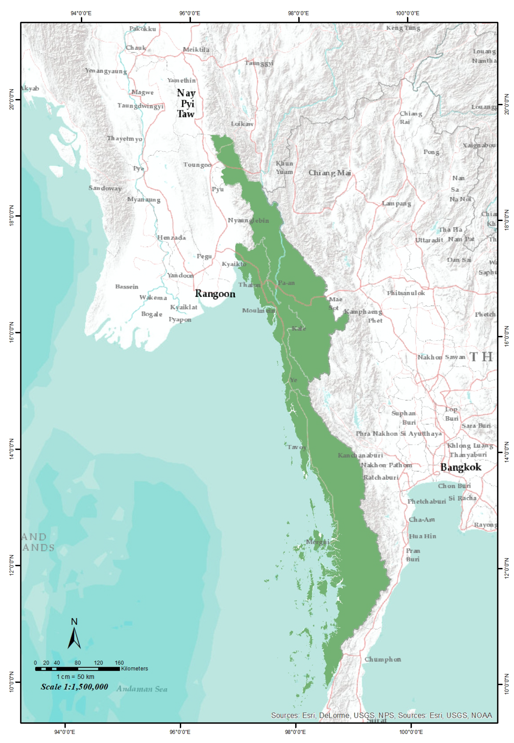
2.1. Study Region
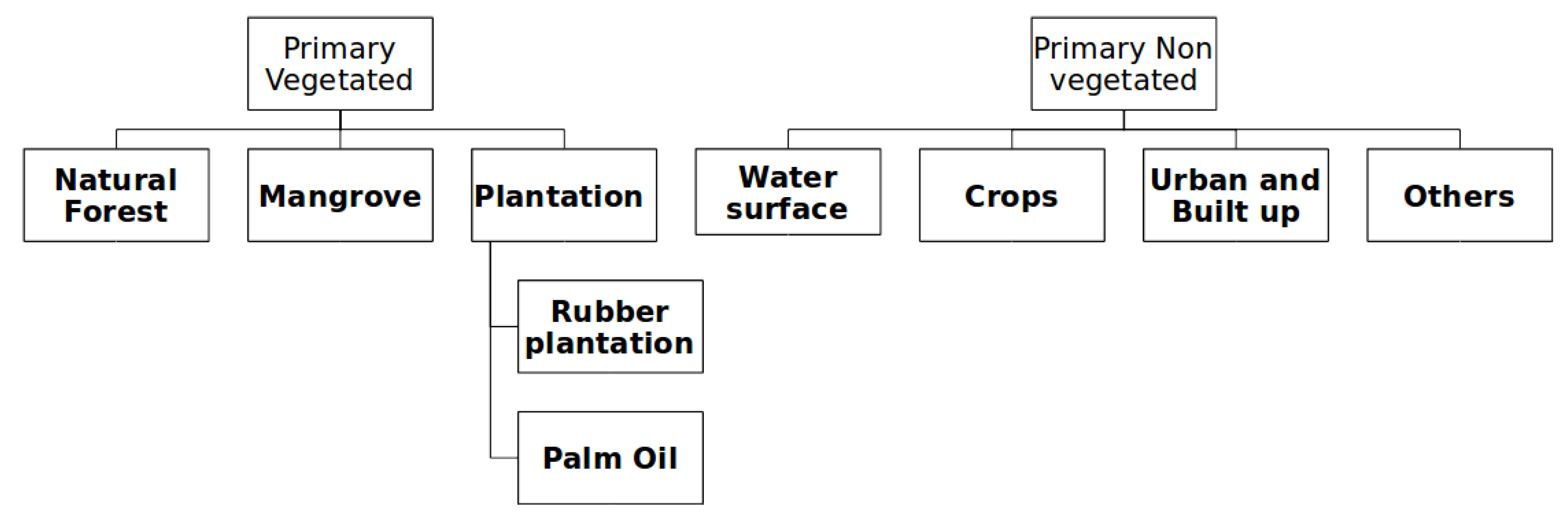
2.2. Typology
- Cropland: land covered by crops and then followed by harvest and a bare soil period [36]. Examples include cereals, oils seeds, rice, vegetables, root crops and forages. This excludes orchards, forest croplands, and forest plantations.
- Forest: Land spanning more than 0.5 hectares with trees higher than 5 m and a canopy cover of more than 10 percent, or trees able to reach these thresholds in situ. It does not include land that is predominantly under agricultural or urban land use [37].
- Mangrove: coastal sediment habitats with more than 10% woody vegetation canopy cover and the majority of cover is higher than 2 m [36].
- Palm oil: The land area designated primarily for production of palm oil. Palm oil grows in tropical climates within 10 degrees of the equator and high rainfall (minimum 1600 mm/year) [38]. Palm oil is a productive crop, it is planted as mono-culture and its expansion comes at the expense of tropical forests [39].
- Rubber plantation: Forest area with rubber tree plantations. Rubber plantation can be inter-crops with other plants, and has about 30–40 years of rotation.
- Surface water: Open water larger than 10 m by 10 m and open to the sky, including fresh and saltwater
- Urban & built up: Cultural lands covered by buildings, roads, and other built structures.
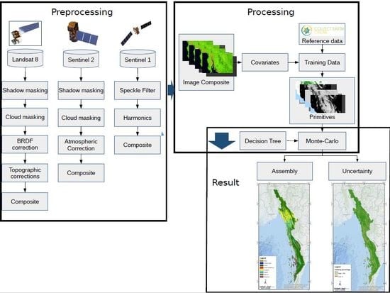
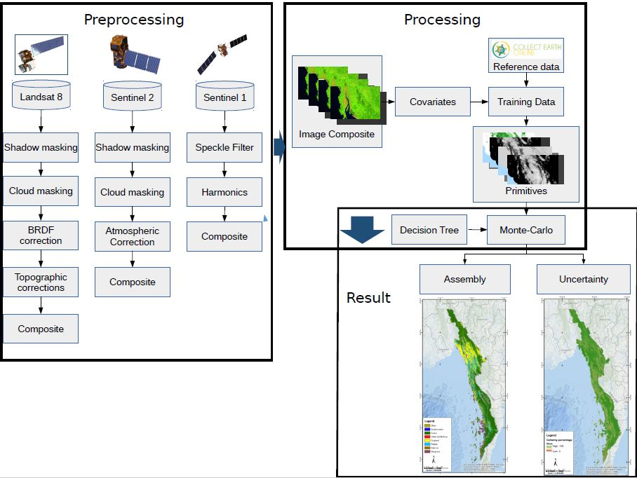
2.3. Methods Overview
2.4. Cloud Shadow Masking
2.5. BRDF Correction
2.6. Topographic Correction
2.7. Representing Vegetation Phenology Using Sentinel-1
2.8. Processing
Covariates
2.9. Reference Data
2.9.1. Training Data
2.9.2. Primitives
2.9.3. Assembly Logic and Monte-Carlo Simulations
2.10. Validation
3. Results
4. Discussion
5. Conclusions
Author Contributions
Funding
Acknowledgments
Conflicts of Interest
Appendix A
References
- Curtis, P.G.; Slay, C.M.; Harris, N.L.; Tyukavina, A.; Hansen, M.C. Classifying drivers of global forest loss. Science 2018, 361, 1108–1111. [Google Scholar]
- Leimgruber, P.; Kelly, D.S.; Steininger, M.K.; Brunner, J.; Müller, T.; Songer, M. Forest cover change patterns in Myanmar (Burma) 1990–2000. Environ. Conserv. 2005, 32, 356–364. [Google Scholar] [CrossRef] [Green Version]
- Bhagwat, T.; Hess, A.; Horning, N.; Khaing, T.; Thein, Z.M.; Aung, K.M.; Aung, K.H.; Phyo, P.; Tun, Y.L.; Oo, A.H.; et al. Losing a jewel—Rapid declines in Myanmar’s intact forests from 2002–2014. PLoS ONE 2017, 12, e0176364. [Google Scholar]
- Connette, G.; Oswald, P.; Songer, M.; Leimgruber, P. Mapping distinct forest types improves overall forest identification based on multi-spectral Landsat imagery for Myanmar’s Tanintharyi Region. Remote Sens. 2016, 8, 882. [Google Scholar]
- LaJeunesse Connette, K.J.; Connette, G.; Bernd, A.; Phyo, P.; Aung, K.H.; Tun, Y.L.; Thein, Z.M.; Horning, N.; Leimgruber, P.; Songer, M. Assessment of mining extent and expansion in Myanmar based on freely-available satellite imagery. Remote Sens. 2016, 8, 912. [Google Scholar]
- Hurni, K.; Fox, J. The expansion of tree-based boom crops in mainland Southeast Asia: 2001 to 2014. J. Land Use Sci. 2018, 13, 198–219. [Google Scholar] [CrossRef]
- Hermosilla, T.; Wulder, M.A.; White, J.C.; Coops, N.C.; Hobart, G.W. Regional detection, characterization, and attribution of annual forest change from 1984 to 2012 using Landsat-derived time-series metrics. Remote Sens. Environ. 2015, 170, 121–132. [Google Scholar] [CrossRef]
- Killmann, W.; Hong, L. Rubberwood-the success of an agricultural by-product. UNASYLVA-FAO 2000, 51, 66–72. [Google Scholar]
- Teoh, Y.P.; Don, M.M.; Ujang, S. Assessment of the properties, utilization, and preservation of rubberwood (Hevea brasiliensis): A case study in Malaysia. J. Wood Sci. 2011, 57, 255–266. [Google Scholar]
- Balsiger, J.; Bahdon, J.; Whiteman, A. The Utilization, Processing and Demand for Rubberwood as a Source of Wood Supply. Asia Pacific Forestry Sector Outlook Study Working Paper Series 50; FAD Regional Office for Asia and the Pacific: Bangkok, Thailand, 2000. [Google Scholar]
- Kenney-Lazar, M.; Wong, G. Challenges and Opportunities for Sustainable Rubber in Myanmar; Center for International Forestry Research (CIFOR): Bogor, Indonesia, 2016. [Google Scholar]
- Li, Z.; Fox, J.M. Rubber tree distribution mapping in northeast Thailand. Int. J. Geosci. 2011, 2, 573. [Google Scholar] [CrossRef]
- Senf, C.; Pflugmacher, D.; Van Der Linden, S.; Hostert, P. Mapping rubber plantations and natural forests in Xishuangbanna (Southwest China) using multi-spectral phenological metrics from MODIS time series. Remote Sens. 2013, 5, 2795–2812. [Google Scholar] [CrossRef]
- Dong, J.; Xiao, X.; Chen, B.; Torbick, N.; Jin, C.; Zhang, G.; Biradar, C. Mapping deciduous rubber plantations through integration of PALSAR and multi-temporal Landsat imagery. Remote Sens. Environ. 2013, 134, 392–402. [Google Scholar]
- Shidiq, I.P.A.; Ismail, M.H.; Kamarudin, N. Initial Results of the Spatial Distribution of Rubber Trees in Peninsular Malaysia Using Remotely Sensed Data for Biomass Estimate; IOP Conference Series: Earth and Environmental Science; IOP Publishing: Bristol, UK, 2014; Volume 18, p. 012135. [Google Scholar]
- Koedsin, W.; Huete, A. Mapping rubber tree stand age using Pléiades Satellite Imagery: A case study in Talang district, Phuket, Thailand. Eng. J. 2015, 19, 45–56. [Google Scholar] [CrossRef]
- Fan, H.; Fu, X.; Zhang, Z.; Wu, Q. Phenology-based vegetation index differencing for mapping of rubber plantations using Landsat OLI data. Remote Sens. 2015, 7, 6041–6058. [Google Scholar]
- Zhai, D.; Dong, J.; Cadisch, G.; Wang, M.; Kou, W.; Xu, J.; Xiao, X.; Abbas, S. Comparison of pixel-and object-based approaches in phenology-based rubber plantation mapping in fragmented landscapes. Remote Sens. 2017, 10, 44. [Google Scholar]
- Razak, J.A.B.A.; Shariff, A.R.B.M.; Ahmad, N.B.; Ibrahim Sameen, M. Mapping rubber trees based on phenological analysis of Landsat time series data-sets. Geocarto Int. 2018, 33, 627–650. [Google Scholar] [CrossRef]
- Xiao, C.; Li, P.; Feng, Z. Monitoring annual dynamics of mature rubber plantations in Xishuangbanna during 1987–2018 using Landsat time series data: A multiple normalization approach. Int. J. Appl. Earth Obs. Geoinf. 2019, 77, 30–41. [Google Scholar] [CrossRef]
- Hurni, K.; Schneider, A.; Heinimann, A.; Nong, D.H.; Fox, J. Mapping the expansion of boom crops in mainland Southeast Asia using dense time stacks of Landsat data. Remote Sens. 2017, 9, 320. [Google Scholar]
- Gutiérrez-Vélez, V.H.; DeFries, R. Annual multi-resolution detection of land cover conversion to oil palm in the Peruvian Amazon. Remote Sens. Environ. 2013, 129, 154–167. [Google Scholar] [CrossRef]
- Kou, W.; Xiao, X.; Dong, J.; Gan, S.; Zhai, D.; Zhang, G.; Qin, Y.; Li, L. Mapping deciduous rubber plantation areas and stand ages with PALSAR and Landsat images. Remote Sens. 2015, 7, 1048–1073. [Google Scholar] [CrossRef]
- Chen, B.; Li, X.; Xiao, X.; Zhao, B.; Dong, J.; Kou, W.; Qin, Y.; Yang, C.; Wu, Z.; Sun, R.; et al. Mapping tropical forests and deciduous rubber plantations in Hainan Island, China by integrating PALSAR 25-m and multi-temporal Landsat images. Int. J. Appl. Earth Obs. Geoinf. 2016, 50, 117–130. [Google Scholar] [CrossRef]
- Roy, D.P.; Lewis, P.; Schaaf, C.; Devadiga, S.; Boschetti, L. The global impact of clouds on the production of MODIS bidirectional reflectance model-based composites for terrestrial monitoring. IEEE Geosci. Remote Sens. Lett. 2006, 3, 452–456. [Google Scholar] [CrossRef]
- Pohl, C.; Van Genderen, J.L. Review article multisensor image fusion in remote sensing: Concepts, methods and applications. Int. J. Remote Sens. 1998, 19, 823–854. [Google Scholar] [CrossRef]
- Chang, N.B.; Bai, K.; Chen, C.F. Integrating multisensor satellite data merging and image reconstruction in support of machine learning for better water quality management. J. Environ. Manag. 2017, 201, 227–240. [Google Scholar] [CrossRef]
- Hilker, T.; Wulder, M.A.; Coops, N.C.; Linke, J.; McDermid, G.; Masek, J.G.; Gao, F.; White, J.C. A new data fusion model for high spatial-and temporal-resolution mapping of forest disturbance based on Landsat and MODIS. Remote Sens. Environ. 2009, 113, 1613–1627. [Google Scholar] [CrossRef]
- Gao, F.; Masek, J.; Schwaller, M.; Hall, F. On the blending of the Landsat and MODIS surface reflectance: Predicting daily Landsat surface reflectance. IEEE Trans. Geosci. Remote Sens. 2006, 44, 2207–2218. [Google Scholar]
- Zhu, X.; Chen, J.; Gao, F.; Chen, X.; Masek, J.G. An enhanced spatial and temporal adaptive reflectance fusion model for complex heterogeneous regions. Remote Sens. Environ. 2010, 114, 2610–2623. [Google Scholar]
- Huang, S.; Crabtree, R.L.; Potter, C.; Gross, P. Estimating the quantity and quality of coarse woody debris in Yellowstone post-fire forest ecosystem from fusion of SAR and optical data. Remote Sens. Environ. 2009, 113, 1926–1938. [Google Scholar] [CrossRef]
- Markert, K.N.; Chishtie, F.; Anderson, E.R.; Saah, D.; Griffin, R.E. On the merging of optical and SAR satellite imagery for surface water mapping applications. Results Phys. 2018, 9, 275–277. [Google Scholar] [CrossRef]
- Bassi, A.M.; Gallagher, L.A.; Helsingen, H. Green economy modelling of ecosystem services along the “Road to Dawei”. Environments 2016, 3, 19. [Google Scholar]
- Gritten, D.; Lewis, S.R.; Breukink, G.; Mo, K.; Thuy, D.T.T.; Delattre, E. Assessing Forest Governance in the Countries of the Greater Mekong Subregion. Forests 2019, 10, 47. [Google Scholar]
- Di Gregorio, A. Land Cover Classification System. Classification Concepts and User Manual, Software version 2; Food and Agriculture Organization of the United Nations: Rome, Italy, 2005. [Google Scholar]
- Loveland, T.R.; Belward, A. The IGBP-DIS global 1km land cover data set, DISCover: First results. Int. J. Remote Sens. 1997, 18, 3289–3295. [Google Scholar] [CrossRef]
- Food and Agriculture Organizations of the United Nations. Global Forest Resources Assessment; Main Report; Food and Agriculture Organizations of the United Nations: Rome, Italy, 2000. [Google Scholar]
- Poku, K. Small-Scale Palm Oil Processing in Africa; Food and Agriculture Organizations of the United Nations: Rome, Italy, 2002; Volume 148. [Google Scholar]
- Teoh, C.H. Key Sustainability Issues in the Palm Oil Sector. A Discussion Paper for Multistakeholders Consultations. Commissioned by the World Bank Group; The World Bank; The International Finance Corporation: Washington, DC, USA, 2010. [Google Scholar]
- Gorelick, N.; Hancher, M.; Dixon, M.; Ilyushchenko, S.; Thau, D.; Moore, R. Google Earth Engine: Planetary-scale geospatial analysis for everyone. Remote Sens. Environ. 2017, 202, 18–27. [Google Scholar]
- Klein, T.; Nilsson, M.; Persson, A.; Håkansson, B. From Open Data to Open Analyses—New Opportunities for Environmental Applications? Environments 2017, 4, 32. [Google Scholar] [Green Version]
- Chen, B.; Xiao, X.; Li, X.; Pan, L.; Doughty, R.; Ma, J.; Dong, J.; Qin, Y.; Zhao, B.; Wu, Z.; et al. A mangrove forest map of China in 2015: Analysis of time series Landsat 7/8 and Sentinel-1A imagery in Google Earth Engine cloud computing platform. ISPRS J. Photogramm. Remote Sens. 2017, 131, 104–120. [Google Scholar] [CrossRef]
- Poortinga, A.; Clinton, N.; Saah, D.; Cutter, P.; Chishtie, F.; Markert, K.N.; Anderson, E.R.; Troy, A.; Fenn, M.; Tran, L.H.; et al. An Operational Before-After-Control-Impact (BACI) Designed Platform for Vegetation Monitoring at Planetary Scale. Remote Sens. 2018, 10, 760. [Google Scholar] [Green Version]
- Markert, K.; Schmidt, C.; Griffin, R.; Flores, A.; Poortinga, A.; Saah, D.; Muench, R.; Clinton, N.; Chishtie, F.; Kityuttachai, K.; et al. Historical and operational monitoring of surface sediments in the lower mekong basin using landsat and google earth engine cloud computing. Remote Sens. 2018, 10, 909. [Google Scholar] [CrossRef]
- Vermote, E.; Justice, C.; Claverie, M.; Franch, B. Preliminary analysis of the performance of the Landsat 8/OLI land surface reflectance product. Remote Sens. Environ. 2016, 185, 46–56. [Google Scholar]
- Holden, C.E.; Woodcock, C.E. An analysis of Landsat 7 and Landsat 8 underflight data and the implications for time series investigations. Remote Sens. Environ. 2016, 185, 16–36. [Google Scholar]
- Roy, D.P.; Kovalskyy, V.; Zhang, H.; Vermote, E.F.; Yan, L.; Kumar, S.; Egorov, A. Characterization of Landsat-7 to Landsat-8 reflective wavelength and normalized difference vegetation index continuity. Remote Sens. Environ. 2016, 185, 57–70. [Google Scholar] [CrossRef] [Green Version]
- Zhu, Z.; Woodcock, C.E. Object-based cloud and cloud shadow detection in Landsat imagery. Remote Sens. Environ. 2012, 118, 83–94. [Google Scholar] [CrossRef]
- Lee, J.S.; Wen, J.H.; Ainsworth, T.L.; Chen, K.S.; Chen, A.J. Improved sigma filter for speckle filtering of SAR imagery. IEEE Trans. Geosci. Remote Sens. 2009, 47, 202–213. [Google Scholar]
- Vermote, E.F.; Tanré, D.; Deuze, J.L.; Herman, M.; Morcette, J.J. Second simulation of the satellite signal in the solar spectrum, 6S: An overview. IEEE Trans. Geosci. Remote Sens. 1997, 35, 675–686. [Google Scholar] [CrossRef]
- Wilson, R.T. Py6S: A Python interface to the 6S radiative transfer model. Comput. Geosci. 2013, 51, 166. [Google Scholar] [CrossRef]
- Zhai, H.; Zhang, H.; Zhang, L.; Li, P. Cloud/shadow detection based on spectral indices for multi/hyperspectral optical remote sensing imagery. ISPRS J. Photogramm. Remote Sens. 2018, 144, 235–253. [Google Scholar] [CrossRef]
- Housman, I.; Chastain, R.; Finco, M. An Evaluation of Forest Health Insect and Disease Survey Data and Satellite-Based Remote Sensing Forest Change Detection Methods: Case Studies in the United States. Remote Sens. 2018, 10, 1184. [Google Scholar]
- Yun, S.I.; Kim, K.S. Sky Luminance Measurements Using CCD Camera and Comparisons with Calculation Models for Predicting Indoor Illuminance. Sustainability 2018, 10, 1556. [Google Scholar] [CrossRef]
- Yang, G.; Li, C.; Wang, Y.; Yuan, H.; Feng, H.; Xu, B.; Yang, X. The DOM generation and precise radiometric calibration of a UAV-mounted miniature snapshot hyperspectral imager. Remote Sens. 2017, 9, 642. [Google Scholar] [CrossRef]
- Wierzbicki, D.; Kedzierski, M.; Fryskowska, A.; Jasinski, J. Quality Assessment of the Bidirectional Reflectance Distribution Function for NIR Imagery Sequences from UAV. Remote Sens. 2018, 10, 1348. [Google Scholar]
- Nicodemus, F.E. Reflectance nomenclature and directional reflectance and emissivity. Appl. Opt. 1970, 9, 1474–1475. [Google Scholar] [CrossRef] [PubMed]
- Roy, D.P.; Ju, J.; Lewis, P.; Schaaf, C.; Gao, F.; Hansen, M.; Lindquist, E. Multi-temporal MODIS–Landsat data fusion for relative radiometric normalization, gap filling, and prediction of Landsat data. Remote Sens. Environ. 2008, 112, 3112–3130. [Google Scholar] [CrossRef]
- Gao, F.; He, T.; Masek, J.G.; Shuai, Y.; Schaaf, C.B.; Wang, Z. Angular effects and correction for medium resolution sensors to support crop monitoring. IEEE J. Sel. Top. Appl. Earth Obs. Remote Sens. 2014, 7, 4480–4489. [Google Scholar] [CrossRef]
- Lucht, W.; Schaaf, C.B.; Strahler, A.H. An algorithm for the retrieval of albedo from space using semiempirical BRDF models. IEEE Trans. Geosci. Remote Sens. 2000, 38, 977–998. [Google Scholar] [CrossRef]
- Colby, J.D. Topographic normalization in rugged terrain. Photogramm. Eng. Remote Sens. 1991, 57, 531–537. [Google Scholar]
- Riaño, D.; Chuvieco, E.; Salas, J.; Aguado, I. Assessment of different topographic corrections in Landsat-TM data for mapping vegetation types (2003). IEEE Trans. Geosci. Remote Sens. 2003, 41, 1056–1061. [Google Scholar]
- Shepherd, J.; Dymond, J. Correcting satellite imagery for the variance of reflectance and illumination with topography. Int. J. Remote Sens. 2003, 24, 3503–3514. [Google Scholar]
- Soenen, S.A.; Peddle, D.R.; Coburn, C.A. SCS+ C: A modified sun-canopy-sensor topographic correction in forested terrain. IEEE Trans. Geosci. Remote Sens. 2005, 43, 2148–2159. [Google Scholar]
- Gu, D.; Gillespie, A. Topographic normalization of Landsat TM images of forest based on subpixel sun–canopy–sensor geometry. Remote Sens. Environ. 1998, 64, 166–175. [Google Scholar] [CrossRef]
- Justice, C.O.; Wharton, S.W.; Holben, B. Application of digital terrain data to quantify and reduce the topographic effect on Landsat data. Int. J. Remote Sens. 1981, 2, 213–230. [Google Scholar] [CrossRef] [Green Version]
- Smith, J.A.; Lin, T.L.; Ranson, K.J. The Lambertian assumption and Landsat data. Photogramm. Eng. Remote Sens. 1980, 46, 1183–1189. [Google Scholar]
- Teillet, P.; Guindon, B.; Goodenough, D. On the slope-aspect correction of multispectral scanner data. Can. J. Remote Sens. 1982, 8, 84–106. [Google Scholar]
- Tadono, T.; Ishida, H.; Oda, F.; Naito, S.; Minakawa, K.; Iwamoto, H. Precise global DEM generation by ALOS PRISM. ISPRS Ann. Photogramm. Remote Sens. Spat. Inf. Sci. 2014, 2, 71. [Google Scholar]
- Takaku, J.; Tadono, T.; Tsutsui, K. Generation of High Resolution Global Dsm From Alos Prism. In Proceedings of the 2014 ISPRS Technical Commission IV Symposium, Suzhou, China, 14–16 May 2014; Volume 2. [Google Scholar]
- Jung, M.; Chang, E. NDVI-based land-cover change detection using harmonic analysis. Int. J. Remote Sens. 2015, 36, 1097–1113. [Google Scholar]
- Shumway, R.H.; Stoffer, D.S. Time series regression and exploratory data analysis. In Time Series Analysis and Its Applications; Springer: Berlin/Heidelberg, Germany, 2011; pp. 47–82. [Google Scholar]
- Shumway, R.H.; Stoffer, D.S. Time Series Analysis and Its Applications (Springer Texts in Statistics); Springer: Berlin/Heidelberg, Germany, 2005. [Google Scholar]
- McFeeters, S.K. The use of the Normalized Difference Water Index (NDWI) in the delineation of open water features. Int. J. Remote Sens. 1996, 17, 1425–1432. [Google Scholar]
- Key, C.H.; Benson, N.C. The Normalized Burn Ratio (NBR): A Landsat TM Radiometric Measure of Burn Severity; United States Geological Survey; Northern Rocky Mountain Science Center: Bozeman, MT, USA, 1999.
- Salomonson, V.V.; Appel, I. Estimating fractional snow cover from MODIS using the normalized difference snow index. Remote Sens. Environ. 2004, 89, 351–360. [Google Scholar]
- Rouse, J., Jr.; Haas, R.; Schell, J.; Deering, D. Monitoring Vegetation Systems in the Great Plains With ERTS. In Proceedings of the Third ERTS Symposium, Washington, DC, USA, 10–14 December 1973; NASA SP-351. pp. 309–317. [Google Scholar]
- Jiang, Z.; Huete, A.R.; Didan, K.; Miura, T. Development of a two-band enhanced vegetation index without a blue band. Remote Sens. Environ. 2008, 112, 3833–3845. [Google Scholar]
- Huete, A.R. A soil-adjusted vegetation index (SAVI). Remote Sens. Environ. 1988, 25, 295–309. [Google Scholar]
- Xu, H. A new index for delineating built-up land features in satellite imagery. Int. J. Remote Sens. 2008, 29, 4269–4276. [Google Scholar]
- R Core Team. R: A Language and Environment for Statistical Computing; R Foundation for Statistical Computing: Vienna, Austria, 2018. [Google Scholar]
- Liaw, A.; Wiener, M. Classification and Regression by randomForest. R News 2002, 2, 18–22. [Google Scholar]
- Breiman, L. Random forests. Mach. Learn. 2001, 45, 5–32. [Google Scholar]
- Saah, D.; Tenneson, K.; Poortinga, A.; Nguyen, Q.; Chishtie, F.; San Aung, K.; Clinton, N.; Anderson, E.R.; Cutter, P.; Goldstein, J.; et al. A novel modular free and open-source system for landcover mapping using cloud-based remote sensing and machine learning. Remote Sens. Environ. 2019. under review. [Google Scholar]
- Binder, K.; Heermann, D.; Roelofs, L.; Mallinckrodt, A.J.; McKay, S. Monte Carlo simulation in statistical physics. Comput. Phys. 1993, 7, 156–157. [Google Scholar] [CrossRef]
- Bey, A.; Sánchez-Paus Díaz, A.; Maniatis, D.; Marchi, G.; Mollicone, D.; Ricci, S.; Bastin, J.F.; Moore, R.; Federici, S.; Rezende, M.; et al. Collect earth: Land use and land cover assessment through augmented visual interpretation. Remote Sens. 2016, 8, 807. [Google Scholar]
- Olofsson, P.; Foody, G.M.; Herold, M.; Stehman, S.V.; Woodcock, C.E.; Wulder, M.A. Good practices for estimating area and assessing accuracy of land change. Remote Sens. Environ. 2014, 148, 42–57. [Google Scholar] [Green Version]
- Pontius, R.G., Jr.; Millones, M. Death to Kappa: Birth of quantity disagreement and allocation disagreement for accuracy assessment. Int. J. Remote Sens. 2011, 32, 4407–4429. [Google Scholar]
- Pontius, R.; Gao, Y.; Giner, N.; Kohyama, T.; Osaki, M.; Hirose, K. Design and interpretation of intensity analysis illustrated by land change in Central Kalimantan, Indonesia. Land 2013, 2, 351–369. [Google Scholar]
- Roy, D.P.; Li, J.; Zhang, H.K.; Yan, L.; Huang, H.; Li, Z. Examination of Sentinel-2A multi-spectral instrument (MSI) reflectance anisotropy and the suitability of a general method to normalize MSI reflectance to nadir BRDF adjusted reflectance. Remote Sens. Environ. 2017, 199, 25–38. [Google Scholar]
- Roy, D.P.; Li, Z.; Zhang, H.K. Adjustment of Sentinel-2 multi-spectral instrument (MSI) Red-Edge band reflectance to Nadir BRDF adjusted reflectance (NBAR) and quantification of red-edge band BRDF effects. Remote Sens. 2017, 9, 1325. [Google Scholar]
- Claverie, M.; Ju, J.; Masek, J.G.; Dungan, J.L.; Vermote, E.F.; Roger, J.C.; Skakun, S.V.; Justice, C. The Harmonized Landsat and Sentinel-2 surface reflectance data set. Remote Sens. Environ. 2018, 219, 145–161. [Google Scholar] [CrossRef]
- Franch, B.; Vermote, E.; Skakun, S.; Roger, J.C.; Santamaria-Artigas, A.; Villaescusa-Nadal, J.L.; Masek, J. Towards Landsat and Sentinel-2 BRDF normalization and albedo estimation: A case study in the Peruvian Amazon forest. Front. Earth Sci. 2018, 6, 185. [Google Scholar]
- Dibs, H.; Idrees, M.O.; Alsalhin, G.B.A. Hierarchical classification approach for mapping rubber tree growth using per-pixel and object-oriented classifiers with SPOT-5 imagery. Egypt. J. Remote Sens. Space Sci. 2017, 20, 21–30. [Google Scholar] [CrossRef]
- Dong, J.; Xiao, X.; Sheldon, S.; Biradar, C.; Xie, G. Mapping tropical forests and rubber plantations in complex landscapes by integrating PALSAR and MODIS imagery. ISPRS J. Photogramm. Remote Sens. 2012, 74, 20–33. [Google Scholar] [CrossRef]
- Chen, G.; Thill, J.C.; Anantsuksomsri, S.; Tontisirin, N.; Tao, R. Stand age estimation of rubber (Hevea brasiliensis) plantations using an integrated pixel-and object-based tree growth model and annual Landsat time series. ISPRS J. Photogramm. Remote Sens. 2018, 144, 94–104. [Google Scholar]
- Kennedy, R.E.; Yang, Z.; Cohen, W.B. Detecting trends in forest disturbance and recovery using yearly Landsat time series: 1. LandTrendr—Temporal segmentation algorithms. Remote Sens. Environ. 2010, 114, 2897–2910. [Google Scholar] [CrossRef]
- Verbesselt, J.; Hyndman, R.; Newnham, G.; Culvenor, D. Detecting trend and seasonal changes in satellite image time series. Remote Sens. Environ. 2010, 114, 106–115. [Google Scholar] [CrossRef]
- Aldwaik, S.Z.; Pontius, R.G., Jr. Intensity analysis to unify measurements of size and stationarity of land changes by interval, category, and transition. Landsc. Urban Plan. 2012, 106, 103–114. [Google Scholar] [CrossRef]
- Torbick, N.; Ledoux, L.; Salas, W.; Zhao, M. Regional mapping of plantation extent using multisensor imagery. Remote Sens. 2016, 8, 236. [Google Scholar]
- Koskinen, J.; Leinonen, U.; Vollrath, A.; Ortmann, A.; Lindquist, E.; d’Annunzio, R.; Pekkarinen, A.; Käyhkö, N. Participatory mapping of forest plantations with Open Foris and Google Earth Engine. ISPRS J. Photogramm. Remote Sens. 2019, 148, 63–74. [Google Scholar]
- Pekel, J.F.; Cottam, A.; Gorelick, N.; Belward, A.S. High-resolution mapping of global surface water and its long-term changes. Nature 2016, 540, 418. [Google Scholar] [PubMed]
- Hansen, M.C.; Potapov, P.V.; Moore, R.; Hancher, M.; Turubanova, S.; Tyukavina, A.; Thau, D.; Stehman, S.; Goetz, S.; Loveland, T.R.; et al. High-resolution global maps of 21st-century forest cover change. Science 2013, 342, 850–853. [Google Scholar]
- Oliphant, A.; Thenkabail, P.; Teluguntla, P.; Xiong, J.; Congalton, R.; Yadav, K.; Massey, R.; Gumma, M.; Smith, C. NASA Making Earth System Data Records for Use in Research Environments (MEaSUREs) Global Food Security-Support Analysis Data (GFSAD) Cropland Extent 2015 Southeast Asia 30 m V001; NASA EOSDIS Land Processes DAAC, USGS Earth Resources Observation and Science (EROS); NASA EOSDIS Land Processes DAAC: Sioux Falls, SD, USA, 2017.
- Chen, Y.; Dou, P.; Yang, X. Improving land use/cover classification with a multiple classifier system using AdaBoost integration technique. Remote Sens. 2017, 9, 1055. [Google Scholar]
- Dube, T.; Mutanga, O.; Elhadi, A.; Ismail, R. Intra-and-inter species biomass prediction in a plantation forest: testing the utility of high spatial resolution spaceborne multispectral rapideye sensor and advanced machine learning algorithms. Sensors 2014, 14, 15348–15370. [Google Scholar]
- Dihkan, M.; Guneroglu, N.; Karsli, F.; Guneroglu, A. Remote sensing of tea plantations using an SVM classifier and pattern-based accuracy assessment technique. Int. J. Remote Sens. 2013, 34, 8549–8565. [Google Scholar]


| Blue | Green | Red | nir | swir1 |
|---|---|---|---|---|
| green | red | swir1 | red | swir2 |
| red | nir | swir2 | swir1 | |
| nir | swir1 | swir2 | ||
| swir1 | swir2 | |||
| swir2 |
| Land Cover Class | No. Training Points |
|---|---|
| Cropland | 1758 |
| Forest | 1422 |
| Mangroves | 873 |
| Palm oil | 1467 |
| Rubber | 1802 |
| Water | 499 |
| Urban and built up | 993 |
| Surface Water | Forest | Urban and Built Up | Cropland | Rubber | Palm Oil | Mangrove | |
|---|---|---|---|---|---|---|---|
| Surface water | 40 | 0 | 6 | 0 | 0 | 0 | 1 |
| Forest | 2 | 1531 | 14 | 18 | 66 | 17 | 0 |
| Urban and Built up | 0 | 0 | 17 | 1 | 0 | 0 | 0 |
| Cropland | 9 | 16 | 2 | 476 | 14 | 6 | 0 |
| Rubber | 4 | 68 | 2 | 84 | 749 | 26 | 0 |
| Palm oil | 2 | 89 | 0 | 2 | 27 | 262 | 1 |
| Mangrove | 11 | 79 | 0 | 22 | 6 | 4 | 163 |
© 2019 by the authors. Licensee MDPI, Basel, Switzerland. This article is an open access article distributed under the terms and conditions of the Creative Commons Attribution (CC BY) license (http://creativecommons.org/licenses/by/4.0/).
Share and Cite
Poortinga, A.; Tenneson, K.; Shapiro, A.; Nquyen, Q.; San Aung, K.; Chishtie, F.; Saah, D. Mapping Plantations in Myanmar by Fusing Landsat-8, Sentinel-2 and Sentinel-1 Data along with Systematic Error Quantification. Remote Sens. 2019, 11, 831. https://doi.org/10.3390/rs11070831
Poortinga A, Tenneson K, Shapiro A, Nquyen Q, San Aung K, Chishtie F, Saah D. Mapping Plantations in Myanmar by Fusing Landsat-8, Sentinel-2 and Sentinel-1 Data along with Systematic Error Quantification. Remote Sensing. 2019; 11(7):831. https://doi.org/10.3390/rs11070831
Chicago/Turabian StylePoortinga, Ate, Karis Tenneson, Aurélie Shapiro, Quyen Nquyen, Khun San Aung, Farrukh Chishtie, and David Saah. 2019. "Mapping Plantations in Myanmar by Fusing Landsat-8, Sentinel-2 and Sentinel-1 Data along with Systematic Error Quantification" Remote Sensing 11, no. 7: 831. https://doi.org/10.3390/rs11070831