Building Extraction from UAV Images Jointly Using 6D-SLIC and Multiscale Siamese Convolutional Networks


1
School of Geomatics, East China University of Technology, Nanchang 330013, China
2
Key Laboratory of Watershed Ecology and Geographical Environment Monitoring, National Administration of Surveying, Mapping and Geoinformation, Nanchang 330013, China
3
Faculty of Geosciences and Environmental Engineering, Southwest Jiaotong University, Chengdu 611756, China
4
School of Water Resources & Environmental Engineering, East China University of Technology, Nanchang 330013, China
*
Author to whom correspondence should be addressed.
Remote Sens. 2019, 11(9), 1040; https://doi.org/10.3390/rs11091040
Submission received: 28 February 2019
/
Revised: 29 April 2019
/
Accepted: 29 April 2019
/
Published: 1 May 2019
(This article belongs to the Special Issue Remote Sensing based Building Extraction)
Abstract
:Automatic building extraction using a single data type, either 2D remotely-sensed images or light detection and ranging 3D point clouds, remains insufficient to accurately delineate building outlines for automatic mapping, despite active research in this area and the significant progress which has been achieved in the past decade. This paper presents an effective approach to extracting buildings from Unmanned Aerial Vehicle (UAV) images through the incorporation of superpixel segmentation and semantic recognition. A framework for building extraction is constructed by jointly using an improved Simple Linear Iterative Clustering (SLIC) algorithm and Multiscale Siamese Convolutional Networks (MSCNs). The SLIC algorithm, improved by additionally imposing a digital surface model for superpixel segmentation, namely 6D-SLIC, is suited for building boundary detection under building and image backgrounds with similar radiometric signatures. The proposed MSCNs, including a feature learning network and a binary decision network, are used to automatically learn a multiscale hierarchical feature representation and detect building objects under various complex backgrounds. In addition, a gamma-transform green leaf index is proposed to truncate vegetation superpixels for further processing to improve the robustness and efficiency of building detection, the Douglas–Peucker algorithm and iterative optimization are used to eliminate jagged details generated from small structures as a result of superpixel segmentation. In the experiments, the UAV datasets, including many buildings in urban and rural areas with irregular shapes and different heights and that are obscured by trees, are collected to evaluate the proposed method. The experimental results based on the qualitative and quantitative measures confirm the effectiveness and high accuracy of the proposed framework relative to the digitized results. The proposed framework performs better than state-of-the-art building extraction methods, given its higher values of recall, precision, and intersection over Union (IoU).
1. Introduction
Building extraction based on remote sensing data is an effective technique to automatically delineate building outlines; it has been widely studied for decades in the fields of photogrammetry and remote sensing, and is extensively used in various applications, including urban planning, cartographic mapping, and land use analysis [1,2]. The significant progress in sensors and operating platforms has enabled us to acquire remote sensing images and 3D point clouds from cameras or Light Detection And Ranging (LiDAR) equipped in various platforms (e.g., satellite, aerial, and Unmanned Aerial Vehicle (UAV) platforms); thus, the methods based on images and point clouds are commonly used to extract buildings [3,4,5].
Building extraction can be broadly divided into three categories according to data source: 2D image-based methods, 3D point cloud-based methods, and 2D and 3D information hybrid methods. 2D image-based building extraction consists of two stages, namely, building segmentation and regularization. Many approaches have been proposed in recent years to extract buildings through very-high-resolution 2D imagery, including the active contour model-based method [6], multidirectional and multiscale morphological index-based method [7], combined binary filtering and region growing method [8], object-based method [9], dense attention network-based method [10], and boundary-regulated network-based method [2]. Although these methods have achieved important advancements, a single cue from 2D images remains insufficient to extract buildings under the complex backgrounds of images (e.g., illumination, shadow, occlusion, geometric deformation, and quality degradation), which cause inevitable obstacles in the identification and delineation of building outlines under different circumstances. Consequently, differentiating building and non-building objects that carry similar radiometric signatures is difficult by using spectral information alone. Existing methods focus more on building qualitative detection than accurate outline extraction, thus requiring further improvement in building contour extraction to satisfy various applications, such as automatic mapping and building change detection.
Unlike 2D remotely-sensed imagery, LiDAR data can provide the 3D information of ground objects, and are especially useful in distinguishing building and non-building objects by height variation. Various approaches based on LiDAR data, such as polyhedral building roof segmentation and reconstruction [11], building roof segmentation using the random sample consensus algorithm [12,13] and global optimization [14], and automatic building extraction using point- and grid-based features [15], have been proposed for building extraction. However, the utilization of height information alone may fail to distinguish building and non-building objects with similar heights, such as houses and surrounding trees with smooth canopies. The accuracy of building extraction often relies on the density of 3D point clouds, and the outline of poor-quality points at the edge of buildings is challenging to accurately delineate. Moreover, most LiDAR-based methods may only be applicable to urban building extraction and may be unsuitable for extracting rural buildings with topographic relief because of the difficulty in giving a certain height threshold to truncate non-building objects. Aside from these limitations, automatic building extraction is challenging in the contexts of complex shape, occlusion, and size. Therefore, automatically extracting buildings by using a single data type, either 2D remotely-sensed images or 3D LiDAR point clouds, remains insufficient.
Many approaches that combine spectral and height information have been proposed to overcome the shortcomings of building extraction using a single data type. In [16,17], Normalized Difference Vegetation Index (NDVI) and 3D LiDAR point clouds were used to eliminate vegetation and generate a building mask, and height and area thresholds were given to exclude other low-height objects and small buildings. A method based on LiDAR point clouds and orthoimage has been proposed to delineate the boundaries of buildings, which are then regulated by using image lines [1]. However, compared with satellite and aerial imagery, LiDAR data are actually difficult to access due to the high cost involved [5]. Tian et al. [18] proposed an approach to building detection based on 2D images and Digital Surface Model (DSM); unlike 3D LiDAR point clouds, height information is generated from stereo imagery by the dense matching algorithm. Moreover, the combination of 2D UAV orthoimages and image-derived 3D point clouds has been used for building extraction on the basis of low-cost and high-flexibility UAV photogrammetry and remote sensing [5,19]. Most civil UAVs only acquire remote sensing images with RGB channels and do not include multispectral bands (e.g., near-infrared bands), that is, eliminating vegetation by the NDVI is not feasible. As an alternative method, RGB-based Multidimensional Feature Vector (MFV) and Support Vector Machine (SVM) classifiers were integrated by Dai et al. [5] to eliminate vegetation; in this method, buildings are extracted by using a certain height threshold (e.g., 2.5 m), and building outlines are regularized by jointly using a line-growing algorithm and a w-k-means clustering algorithm. However, this method is only useful for extracting buildings with linear and perpendicular edges and not applicable to extract buildings with irregular shapes.
On the basis of the advantages of UAV photogrammetry and remote sensing, this study concentrates on building segmentation and outline regularization based on UAV orthoimages and image-derived point clouds. First, image segmentation is implemented to cluster all pixels of UAV orthoimages; SLIC is a popular algorithm for segmenting superpixels and does not require much computational cost [20], but it easily confuses building and image backgrounds with similar radiometric signatures. We accordingly exploit a novel 6D simple linear iterative clustering (6D-SLIC) algorithm for superpixel segmentation by additionally imposing DSM that is generated from image-derived 3D point clouds; DSM helps to distinguish objects from different heights (e.g., building roof and road). Second, the vegetation superpixels are truncated by using a Gamma-transform Green Leaf Index (GGLI). Then, the boundaries of non-vegetation objects are shaped by merging the superpixels with approximately equal heights. Inspired by the progresses made in deep learning in recent years, the deep convolutional neural network is one of the most popular and successful deep networks for image processing because it can work efficiently under various complex backgrounds [21,22,23,24,25,26] and is suitable for identifying building objects under different circumstances. The Fully Convolutional Network (FCN) [27] is a specific type of deep network that is used for image segmentation and building extraction [28]. U-shaped convolutional Networks (U-Nets) are extended for image segmentation [29] and building extraction [30]. In this study, buildings are detected by Multiscale Siamese Convolutional Networks (MSCNs), including a feature learning network and a binary decision network, which are used to automatically learn a multiscale hierarchical feature representation and detect building objects. Finally, the building outlines are regulated by the Douglas–Peucker and iterative optimization algorithms.
The main contribution of this study is to propose a method for building extraction that is suitable for UAV orthoimage and image-derived point clouds. In this method, the improved SLIC algorithm for UAV image segmentation, which helps accurately delineate building boundaries under building and image backgrounds with similar radiometric signatures. MSCNs are used to improve the performance of building detection under various complex backgrounds, and the Douglas–Peucker algorithm and iterative optimization are coupled to eliminate jagged details generated from small structures as a result of superpixel segmentation.
The remainder of this paper is organized as follows. Section 2 describes the details of the proposed method for building extraction. Section 3 presents the comparative experimental results in combination with a detailed analysis and discussion. Section 4 concludes this paper and discusses possible future work.
2. Proposed Method
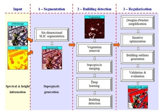
The proposed framework for building extraction consists of three stages, as presented in Figure 1. In the segmentation stage, 6D-SLIC is used to segment superpixels from UAV orthoimages and DSM (generated from image-derived point clouds), and the initial outlines of ground objects are shaped by merging the superpixels. In the building detection stage, a GGLI is used to eliminate vegetation, and the buildings are detected by using the proposed MSCNs (including a feature learning network for deep feature representation and a binary network for building detection). In the regularization stage, the building boundaries are decimated and simplified by removing insignificant vertices using the Douglas–Peucker algorithm. At the same time, the building outlines are regulated by using a proposed iterative optimization algorithm. Finally, the building outlines are validated and evaluated.
2.1. D-SLIC-Based Superpixel Segmentation
Image segmentation is a commonly used and powerful technique for delineating the boundaries of ground objects. It is also a popular topic in the fields of computer vision and remote sensing. The classical segmentation algorithms for remotely-sensed imagery, such as quadtree-based segmentation [31], watershed segmentation [32], and Multi-Resolution Segmentation (MRS) [33], often partition an image into relatively homogeneous regions generally using spectral and spatial information while rarely introducing additional information to assist segmentation (e.g., height information) despite various improved methods for finding solutions to some image datasets [9,34,35,36]. Therefore, the commonly used segmentation methods that are highly dependent on spectral information cannot still break the bottleneck, i.e., sensitivity to illumination, occlusion, quality degradation, and various complex backgrounds. Especially for UAV remote sensing images, a centimeter-level ground resolution provides high-definition details and geometric structural information of ground objects but also generates disturbances, which pose a great challenge in accurately delineating boundaries.
Examples of four types of buildings are given in Figure 2a. The best results of segmentation obtained from classical methods are exhibited in Figure 2b,c; such results are achieved through multiple tests to find the optimal parameters (e.g., scale: 300, shape: 0.4, compactness: 0.8 in MRS). MRS performs better than quadtree-based methods do, but the building boundaries under MRS are still incomplete or confused with backgrounds relative to ground-truth outlines (Figure 2d) because the spectral difference is the insignificant gap at building edges. The accurate outlines of buildings are difficult to delineate from the spectral and spatial information of UAV images. Many strategies can be used to merge the segmented regions to the entities, but finding a generic rule to achieve a perfect solution in a single data source is actually difficult. Most classical algorithms (e.g., MRS) are time and memory consuming when used to segment large remotely-sensed imagery, because they use a pixel grid for the initial object representation [37].
Many deep learning-based algorithms, such as multiscale convolutional network [38], deep convolutional encoder–decoder [39], and FCN [40], have been proposed for the semantic segmentation of natural images or computer vision applications, and prominent progress has been made. However, deep learning-based methods dramatically increase computational time and memory and are thus inefficient for the fast segmentation of large UAV orthoimages. In the current study, a 6D-SLIC algorithm is used to extract initial building outlines by joining height information. SLIC is a state-of-the-art algorithm for segmenting superpixels that does not require much computational resource to achieve effective and efficient segmentation.
In the 6D-SLIC algorithm, superpixels are generated by clustering pixels according to their color similarity and proximity in the 2D image plane space; in this way, the proposed algorithm is similar to the SLIC algorithm [20]. Compared to the five-dimensional (5D) space in the SLIC algorithm, the height information obtained from image-derived 3D point clouds is then used to cluster pixels. Hence, a 6D space is used to generate compact, nearly uniform superpixels, where is defined by the pixel color vector of the CIELAB color space and is the 3D coordinate of a pixel. The pixels in the CIELAB color space are considered perceptually uniform for small color distances, and height information is used to cluster the pixels into the building area with approximately equal heights.
Unlike that in the SLIC algorithm, the desired number of approximately equally sized superpixels is indirectly given in the 6D-SLIC algorithm but is computed on the basis of the minimum area , as follows:
where is the number of pixels in an image and denotes the ground resolution (unit: m). is commonly given as 10 m2 with reference to the minimum area of buildings in The literature [5], whereas 5 m2 is given to consider small buildings in the current study; each superpixel approximately contains pixels, and a superpixel center would exist for roughly equally sized superpixels at every grid interval . superpixel cluster centers with at regular grid intervals are selected. Similar to the SLIC algorithm, the search area of the pixels associated with each cluster is assumed to be within of the 2D image plane space. The Euclidean distance of the CIELAB color space and height are used to define pixel similarity, which is useful in clustering pixels for small distances. The distance measure of the proposed 6D-SLIC algorithm is defined as follows:
where is the sum of the distance , height difference , and the 2D image plane distance normalized by the grid interval ; represents the weight to emphasize the contribution of and , and it is the SLIC distance measure when is set as 1, the weight can be determined by selecting several building samples from the segmented data and performing multiple trials to obtain the optimal superpixel segmentation effect; and is a variable that can be given to control the compactness of a superpixel. The distances of , , and between a pixel () and the cluster center can be computed as follows:
As a result of the high-definition details of UAV images, noisy pixels may be considerable and should be avoided in the selection of a cluster center. A 3D gradient is proposed to control the sampling of cluster centers and move them to the lowest 3D gradient position in a 3×3 neighborhood to avoid placing a cluster center at the edge of buildings. The 3D gradients are computed as
where and denote the gradients of image intensity and height difference, respectively. The two gradients can be computed as
where and represent the vector and height corresponding to the pixel at position , respectively; and denotes the norm. DSM is generated from image-derived 3D point clouds.
All the pixels of the UAV images are associated with the nearest cluster center on the basis of the minimum distance of . The cluster center is then updated by
where is the number of pixels that belong to the cluster center . The new cluster center should be moved to the lowest 3D gradient position again on the basis of the values of Equations (4) and (5). The processes of associating all pixels to the nearest cluster center and recomputing the cluster center are iteratively repeated until the convergence of distance .
After all pixels are clustered into the nearest cluster center, a strategy of enforcing connectivity is employed to remove the small disjoint segments and merge the segments in terms of the approximately equal height in each cluster. Therefore, the initial boundaries of ground objects are shaped by connecting the segments in the vicinity. This definition satisfies the constraint in Equation (7), and clusters and are regarded to belong to the same ground object.
where represents the average operation of height and is a given height threshold, which is set to 2.5 m in this study.
We use an efficient and effective superpixel segmentation on the basis of the SLIC algorithm, which is regarded as a simple and efficient approach that is suitable for large-image segmentation. 3D space coordinates, rather than a 2D image plane space, are selected as a distance measure to cluster all pixels of an image into superpixels. The algorithm is expressed below, and the comparisons of superpixel segmentation based on the SLIC and 6D-SLIC algorithms are shown in Figure 3. The building areas are identified by vegetation removal and Siamese-typed networks (described in Section 2.2 and Section 2.3), except for the regions merging on the basis of height similarity.
| Algorithm 1: 6D-SLIC segmentation |
| Input: 2D image and . Parameters: minimum area , ground resolution , compactness , weight , maximum number of iterations , number of iterations , minimum distance . Compute approximately equally sized superpixels . Compute every grid interval . Initialize each cluster center . Perturb each cluster center in a 3×3 neighborhood to the lowest 3D gradient position. repeat for each cluster center do Assign the pixels to based on a new distance measure (Equation (2)). end for Update all cluster centers based on Equations (5) and (6). Compute residual error between the previous centers and recomputed centers . Compute . until or Enforcing connectivity. |
Figure 3 depicts that the boundaries of the superpixels at the building edges obtained from the proposed 6D-SLIC algorithm are closer to the true boundaries of buildings than those obtained from the SLIC algorithm are. Additionally, other four state-of-the-art methods (e.g., Entropy Rate Superpixels (ERS) [41], Superpixels Extracted via Energy-Driven Sampling (SEEDS) [42], preemptive SLIC (preSLIC) [43], and Linear Spectral Clustering (LSC) [44]) are used to compare with the 6D-SLIC algorithm, as shown in Figure 4, the four methods do not perform better, and the 6D-SLIC algorithm also shows more similar shapes to the ground-truth maps of the buildings. Moreover, the metrics, e.g., standard boundary recall and under-segmentation error [45], are used to measure the quality of boundaries between building over-segments and the ground-truth. From the visual assessment and the statistical results of two quantitative metrics in Table 1, it can be inferred that the 6D-SLIC algorithm performs better than the SLIC algorithm and other four state-of-the-art methods do due to the additional height information used for superpixel segmentation in the 3D space instead of a 2D image plane space.
2.2. Vegetation Removal
In this study, height similarity is not immediately used to merge superpixels for generating initial building boundaries after 6D-SLIC segmentation because the vegetation surrounding buildings with similar heights may be classified as part of these buildings. An example is given in Figure 5. The image-derived 3D point clouds show that the tree canopies have approximately equal heights relative to the nearby buildings; therefore, the surrounding 3D vegetation points are the obstacle and noise for building detection. Vegetation removal is used to truncate vegetation superpixels for further processing to improve the robustness and efficiency of building detection.
The NDVI is commonly used to detect vegetation on the basis of near-infrared information, but it is unavailable to 3D image-derived point clouds with true color (RGB) in most UAV remotely-sensed imagery. Thus, many vegetation indices based on the RGB system are proposed, and they include the normalized green–red difference index (NGRDI) [46], visible atmospherically resistant index (VARI) [47], green leaf index (GLI) [48], ratio index (RI) [49], and excess green minus excess red (ExG–ExR) [50]. Figure 4d–h show the extracted vegetation information of Figure 5a using the five vegetation indices. GLI performs better than NGRDI, VARI, GLI, and ExG–ExR do. A suitable intensity threshold is actually difficult to set to separate vegetation from the results of the vegetation index calculation. In [5], a standard SVM classification and a priori training data were employed to extract vegetation from an MFV, which was integrated by the five vegetation indices. However, the method may not achieve a satisfying result when a priori training data are not representative, and the poor vegetation indices also reduce the performance of vegetation extraction. Therefore, in this study, a GGLI is created to extract vegetation by enhancing vegetation intensity and using a self-adaptive threshold. The GGLI is defined as follows:
where denotes the gamma value, which is set to 2.5 that is approximately estimated based on the range of 0 to 255 of GGLI value in this study; and , , are the three components of RGB color. Figure 5i shows that the proposed GGLI performs better than the other five vegetation indices do. When the number of pixels belonging to vegetation in the superpixel is more than half of the number of pixels in the superpixel , then the superpixel is considered a vegetation region. The definition satisfies the constraint in Equation (9), and the superpixel is classified into a vegetation region.
where denotes the calculation operator of the number of pixels, denotes the pixel belonging to vegetation , and is the region of the superpixel . The value of a pixel is more than 0.5 times the maximum value in the entire image, and the pixel is classified into vegetation. Tests using UAV data, including two urban and two rural areas with different vegetation covers, are conducted. Figure 6 shows the receiver operating characteristics (ROCs) of the five popular indices and the proposed GGLI. The true positive rate and false positive rate of vegetation are computed on the basis of the number of true positives (), true negatives (), false positives (), and false negatives (). Over 92.3% of vegetation can be correctly extracted by the proposed GGLI, and the FPs are mainly caused by roads and bare land. Hence, the proposed GGLI achieves the best performance in vegetation detection among all vegetation indices. The vegetation superpixels can be effectively detected and removed with the proposed GGLI, and non-vegetation ground objects are shaped by merging the superpixels on the basis of height similarity.
2.3. Building Detection Using MSCNs
After the removal of vegetation superpixels, there still exist some non-building superpixels that are meaningless for further delineation of building outlines and should thus be eliminated. Building detection is commonly achieved by classification or recognition of ground objects, in which many types of features, such as color, texture, and geometric structure, are used to directly or indirectly represent building characteristics by feature descriptors. However, most manually designed features remain insufficient to extract buildings from UAV images with high-definition details under various complex backgrounds (e.g., shadow, occlusion, and geometric deformation).
In this paper, we present MSCNs used in building recognition as feature representation using a convolutional network can work efficiently under various complex backgrounds. We aim to learn deep convolutional networks that can discriminate building and non-building ground objects by 2D UAV image and height information. In our case, the discriminative training of buildings does not rely on labels of individual ground objects but on pairs of 2D UAV images and their height information. Multiscale Siamese-typed architecture is suitable for achieving this goal due to three reasons. First, MSCNs are capable of learning generic deep features, which are useful for making predictions on unknown non-building class distributions even when few examples are available in these new distributions. Second, MSCNs are easily trained using a standard optimization technique on the basis of pairs sampled from 2D images and 3D height information. Third, the sizes of buildings in UAV images vary from small neighborhoods to large regions containing hundreds of thousands of pixels. The feature maps displayed in Figure 7 indicate that the small local structures of buildings tend to respond to small convolutional filters, whereas the coarse structures tend to be extracted by large filters. Thus, multiscale convolutional architecture is suitable to extract the detailed and coarse structures of buildings.
The architecture of the proposed MSCNs is shown in Figure 8, and it includes input, feature learning networks, binary decision networks, and output. In this study, input patches are extracted from the merged superpixels. The feature learning network consists of two streams of convolutional and max-pooling layers, three convolutional layers are arranged for feature extraction in each stream, and two max-pooling layers are inserted in between successive convolutional layers to reduce the number of parameters and the computation in MSCNs. Batch normalization [51] is also inserted into each convolutional layer before the activation of neurons. Three subconvolutional layers arranged for the convolutional layers of Conv_x1, Conv_x2, Conv1, and Conv2 are to extract the feature from multiscale space. The convolutional layers Conv1 and Conv2 in two streams share identical weights, whereas Conv_x1 and Conv_x2 do not because of the different inputs of and . The binary decision network consists of two fully connected layers, and the outputs of MSCNs are predicted as 1 and 0 corresponding to building and non-building regions, respectively.
In the proposed MSCNs, the output of the th hidden vector in the th layer via the operators of linear transformation and activation can be expressed as
where is the th hidden vector in the th layer; is the number of hidden vectors in the th layer; and represent the weights (or convolution kernels with size in the convolutional layers) and biases, respectively; is the dot product (or convolution operator in the convolutional layers); and denotes the activation function. ReLU is applied to the feature learning and binary decision networks, and sigmoid is used in the output of MSCNs. In this study, discriminative training is prone to achieve the binary output of building and non-building probabilities, which are restricted between 0 and 1. Hence, sigmoid function (), instead of ReLU, is used to compute the building and non-building probabilities of a ground object, and the global cost function is an alternative function of the hinge-based loss function with regard to sigmoid output. The proposed MSCNs are trained in a supervised manner by minimizing the global cost function .
where denotes the predicted results of the output layer; refers to the expected output values (i.e., 0 and 1 in this study) given in a supervised manner; and are the numbers of trained data and layers, respectively; is a weight decay parameter; and and are the numbers of hidden vectors in layers and , respectively. The optimization of the proposed MSCNs is achieved by using the standard back-propagation algorithm based on stochastic gradient descent. The update rule of weights and biases at epoch can be written as
where is the learning rate and is momentum. We let , and the partial derivatives with respect to the weight and bias between the layer and the successive layer can be computed by
The residual errors and of the output layer and back propagation in the th feature map of the th convolutional layer can be computed as
In this study, the two outputs of MSCNs are considered building probability and non-building probability , which are used to define whether a non-vegetation object belongs to a building. The two probabilities satisfy the constraint in Equation (18), and the non-vegetation object is regarded as a building region.
where and are two given thresholds.
2.4. Building Outline Regularization
Once a building and its initial outline have been determined, the next step is to refine the building outline. An initial outline of a building is shown in Figure 9a. Many points are located in the same line segment, and the building edges are jagged and disturbed by small structures because of pixel-wise segmentation. The initial outline should be optimized by eliminating low-quality vertices and regularizing line segments. For this task, an iterative optimization algorithm, which utilizes the collinear constraint, is applied to regulate the building boundary. This algorithm consists of the following steps:
(1) The Douglas–Peucker algorithm [52,53] is used to optimize building outlines by simplifying the curves that are approximated by a few vertices; the simplified outline is shown in Figure 9b.
(2) The consecutive collinear vertex , which satisfies the condition that the angle (as shown in Figure 9c) between two adjacent line segments , is determined. Vertex is added to a candidate point set to be eliminated.
(3) Step (2) is repeated by tracking the line segments sequentially from the first vertex to the last vertex until all vertex set of the outline is traversed. The vertices of initial outline belonging to the point sets are eliminated from the vertex set , the vertex set is updated, and the candidate point set is set as null.
(4) Steps (2) and (3) are repeated until no more consecutive collinear vertex is added to the candidate point set .
(5) The vertex set is tracked sequentially from the first vertex to the last vertex; two adjacent vertices and are considered too close if they satisfy the condition that the distance (as shown in Figure 9c) between and is less than a given threshold (0.5 m). One of and is eliminated, and the vertex set is updated.
(6) Step (5) is repeated until no more vertex needs to be eliminated, and the outline is reconstructed by the vertex set .
Figure 9d shows that the proposed iterative optimization algorithm can effectively reduce the superfluous vertices while reconstructing a relatively regular building shape.
3. Experimental Evaluation and Discussion
3.1. Data Description
Two datasets for building extraction are collected by a UAV aerial photogrammetry system, which comprises a UAV platform, one digital camera, a global positioning system, and an inertial measurement unit, to evaluate the performance of the proposed method. The digital camera selected to capture low-altitude UAV remotely-sensed imagery is a SONY ILCE-7RM2 35 mm camera. The test datasets were captured over Zunqiao of Jiangxi Province of China (N, E) in the summer of 2016, during which the UAV flew upward for approximately 400 m. These study areas include urban and rural areas, which are characterized by different scales, different roofs, dense residential, tree surrounding, and irregular shape buildings. Structure from motion [54] and bundle adjustment are used to yield high-precision relative orientation parameters of all UAV remotely-sensed images and recover 3D structures from 2D UAV images, which are referenced by using ground control points collected from high-precision GPS/RTK equipment. Dense and precise 3D point clouds with an approximately average point spacing of 0.1 m are derived from corresponding UAV images using a multiview matching method [55] and can thus provide a detailed 3D structure description for buildings. These image-derived 3D point clouds are also used to generate high-resolution UAV orthoimages and DSMs. Two subregions of Zunqiao are selected for building extraction with two datasets of 3501 × 3511 and 1651 × 3511 pixels. The experimental datasets are shown in Figure 10. The two selected regions include not only urban and rural buildings of different materials, different spacings, different colors and textures, different heights, and complex roof structures, but also, complex backgrounds (e.g., topographic relief, trees surrounding buildings, shadow next to buildings, and roads that resemble building roofs).
To facilitate the comparison, the proposed method was also evaluated on an open benchmark dataset, the International Society for Photogrammetry and Remote Sensing (ISPRS) 2D semantic labeling contest (Potsdam), which can be downloaded from the ISPRS official website (http://www2.isprs.org/commissions/comm3/wg4/2d-sem-label-potsdam.html). The dataset contains 38 patches (of the same size, i.e., 6000 × 6000 pixels), each consisting of a very high-resolution true orthophoto (TOP) tile that is extracted from a larger TOP mosaic, and the corresponding DSMs were also provided. The ground sampling distance of both, the TOP and the DSM, is 5 cm. And the buildings were labeled in the ground truth. In this study, to be as consistent as possible with the UAV images, and to evaluate the performance of distinguishing building roof from ground, two very high-resolution true orthophoto tiles that are partially similar in texture and spectral characteristics (e.g., cement road and bare land), are selected to evaluate the proposed method, as shown in Figure 11.
We provide the referenced building outlines, namely, ground-truth building outlines, that are extracted by manually digitizing all recognizable building outlines using ArcGIS software to verify the accuracy of the proposed method and compare it with other state-of-the-art methods. The boundary of each building is difficult to manually interpret by UAV orthoimage alone; therefore, we digitize the boundaries of buildings by the combination of UAV orthoimage and DSM. The two datasets contain 99 and 34 buildings separately. Figure 10a shows many buildings with boundaries that are not rectilinear and not mutually perpendicular or parallel. The ground-truth buildings of the four experimental datasets are given in Figure 12, some buildings with boundaries that are not rectilinear and not mutually perpendicular or parallel are shown in Figure 12a,c,d.
3.2. Evaluation Criteria of Building Extraction Performance
The results of building extraction using the proposed method and other existing methods are evaluated by overlapping with them with the ground-truth maps on the basis of previous reference maps of buildings. Four indicators are used to evaluate the classification performance of buildings and non-buildings: (1) the number of building regions correctly classified as belonging to buildings (i.e., TP), (2) the number of non-building regions incorrectly classified as belonging to buildings (i.e., FP), (3) the number of non-building regions correctly classified as belonging to non-buildings (i.e., TN), and (4) the number of building regions incorrectly classified as belonging to non-buildings (i.e., FN). Three metrics (i.e., completeness, correctness, and quality) are used to assess the results of building detection, which are computed as [56]
where (i.e., completeness) is the proportion of all actual buildings that are correctly identified as buildings, (i.e., correctness) is the proportion of the identified buildings that are actual buildings, and (i.e., quality) is the proportion of the correctly identified buildings in all actual and identified buildings. The identified building or non-building regions are impossible to completely overlap with the corresponding regions in the reference maps. Therefore, we define two rules to judge whether a region is correctly identified to the corresponding category. First, the identified region that overlaps the reference map belongs to the same category. Second, the percentage of the area of the identified region that overlaps the reference map is more than 60% [9].
Although , , and are the popular metrics to assess the results of building detection, these metrics remain insufficient to measure how good the overlap is between an outline of a building and the corresponding outline in the reference map. Hence, we use three other metrics, i.e., Recall, Precision, and intersection over Union (IoU) [57], to quantitatively evaluate the delineation performance of building outline. As shown in Figure 13, and are respectively the ground truth and the extracted building area, then , , and can be computed as
3.3. MSCNs Training
The training datasets of MSCNs are generated from UAV orthoimages and DSMs, which are obtained by photogrammetric techniques. The datasets include buildings of multiscale, different colors and heights, and complex roof structures in urban and rural areas. The datasets also contain patches with complex backgrounds, such as shadows, topographic relief, and trees surrounding buildings. A total of 50,000 pairs of patches (half building and half non-building patches) with a fixed size of 127 × 127 pixels are extracted in a supervised manner from the UAV orthoimages and DSMs that do not include the experimental images. The non-building patch examples are generated by two ways. First, we randomly select patches from non-building areas, which are determined by manually masking building areas. Second, some examples that are easily confused with buildings are specially selected from the regions of roads, viaducts, and railways to supplement non-building patches. Furthermore, 150,000 pairs of patches are extended to avoid overfitting by image rotation (e.g., 90°, 180°, and 270°), Gaussian blur, and affine transformation. Therefore, the total number of patch pairs is 200,000, in which 195,000 and 5,000 pairs of patches are randomly selected as training and test datasets, respectively.
At the training stage of MSCNs, a batch size of 100 is used as the input; hence, 1950 iterations exist in each epoch. The MSCNs are trained in parallel on NVIDIA GPUs, and training is forced to terminate when the average value of the loss function is less than 0.001 or the epochs are more than 100. The weights of convolutional and fully connected layers are initialized by random Gaussian distributions [58]. The momentum and weight decay are fixed at 0.9 and 0.0005, respectively. The initial learning rate is set to 0.01 and then gradually reduced by using a piecewise function [25] to accelerate the training of MSCNs. Another metric, namely, overall accuracy (), is used to evaluate the performance of building and non-building classification for quantitatively assessing the training performance of the proposed MSCNs. is computed as
in which , , , and are defined in Section 3.2.
We train three Siamese networks, namely, SCNs3, SCNs5, and SCNs7, to evaluate the effects of Siamese networks with and without multiscale. Here, a convolution operator is achieved by using one of the filters with sizes of 3 × 3, 5 × 5, and 7 × 7 in our model. We also evaluate the effect of layer number in our model by adding one convolutional layer to train and test the datasets, namely, MSCNs(layer+). The trained model achieves state-of-the-art results in training and test datasets (Table 2), and Figure 14 shows the changes in and the losses with increasing epochs during the training of MSCNs. Our network and the deeper network (layer+) achieve higher accuracies than SCNs3, SCNs5, and SCNs7 do. Although the deeper network (layer+) performs slightly better than MSCNs do, the convergence of MSCNs(layer+) is slower than that of MSCNs. MSCNs(layer+) converge at nearly 24 epochs ( iterations), whereas MSCNs converge at nearly 30 epochs ( iterations). In addition, MSCNs perform better than SCNs3, SCNs5, and SCNs7 do in terms of , , and . The experimental results demonstrate the effective performance of MSCNs given the tradeoff between accuracy and network complexity.
3.4. Comparisons of MSCNs and Random Forest Classifier
After vegetation removal and superpixel merging, many non-building regions remain. Postprocessing is needed to further classify building and non-building regions. The identified vegetation and the remaining regions after vegetation removal are shown in Figure 15. A classifier of MSCNs is designed for building detection in this study due to its capability of non-linear estimation and the robustness of object classification under complex backgrounds. Another classifier, named Random Forest, has been proven to perform efficiently in the classification of building and non-building regions in the literature [59], in which an experiment comparing Random Forest with MSCNs was conducted to test the effectiveness of the MSCN classifier. Multiple features were extracted to classify using Random Forest and compared to deep features. Table 3 provides the details of multiple features and the parameters of the Random Forest classifier. The experimental results of the ISPRS dataset are given in Figure 16, Figure 17 shows the confusion matrices of building and non-building classification obtained from the Random Forest classifier and MSCNs in the four experimental datasets.
Figure 17 shows that the performance of the proposed MSCNs is better than that of the Random Forest classifier that uses the color histogram, bag of SIFT, and Hog in terms of confusion matrices. Almost all buildings in the two experimental datasets are correctly identified by using the proposed MSCNs, whereas the building identification accuracy of the Random Forest classifier based on color histogram and the bag of SIFT is less than 85%, and that based on Hog is less than 90%. This finding is attributed to two reasons. First, height is combined with spectral information for jointly distinguishing building and non-building ground objects. This approach helps determine a clear gap between building and other ground objects that are similar in texture and spectral characteristics (e.g., cement road and bare land). Second, deep learning-based networks can extract non-linear and high-level semantic features that are not easily affected by image grayscale variations, and they show higher robustness than the other three low-level manually designed features (color histogram, bag of SIFT, and Hog) do. Figure 18 shows the feature representation of the color histogram, bag of SIFT, Hog, and MSCNs. The influence of grayscale variations is given by simulation. Hog is more robust to gray variations than color histogram and SIFT are, the feature vectors extracted by color histogram are easily affected by image grayscale variations, and the feature vectors extracted by SIFT in the dimension of 0 to 20 are different. Compared with the visualization of the three low-level manually designed features, as shown in Figure 18i, that of high-level deep features obtained by the proposed MSCNs shows high similarity to Figure 18a,e under grayscale variations. This result proves that the proposed MSCNs perform with high stability for feature extraction.
3.5. Comparisons of Building Extraction Using Different Parameters
In the 6D-SLIC-based algorithm, the initial size and compactness of superpixels and the weight of height are the three key parameters that affect the extraction of building boundaries. The metric (i.e., ) are used to evaluate the effects of building extraction. Figure 19 shows the results of segmentation with different initial sizes of superpixels (e.g., 3, 5, 10, and 15 m2; i.e., 17 × 17, 22 × 22, 31 × 31, and 38 × 38 pixels inferred by Equation (1)), different compactness values (e.g., 10, 20, 30, and 40), and different weights (e.g., 0.2,0.4, 0.6, and 0.8).
Figure 19a depicts that 6D-SLIC at 5 m2 initial size of superpixels performs better than it does at other sizes in terms of . The superpixel merging of the small size (e.g., 3 m2) is susceptible to UAV image-derived poor-quality 3D point clouds at the edge of buildings (as shown in Figure 3 and Figure 4) that result in the shrinkage of building boundaries. By contrast, the superpixel merging of the larger size (e.g., 10 and 15 m2) may be insensitive to building boundary identification because building details are ignored. Therefore, the results of 6D-SLIC at 3, 10, and 15 m2 initial sizes are worse than those at 5 m2 initial size. Figure 19b shows a trade-off between spatial proximity and pixel similarity of color and height information when the compactness value is set to 20. A good segmentation performance can be achieved when the weight is set as 0.6 in Figure 19c, which is also a trade-off of the contribution between distance and height difference .
3.6. Comparisons of the Proposed Method and State-of-the-Art Methods
Our work uses the proposed 6D-SLIC algorithm as the building outline extractor in the image segmentation part as it allows the full use of the spectral and terrain information of UAV remotely-sensed imagery. The proposed MSCNs with nine layers are then used to classify building and non-building areas. The state-of-the-art results have fewer parameters and involve less computation than the results of two of the most popular networks for image segmentation, i.e., FCN [27] and U-Net [29], do.
To testify the superpixel segmentation performance of the proposed 6D-SLIC algorithm for building extraction, ERS, SEEDS, preSLIC, and LSC are used to extract building from the four experimental datasets. For a fair comparison, the segmented subregions are merged on the basis of the height similarity in the neighborhoods, and the optimal segmentations of ERS, SEEDS, preSLIC, and LSC are achieved through many repeated trials. Also, we select three other state-of-the-art methods, namely, UAV data- (i.e., see Dai [5]), FCN-, and U-Net-based methods, for comparison and analysis to evaluate the proposed building extraction method. The open-source code and pretrained weights of FCN and U-Net are respectively collected from the corresponding GitHub to ensure the repeatability of the experiments. The training samples generated from the UAV images are used for the parameter fine tuning of FCN and U-Net.
Table 4 and Table 5 present the comparative results of , , and values using the six superpixel segmentation algorithms (i.e., SLIC, ERS, SEEDS, preSLIC, LSC, and 6D-SLIC) before and after the regularization. 6D-SLIC achieves a better performance than the other five algorithms do in terms of the , , and values. The building outlines obtained from 6D-SLIC are closest to the ground-truth maps, whereas the regions at the building edges with similar colors are easily confused in the other five algorithms and result in poor building extraction. From the comparison of before and after the regularization, it can be inferred that the proposed regularization can also improve the performance of building extraction that uses the six superpixel segmentation algorithms.
The experimental results of Dai’s method, FCN, U-Net are also given in Table 6. A certain height threshold (e.g., 2.5 m is used in the method of Dai [5]) is difficult to give for separating building points; thus, some low-height buildings shown in the results of Dai in Figure 20a,e are incorrectly identified, resulting in a smaller value than that achieved by the other three methods. The FCN- and U-Net-based methods, which allow deep neural network-based semantic segmentation that is robust and steady for pixel-wise image classification, work efficiently for building detection, and almost all buildings can be identified, as shown in Table 6 and Figure 20. However, the FCN-based method is sensitive to noise, and it cannot accurately extract the building outlines in some regions, such as the shadows shown in the result of FCN in Figure 20b. In comparison with the FCN-based method, the U-Net-based method performs better in single-house-level building outline extraction, as shown in Figure 20. Overall, our method demonstrates superior performance in terms of major metrics and building outline delineation.
In addition, it can be inferred that the computational cost of our method is much less than FCN- and U-Net-based methods because their architectures include more complex convolutional operations with a high computational cost. During our computational efficiency analysis, our method also shows a significant improvement in computational cost in terms of testing (less than one-fifth of the time consumed by the FCN- and U-Net-based methods operated in parallel on NVIDIA GPUs).
The experimental results indicate that the proposed framework presents more significant improvements than the other methods do in terms of the effectiveness and efficiency of building extraction, which can be explained by a number of reasons. First, the point clouds provide valuable information for building extraction, the 6D-SLIC algorithm can rapidly cluster pixels into superpixels by utilizing UAV image spectral information and image-derived point clouds; the latter helps accurately delineate the outline of ground objects despite the existence of similar intensity and texture at building edges in Figure 3. Second, the proposed GGLI can significantly remove vegetation and improve the efficiency of building detection. Third, the deep and salient features learned by a Siamese-type network are more useful and stable in classifying building and non-building areas, even in this case of image intensity dramatic variations, in comparison with the manually designed features in Figure 18. Finally, the proposed building outline regularization algorithm integrates the Douglas–Peucker and iterative optimization algorithms that can remove superfluous vertices and small structures, i.e., the pruned processing is useful to improve the precision of building delineation.
In the method of Dai, the height of the off-terrain points is calculated by a certain threshold that is unstable; thus, some buildings that are not in this threshold are incorrectly identified. The assumption that only the geometry of two mutually perpendicular directions exists in buildings, i.e., the building boundary regularization has limitations for accurately delineating non-regular buildings, is referred to. In the FCN-based method, the subsampling and upsampling operations may cause the information loss of input images, and thus, the prediction results of buildings often have blurred and inaccurate boundaries of buildings, as shown in the results of FCN in Figure 20. In the U-Net-based method, despite the skip connections added to achieve superior performance in comparison with the FCN-based method, pixel-wise classification solely relies on the features within a localized receptive field; therefore, it is still insufficient to capture the global shape information of building polygons, and it is sensitive to noisy data. That is, the architectures of FCN and U-Net are not perfect enough, and there are restrictions on performance improvement. As a result, small structures may exist in building boundaries. The experimental results imply that the low-level manually designed features are unsuitable for building detection because of the influences of grayscale variations. FCN- and U-Net-based methods are difficult to use in extracting the regulated boundaries of buildings when noisy data are present. Our method performs better not only because the point clouds provide valuable information but also is much less computational cost in comparison with FCN- and U-Net-based methods.
4. Conclusions
In this paper, we present a framework to effectively extract building outlines by utilizing a UAV image and its image-derived point clouds. First, a 6D-SLIC algorithm is introduced to improve superpixel generation performance by considering the height information of pixels. Initial ground object outlines are delineated by merging superpixels with approximately equal height. Second, GGLI is used to eliminate vegetation for accelerating building candidate detection. Third, MSCNs are designed to directly learn deep features and building confirmation. Finally, the building boundaries are regulated by jointly using the Douglas–Peucker and iterative optimization algorithms. The statistical and visualization results indicate that our framework can work efficiently for building detection and boundary extraction. The framework also shows higher accuracy for all experimental datasets according to qualitative comparisons performed with some state-of-the-art methods for building segmentation, such as UAV data-based method and two semantic segmentation methods (e.g., FCN- and U-Net-based methods). The results prove the high capability of the proposed framework in building extraction from UAV data.
The proposed building extraction framework highly relies on the quality of photogrammetric processing. UAV image-derived poor-quality point clouds at building edges can decrease the accuracy of building boundary extraction. In addition, there are many parameters used in the proposed method, these parameters are referred from literature or determined based on the best trials.
In future studies, we will optimize our framework to achieve the best performance through a collinear constraint and by reducing the dependence on the quality of image-derived point clouds. We will also try to improve the proposed method by reducing the related parameters, and improve the architecture of U-Net to suit for building extraction from RGB bands and the point clouds for further comparing with the proposed method.
Author Contributions
H.H. proposed the framework of extracting buildings and wrote the source code and the paper. J.Z. and M.C. designed the experiments and revised the paper. T.C. and P.C. generated the datasets and performed the experiments. D.L. analyzed the data and improved the manuscript.
Funding
This study was financially supported by the National Natural Science Foundation of China (41861062, 41401526, and 41861052) and Natural Science Foundation of Jiangxi Province of China (20171BAB213025 and 20181BAB203022).
Acknowledgments
The authors thank Puyang An providing datasets. The authors also thank the editor-in-chief, the anonymous associate editor, and the reviewers for their systematic review and valuable comments.
Conflicts of Interest
The authors declare no conflict of interest.
References
- Gilani, S.A.N.; Awrangjeb, M.; Lu, G. An automatic building extraction and regularisation technique using LiDAR point cloud data and orthoimage. Remote Sens. 2016, 8, 258. [Google Scholar] [CrossRef]
- Wu, G.; Guo, Z.; Shi, X.; Chen, Q.; Xu, Y.; Shibasaki, R.; Shao, X. A boundary regulated network for accurate roof segmentation and outline extraction. Remote Sens. 2018, 10, 1195. [Google Scholar] [CrossRef]
- Castagno, J.; Atkins, E. Roof shape classification from LiDAR and satellite image data fusion using supervised learning. Sensors 2018, 18, 3960. [Google Scholar] [CrossRef] [PubMed]
- Du, S.; Zhang, Y.; Qin, R.; Yang, Z.; Zou, Z.; Tang, Y.; Fan, C. Building change detection using old aerial images and new LiDAR data. Remote Sens. 2016, 8, 1030. [Google Scholar] [CrossRef]
- Dai, Y.; Gong, J.; Li, Y.; Feng, Q. Building segmentation and outline extraction from UAV image-derived point clouds by a line growing algorithm. Int. J. Digit. Earth 2017, 10, 1077–1097. [Google Scholar] [CrossRef]
- Ahmadi, S.; Zoej, M.J.V.; Ebadi, H.; Moghaddam, H.A.; Mohammadzadeh, A. Automatic urban building boundary extraction from high resolution aerial images using an innovative model of active contours. Int. J. Appl. Earth Obs. Geoinf. 2010, 12, 150–157. [Google Scholar] [CrossRef]
- Huang, X.; Zhang, L. A multidirectional and multiscale morphological index for automatic building extraction from multispectral geoeye-1 imagery. Photogramm. Eng. Remote Sens. 2011, 77, 721–732. [Google Scholar] [CrossRef]
- Ghanea, M.; Moallem, P.; Momeni, M. Automatic building extraction in dense urban areas through GeoEye multispectral imagery. Int. J. Remote Sens. 2014, 35, 5094–5119. [Google Scholar] [CrossRef]
- Chen, R.; Li, X.; Li, J. Object-based features for house detection from RGB high-resolution images. Remote Sens. 2018, 10, 451. [Google Scholar] [CrossRef]
- Yang, H.; Wu, P.; Yao, X.; Wu, Y.; Wang, B.; Xu, Y. Building extraction in very high resolution imagery by dense-attention networks. Remote Sens. 2018, 10, 1768. [Google Scholar] [CrossRef]
- Sampath, A.; Shan, J. Segmentation and reconstruction of polyhedral building roofs from aerial Lidar point clouds. IEEE Trans. Geosci. Remote Sens. 2010, 48, 1554–1567. [Google Scholar] [CrossRef]
- Chen, D.; Zhang, L.; Li, J.; Liu, R. Urban building roof segmentation from airborne lidar point clouds. Int. J. Remote Sens. 2012, 33, 6497–6515. [Google Scholar] [CrossRef]
- Xu, B.; Jiang, W.; Shan, J.; Zhang, J.; Li, L. Investigation on the weighted RANSAC approaches for building roof plane segmentation from LiDAR point clouds. Remote Sens. 2016, 8, 5. [Google Scholar] [CrossRef]
- Yan, J.; Shan, J.; Jiang, W. A global optimization approach to roof segmentation from airborne lidar point clouds. ISPRS J. Photogramm. Remote Sens. 2014, 94, 183–193. [Google Scholar] [CrossRef]
- Du, S.; Zhang, Y.; Zou, Z.; Xu, S.; He, X.; Chen, S. Automatic building extraction from LiDAR data fusion of point and grid-based features. ISPRS J. Photogramm. Remote Sens. 2017, 130, 294–307. [Google Scholar] [CrossRef]
- Chen, L.; Zhao, S.; Han, W.; Li, Y. Building detection in an urban area using lidar data and QuickBird imagery. Int. J. Remote Sens. 2012, 33, 5135–5148. [Google Scholar] [CrossRef]
- Awrangjeb, M.; Zhang, C.; Fraser, C.S. Automatic extraction of building roofs using LiDAR data and multispectral imagery. ISPRS J. Photogramm. Remote Sens. 2013, 83, 1–18. [Google Scholar] [CrossRef]
- Tian, J.; Cui, S.; Reinartz, P. Building change detection based on Satellite stereo imagery and digital surface models. IEEE Trans. Geosci. Remote Sens. 2014, 52, 406–417. [Google Scholar] [CrossRef]
- Crommelinck, S.; Bennett, R.; Gerke, M.; Nex, F.; Yang, M.Y.; Vosselman, G. Review of automatic feature extraction from high-resolution optical sensor data for UAV-based cadastral mapping. Remote Sens. 2016, 8, 689. [Google Scholar] [CrossRef]
- Achanta, R.; Shaji, A.; Smith, K.; Lucchi, A.; Fua, P.; Süsstrunk, S. SLIC Superpixels; EPFL Technical Report No. 149300; School of Computer and Communication Sciences, Ecole Polytechnique Fedrale de Lausanne: Lausanne, Switzerland, 2010; pp. 1–15. [Google Scholar]
- Krizhevsky, A.; Sutskever, I.; Hinton, G.E. ImageNet classification with deep convolutional neural networks. In Proceedings of the Conference on Neural Information Processing Systems (NIPS12), Lake Tahoe, NV, USA, 3–6 December 2012; pp. 1097–1105. [Google Scholar]
- Karpathy, A.; Toderici, G.; Shetty, S.; Leung, T.; Sukthankar, R.; Li, F.-F. Large-scale video classification with convolutional neural networks. In Proceedings of the IEEE Conference on Computer Vision and Pattern Recognition (CVPR), Columbus, OH, USA, 23–28 June 2014; pp. 1725–1732. [Google Scholar]
- Chen, X.; Xiang, S.; Liu, C.-L.; Pan, C.-H. Vehicle detection in satellite images by hybrid deep convolutional neural networks. IEEE Trans. Geosci. Remote Sens. 2014, 11, 1797–1801. [Google Scholar] [CrossRef]
- Chen, S.; Wang, H.; Xu, F.; Jin, Y.-Q. Target classification using the deep convolutional networks for SAR images. IEEE Trans. Geosci. Remote Sens. 2016, 54, 4806–4817. [Google Scholar] [CrossRef]
- He, H.; Chen, M.; Chen, T.; Li, D. Matching of remote sensing images with complex background variations via Siamese convolutional neural network. Remote Sens. 2018, 10, 355. [Google Scholar] [CrossRef]
- He, H.; Chen, M.; Chen, T.; Li, D.; Cheng, P. Learning to match multitemporal optical satellite images using multi-support-patches Siamese networks. Remote Sens. Lett. 2019, 10, 516–525. [Google Scholar] [CrossRef]
- Long, J.; Shelhamer, E.; Darrel, T. Fully convolutional networks for semantic segmentation. In Proceedings of the IEEE Conference on Computer Vision and Pattern Recognition (CVPR), Boston, MA, USA, 7–12 June 2015; pp. 3431–3440. [Google Scholar]
- Bittner, K.; Cui, S.; Reinartz, P. Building extraction from remote sensing data using fully convolutional networks. In Proceedings of the International Archives of the Photogrammetry, Remote Sensing and Spatial Information Sciences, Hannover, Germany, 6–9 June 2017; pp. 481–486. [Google Scholar]
- Ronneberger, O.; Fischer, P.; Brox, T. U-Net: Convolutional networks for biomedical image segmentation. In Proceedings of the International Conference on Medical Image Computing and Computer-Assisted Intervention, Munich, Germany, 5–9 October 2015; pp. 234–241. [Google Scholar]
- Xu, Y.; Wu, L.; Xie, Z.; Chen, Z. Building extraction in very high resolution remote sensing imagery using deep learning and guided filters. Remote Sens. 2018, 10, 144. [Google Scholar] [CrossRef]
- Spann, M.; Wilson, R. A quad-tree approach to image segmentation which combines statistical and spatial information. Pattern Recogn. 1985, 18, 257–269. [Google Scholar] [CrossRef]
- Roerdink, J.B.; Meijster, A. The watershed transform: Definitions, algorithms and parallelization and strategies. Fundam. Inform. 2000, 41, 187–228. [Google Scholar]
- Baatz, M.; Schäpe, A. Multiresolution segmentation: An optimization approach for high quality multi-scale image segmentation. In Angewandte Geographische Informationsverarbeitung XII; Strobl, J., Blaschke, T., Griesebner, G., Eds.; Wichmann-Verlag: Heidelberg, Germany, 2000; pp. 12–23. [Google Scholar]
- Kim, M.; Warner, T.A.; Madden, M.; Atkinson, D.S. Multi-scale GEOBIA with very high spatial resolution digital aerial imagery: Scale, texture and image objects. Int. J. Remote Sens. 2011, 32, 2825–2850. [Google Scholar] [CrossRef]
- Liu, J.; Du, M.; Mao, Z. Scale computation on high spatial resolution remotely sensed imagery multi-scale segmentation. Int. J. Remote Sens. 2017, 38, 5186–5214. [Google Scholar] [CrossRef]
- Belgiu, M.; Draguţ, L. Comparing supervised and unsupervised multiresolution segmentation approaches for extracting buildings from very high resolution imagery. ISPRS J. Photogramm. Remote Sens. 2014, 96, 67–75. [Google Scholar] [CrossRef] [PubMed] [Green Version]
- Csillik, O. Fast segmentation and classification of very high resolution remote sensing data using SLIC superpixels. Remote Sens. 2017, 9, 243. [Google Scholar] [CrossRef]
- Farabet, C.; Couprie, C.; Najman, L.; LeCun, Y. Learning hierarchical features for scene labeling. IEEE Trans. Pattern Anal. 2013, 35, 1915–1929. [Google Scholar] [CrossRef]
- Badrinarayanan, V.; Handa, A.; Cipolla, R. SegNet: A deep convolutional encoder-decoder architecture for robust semantic pixel-wise labeling. arXiv 2015, arXiv:1505.07293. [Google Scholar]
- Shelhamer, E.; Long, J.; Darrell, T. Fully convolutional networks for semantic segmentation. IEEE Trans. Pattern Anal. 2017, 39, 640–651. [Google Scholar] [CrossRef]
- Lui, M.Y.; Tuzel, O.; Ramalingam, S.; Chellappa, R. Entropy rate superpixel segmentation. In Proceedings of the IEEE Conference on Computer Vision and Pattern Recognition, Colorado Springs, CO, USA, 20–25 June 2011; pp. 2097–2104. [Google Scholar]
- Van den Bergh, M.; Boix, X.; Roig, G.; de Capitani, B.; Van Gool, L. SEEDS: Superpixels extracted via energy-driven sampling. In Proceedings of the European Conference on Computer Vision, Florence, Italy, 7–13 October 2012; pp. 13–26. [Google Scholar]
- Neubert, P.; Protzel, P. Compact watershed and preemptive SLIC: On improving trade-offs of superpixel segmentation algorithms. In Proceedings of the International Conference on Pattern Recognition, Stockholm, Sweden, 24–28 August 2014; pp. 996–1001. [Google Scholar]
- Li, Z.; Chen, J. Superpixel segmentation using linear spectral clustering. In Proceedings of the IEEE Conference on Computer Vision and Pattern Recognition, Boston, MA, USA, 7–12 June 2015; pp. 1356–1363. [Google Scholar]
- Neubert, P.; Protzel, P. Superpixel benchmark and comparison. In Proceedings of the Forum Bildverarbeitung 2012; Karlsruher Instituts für Technologie (KIT) Scientific Publishing: Karlsruhe, Germany, 2012; pp. 1–12. [Google Scholar]
- Tucker, C.J. Red and photographic infrared linear combinations for monitoring vegetation. Remote Sens. Environ. 1979, 8, 127–150. [Google Scholar] [CrossRef] [Green Version]
- Gitelson, A.A.; Kaufman, Y.J.; Stark, R.; Rundquist, D. Novel algorithms for remote estimation of vegetation fraction. Remote Sens. Environ. 2002, 80, 76–87. [Google Scholar] [CrossRef] [Green Version]
- Booth, D.T.; Cox, S.E.; Meikle, T.W.; Fitzgerald, C. The accuracy of ground-cover measurements. Rangel. Ecol. Manag. 2006, 59, 179–188. [Google Scholar] [CrossRef]
- Ok, A.Ö. Robust detection of buildings from a single color aerial image. In Proceedings of the GEOBIA 2008, Calgary, AB, Canada, 5–8 August 2008; Volume XXXVII, Part 4/C1. p. 6. [Google Scholar]
- Meyer, G.E.; Neto, J.C. Verification of color vegetation indices for automated crop imaging applications. Comput. Electron. Agric. 2008, 63, 282–293. [Google Scholar] [CrossRef]
- Ioffe, S.; Szegedy, C. Batch normalization: Accelerating deep network training by reducing internal covariate shift. In Proceedings of the 32nd International Conference on Machine Learning (ICML-15), Lille, France, 6–11 July 2015. [Google Scholar]
- Douglas, D.; Peucker, T. Algorithms for the reduction of the number of points required to represent a digitized line or its caricature. Can. Cartogr. 1973, 10, 112–122. [Google Scholar] [CrossRef]
- Saalfeld, A. Topologically consistent line simplification with the Douglas-Peucker algorithm. Cartogr. Geogr. Inf. Sci. 1999, 26, 7–18. [Google Scholar] [CrossRef]
- Snavely, N.; Seitz, S.M.; Szeliski, R. Modeling the world from Internet photo collections. Int. J. Comput. Vis. 2008, 80, 189–210. [Google Scholar] [CrossRef]
- Rothermel, M.; Wenzel, K.; Fritsch, D.; Haala, N. SURE: Photogrammetric surface reconstruction from imagery. In Proceedings of the LC3D Workshop, Berlin, Germany, 4–5 December 2012. [Google Scholar]
- Awrangjeb, M.; Fraser, C.S. An automatic and threshold-free performance evaluation system for building extraction techniques from airborne Lidar data. IEEE J. Sel. Top. Appl. Earth Obs. Remote Sens. 2014, 7, 4184–4198. [Google Scholar] [CrossRef]
- Demir, I.; Koperski, K.; Lindenbaum, D.; Pang, G.; Huang, J.; Basu, S.; Hughes, F.; Tuia, D.; Raska, R. DeepGlobe 2018: A challenge to parse the earth through satellite images. In Proceedings of the IEEE/CVF Conference on Computer Vision and Pattern Recognition Workshops (CVPRW), Salt Lake City, UT, USA, 18–22 June 2018; pp. 172–17209. [Google Scholar]
- Brown, M.; Hua, G.; Winder, S. Discriminative learning of local image descriptors. IEEE Trans. Pattern Anal. 2011, 33, 43–57. [Google Scholar] [CrossRef] [PubMed]
- Cohen, J.P.; Ding, W.; Kuhlman, C.; Chen, A.; Di, L. Rapid building detection using machine learning. Appl. Intell. 2016, 45, 443–457. [Google Scholar] [CrossRef] [Green Version]
Figure 1.
The proposed framework for building extraction.

Figure 2.
Comparison of building extraction from UAV images using two classical segmentation methods. Column (a) includes four types of buildings in urban and rural areas. Columns (b,c) are the results of quadtree and MRS, respectively; the red lines are the outlines of ground objects. Column (d) is the ground-truth outlines corresponding to (a), with the red regions denoting the buildings.

Figure 3.
Comparison of building extraction using SLIC and 6D-SLIC algorithms from four building examples corresponding to Figure 2a. Columns (a,d) are the superpixels obtained from the SLIC and 6D-SLIC algorithms, respectively. Columns (b,e) are the initial building areas that are shaped by merging superpixels on the basis of approximately equal heights. Column (c) shows the 3D point clouds of the four building examples. A high segmentation performance can be achieved when the weight is set to 0.6.

Figure 4.
Building extraction using ERS, SEEDS, preSLIC, and LSC algorithms from four building examples corresponding to Figure 2a. (a–d) include the superpixels and the corresponding initial building areas obtained from the ERS, SEEDS, preSLIC, and LSC algorithms, respectively.
Figure 4.
Building extraction using ERS, SEEDS, preSLIC, and LSC algorithms from four building examples corresponding to Figure 2a. (a–d) include the superpixels and the corresponding initial building areas obtained from the ERS, SEEDS, preSLIC, and LSC algorithms, respectively.


Figure 5.
Example to illustrate the vegetation surrounding a building with similar heights. (a–c) are the orthoimage, 3D point clouds with true color, and 3D point clouds with rendering color, respectively. (d–i) are the results of NGRDI, VARI, GLI, RI, ExG–ExR, and GGLI. The red lines denote the boundaries of the superpixels.


Figure 6.
Examples to illustrate the accuracy of vegetation detection by using different datasets. (a,b) are the results of vegetation detection in two urban areas; (c,d) are the results of vegetation detection in two rural areas.
Figure 6.
Examples to illustrate the accuracy of vegetation detection by using different datasets. (a,b) are the results of vegetation detection in two urban areas; (c,d) are the results of vegetation detection in two rural areas.

Figure 7.
Example to illustrate the feature maps extracted by convolutional filters with three different sizes, which are selected from the first layer of an MSCN model.
Figure 7.
Example to illustrate the feature maps extracted by convolutional filters with three different sizes, which are selected from the first layer of an MSCN model.

Figure 8.
Architecture of MSCNs. In (a), C(, , ) denotes the convolutional layer with filters of spatial size of band number . Each max-pooling layer with a max filter of size of stride 2 is applied to downsample each feature map. denotes a fully connected layer with output units. ReLU represents the activation functions using the rectified linear unit . As shown in (b), and with same size denote the true-color RGB () and height intensity () patches, respectively; the extents of and are defined on the basis of the external square and buffer of the initial outline of a ground object, and and are resampled to a fixed size as input, e.g., a fixed size of pixels used in this study.

Figure 9.
Example to illustrate building outline regularization. (a) is an initial outline of the building, with the red lines denoting the line segments and the green dots denoting the vertices. (b) is the simplified outline of the building using the Douglas–Peucker algorithm. (c) describes the angle of two line segments and the distance of two adjacent vertices. (d) is the regulated outline of building obtained from the proposed iterative optimization algorithm.

Figure 10.
UAV orthoimages for the test regions (a,b) and the corresponding DSMs (c,d).

Figure 11.
ISPRS true orthophoto tiles for the test regions (a,b) and the corresponding DSMs (c,d).

Figure 12.
Ground-truth buildings of the four datasets. (a,b) are the ground-truth buildings of two UAV datasets. (c,d) are the ground-truth buildings collected from the ISPRS dataset. White and black denote building and non-building regions, respectively.
Figure 12.
Ground-truth buildings of the four datasets. (a,b) are the ground-truth buildings of two UAV datasets. (c,d) are the ground-truth buildings collected from the ISPRS dataset. White and black denote building and non-building regions, respectively.

Figure 13.
Overlap of a correctly identified building and the corresponding ground truth. The blue area is the ground truth. Green area is the intersection part of and , and the area within the yellow line is the union of and .
Figure 13.
Overlap of a correctly identified building and the corresponding ground truth. The blue area is the ground truth. Green area is the intersection part of and , and the area within the yellow line is the union of and .

Figure 14.
Plots showing the OA (a) and loss (b) of SCNs3, SCNs5, SCNs7, MSCNs, and MSCNs(layer+) in the training epochs.
Figure 14.
Plots showing the OA (a) and loss (b) of SCNs3, SCNs5, SCNs7, MSCNs, and MSCNs(layer+) in the training epochs.

Figure 15.
Results of 6D-SLIC, vegetation removal, and superpixel merging in two UAV datasets. Red lines in (a,b) show the boundaries of superpixels obtained from the 6D-SLIC algorithm. White regions in (c,d) are the vegetation obtained from the proposed GGLI algorithm. Green, red, and blue in (e,f) denote the vegetation, building, and non-building regions, respectively. (g,h) are the buildings extracted by using the proposed framework, and white color denotes the building areas.


Figure 16.
The experimental results of the ISPRS dataset using the proposed method. Red lines in (a,b,d,e) show the boundaries of superpixels obtained from the proposed 6D-SLIC algorithm. White regions in (b,e) are the vegetation obtained from the proposed GGLI algorithm. (c,f) are the buildings extracted by using the proposed framework, and white color denotes the building areas.


Figure 17.
Comparison of confusion matrices of building and non-building classification in Random Forest and MSCNs. (a–c) are the confusion matrices of the Random Forest classifier that uses color histogram, bag of SIFT, and Hog, respectively. (d) is the confusion matrix of the proposed MSCNs.
Figure 17.
Comparison of confusion matrices of building and non-building classification in Random Forest and MSCNs. (a–c) are the confusion matrices of the Random Forest classifier that uses color histogram, bag of SIFT, and Hog, respectively. (d) is the confusion matrix of the proposed MSCNs.

Figure 18.
Comparison of features of the color histogram, SIFT, Hog, and MSCNs. (a) is an example of a building, and (e) denotes the gray variations (e.g., brightness + 50% and contrast + 50%) corresponding to (a). (b,f) are the feature vectors of the color histogram of (a,e), respectively. (c,g) are the feature vectors of SIFT of (a,e), respectively. (d,h) are the feature vectors of Hog of (a,e), respectively. (i) is the visualization of deep features extracted by MSCNs in the three convolutional layers, i.e., Conv_x, Conv_1, and Conv_2. Only 12 feature maps are provided in each convolutional layer, and (a)→ and (e)→ denote the corresponding rows to the images (a,e) that are the feature maps of Conv_x, Conv_1, and Conv_2.

Figure 19.
Comparison of the values with different initial sizes, compactness of superpixels, and weight of height.
Figure 19.
Comparison of the values with different initial sizes, compactness of superpixels, and weight of height.

Figure 20.
Representative results of single-building-level building extraction from Dai’s method, FCN, U-Net, and our method. (a–g) are the seven examples that are selected to exhibit the experimental results. The green, red, blue, and white channels in the results respectively represent the TP, FP, FN, and TN of building areas.


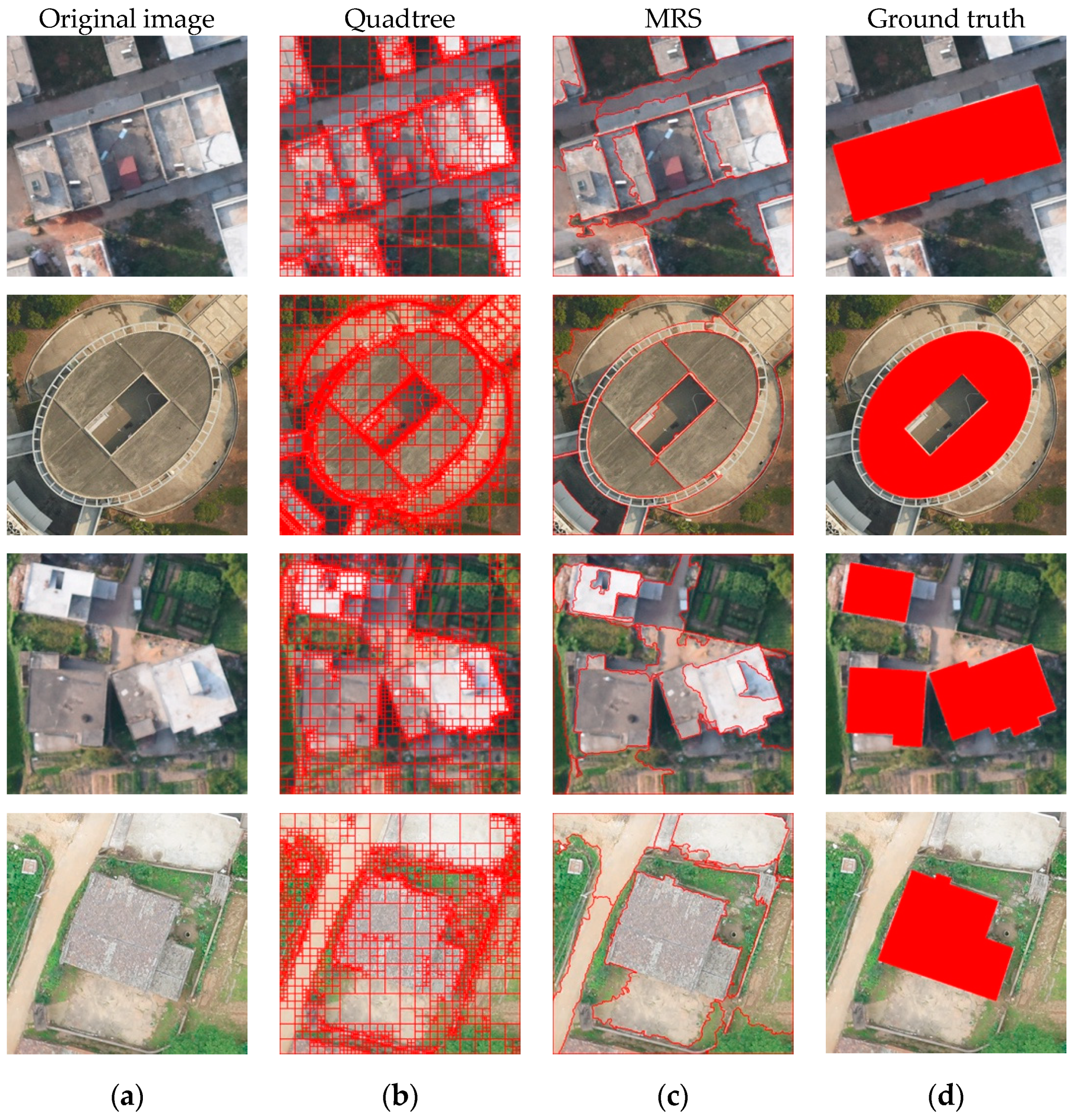
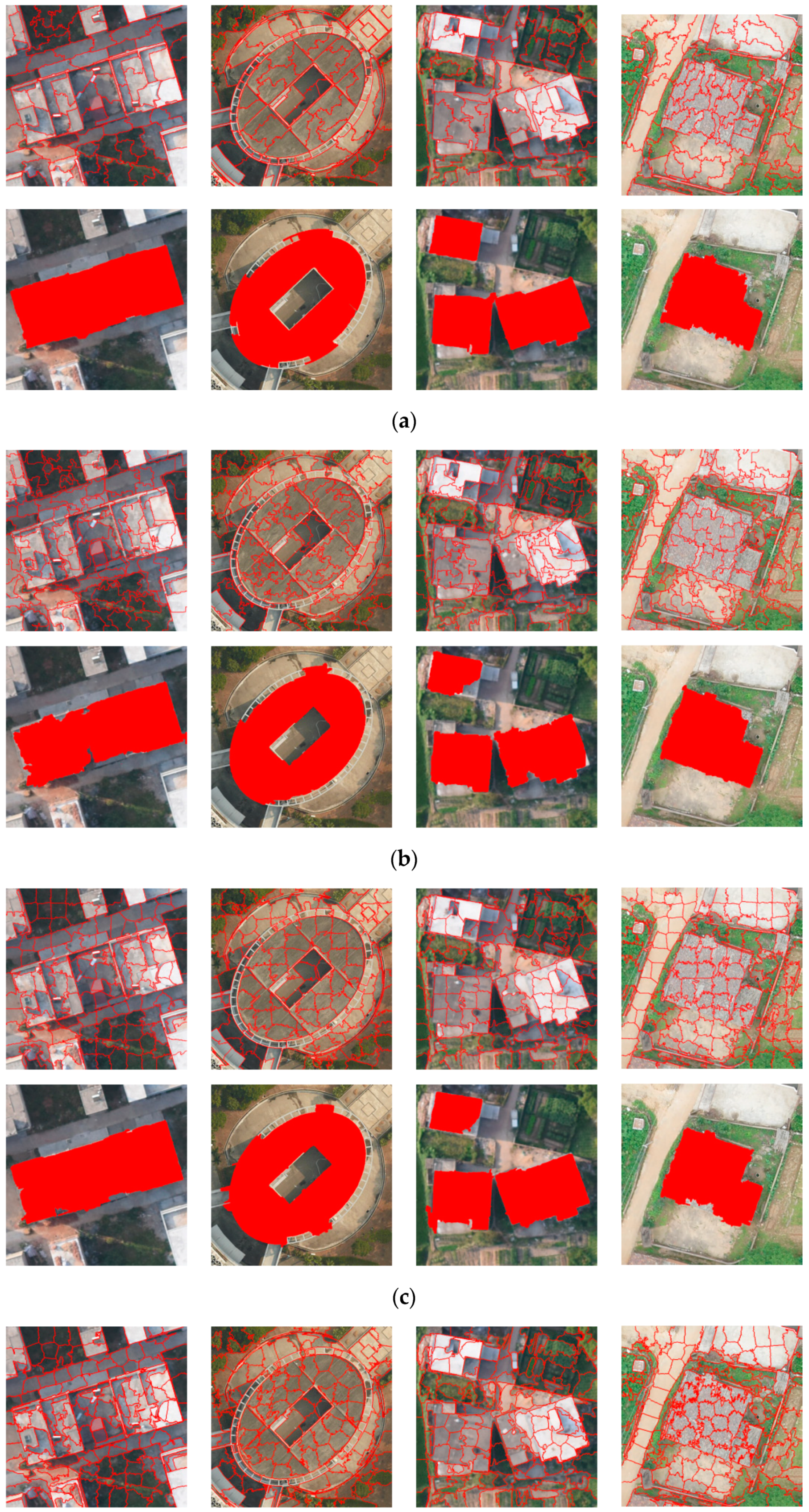
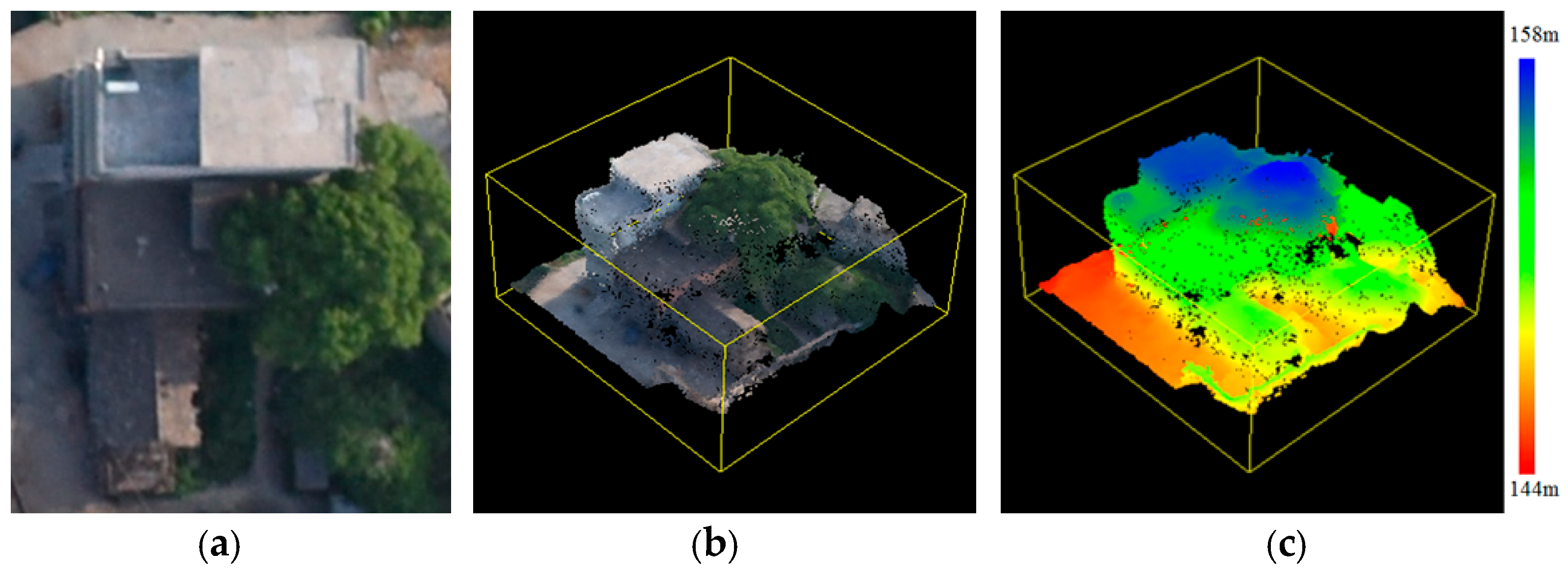
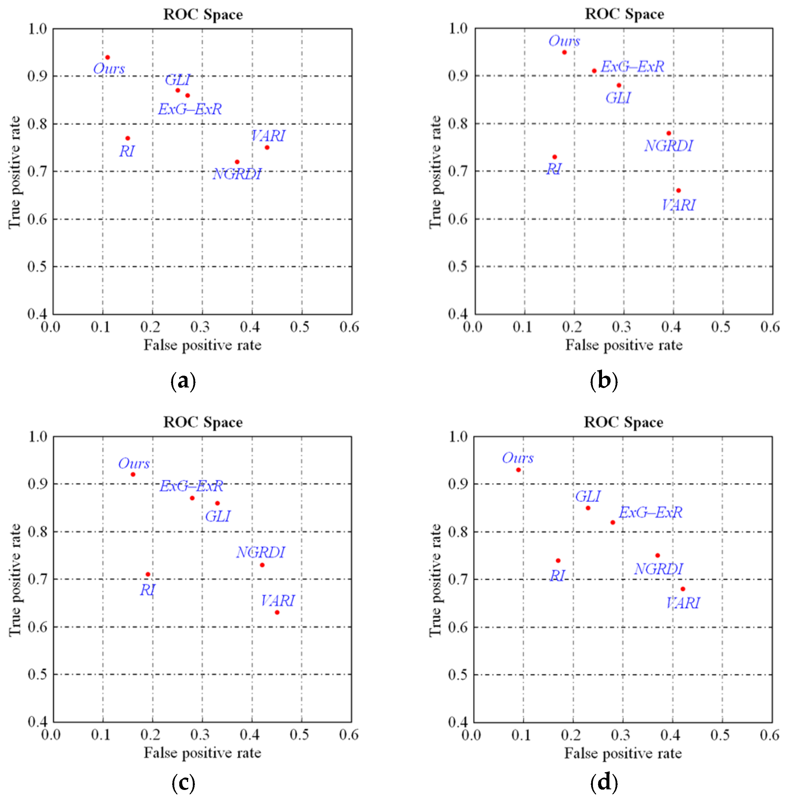
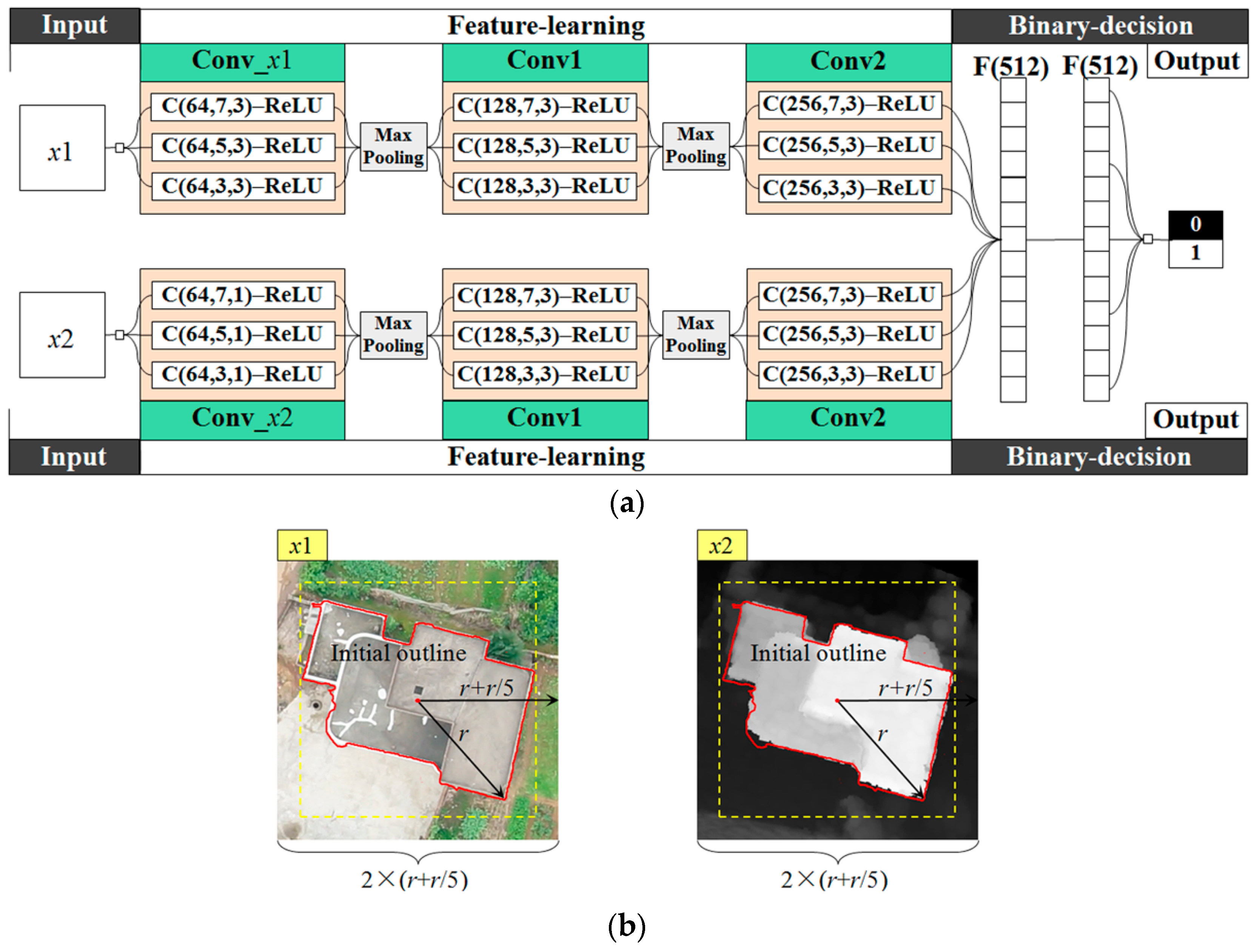
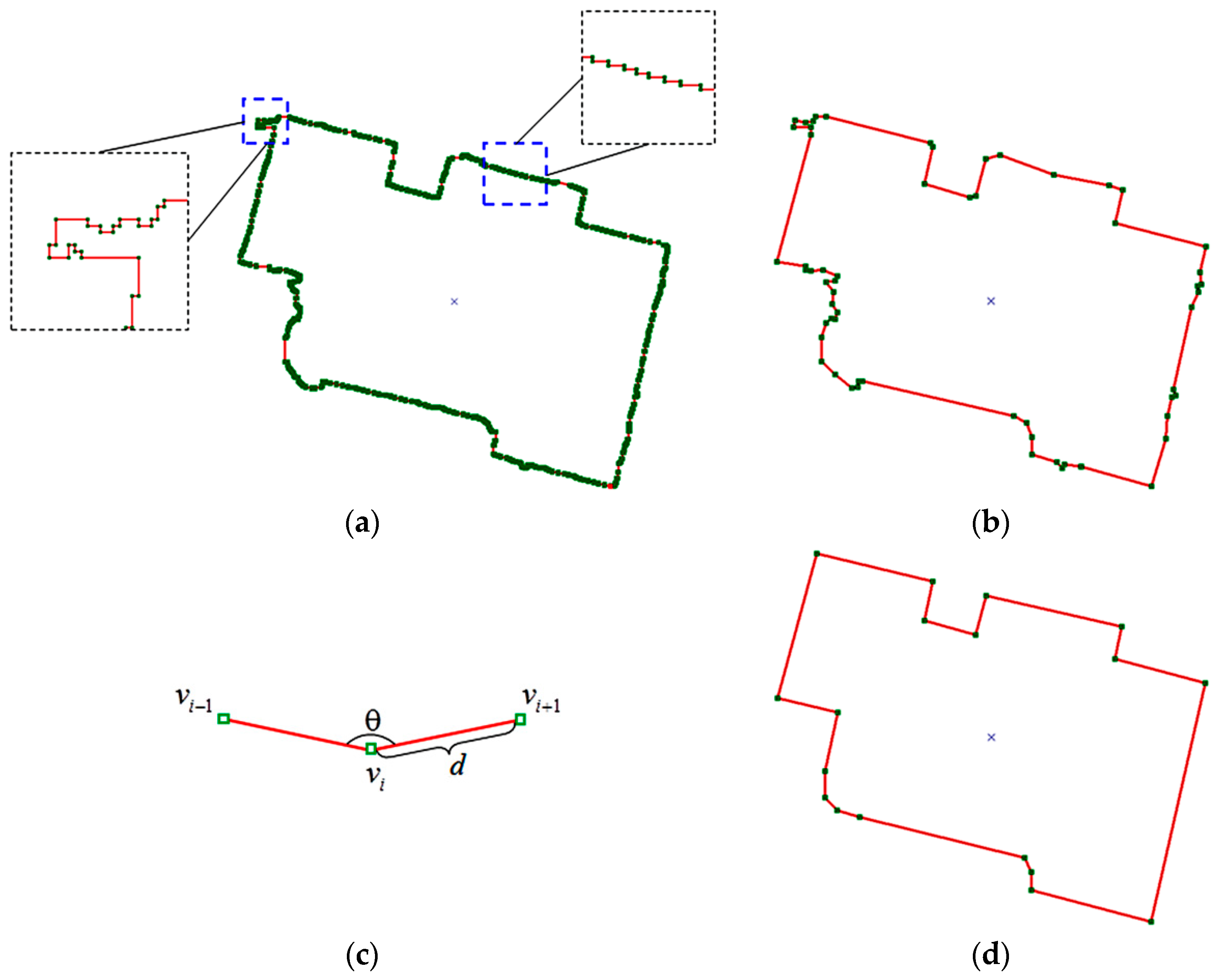
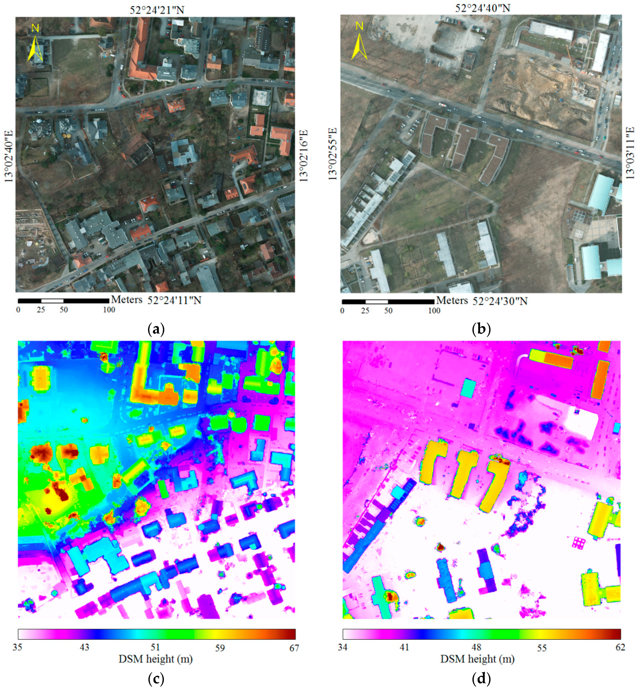
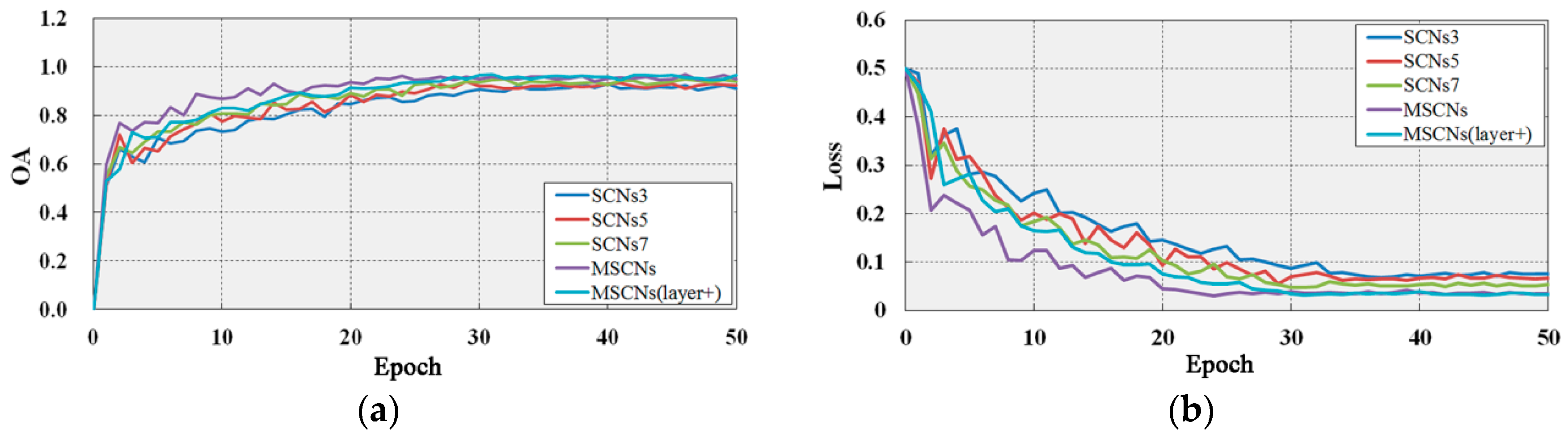
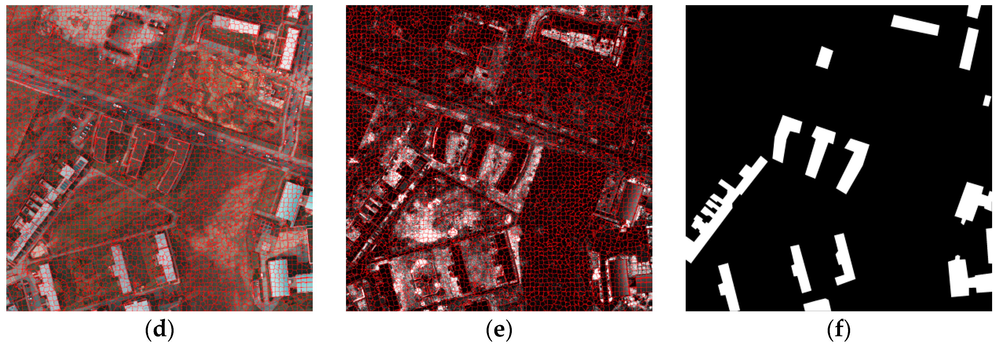
Table 1.
and values of SLIC, ERS, SEEDS, preSLIC, LSC, and 6D-SLIC in the four images in Figure 2a.
Table 1.
and values of SLIC, ERS, SEEDS, preSLIC, LSC, and 6D-SLIC in the four images in Figure 2a.
| Dataset | Metric | SLIC | ERS | SEEDS | preSLIC | LSC | 6D-SLIC |
|---|---|---|---|---|---|---|---|
| (1) | 0.7487 | 0.7976 | 0.7161 | 0.8539 | 0.9039 | 0.9076 | |
| 0.0412 | 0.0640 | 0.0378 | 0.0450 | 0.0385 | 0.0231 | ||
| (2) | 0.7152 | 0.6419 | 0.7070 | 0.5769 | 0.8443 | 0.9286 | |
| 0.1038 | 0.1213 | 0.1027 | 0.1407 | 0.0654 | 0.0443 | ||
| (3) | 0.7323 | 0.8597 | 0.8608 | 0.8669 | 0.8912 | 0.9629 | |
| 0.0681 | 0.0415 | 0.0522 | 0.0539 | 0.0625 | 0.0311 | ||
| (4) | 0.7323 | 0.7918 | 0.8810 | 0.8410 | 0.9313 | 0.9795 | |
| 0.0712 | 0.0304 | 0.0413 | 0.0497 | 0.0395 | 0.0325 |
Table 2.
Metrics of MSCNs, including , , , and .
| Model | Dataset | OA | |||
|---|---|---|---|---|---|
| SCNs3 | Training | 0.9232 | 0.9349 | 0.8674 | 0.9295 |
| Test | 0.8824 | 0.9230 | 0.8219 | 0.9044 | |
| SCNs5 | Training | 0.9440 | 0.9584 | 0.9069 | 0.9515 |
| Test | 0.9088 | 0.9385 | 0.8577 | 0.9246 | |
| SCNs7 | Training | 0.9530 | 0.9686 | 0.9244 | 0.9610 |
| Test | 0.9226 | 0.9553 | 0.8844 | 0.9397 | |
| MSCNs | Training | 0.9670 | 0.9796 | 0.9479 | 0.9735 |
| Test | 0.9584 | 0.9689 | 0.9298 | 0.9638 | |
| MSCNs(layer+) | Training | 0.9672 | 0.9798 | 0.9483 | 0.9736 |
| Test | 0.9594 | 0.9693 | 0.9311 | 0.9645 |
Table 3.
Parameters of Random Forest classifier. SIFT denotes the feature detected by using scale-invariant feature transform. Hog denotes the feature represented by using a feature descriptor, namely, histogram of oriented gradients.
Table 3.
Parameters of Random Forest classifier. SIFT denotes the feature detected by using scale-invariant feature transform. Hog denotes the feature represented by using a feature descriptor, namely, histogram of oriented gradients.
| Feature | Parameters | Description |
|---|---|---|
| Color histogram | quantization_level = 8 | Level of quantization is applied to each image. |
| color_space = “lab” | Image is converted into lab color space. | |
| Bag of SIFT | vocab_size = 50 | Vocabulary size is set as 50. |
| dimension = 128 | Dimension of descriptor is set as 128. | |
| smooth_sigma = 1 | Sigma for Gaussian filtering is set as 1. | |
| color_space = “grayscale” | Image is converted into grayscale. | |
| Hog | vocab_size = 50 | Vocabulary size is set as 50. |
| cell_size = 8 | Cell size is set as 8. | |
| smooth_sigma = 1 | Sigma for Gaussian filtering is set as 1. | |
| color_space = “rgb” | RGB color space is used. |
Table 4.
Superpixel-based building extraction results on the four datasets before regularization stage.
Table 4.
Superpixel-based building extraction results on the four datasets before regularization stage.
| Dataset | Metric | SLIC | ERS | SEEDS | preSLIC | LSC | Ours |
|---|---|---|---|---|---|---|---|
| Dataset1 | 0.8833 | 0.8933 | 0.8803 | 0.9113 | 0.9153 | 0.9421 | |
| 0.8927 | 0.9027 | 0.9127 | 0.8977 | 0.9143 | 0.9650 | ||
| 0.7986 | 0.8148 | 0.8119 | 0.8256 | 0.8430 | 0.9109 | ||
| Dataset2 | 0.8994 | 0.9094 | 0.8964 | 0.9304 | 0.9315 | 0.9583 | |
| 0.8907 | 0.9107 | 0.8804 | 0.8960 | 0.9220 | 0.9675 | ||
| 0.8001 | 0.8349 | 0.7991 | 0.8397 | 0.8635 | 0.9285 | ||
| Dataset3 | 0.8104 | 0.8204 | 0.8077 | 0.8414 | 0.8425 | 0.8890 | |
| 0.8213 | 0.8413 | 0.8111 | 0.8266 | 0.8526 | 0.9286 | ||
| 0.6889 | 0.7105 | 0.6798 | 0.7152 | 0.7354 | 0.8321 | ||
| Dataset4 | 0.8317 | 0.8417 | 0.8280 | 0.8667 | 0.8628 | 0.9016 | |
| 0.8446 | 0.8476 | 0.8448 | 0.8493 | 0.8754 | 0.9101 | ||
| 0.7213 | 0.7311 | 0.7187 | 0.7512 | 0.7684 | 0.8279 |
Table 5.
Superpixel-based building extraction results on the four datasets after regularization stage.
Table 5.
Superpixel-based building extraction results on the four datasets after regularization stage.
| Dataset | Metric | SLIC | ERS | SEEDS | preSLIC | LSC | Ours |
|---|---|---|---|---|---|---|---|
| Dataset1 | 0.9233 | 0.9243 | 0.8943 | 0.9223 | 0.9233 | 0.9611 | |
| 0.8969 | 0.9167 | 0.9237 | 0.9119 | 0.9273 | 0.9656 | ||
| 0.8347 | 0.8527 | 0.8328 | 0.8468 | 0.8609 | 0.9293 | ||
| Dataset2 | 0.9194 | 0.9364 | 0.9165 | 0.9514 | 0.9495 | 0.9683 | |
| 0.8929 | 0.9227 | 0.8944 | 0.9102 | 0.9330 | 0.9679 | ||
| 0.8281 | 0.8683 | 0.8270 | 0.8698 | 0.8889 | 0.9382 | ||
| Dataset3 | 0.8334 | 0.8474 | 0.8278 | 0.8624 | 0.8605 | 0.9190 | |
| 0.8393 | 0.8533 | 0.8251 | 0.8408 | 0.8636 | 0.9406 | ||
| 0.7187 | 0.7396 | 0.7042 | 0.7413 | 0.7575 | 0.8740 | ||
| Dataset4 | 0.8577 | 0.8687 | 0.8421 | 0.8897 | 0.8838 | 0.9416 | |
| 0.8756 | 0.8696 | 0.8638 | 0.8675 | 0.9045 | 0.9321 | ||
| 0.7645 | 0.7685 | 0.7434 | 0.7833 | 0.8084 | 0.8876 |
Table 6.
, , and values of Dai’ s method, FCN, U-Net, and our method in the four datasets.
| Dataset | Metric | Dai | FCN | U-Net | Ours |
|---|---|---|---|---|---|
| Dataset1 | 0.7931 | 0.9306 | 0.9523 | 0.9611 | |
| 0.9301 | 0.8593 | 0.9547 | 0.9656 | ||
| 0.7485 | 0.8075 | 0.9112 | 0.9293 | ||
| Dataset2 | 0.7971 | 0.9484 | 0.9566 | 0.9683 | |
| 0.9505 | 0.9533 | 0.9587 | 0.9679 | ||
| 0.7653 | 0.9063 | 0.9187 | 0.9382 | ||
| Dataset3 | 0.7471 | 0.8684 | 0.8836 | 0.9190 | |
| 0.8805 | 0.8833 | 0.9005 | 0.9406 | ||
| 0.6783 | 0.7790 | 0.8050 | 0.8740 | ||
| Dataset4 | 0.7431 | 0.8506 | 0.8793 | 0.9416 | |
| 0.8601 | 0.7893 | 0.8965 | 0.9321 | ||
| 0.6630 | 0.6932 | 0.7983 | 0.8876 |
© 2019 by the authors. Licensee MDPI, Basel, Switzerland. This article is an open access article distributed under the terms and conditions of the Creative Commons Attribution (CC BY) license (http://creativecommons.org/licenses/by/4.0/).
Share and Cite
MDPI and ACS Style
He, H.; Zhou, J.; Chen, M.; Chen, T.; Li, D.; Cheng, P. Building Extraction from UAV Images Jointly Using 6D-SLIC and Multiscale Siamese Convolutional Networks. Remote Sens. 2019, 11, 1040. https://doi.org/10.3390/rs11091040
AMA Style
He H, Zhou J, Chen M, Chen T, Li D, Cheng P. Building Extraction from UAV Images Jointly Using 6D-SLIC and Multiscale Siamese Convolutional Networks. Remote Sensing. 2019; 11(9):1040. https://doi.org/10.3390/rs11091040
Chicago/Turabian StyleHe, Haiqing, Junchao Zhou, Min Chen, Ting Chen, Dajun Li, and Penggen Cheng. 2019. "Building Extraction from UAV Images Jointly Using 6D-SLIC and Multiscale Siamese Convolutional Networks" Remote Sensing 11, no. 9: 1040. https://doi.org/10.3390/rs11091040
Note that from the first issue of 2016, this journal uses article numbers instead of page numbers. See further details here.