Upstream Remotely-Sensed Hydrological Variables and Their Standardization for Surface Runoff Reconstruction and Estimation of the Entire Mekong River Basin

Abstract

River water discharge (WD) is an essential component when monitoring a regional hydrological cycle. It is expressed in terms of surface runoff (R) when a unit of river basin surface area is considered. To compensate for the decreasing number of hydrological stations, remotely-sensed WD estimation has been widely promoted over the past two decades, due to its global coverage. Previously, remotely-sensed WD was reconstructed either by correlating nearby remotely-sensed surface responses (e.g., indices and hydraulic variables) with ground-based WD observations or by applying water balance formulations, in terms of R, over an entire river basin, assisted by hydrological modeling data. In contrast, the feasibility of using remotely-sensed hydrological variables (RSHVs) and their standardized forms together with water balance representations (WBR) obtained from the river upstream to reconstruct estuarine R for an entire basin, has been rarely investigated. Therefore, our study aimed to construct a correlative relationship between the estuarine observed R and the upstream, spatially averaged RSHVs, together with their standardized forms and WBR, for the Mekong River basin, using estuarine R reconstructions, at a monthly temporal scale. We found that the reconstructed R derived from the upstream, spatially averaged RSHVs agreed well with the observed R, which was also comparable to that calculated using traditional remote sensing data (RSD). Better performance was achieved using spatially averaged, standardized RSHVs, which should be potentially attributable to spatially integrated information and the ability to partly bypass systematic biases by both human (e.g., dam operation) and environmental effects in a standardized form. Comparison of the R reconstructed using the upstream, spatially averaged, standardized RSHVs with that reconstructed from the traditional RSD, against the observed R, revealed a Pearson correlation coefficient (PCC) above 0.91 and below 0.81, a root-mean-squares error (RMSE) below 6.1 mm and above 8.5 mm, and a Nash–Sutcliffe model efficiency coefficient (NSE) above 0.823 and below 0.657, respectively. In terms of the standardized water balance representation (SWBR), the reconstructed R yielded the best performance, with a PCC above 0.92, an RMSE below 5.9 mm, and an NSE above 0.838. External assessment demonstrated similar results. This finding indicated that the standardized RSHVs, in particular its water balance representations, could lead to further improvement in estuarine R reconstructions for river basins affected by various systematic influences. Comparison between hydrological stations at the Mekong River Delta entrance and near the estuary mouth revealed tidally-induced backwater effects on the estimated R, with an RMSE difference of 4–5 mm (equivalent to 9–11% relative error).

1. Introduction

River water discharge (WD) is an important water balance component of the hydrological cycle. It is defined as the water volume rate passing through a cross-section of a river and is expressed in terms of surface runoff (R) when a unit of surface area over a river basin is considered [1]. Its monitoring is essential for increased water management efficiency and tracking the regional hydrological extremes (i.e., droughts and floods) that cause unpredictable losses to agriculture and economy [2,3,4,5]. Thus, continuous WD time series data are necessary within a river basin.

Traditionally, WD has been directly measured at hydrological stations along a river. However, due to the varied politics, economies, and topography of the countries along a river [6], the spatial distribution of hydrological stations is uneven and sparse. In addition, acquisition of discharge data and their entry into a database has been declining since the late 1970s [7]. A lack of funding to continuously operate and maintain WD data systems is one of the reasons for this decline, therefore, new, indirect methods for observing WD are gaining increased attention.

Several research studies have investigated potential remotely sensed WD estimation, based on recent advances in remote sensing (RS). RS techniques can be divided into two types, passive and active. Moderate Resolution Imaging Spectrometer (MODIS), Landsat Thematic Mapper (TM), and Enhanced TM Plus (ETM+) are examples of passive RS techniques, which measure instantaneous surface response parameters, such as water surface area, floodplain inundation, the Normalized Difference Vegetation Index (NDVI), and Land Surface Temperature (LST) [8,9,10,11]. These passive remote sensing data (RSD) have been directly correlated with water level (WL) or WD [12,13,14] and applied to several river basins over the past two decades [15,16,17]. However, these data are not hydrological quantities with direct causal relationships to WD.

As well as these passive RS quantities, remotely sensed hydraulic variables have been used as inputs to infer WD through hydraulic geometry (e.g., [18,19]). For instance, WD can be inferred by integrating remotely-sensed hydraulic variables with topographic information (e.g., DEM), through well-known hydraulic models, such as Manning’s equation (e.g., [20,21,22,23,24]). An innovative functional relationship between discharge and river width has been established recently, using hydraulic geometry for WD estimation [25,26]. Novel procedures that optimize the unknown parameters in the modified Manning’s equation have also been developed [27]. Nevertheless, the accuracy of the estimated WD is region-dependent, relating to detection ability with respect to small changes in river width [28] and the availability of roughness coefficients for some regions [29,30].

Satellite radar altimetry is one of the active RS techniques that can directly measure water level (WL) fluctuations over inland lakes and rivers (e.g., [31,32]). Since WL is a power function of WD (e.g., [33,34]), active, remotely sensed WD mainly correlates the measured satellite altimetric WL of a river with ground-based WD measurements (e.g., [35]). In addition to estimating WD using satellite ground tracks, a basin-wide WD estimation for the Mekong River Basin (MRB) has been demonstrated, through multi-satellite altimetric (e.g., ERS-2 and Envisat) WL data [36]. To improve the temporal resolution of WD estimation, multi-altimetry data have been assimilated into hydrodynamic (e.g., [37]) or dynamic stochastic process models, using Kalman filtering to estimate WD [38]. In addition, WD estimation based on satellite altimetric sea level anomaly data near the estuary has been demonstrated [39]. However, the accuracy of the satellite radar altimetry technique is limited by the size of its footprint (i.e., 5 km, 20 km, and 3.4 km for TOPEX, ERS-2, and Envisat satellites, respectively) and because radar signals are contaminated by land surfaces near the riverbank when river width is small (e.g., [40]).

The Gravity Recovery and Climate Experiment (GRACE) [41] is another active RS technique that has used large-scale, time-variable gravity changes to infer monthly terrestrial water storage (TWS) fluctuations (e.g., [42,43]). GRACE TWS is useful for capturing large-scale, seasonal surface water changes, which in turn allows monitoring of the global hydrological cycle and its extremes (e.g., [44,45]). Since WD is a power function of GRACE TWS (S) (e.g., [46,47]), WD can be inferred from S. Another approach to infer WD is based on the water balance equation (i.e., $R=P-ET-\Delta S$) [48,49,50], where WD is in the form of surface runoff (R) to be consistent with the units of precipitation (P), evapotranspiration (ET), and water storage change (ΔS). In addition, parameters S and ΔS are useful for inferring both precipitation (P) (e.g., [51]) and evapotranspiration (ET) (e.g., [52,53]).

These hydrological variables—P, ET, S, and R—are the four water balance components. P, ET, and S can be obtained from Tropical Rainfall Measuring Mission (TRMM), MODIS, and GRACE, respectively. These variables are referred to as remotely-sensed hydrological variables (RSHVs), while R can only be indirectly inferred. In essence, remotely-sensed P, ET, and S should have a direct causal relationship with R, and their standardized forms, which can be obtained through the subtraction of the data time series from the corresponding mean, divided by the corresponding standard deviation, should make their averaged time series more representative of regional characteristics [54]. This is particularly the case across regions with large differences in means and variances [55,56], reducing the systematic environmental influences [57]. RSHVs and their standardized forms are presumably better at capturing variations of R and standardized R, respectively, through direct correlative analysis, though standardized hydrological variables have been traditionally applied to drought characterization [58,59]. Since R inferred from the water balance equation is achieved through subtraction among the RSHVs, systematic biases due to both human (e.g., dam operation) and environmental influences should be reduced, and thus, the inferred R from the water balance equation could be expected to outperform the correlative analysis of each individual RSHV, not to mention the inferred R from the standardization of the water balance equation (i.e., $SRI=SPI-SETI-\Delta SI$). These two forms are referred to as water balance representations (WBR).

The Mekong River Delta (MRD), close to the estuary mouth where there are several river mouths, is crucial for the food (e.g., fish and agriculture products [60]) and water (e.g., [61]) security of Southeast Asia, making it an attractive geographic study region. However, the upper Mekong River Basin (MRB) has been undergoing massive hydropower development since the 1990s, with the aim of regulating R during severe flood and drought periods [62,63]. As a consequence, modification of the upstream R due to dam operation could well pose severe downstream impacts at different times and seasons of the year (e.g., [64,65,66]), extending down to the MRD. In essence, the effect of dam operation in the upstream MRB propagates and accumulates with the effects of other dams along the mainstream Mekong River until reaching the MRD, where the accumulated effect detected in the MRD should be approximately similar for any specific month, year-on-year [66]. This accumulated effect, including ice and snowmelt water in the upper MRB [67], should be partly systematic, based on the dam operation principle of increasing (decreasing) discharge in dry (wet) seasons, with little overall change to annual flow.

These reasons support our investigation into the feasibility of using RSHVs, their standardized forms, as well as water-balance representations (WBR) obtained from the upstream MRB to reconstruct time series of R in the MRD at a monthly temporal scale. We can proceed on this basis. since the above standardization procedure (i.e., $R_{i,j}-median\left(R_j\right)$), and subtraction in WBR (i.e.,$S_{i+1,j}-S_{i,j}$), can mitigate the systematic bias introduced by dam operations and other environmental influences. The reconstructed relationship can be externally validated by estimating the time series of R at other locations in the MRD, with in situ station time series used for performance assessment. The commonly available RSD (i.e., NDVI [68] and LST [69]) can also serve as baseline results for comparison purposes.

The paper has been organized as follows: In Section 2, the geography of the MRB and of Yunnan Province in China have been presented. Datasets are described in Section 3, which is followed by methodology and evaluation metric descriptions in Section 4. In Section 5, reconstruction and estimation of R based on RSHVs, their standardized forms, and WBR, have been investigated and then compared with NDVI and LST results. Finally, conclusions have been given in Section 6.

2. The Geography of the Mekong River Basin (MRB) and of Yunnan Province

The Mekong River, originating from the northeast slopes of the Tanggula Mountains, China, is the 12th longest river in the world, with a main stream total length of 4909 km [70]. The river first flows as the Lancang River (also called the Mekong River outside of China) in Yunnan Province, China, before making its way through Laos, Myanmar, Thailand, Cambodia, and Vietnam. These six countries constitute the entire MRB, which covers an area of ~795,000 km², spanning 25° of latitude [71] (Figure 1).

Located at the center of the Asian tropical monsoon region, the MRB, particularly in its lower reaches, is significantly influenced by the Asia–Pacific monsoon system [72]. The MRB rainy season extends from May to October and is controlled by the Southwest (SW) monsoon from the ocean, while the dry season, which lasts from November to April, is greatly influenced by the Northeast (NE) monsoon from the mainland [73]. It is noted that, apart from a small portion of ice and snowmelt water flowing from upstream, rainfall is the dominant R component within the basin [74]. The water cycle consists of downstream R rising abruptly in May, before peaking in late September during the rainy season, then decreasing from November and reaching its lowest level in April during the dry season [73], illustrating that R for the entire MRB is greatly affected by monsoon behavior.

Yunnan Province, with mountainous plateau topography descending stepwise from north to south [75], is the main upstream MRB area. It is located in SW China, with an extent of 21°–29° N latitude, and 97°–106° E longitude (Figure 1). It has an area of 394,100 km² and is inhabited by 47.7 million people [76]. It has a subtropical plateau monsoon climate that is jointly influenced by the SW and SE warm, moist air flows. Precipitation is distributed non-uniformly across the province, both in terms of space and time. The rainy and dry seasons are distinct, with the former (May–October) accounting for 85% of the annual rainfall [77].

3. Datasets

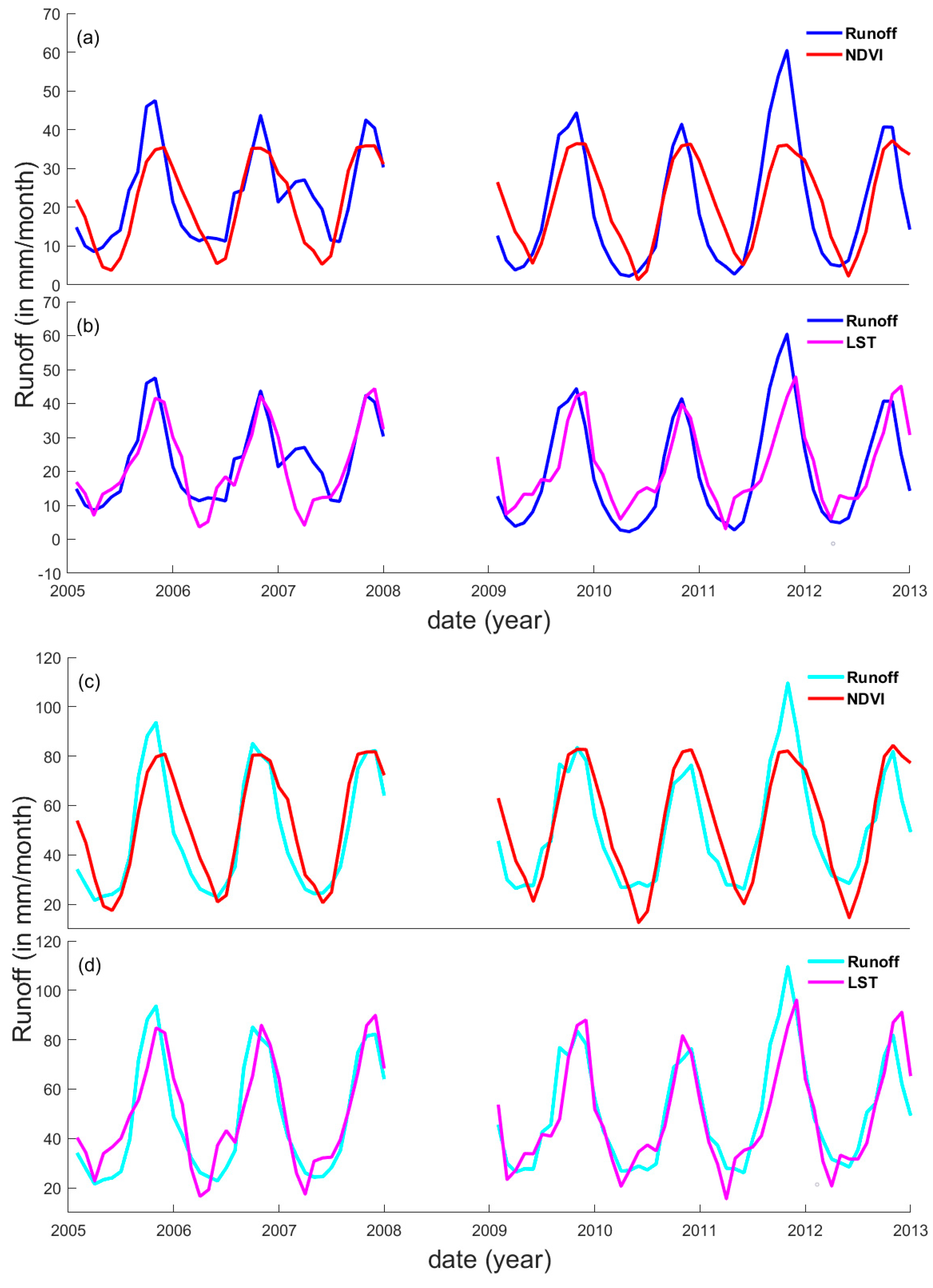
3.1. In Situ Hydrological Stations and Traditional Remotely-Sensed Data

Based on its discharge variability, the geographic setting of the MRD study site belongs to a fluvial to marine transition zone, where it is dynamically affected by a combination of fluvial and marine (i.e., tide and wave) processes that varies seasonally [78,79]. It is linked to a complicated river system, where the total discharge of the MRB is regulated by Cambodia’s Tonle Sap Lake (e.g., [80,81,82]) before delivering to the MRD and discharging to the South China Sea (SCS) through several distributaries associated with the two main branches, the Bassac River and the Mekong River. This system is complicated by oceanic tidal propagation landward from the estuary mouth [60], and consequently, selection of the most appropriate hydrological stations is critical.

Given the above setting, the MRD hydrological stations to be used in this study had to be selected at locations where the regulating effects of Tonle Sap Lake and the ocean tides close to estuary were minimized. The Chaktomuk station at Phnom Penh is ~300 km away from the estuary mouth, at the intersection of several main distributaries. When river flows from where several main distributaries meet, the overall temporal pattern of discharge of the MRB mainstream could be altered, and so this station was not selected.

Given the above criteria, Tan Chau and Chau Doc, located at the MRD entrance, approximately 220 km from the estuary mouth and on the edge of the fluvial to marine transition zone [79], were considered to be the most appropriate hydrological stations. They were considered to be far enough away from the river mouth for the ocean tidal propagation effect to be reduced (Figure 1). Note that semi-diurnal (i.e., half-daily period) ocean tides are dominant in the SCS, and that ocean tidal influence can be mitigated by adopting a monthly averaging process. Therefore, the two stations above were chosen in this study. The Can Tho and My Thuan stations, closest to the estuary mouth, were also chosen to assess the impact of the backwater effect, caused by landward ocean tidal propagation, on surface runoff estimation.

Station data were obtained from the Mekong River Commission (MRC) (http://www.mrcmekong.org). In order to reduce the effect of newly constructed dams in Yunnan Province (e.g., Nuozhadu Dam, which went online in September 2012), the station WD time series data spanning January 2005 to December 2012 were generally selected, to be consistent with the RSD time span. To convert the observed WD (in m³/s) into a daily R rate (in mm/day) per unit area over the MRB, the observed WD was divided by the approximate total MRB drainage area (i.e., 795,000 km²). This allowed a monthly R rate (in mm/month) to be calculated for the entire MRB by summing the daily R rates. As mentioned above, WD is a power function of WL, so too the R. The specific relationship between WL and R for the four selected stations, is given in Figure 2, and basic observed data—maxima, minima, means, and standard deviations—are provided in

Table 1. Water discharge (1 × 10⁴ m³/s), water level (m), and runoff (mm/month) maxima, minima, means, and standard deviations for the four selected Mekong River Delta hydrological stations.

Variable	Station	Maximum	Minimum	Mean	Standard Deviation
Water Discharge (1 × 104 m3/s)	My Thuan	1.854	0.069	0.661	0.449
	Can Tho	1.950	0.081	0.692	0.446
	Tan Chau	3.362	0.661	1.528	0.696
	Chau Doc	3.178	0.683	1.375	0.568
Water Level (m)	My Thuan	7.613	1.770	4.522	1.509
	Can Tho	4.380	1.714	3.072	0.655
	Tan Chau	8.481	0.501	3.688	1.785
	Chau Doc	7.802	0.244	2.923	1.449
Runoff (mm/month)	My Thuan	60.5	2.2	21.6	14.6
	Can Tho	63.6	2.6	22.5	14.6
	Tan Chau	109.6	21.6	49.8	22.7
	Chau Doc	103.6	22.3	44.8	18.5

.

Regardless of which station pair (My Thuan and Can Tho or Tan Chau and Chau Doc) were studied, the pairs’ time series results were very similar and shared the same periodicities, despite differences in R peaks and troughs (Figure 3). Note that data were missing for the My Thuan and Can Tho station pair from January until December 2008, and so, to be consistent, the entire data of year 2008 for the station pair of Tan Chau and Chau Doc were not used.

Consistent with the descriptions in Section 2, the yearly peak and trough appear in September and April, respectively. Anomalies from February to June 2007 could be noticed for the station pair of My Thuan and Can Tho, and we speculated that the backwater effect due to ocean tides might have been intensified at this time due to local drought. No such anomaly was observed for the station pair of Tan Chau and Chau Doc.

Traditional MODIS remotely-sensed data (RSD) products (i.e., NDVI from MOD13C2, and LST from MOD11C3 data products) are accessible from the Land Processes Distribution Active Archive Center (LP DAAC) under the auspices of the NASA Earth Science Data and Information System (ESDIS) (https://lpdaac.usgs.gov/dataset_discovery/modis/modis_products_table). Both data sets were used for baseline information, to compare against R reconstructions.

3.2. Remotely-Sensed Hydrological Variables and Their Standardization

Based on the water balance concept, four kinds of hydrological variables—precipitation, evapotranspiration, water storage, and surface runoff—are described in Section 1. Accessible hydrological variable data resources are described in this section. All data, except as specified from the above and missing data, covered a time window spanning from January 2005 to December 2012, with information available at monthly sampling intervals.

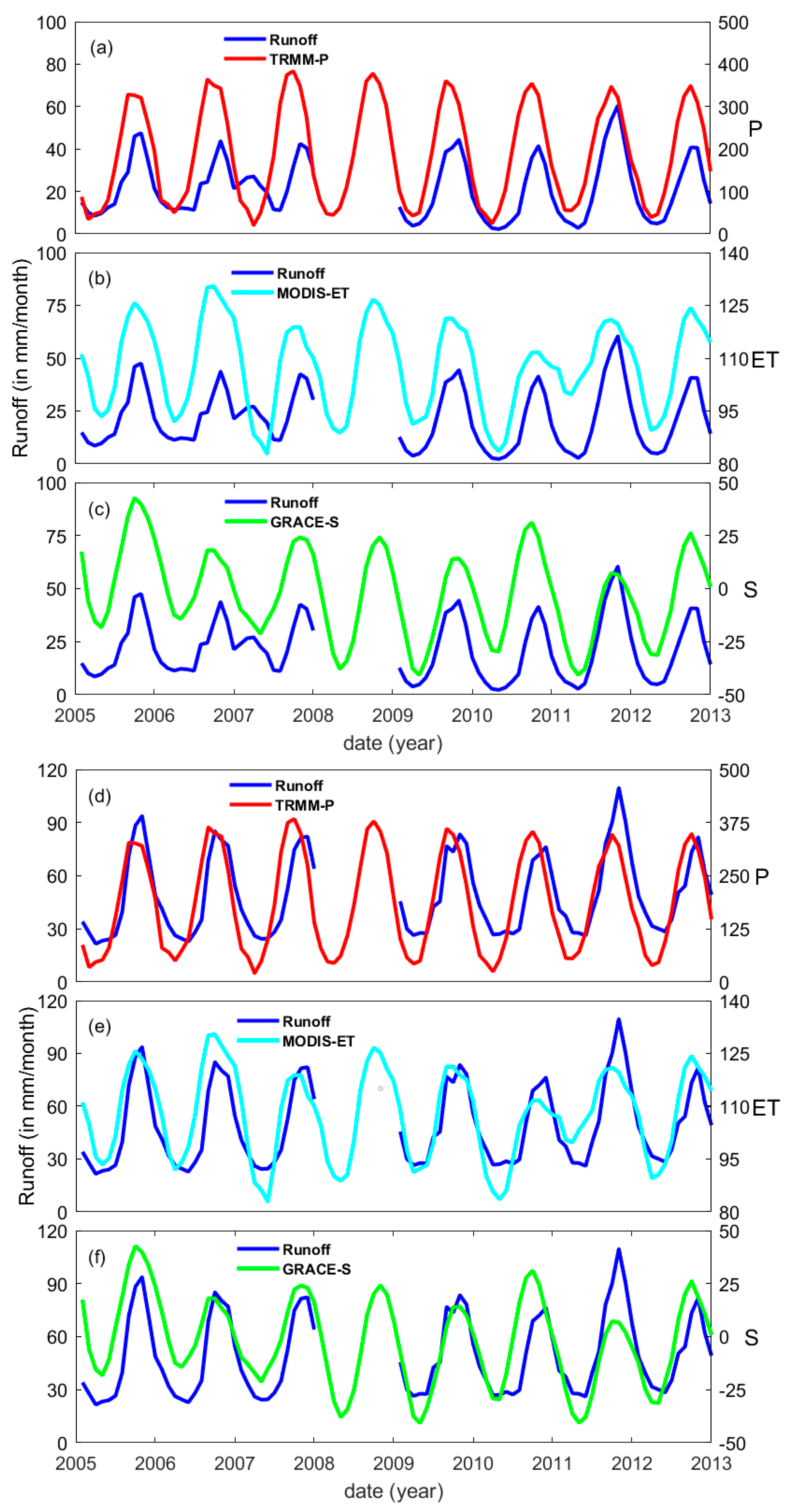
3.2.1. Remotely-Sensed Precipitation and Its Standardized Index, from TRMM

TRMM is a meteorological satellite mission exclusively responsible for quantifying spatio-temporal rainfall variation in the tropical and the subtropical regions [83]. Monthly global precipitation data were derived from TRMM Rainfall Estimate L3 (TRMM_3B43 V7), with a spatial resolution of 0.25°. These data sets are available from the Goddard Earth Sciences Data and Information Services Center (GES DISC) managed by NASA (https://mirador.gsfc.nasa.gov/).

The Standardized Precipitation Index (SPI) was developed by McKee et al. [84] and has a better ability to represent precipitation deficits at different time scales. Since precipitation is temporally discrete in any one region (and does not occur every day), SPI requires a special calculation based on the standardization of cumulative probability distribution [85] (equations have not been shown since this is a well-known index).

Hence, SPI was calculated for the period 1998–2012, using the TRMM monthly precipitation data product, while extracting the calculated values between 2005 and 2012. Though a 30-year continuous precipitation time series would be preferable for climatic study, the current TRMM data time span was considered sufficient for hydrological study.

3.2.2. Remotely-Sensed Terrestrial Water Storage (TWS) and Its Standardized Index, from GRACE

GRACE, a joint project of NASA and Deutsches Zentrumfür Luft- und Raumfahrt (DLR), is a satellite mission that measures time-variable changes of the Earth’s gravity field, thereby enabling TWS variation monitoring at the global scale. TWS data, with the spatial resolution of 1°, were computed from the CSR GRACE Level-2 Release 05 (RL05) GSM monthly gravity fields, in the form of spherical harmonic coefficients, up to degree 60. These data are freely accessible from the Center of Space Research (CSR) managed by NASA (http://www2.csr.utexas.edu/grace/RL05.html).

Note that two post-processing steps were applied to the GRACE gravity spherical harmonic coefficients to derive the TWS data. First, the GRACE C₂₀ term was replaced by Satellite Laser Ranging (SLR), and degree-one terms were restored to correct for geocenter motion [86,87]. Second, a de-striping process and Gaussian filtering with a radius of 350 km were applied to reduce the spatially correlated error of TWS data at higher degrees [88,89].

The derived monthly GRACE TWS (S) were utilized to: (i) correlate directly with the ground-based observed R and (ii) calculate a newly proposed GRACE drought severity index (i.e., GRACE-SI), followed by correlating with the standardized R.

To characterize abrupt TWS changes and drought events, GRACE-SI is a recently-derived drought severity index in a standardized form, proposed by Zhao et al. (2017) [90]. To reduce abnormal TWS anomalies, for each month of the entire time series, TWS anomaly medians, instead of TWS anomaly means, were used in the calculation of GRACE-SI [91], which is defined as shown in Equation (1).

$$S{I}_{i,j}=\frac{S_{i,j}-median\left(S_j\right)}{s_j}$$

(1)

In Equation (1), $S{I}_{i,j}$ and $S_{i,j}$ represent the GRACE-SI and original GRACE TWS in year i and month j, respectively, $median\left(S_j\right)$ is the median TWS value for each month, and $s_j$ is the sampled standard deviation of TWS for month j.

3.2.3. Remotely-Sensed Evapotranspiration and Its Standardized Form, from MODIS

Evapotranspiration (ET), being a total amount of water vapor transported to the atmosphere from vegetation and the land surface [92], is available from the MODIS Global Evaporation Project (MOD16A2) dataset, managed by NASA LP DAAC (https://lpdaac.usgs.gov/dataset_discovery/modis/modis_products_table). The dataset has a spatial resolution of 0.5°, from latitude 80° N to −60° N and from longitude 0° E to 360° E.

In order to capture changes in ET better, and to be consistent with the other two standardized RSHVs (i.e., SPI and SI), ET was transformed into its standardized form (called the Standardized Evapotranspiration Index (SETI)) using a similar calculation procedure, as shown in Equation (1). Hence, SETI between 2000 and 2014 was calculated while extracting the calculated values between 2005 and 2012.

4. Methodology and Evaluation Metrics

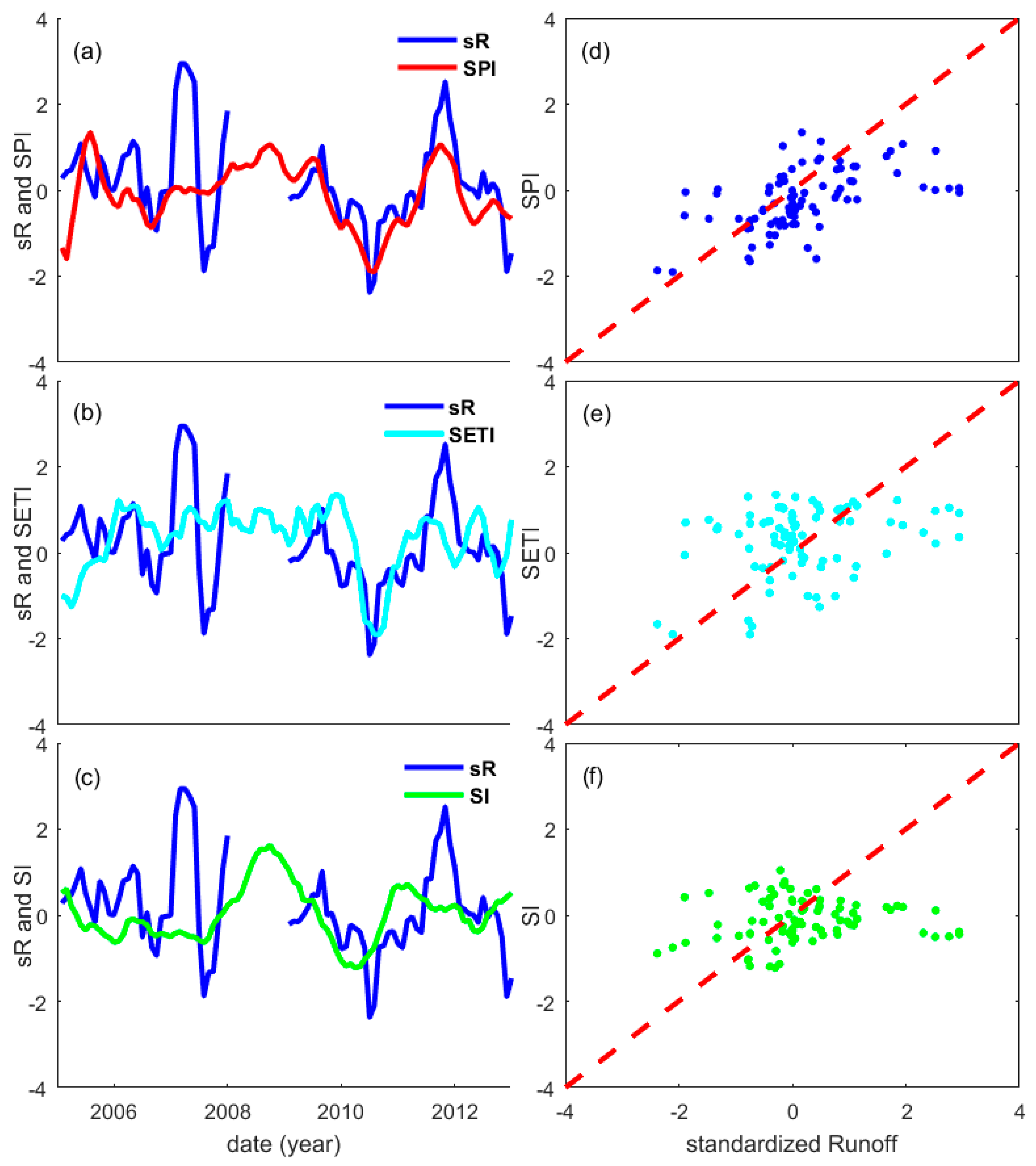
4.1. Correlative Analysis, Data Standardization Results, and Estimation Procedures

Yunnan Province, located at the upstream MRB, was selected in this study to reconstruct and estimate R in the MRD. All the RSD and RSHVs for the entire Yunnan Province were spatially averaged. In addition, a two-month time lag was observed between R and TRMM precipitation (TRMM-P) and MODIS evapotranspiration (MODIS-ET), whereas no time lag was found between R and GRACE TWS (GRACE-S) in the MRB. To reconstruct and estimate R in the MRD better [74], two additional pre-processing procedures were applied on three different RSHVs. Firstly, smoothing and re-scaling procedures were applied to RSHV before the correlative analysis was conducted, and secondly, a two-month time-lag shift was applied to TRMM-P and MODIS-ET to improve the estimated performance. This form of time lag analysis has been widely used to improve hydrological modeling (Figure 4) [93].

Since the RSD (i.e., NDVI and LST) and RSHV time series were shown to have a clear correlative relationship with the observed R at the selected stations (i.e., My Thuan and Tan Chau stations), linear regression was applied to determine the quantitative relationship between the RSD (RSHV) and the observed R during the overlapping period. The R reconstruction formula (when $R_h=1$) can be given as shown in Equation (2).

$$R_{i,j}=R_h\times \left(a+b\times D_{i,j}\right)$$

(2)

In Equation (2), $R_{i,j}$ and $D_{i,j}$ represent the reconstructed R and the RSD (RSHV) in year i and month j, respectively, and a and b are the offset and the slope obtained from regression fitting, respectively. $R_h$ is the ratio owing to the height difference between the two stations used for estimation (when $R_h\ne 1$), which can be calculated from the ETOPO1 1-arc-min global relief topography model [94].

These reconstruction procedures served as an internal performance assessment, whereas the same procedure applied to estimate R at stations other than those used for reconstruction in the MRD was referred to as an external performance assessment of the method used in this study.

To detect hydrology changes and represent regional characteristics better, the RSHVs were transformed into their standardized forms (Section 3.2) [74]. Instead of employing the sophisticated standardized runoff index (SRI) [58] that has been currently applied to renewable surface freshwater availability for agricultural products [5], the same standardization procedure was applied to R, in order to be comparable with the standardized RSHVs, for simplicity. R standardization can be achieved by using the following equation:

$$s{R}_{i,j}=\frac{R_{i,j}-median\left(R_j\right)}{s_j}$$

(3)

In Equation (3), $s{R}_{i,j}$ and $R_{i,j}$ represent the standardized and the observed runoff in year i and month j, respectively, $median\left(R_j\right)$ is the median runoff value for each month (Figure 5), and $s_j$ is the sampled runoff standard deviation for each separate month j.

High correlations between the standardized RSHVs and the standardized R are shown in Figure 6 and Figure 7.

The water balance representation of R (i.e., WBR) and its standardization (SWBR) were calculated from the three RSHVs (i.e., P, ET and S) and their standardized forms (i.e., SPI, SETI, and SI), respectively. The WBR was calculated as:

$$cWB{R}_{i,j}=P_{i,j}-E{T}_{i,j}-\Delta S_{i,j}$$

(4)

$$WB{R}_{i,j}=\frac{cWB{R}_{i,j}-median\left(cWB{R}_j\right)}{s_j}$$

(5)

In Equations (4) and (5), $P_{i,j}$ and $E{T}_{i,j}$ represent P and ET in year i and month j, respectively. $\Delta S_{i,j}$ is the difference between GRACE-S in year i, month j + 1 and year i, month j. Similarly, SWBR can be derived as shown in (6), where $SP{I}_{i,j}$ and $SET{I}_{i,j}$ represent SPI and SETI in year i and month j, respectively. $\Delta S{I}_{i,j}$ is the difference between GRACE-SI in year i, month j + 1 and year i, month j.

$$SWB{R}_{i,j}=SP{I}_{i,j}-SET{I}_{i,j}-\Delta S{I}_{i,j}$$

(6)

A correlating procedure between the standardized R and all standardized forms (e.g., standardized RSHVs, WBR, and SWBR) was applied before reconstruction and estimation. Then, the reconstructed ($R_h=1$) and estimated ($R_h\ne 1$ from values listed in Table 1 and

Table 2. Internal assessment of surface runoff (R), reconstructed using data from My Thuan station, and external assessment of R, estimated for Can Tho and Tan Chau stations. The legend ‘My Thuan estimate Can Tho’ (or ‘Tan Chau’) means that the R for Can Tho (or Tan Chau) was estimated based on the reconstructed relationships between the R from My Thuan station and the abovementioned variables.

Station	Variables		PCC	RMSE (mm)	NSE
My Thuan (Rh = 1)	Traditional RSD	NDVI	0.766	9.1	0.585
		LST	0.808	8.3	0.651
	Hydrological Variables	TRMM-P	0.773	9.0	0.603
		MODIS-ET	0.771	9.1	0.600
		GRACE-S	0.741	9.6	0.556
	Hydrological Indices	SPI	0.905	6.1	0.811
		SETI	0.903	6.2	0.808
		SI	0.897	6.3	0.799
	Water-balance Representations	WBR	0.898	6.3	0.802
		SWBR	0.910	5.9	0.822
My Thuan estimate Can Tho (Rh = 1.05)	Traditional RSD	NDVI	0.722	9.8	0.507
		LST	0.764	9.1	0.575
	Hydrological Variables	TRMM-P	0.752	9.5	0.576
		MODIS-ET	0.741	9.7	0.562
		GRACE-S	0.711	10.1	0.513
	Hydrological Indices	SPI	0.860	7.3	0.730
		SETI	0.856	7.4	0.722
		SI	0.852	7.4	0.716
	Water-balance Representations	WBR	0.854	7.3	0.725
		SWBR	0.865	7.1	0.738
My Thuan estimate Tan Chau (Rh = 2.20)	Traditional RSD	NDVI	0.813	11.7	0.576
		LST	0.867	13.1	0.668
	Hydrological Variables	TRMM-P	0.937	9.6	0.822
		MODIS-ET	0.850	14.6	0.588
		GRACE-S	0.772	15.8	0.518
	Hydrological Indices	SPI	0.923	12.2	0.714
		SETI	0.928	12.1	0.720
		SI	0.937	11.2	0.758
	Water-balance Representations	WBR	0.930	12.3	0.709
		SWBR	0.934	10.7	0.781

) R, derived from the standardized RSHVs and their water balance representations (i.e., WBR and SWBR), were defined, as shown in Equation (7).

$$R_{i,j}=R_h\times \left(I_{i,j}\times s_j+median\left(R_j\right)\right)$$

(7)

In Equation (7), $R_{i,j}$ and $I_{i,j}$ represent the reconstructed (estimated) R and the standardized hydrological variables (i.e., SPI, SETI and SI), and their water balance representations (i.e., WBR and SWBR), in year i and month j, respectively.

4.2. Result Evaluation Metrics

To conduct a performance evaluation for the reconstructed R against the observed R at in situ stations in the MRD, the Pearson correlation coefficient (PCC), root mean square error (RMSE), and Nash–Sutcliffe efficiency model (NSE) were selected.

PCC, which represents the linear relationship between two variables, is defined as shown in Equation (8).

$$PCC=\frac{{{\displaystyle \sum }}_{i=1}^N\left(R_0^i-\overline{R_0}\right)\left(R_m^i-\overline{R_m}\right)}{\sqrt{{{\displaystyle \sum }}_{i=1}^N{\left(R_0^i-\overline{R_0}\right)}^2}\sqrt{{{\displaystyle \sum }}_{i=1}^N{\left(R_m^i-\overline{R_m}\right)}^2}}$$

(8)

RMSE, which is an accuracy indicator, is defined as shown in Equation (9).

$$RMSE=\sqrt{\frac{{{\displaystyle \sum }}_{i=1}^N{\left(R_m^i-R_0^i\right)}^2}{N}}$$

(9)

The NSE, which is a performance coefficient applied to evaluate the estimated R against the observed R [95], ranges from −∞ to 1, and the closer the NSE value is to 1, the better the estimation’s performance. It is calculated as shown in Equation (10), where $R_0$ and $R_m$ represent the observed and estimated R, respectively, and $\overline{R_0}$ is the mean of $R_0$.

$$NSE=1-\frac{{{\displaystyle \sum }}_{i=1}^N{\left(R_m^i-R_0^i\right)}^2}{{{\displaystyle \sum }}_{i=1}^N{\left(R_0^i-\overline{R_0}\right)}^2}$$

(10)

5. Results and Discussion

In this section, the performance of the reconstructed and the estimated R time series from the traditional RSD (i.e., NDVI and LST), RSHV (i.e., P, ET, S), and their respective standardized forms (i.e., SPI, SETI, and SI), including water balance representations (i.e., WBR and SWBR) have been presented and evaluated, using internal and external assessment, respectively. The R time series from the My Thuan and Tan Chau stations were independently chosen to reconstruct R and to conduct the internal assessment. Other station time series served to validate the estimation via the external assessment. Since the My Thuan and Can Tho station pair is ~120 km closer to the estuary mouth than the Tan Chau and Chau Doc pair, their combined assessments could provide insight into the impact of the backwater effect (due to landward ocean tidal propagation) on both the reconstructed and estimated R.

Both NDVI and LST, which served as baseline results for RSHVs (and their standardized forms), and WBR and SWBR captured the temporal pattern of the observed R from My Thuan station well (Figure 6a,b). Distinct discrepancies in peaks and troughs between the NDVI- and LST-reconstructed R and the observed R from My Thuan station were observed, whereas these discrepancies were reduced in the Tan Chau station time series (Figure 8c,d). The discrepancies were considered most likely to be due to the impact of the tidal backwater effect on the estimated R at My Thuan station, being closer to the estuary mouth than that of Tan Chau station.

RSHVs manifested a performance in R reconstruction similar to that of the traditional RSD (Table 2), while the standardized RSHVs performed better (Figure 9a–c) at replicating the peaks and the troughs because the systematic influences should be mitigated by the standardization process. A similar situation, explaining the impact of the backwater effect, applied to the Tan Chau station time series, where reduction in the discrepancies in the peaks and the troughs was also shown (Figure 9d–f, and

Table 3. Internal assessment of R, reconstructed using data from Tan Chau station, and external assessment of the R, estimated for Chau Doc and My Thuan stations. The legend ‘Tan Chau estimate Chau Doc’ (or ‘My Thuan’) means that the R for Chau Doc (or My Thuan) was estimated based on the reconstructed relationships between the R from Tan Chau station and the abovementioned variables.

Station	Variables		PCC	RMSE (mm)	NSE
Tan Chau (Rh = 1)	Traditional RSD	NDVI	0.863	11.5	0.745
		LST	0.866	11.4	0.750
	Hydrological Variables	TRMM-P	0.935	8.1	0.874
		MODIS-ET	0.904	10.7	0.818
		GRACE-S	0.768	14.6	0.590
	Hydrological Indices	SPI	0.962	6.4	0.921
		SETI	0.960	6.5	0.917
		SI	0.952	7.0	0.905
	Water-balance Representations	WBR	0.955	6.8	0.912
		SWBR	0.965	5.9	0.931
Tan Chau estimate Chau Doc (Rh = 0.76)	Traditional RSD	NDVI	0.791	11.8	0.591
		LST	0.757	12.7	0.525
	Hydrological Variables	TRMM-P	0.858	10.8	0.699
		MODIS-ET	0.816	11.2	0.626
		GRACE-S	0.766	11.9	0.576
	Hydrological Indices	SPI	0.887	9.2	0.749
		SETI	0.890	9.0	0.760
		SI	0.865	10.0	0.703
	Water-balance Representations	WBR	0.883	9.4	0.739
		SWBR	0.900	8.5	0.785
Tan Chau estimate My Thuan (Rh = 0.45)	Traditional RSD	NDVI	0.766	9.3	0.564
		LST	0.808	8.7	0.617
	Hydrological Variables	TRMM-P	0.808	8.6	0.633
		MODIS-ET	0.821	8.4	0.644
		GRACE-S	0.703	10.3	0.470
	Hydrological Indices	SPI	0.864	7.5	0.716
		SETI	0.880	7.3	0.735
		SI	0.883	7.2	0.740
	Water-balance Representations	WBR	0.864	7.6	0.714
		SWBR	0.881	7.1	0.750

). Table 2 and Table 3 display the consistency of the results, as demonstrated by the PCC and NSE values, showing that an efficiency gain for the reconstructed R in the downstream MRB was achieved through the standardization process when compared to the direct correlative analysis.

Compared with the above traditional RSD-reconstructed R, RSHV-reconstructed R, and their standardization reconstructed R, two WBR-reconstructed Rs (i.e., WBR and SWBR) achieved even better reconstruction outcomes in the MRB (Figure 10). Noting that the WBRs were derived from water balance equations (i.e., Equations (5) and (6)), the systematic errors existing in the RSHV data and introduced through standardization were further reduced via the subtraction process (i.e., $S_{i+1}-S_i$ and $P-ET$). As a result, R reconstructed from WBR achieved a relatively good outcome (Figure 8a,b), while R reconstructed from SWBR displayed the best performance among all reconstructions in the MRB (Figure 8c,d), which could be a reflection of the ability of the standardization process to filter out remaining systematic effects further.

Using Equations (2) and (7) from Section 4.1, R estimation could be performed based on the constructed correlative relationship between the traditional RSD, RSHV (and its standardization), and WBR at locations other than the My Thuan or Tan Chau stations. This allowed us to assess the new approach presented in this study externally.

In general, all the estimated R time series were slightly less accurate than those recorded for My Thuan (Table 2) and Tan Chau (Table 3). This could be partly attributable to error propagation in the reverse process. However, the relative ranking of their performances also remained the same, no matter whether reconstructed with either My Thuan or Tan Chau data.

By assessing the differences in the result evaluation metrics between Table 2 and Table 3, it became clear that the tidal backwater effect was another error source. It accounted for ~5% increase in PCC, and 4–5 mm changes in RMSE for the standardized RSHV, and WBR and SWBR, no matter whether Tan Chau (My Thuan) or My Thuan (Tan Chau) estimates were used (

Table 4. Differences in the result evaluation metrics between Table 2 and Table 3. Pearson correlation coefficient (PCC) and Nash–Sutcliffe Model efficiency coefficient (NSE) values shown as percentages.

Station	Variables		∆PCC	∆RMSE (mm)	∆NSE
Tan Chau minus My Thuan	Traditional RSD	NDVI	9.7%	2.4	16.0%
		LST	5.8%	3.1	9.9%
	Hydrological Variables	TRMM-P	16.2%	−0.9	27.1%
		MODIS-ET	13.3%	1.6	21.8%
		GRACE-S	2.7%	5.0	3.4%
	Hydrological Indices	SPI	5.7%	0.3	11.0%
		SETI	5.7%	0.3	10.9%
		SI	5.5%	0.7	10.6%
	Water-balance Representations	WBR	5.7%	0.5	11.0%
		SWBR	5.5%	0.0	10.9%
Tan Chau estimate Chau Doc minus My Thuan estimate Can Tho	Traditional RSD	NDVI	6.9%	2.0	8.4%
		LST	−0.7%	3.6	−5.0%
	Hydrological Variables	TRMM-P	10.6%	1.3	12.3%
		MODIS-ET	7.5%	1.5	6.4%
		GRACE-S	5.5%	1.8	6.3%
	Hydrological Indices	SPI	2.7%	1.9	1.9%
		SETI	3.4%	1.6	3.8%
		SI	1.3%	2.6	−1.3%
	Water-balance Representations	WBR	2.9%	2.1	1.4%
		SWBR	3.5%	1.4	4.7%
Tan Chau estimate My Thuan minus My Thuan estimate Tan Chau	Traditional RSD	NDVI	−4.7%	−2.4	−1.2%
		LST	−5.9%	−4.4	−5.1%
	Hydrological Variables	TRMM-P	−12.9%	−1.0	−18.9%
		MODIS-ET	−2.9%	−6.2	5.6%
		GRACE-S	−6.9%	−5.5	−4.8%
	Hydrological Indices	SPI	−5.9%	−4.7	0.2%
		SETI	−4.8%	−4.8	1.5%
		SI	−5.4%	−4.0	−1.8%
	Water-balance Representations	WBR	−6.6%	−4.7	0.5%
		SWBR	−5.3%	−3.6	−3.1%

). Similar evaluation metrics were confirmed in the differences between Tau Chau and My Thuan reconstructed R (Table 4). As a result, when the 4–5 mm changes in RMSE were normalized in the runoff peak-to-peak range (i.e., ~45 mm), the backwater effect on the estimated R accounted for 9–11% of the error when tidally dominated hydrological stations were selected.

This indicated that careful station selection was essential. Overall, our presented approach, based on standardization, proved itself better than direct correlative analysis, making it a plausible method to estimate R in the MRD at an ungauged station, using data from a gauged location.

6. Conclusions

Contrary to the traditional practice of using indirect data from remote sensing (i.e., RSD) for surface runoff (R) reconstruction, remotely-sensed hydrological variables (RSHVs), which represent more direct causal relationships, were investigated at a monthly temporal scale. Due to the geographic characteristics of the Mekong River Basin (MRB), a two-month time lag shift was applied between the observed R, the TRMM precipitation, and MODIS evapotranspiration data. It was found that the standardized, spatially-averaged RSHVs from upstream were better for reconstructing R than the traditional RSD from the downstream MRB. Internal assessments also showed that the standardized RSHVs attained PCC and NSE values of 0.91 (0.96) and 0.81 (0.92) for My Thuan and Tan Chau stations, respectively.

A new approach, based on water balance representation and its standardization (i.e., WBR and SWBR) has been proposed for further accuracy improvement. Using reduction of systematic error among RSHVs by the subtraction process, results from WBR and SWBR were similar and gave better estimation performances when compared to both RSD and RSHV. SWBR displayed the best reconstructed ability, with a PCC of 0.91 (0.97), an RMSE of 5.9 (5.9) mm, and an NSE of 0.84 (0.93) for My Thuan (Tan Chau stations), whereas traditional RSD reconstructed R showed less accurate results (PCC of 0.81 (0.87), RMSE of 8.5 (11.4) mm, and NSE of 0.66 (0.75) for LST). Comparing results of reconstructed and estimated Rs between My Thuan and Tan Chau revealed that the tidally-induced backwater effect on the estimated R accounted for 9–11% of the error source. Meanwhile, similar performances were given for the estimated R, as validated externally through unused, ground-based measurements from other station locations.

We anticipate that the presented standardized water balance representation (SWBR) can be applied to basin-wide discharge estimation without assistance from in situ, ground-based, R time series measurements. Considering the fact that different basins around the globe exhibit different hydrographic and hydro-climatic characteristics, further experiments with different river basins should be conducted in the future to confirm the feasibility of the presented approach.

In addition, owing to the ongoing improvement in the retrieval algorithms for satellite measurements, satellite-based RSHV data with higher temporal resolution—such as daily TRMM precipitation [96], 8-day MODIS evapotranspiration [97], and daily GRACE terrestrial water storage data products [98]—is increasingly available. The research described herein can be extended to include these improved data products into the present work.

References

1. Tarpanelli, A.; Barbetta, S.; Brocca, L.; Moramarco, T. River discharge estimation by using altimetry data and simplified flood routing modeling. Remote Sens. 2013, 5, 4145–4162. [Google Scholar] [CrossRef]
2. Hassan, A.A.; Jin, S. Lake level change and total water discharge in east Africa rift valley from satellite-based observations. Glob. Planet. Chang. 2014, 117, 79–90. [Google Scholar] [CrossRef]
3. Huang, S.; Krysanova, V.; Zhai, J.; Su, B. Impact of intensive irrigation activities on river discharge under agricultural scenarios in the semi-arid Aksu river basin, northwest China. Water Resour. Manag. 2015, 29, 945–959. [Google Scholar] [CrossRef]
4. Pauw, K.; Thurlow, J. Economic Losses and Poverty Effects of Droughts and Floods in Malawi; International Food Policy Research Institute (IFPRI): Washington, DC, USA, 2009. [Google Scholar]
5. Zampieri, M.; Carmona Garcia, G.; Dentener, F.; Gumma, M.; Salamon, P.; Seguini, L.; Toreti, A. Surface freshwater limitation explains worst rice production anomaly in India in 2002. Remote Sens. 2018, 10, 244. [Google Scholar] [CrossRef]
6. Jarihani, A.A.; Callow, J.N.; Johansen, K.; Gouweleeuw, B. Evaluation of multiple satellite altimetry data for studying inland water bodies and river floods. J. Hydrol. 2013, 505, 78–90. [Google Scholar] [CrossRef]
7. Sneeuw, N.; Lorenz, C.; Devaraju, B.; Tourian, M.J.; Riegger, J.; Kunstmann, H.; Bardossy, A. Estimating runoff using hydro-geodetic approaches. Surv. Geophys. 2014, 35, 1333–1359. [Google Scholar] [CrossRef]
8. Wen, X.; Hu, D.; Cao, B.; Shen, S.; Tang, X. Dynamics change of Honghu lake’s water surface area and its driving force analysis based on remote sensing technique and TOPMODEL model. IOP Conf. Ser. Earth Environ. Sci. 2014, 17, 012130. [Google Scholar] [CrossRef]
9. Townsend, P.A.; Walsh, S.J. Modeling floodplain inundation using an integrated GIS with radar and optical remote sensing. Geomorphology 1998, 21, 295–312. [Google Scholar] [CrossRef]
10. Yue, W.; Xu, J.; Tan, W. The relationship between land surface temperature and NDVI with remote sensing: Application to shanghai Landsat 7 ETM+ data. Int. J. Remote Sens. 2007, 28, 3205–3226. [Google Scholar] [CrossRef]
11. Pan, F.; Nichols, J. Remote sensing of river stage using the cross-sectional inundation area-river stage relationship (IARSR) constructed from digital elevation model data. Hydrol. Process. 2013, 27, 3596–3606. [Google Scholar] [CrossRef]
12. Smith, L.C.; Pavelsky, T.M. Estimation of river discharge, propagation speed, and hydraulic geometry from space: Lena river, Siberia. Water Resour. Res. 2008, 44, 173–175. [Google Scholar] [CrossRef]
13. Tarpanelli, A.; Brocca, L.; Lacava, T.; Faruolo, M.; Melone, F.; Moramarco, T.; Pergola, N.; Tramutoli, V. River discharge estimation through MODIS data. In Remote Sensing for Agriculture Ecosystems & Hydrology XIII; SPIE—International Society For Optics and Photonics: Bellingham, WA, USA, 2011; Volume 8174, pp. 283–304. [Google Scholar]
14. Chiara, C.; Marco, M. Calibration and validation of a distributed energy–water balance model using satellite data of land surface temperature and ground discharge measurements. J. Hydrometeorol. 2012, 15, 376–392. [Google Scholar]
15. Lu, X.X.; Wang, J.; Higgitt, D.L. NDVI and its relationships with hydrological regimes in the Upper Yangtze. Can. J. Remote Sens. 2000, 26, 418–427. [Google Scholar] [CrossRef]
16. Li, C.H.; Yang, Z.F. Spatio-temporal changes of NDVI and their relations with precipitation and runoff in the Yellow River Basin. Geogr. Res. 2004, 23, 753–759. [Google Scholar]
17. Xu, W.; Yang, D.; Li, Y.; Xiao, R. Correlation analysis of Mackenzie river discharge and NDVI relationship. Can. J. Remote Sens. 2016, 42, 292–306. [Google Scholar] [CrossRef]
18. Leopold, L.B.; Maddock, T. The Hydraulic Geometry of Stream Channels and Some Physiographic Implications; US Geological Survey: Washington, DC, USA, 1953; Volume 252.
19. Chow, V.T.; Maidment, D.; Mays, L. Applied Hydrology; Water Resour. Environ. Ser.; McGraw-Hill: Singapore, 1988. [Google Scholar]
20. Bjerklie, D.M.; Moller, D.; Smith, L.C.; Dingman, S.L. Estimating discharge in rivers using remotely sensed hydraulic information. J. Hydrol. 2005, 309, 191–209. [Google Scholar] [CrossRef]
21. LeFavour, G.; Alsdorf, D. Water slope and discharge in the Amazon river estimated using the shuttle radar topography mission digital elevation model. Geophys. Res. Lett. 2005, 32, L17404. [Google Scholar] [CrossRef]
22. Matgen, P.; Schumann, G.; Henry, J.B.; Hoffmann, L.; Pfister, L. Integration of SAR-derived river inundation areas, high-precision topographic data and a river flow model toward near real-time flood management. Int. J. Appl. Earth Obs. 2007, 9, 247–263. [Google Scholar] [CrossRef]
23. Neal, J.; Schumann, G.; Bates, P.; Buytaert, W.; Matgen, P.; Pappenberger, F. A data assimilation approach to discharge estimation from space. Hydrol. Processes. 2010, 23, 3641–3649. [Google Scholar] [CrossRef]
24. Pavelsky, T.M.; Durand, M.T.; Andreadis, K.M.; Beighley, R.E.; Paiva, R.C.D.; Allen, G.H.; Miller, Z.F. Assessing the potential global extent of SWOT river discharge observations. J. Hydrol. 2014, 519, 1516–1525. [Google Scholar] [CrossRef]
25. Gleason, C.J.; Smith, L.C. Toward global mapping of river discharge using satellite images and at-many-stations hydraulic geometry. Proc. Natl. Acad. Sci. USA 2014, 111, 4788–4791. [Google Scholar] [CrossRef] [PubMed]
26. Gleason, C.J.; Wang, J. Theoretical basis for at-many-stations hydraulic geometry. Geophys. Res. Lett. 2015, 42, 7107–7114. [Google Scholar] [CrossRef]
27. Sichangi, A.; Wang, L.; Hu, Z. Estimation of river discharge solely from remote-sensing derived data: An initial study over the Yangtze river. Remote Sens. 2018, 10, 1385. [Google Scholar] [CrossRef]
28. Hirpa, F.A.; Hopson, T.M.; De Groeve, T.; Brakenridge, G.R.; Gebremichael, M.; Restrepo, P.J. Upstream satellite remote sensing for river discharge forecasting: Application to major rivers in South Asia. Remote Sens. Environ. 2013, 131, 140–151. [Google Scholar] [CrossRef]
29. Shih, S.F.; Rahi, G.S. Seasonal variations of Manning’s roughness coefficient in a subtropical marsh. Trans. ASABE 1982, 25, 116–119. [Google Scholar] [CrossRef]
30. Mailapalli, D.R.; Raghuwanshi, N.S.; Singh, R.; Schmitz, G.H.; Lennartz, F. Spatial and temporal variation of Manning’s roughness coefficient in furrow irrigation. J. Irrig. Drain Eng. 2008, 134, 185–192. [Google Scholar] [CrossRef]
31. Frappart, F.; Minh, K.D.; L’Hermitte, J.; Cazenave, A.; Ramillien, G.; Le Toan, T.; Mognard-Campbell, N. Water volume change in the lower Mekong from satellite altimetry and imagery data. Geophys. J. Int. 2006, 167, 570–584. [Google Scholar] [CrossRef]
32. Calmant, S.; Seyler, F.; Cretaux, J.F. Monitoring continental surface waters by satellite altimetry. Surv. Geophys. 2008, 29, 247–269. [Google Scholar] [CrossRef]
33. Beven, K.J. Rainfall-Runoff Modelling: The Primer; John Wiley &Sons: Chichester, UK, 2001. [Google Scholar]
34. Tourian, M.J.; Sneeuw, N.; Bárdossy, A. A quantile function approach to discharge estimation from satellite altimetry (ENVISAT). Water Resour. Res. 2013, 49, 4174–4186. [Google Scholar] [CrossRef]
35. Kouraev, A.V.; Zakharova, E.A.; Samain, O.; Mognard, N.M.; Cazenave, A. Ob’river discharge from TOPEX/Poseidon satellite altimetry (1992–2002). Remote Sens. Environ. 2004, 93, 238–245. [Google Scholar] [CrossRef]
36. Birkinshaw, S.J.; O’donnell, G.M.; Moore, P.; Kilsby, C.G.; Fowler, H.J.; Berry, P.A.M. Using satellite altimetry data to augment flow estimation techniques on the Mekong River. Hydrol. Process. 2010, 24, 3811–3825. [Google Scholar] [CrossRef]
37. Paiva, R.C.D.; Collischonn, W.; Bonnet, M.P.; De Goncalves, L.G.G.; Calmant, S.; Getirana, A.; Santos da Silva, J. Assimilating in situ and radar altimetry data into a large-scale hydrologic-hydrodynamic model for streamflow forecast in the Amazon. Hydrol. Earth Syst. Sci. 2013, 17, 2929–2946. [Google Scholar] [CrossRef]
38. Tourian, M.J.; Schwatke, C.; Sneeuw, N. River discharge estimation at daily resolution from satellite altimetry over an entire river basin. J. Hydrol. 2017, 546, 230–247. [Google Scholar] [CrossRef]
39. Gómez-Enri, J.; Escudier, R.; Pascual, A.; Mañanes, R. Heavy Guadalquivir River discharge detection with satellite altimetry: The case of the eastern continental shelf of the Gulf of Cadiz (Iberian Peninsula). Adv. Space Res. 2015, 55, 1590–1603. [Google Scholar] [CrossRef]
40. Sulistioadi, Y.B.; Tseng, K.H.; Shum, C.K.; Hidayat, H.; Sumaryono, M.; Suhardiman, A.; Setiawan, F.; Sunarso, S. Satellite radar altimetry for monitoring small rivers and lakes in Indonesia. Hydrol. Earth Syst. Sci. 2015, 19, 341–359. [Google Scholar] [CrossRef]
41. Tapley, B.D.; Bettadpur, S.; Watkins, M.; Reigber, C. The gravity recovery and climate experiment: Mission overview and early results. Geophys. Res. Lett. 2004, 31, L09607. [Google Scholar] [CrossRef]
42. Wahr, J.; Swenson, S.; Zlotnicki, V.; Velicogna, I. Time-variable gravity from GRACE: First results. Geophys. Res. Lett. 2004, 31, L11501. [Google Scholar] [CrossRef]
43. Crowley, J.W.; Mitrovica, J.X.; Bailey, R.C.; Tamisiea, M.E.; Davis, J.L. Land water storage within the Congo Basin inferred from GRACE satellite gravity data. Geophys. Res. Lett. 2006, 33, L19402. [Google Scholar] [CrossRef]
44. Chen, J.L.; Wilson, C.R.; Tapley, B.D. The 2009 exceptional Amazon flood and interannual terrestrial water storage change observed by GRACE. Water Resour. Res. 2010, 46, W12526. [Google Scholar] [CrossRef]
45. Han, S.C.; Kim, H.; Yeo, I.Y.; Yeh, P.; Oki, T.; Seo, K.W.; Luthcke, S.B. Dynamics of surface water storage in the Amazon inferred from measurements of inter-satellite distance change. Geophys. Res. Lett. 2009, 36, L09403. [Google Scholar] [CrossRef]
46. Riegger, J.; Tourian, M.J. Characterization of runoff-storage relationships by satellite gravimetry and remote sensing. Water Resour. Res. 2014, 50, 3444–3466. [Google Scholar] [CrossRef]
47. Sproles, E.A.; Reager, J.T.; Leibowitz, S.G. GRACE storage-runoff hystereses reveal the dynamics of regional watersheds. Hydrol. Earth Syst. Sci. 2015, 19, 3253–3272. [Google Scholar] [CrossRef]
48. Syed, T.H.; Famiglietti, J.S.; Chen, J.; Rodell, M.; Seneviratne, S.I.; Viterbo, P.; Wilson, C.R. Total basin discharge for the Amazon and Mississippi River basins from GRACE and a land-atmosphere water balance. Geophys. Res. Lett. 2005, 32, L24404. [Google Scholar] [CrossRef]
49. Syed, T.H.; Famiglietti, J.S.; Chambers, D.P. GRACE-based estimates of terrestrial freshwater discharge from basin to continental scales. J. Hydrometeorol. 2009, 10, 22–40. [Google Scholar] [CrossRef]
50. Ferreira, V.G.; Gong, Z.; He, X.; Zhang, Y.; Andam-Akorful, S.A. Estimating total discharge in the Yangtze River Basin using satellite-based observations. Remote Sens. 2013, 5, 3415–3430. [Google Scholar] [CrossRef]
51. Frappart, F.; Ramillien, G.; Ronchail, J. Changes in terrestrial water storage versus rainfall and discharges in the Amazon basin. Int. J. Climatol. 2013, 33, 3029–3046. [Google Scholar] [CrossRef]
52. Rodell, M.; Famiglietti, J.S.; Chen, J.; Seneviratne, S.I.; Viterbo, P.; Holl, S.; Wilson, C.R. Basin scale estimates of evapotranspiration using GRACE and other observations. Geophys. Res. Lett. 2004, 31, 183–213. [Google Scholar] [CrossRef]
53. Li, Q.; Luo, Z.; Zhong, B.; Zhou, H. An Improved Approach for Evapotranspiration Estimation Using Water Balance Equation: Case Study of Yangtze River Basin. Water 2018, 10, 812. [Google Scholar] [CrossRef]
54. Ferreira, V.G.; Montecino, H.C.; Ndehedehe, C.E.; Heck, B.; Gong, Z.; de Freitas, S.R.C.; Westerhaus, M. Space-based observations of crustal deflections for drought characterization in brazil. Sci. Total Environ. 2018, 644, 256–273. [Google Scholar] [CrossRef] [PubMed]
55. Jones, P.D.; Hulme, M. Calculating regional climatic time series for temperature and precipitation: Methods and illustrations. Int. J. Climatol. 1996, 16, 361–377. [Google Scholar] [CrossRef]
56. Li, B.; Rodell, M. Evaluation of a model-based groundwater drought indicator in the conterminous U.S. J. Hydrol. 2015, 526, 78–88. [Google Scholar] [CrossRef]
57. He, Q.; Fok, H.S.; Chen, Q.; Chun, K.P. Water Level Reconstruction and Prediction Based on Space-Borne Sensors: A Case Study in the Mekong and Yangtze River Basins. Sensors 2018, 18, 3076. [Google Scholar] [CrossRef] [PubMed]
58. Shukla, S.; Wood, A.W. Use of a standardized runoff index for characterizing hydrologic drought. Geophys. Res. Lett. 2008, 35, L02405. [Google Scholar] [CrossRef]
59. Mishra, A.K.; Singh, V.P. A review of drought concepts. J. Hydrol. 2010, 391, 202–216. [Google Scholar] [CrossRef]
60. Anthony, E.J.; Brunier, G.; Besset, M.; Goichot, M.; Dussouillez, P.; Nguyen, V.L. Linking rapid erosion of the Mekong river delta to human activities. Sci. Rep. 2015, 5, 14745. [Google Scholar] [CrossRef] [PubMed]
61. Jacobs, J.W. The Mekong river commission: Transboundary water resources planning and regional security. Geogr. J. 2002, 168, 354–364. [Google Scholar] [CrossRef]
62. Ziv, G.; Baran, E.; Nam, S.; Rodríguez-Iturbe, I.; Levin, S.A. Trading-off fish biodiversity, food security, and hydropower in the Mekong River Basin. Proc. Natl. Acad. Sci. USA 2012, 109, 5609–5614. [Google Scholar] [CrossRef]
63. Li, X.; Liu, J.P.; Saito, Y.; Nguyen, V.L. Recent evolution of the Mekong Delta and the impacts of dams. Earth-Sci. Rev. 2017, 175, 1–17. [Google Scholar] [CrossRef]
64. Lu, X.X.; Li, S.; Kummu, M.; Padawangi, R.; Wang, J.J. Observed changes in the water flow at Chiang Saen in the lower Mekong: Impacts of Chinese dams? Quat. Int. 2014, 336, 145–157. [Google Scholar] [CrossRef]
65. Cochrane, T.A.; Arias, M.E.; Piman, T. Historical impact of water infrastructure on water levels of the Mekong River and the Tonle Sap system. Hydrol. Earth Syst. Sci. 2014, 18, 4529–4541. [Google Scholar] [CrossRef]
66. Hecht, J.S.; Lacombe, G.; Arias, M.E.; Dang, T.D.; Piman, T. Hydropower dams of the Mekong River basin: A review of their hydrological impacts. J. Hydrol. 2019, 568, 285–300. [Google Scholar] [CrossRef]
67. Räsänen, T.A.; Kummu, M. Spatiotemporal influences of ENSO on precipitation and flood pulse in the Mekong River Basin. J. Hydrol. 2013, 476, 154–168. [Google Scholar] [CrossRef]
68. Tucker, C.J. Red and photographic infrared linear combinations for monitoring vegetation. Remote Sens. Environ. 1979, 8, 127–150. [Google Scholar] [CrossRef]
69. Forsythe, N.; Kilsby, C.G.; Fowler, H.J.; Archer, D.R. Assessment of runoff sensitivity in the Upper Indus Basin to interannual climate variability and potential change using MODIS satellite data products. Mt. Res. Dev. 2012, 32, 16–29. [Google Scholar] [CrossRef]
70. MRC (Mekong River Commission). Overview of the Hydrology of the Mekong Basin; Mekong River Commission: Vientiane, Laos, 2005; Volume 82. [Google Scholar]
71. You, Z.; Feng, Z.M.; Jiang, L.G.; Yang, Y.Z. Population distribution and its spatial relationship with terrain elements in Lancang-Mekong river basin. Mt. Res. 2014, 32, 21–29. [Google Scholar]
72. Wang, B. Rainy season of the Asian–Pacific summer monsoon. J. Clim. 2002, 15, 386–398. [Google Scholar] [CrossRef]
73. Colin, C.; Siani, G.; Sicre, M.A.; Liu, Z. Impact of the east Asian monsoon rainfall changes on the erosion of the mekong river basin over the past 25,000 yr. Mar. Geol. 2010, 271, 84–92. [Google Scholar] [CrossRef]
74. Fok, H.S.; He, Q.; Chun, K.P.; Zhou, Z.; Chu, T. Application of ENSO and drought indices for water level reconstruction and prediction: A case study in the lower Mekong river estuary. Water 2018, 10, 58. [Google Scholar] [CrossRef]
75. Ma, M.; Liu, C.; Zhao, G.; Xie, H.; Jia, P.; Wang, D.; Wang, H.; Hong, Y. Flash Flood Risk Analysis Based on Machine Learning Techniques in the Yunnan Province, China. Remote Sens. 2019, 11, 170. [Google Scholar] [CrossRef]
76. Ma, S.; Wu, Q.; Wang, J.; Zhang, S. Temporal evolution of regional drought detected from GRACETWSA and CCISM in Yunnan province, China. Remote Sens. 2017, 9, 1124. [Google Scholar] [CrossRef]
77. Ha, T.D.; Ouillon, S.; Van Vinh, G. Water and Suspended Sediment Budgets in the Lower Mekong from High-Frequency Measurements (2009–2016). Water 2018, 10, 846. [Google Scholar]
78. Dang, T.D.; Cochrane, T.A.; Arias, M.E. Future hydrological alterations in the Mekong Delta under the impact of water resources development, land subsidence and sea level rise. J. Hydrol. Reg. Stud. 2018, 15, 119–133. [Google Scholar] [CrossRef]
79. Gugliotta, M.; Saito, Y.; Nguyen, V.L.; Ta, T.K.O.; Tamura, T. Sediment distribution and depositional processes along the fluvial to marine transition zone of the Mekong River delta, Vietnam. Sedimentology 2019, 66, 146–164. [Google Scholar] [CrossRef]
80. Kummu, M.; Tes, S.; Yin, S.; Adamson, P.; Józsa, J.; Koponen, J.; Richey, J.; Sarkkula, J. Water balance analysis for the Tonle Sap Lake–floodplain system. Hydrol. Process. 2014, 28, 1722–1733. [Google Scholar] [CrossRef]
81. Tangdamrongsub, N.; Ditmar, P.G.; Steele-Dunne, S.C.; Gunter, B.C.; Sutanudjaja, E.H. Assessing total water storage and identifying flood events over Tonlé Sap basin in Cambodia using GRACE and MODIS satellite observations combined with hydrological models. Remote Sens. Environ. 2016, 181, 162–173. [Google Scholar] [CrossRef]
82. Frappart, F.; Biancamaria, S.; Normandin, C.; Blarel, F.; Bourrel, L.; Aumont, M.; Azemar, P.; Vu, P.L.; Le Toan, T.; Lubac, B.; et al. Influence of recent climatic events on the surface water storage of the Tonle Sap Lake. Sci. Total Environ. 2018, 636, 1520–1533. [Google Scholar] [CrossRef]
83. Huffman, G.J.; Adler, R.F.; Bolvin, D.T.; Nelkin, E.J. The TRMM multi-satellite precipitation analysis (TMPA). J. Hydrometeorol. 2007, 8, 38–55. [Google Scholar] [CrossRef]
84. McKee, T.B.; Doesken, N.J.; Kleist, J. The relationship of drought frequency and duration to time scales. In Proceedings of the 8th Conference on Applied Climatology, Anaheim, CA, USA, 17–22 January 1993; American Meteorological Society: Boston, MA, USA, 1993. [Google Scholar]
85. Naresh Kumar, M.; Murthy, C.S.; Sesha Sai, M.V.R.; Roy, P.S. On the use of Standardized Precipitation Index (SPI) for drought intensity assessment. Meteorol. Appl. 2009, 16, 381–389. [Google Scholar] [CrossRef]
86. Cheng, M.; Tapley, B.D. Variations in the Earth’s oblateness during the past 28 years. J. Geophys Res. 2004, 109. [Google Scholar] [CrossRef]
87. Swenson, S.; Chambers, D.; Wahr, J. Estimating geocenter variations from a combination of grace and ocean model output. J. Geophys. Res. 2008, 113, B08410. [Google Scholar] [CrossRef]
88. Ramillien, G.; Frappart, F.; Cazenave, A.; Güntner, A. Time variations of land water storage from an inversion of 2 years of GRACE geoids. Earth. Planet. Sci. Lett. 2005, 235, 283–301. [Google Scholar] [CrossRef]
89. Swenson, S.; Wahr, J. Post-processing removal of correlated errors in GRACE data. Geophys. Res. Lett. 2006, 33, 1–4. [Google Scholar] [CrossRef]
90. Zhao, M.; Velicogna, I.; Kimball, J.S. Satellite observations of regional drought severity in the continental United States using GRACE-based terrestrial water storage changes. J. Clim. 2017, 30, 6297–6308. [Google Scholar] [CrossRef]
91. Fok, H.S.; He, Q. Water Level Reconstruction Based on Satellite Gravimetry in the Yangtze River Basin. ISPRS Int. J. Geo-Inf. 2018, 7, 286. [Google Scholar] [CrossRef]
92. Zhang, K.; Kimball, J.S.; Nemani, R.R.; Running, S.W. A continuous satellite-derived global record of land surface evapotranspiration from 1983 to 2006. Water Resour. Res. 2010, 46, W09522. [Google Scholar] [CrossRef]
93. Kim, M.C.; Jeong, K.S.; Kang, D.K.; Kim, D.K.; Shin, H.S.; Joo, G.J. Time lags between hydrological variables and phytoplankton biomass responses in a regulated river (the Nakdong River). J. Ecol. Field Biol. 2009, 32, 1–11. [Google Scholar] [CrossRef]
94. Amante, C.; Eakins, B.W. ETOPO1 1 Arc-Minute Global Relief Model: Procedures, Data Sources and Analysis; NOAA Technical Memorandum NGDC-24; National Geophysical Data Centre, NESDIS, NOAA, Department of Commerce: Boulder, CO, USA, 2009.
95. Gupta, H.V.; Kling, H.; Yilmaz, K.K.; Martinez, G.F. Decomposition of the mean squared error and NSE performance criteria: Implications for improving hydrological modelling. J. Hydrol. 2009, 377, 80–91. [Google Scholar] [CrossRef]
96. Huffman, G.J.; Bolvin, D.T. Real-Time TRMM Multi-Satellite Precipitation Analysis Data Set Documentation; NASA: Washington, DC, USA, 2015; p. 51.
97. Running, S.; Mu, Q.; Zhao, M. MYD16A2 MODIS/Aqua Net Evapotranspiration 8-Day L4 Global 500m SIN Grid V006 [Data set]. NASA EOSDIS Land Processes DAAC 2017. [Google Scholar] [CrossRef]
98. Gouweleeuw, B.T.; Kvas, A.; Gruber, C.; Gain, A.K.; Mayer-Gürr, T.; Flechtner, F.; Güntner, A. Daily GRACE gravity field solutions track major flood events in the Ganges–Brahmaputra Delta. Hydrol. Earth Syst. Sci. 2018, 22, 2867–2880. [Google Scholar] [CrossRef]
Figure 1. Map of the Mekong River Basin with two pairs of discharge gauge stations (My Thuan and Can Tho, and Tan Chau and Chau Doc) situated near the estuary mouth. Lancang River Basin boundary shown in red.
Remotesensing 11 01064 g001
Figure 2. Water level and runoff rating curves for the four selected hydrological stations in the Mekong River Delta.
Remotesensing 11 01064 g002
Figure 3. Runoff time series at (a) My Thuan and Can Tho stations, and (b) Tan Chau and Chau Doc stations.
Remotesensing 11 01064 g003
Figure 4. The time series of runoff against remotely-sensed hydrological variables. At My Thuan: (a) Tropical Rainfall Measuring Mission precipitation (TRMM-P), (b) Moderate Resolution Imaging Spectrometer evapotranspiration (MODIS-ET), and (c) Gravity Recovery and Climate Experiment terrestrial water storage (GRACE-S) values. At Tan Chau: (d) TRMM-P, (e) MODIS-ET, and (f) GRACE-S values.
Remotesensing 11 01064 g004
Figure 5. Monthly runoff, from 2005 to 2012, at (a) My Thuan, and (b) Tan Chau stations.
Remotesensing 11 01064 g005
Figure 6. Runoff time series in the standardized form, plotted against standardized, remotely-sensed hydrological variables (RSHVs), at My Thuan: (a,d) Standardized Precipitation Index (SPI), (b,e) Standardized Evapotranspiration Index (SETI), and (c,f) severity index (SI) values. The two columns represent the time series of (left) the standardized runoff and the standardized RSHV, and (right) their scatter plots.
Remotesensing 11 01064 g006
Figure 7. Runoff time series in the standardized form plotted against the standardized, remotely-sensed hydrological variables (RSHVs) at Tan Chau station: (a,d) SPI, (b,e) SETI, and (c,f) SI values. The two columns represent the time series of (left) the standardized runoff and the standardized RSHV and (right) their scatter plots.
Remotesensing 11 01064 g007
Figure 8. Reconstructed runoff estimates based on (a,c) Normalized Difference Vegetation Index (NDVI) and (b,d) Land Surface Temperature (LST), (a,b) My Thuan station, (c,d) Tan Chau station.
Remotesensing 11 01064 g008
Figure 9. Reconstructed runoff estimates, based on (a,d) SPI, (b,e) SETI, and (c,f) SI, at (ac) My Thuan and (df) Tan Chau stations.
Remotesensing 11 01064 g009
Figure 10. Reconstructed runoff estimates, based on (a,c) water balance equation (WBR) and (b,d) standardized water balance representation (SWBR), calculated from the WBR and its standardized form SWBR at (a,b) My Thuan and (c,d) Tan Chau stations.
Remotesensing 11 01064 g010