Robust, Long-term Lake Level Change from Multiple Satellite Altimeters in Tibet: Observing the Rapid Rise of Ngangzi Co over a New Wetland

Abstract

Satellite altimetry has been successfully applied to monitoring water level variation of global lakes. However, it is still difficult to retrieve accurate and continuous observations for most Tibetan lakes, due to their high altitude and rough terrain. Aiming to generate long-term and accurate lake level time series for the Tibetan lakes using multi-altimeters, we present a robust strategy including atmosphere delay corrections, waveform retracking, outlier removal and inter-satellite bias adjustment. Apparent biases in dry troposphere corrections from different altimeter products are found, and such correctios must be recalculated using the same surface pressure model. A parameter is defined to evaluate the performance of the retracking algorithm. The ICE retracker outperforms the 20% and 50% threshold retrackers in the case of Ngangzi Co, where a new wetland has been established. A two-step algorithm is proposed for outlier removal. Two methods are adopted to estimate inter-satellite bias for different cases of with and without overlap. Finally, a 25-year-long lake level time series of Ngangzi Co are constructed using the TOPEX/Poseidon-family altimeter data from October 1992 to December 2017, resulting in an accuracy of ~17 cm for TOPEX/Poseidon and ~10 cm for Jason-1/2/3. The accuracy of retrieved lake levels is on the order of decimeter. Because of no gauge data available, ICESat and SARAL data with the accuracy better than 7 cm are used for validation. A correlation more than 0.9 can be observed between the mean lake levels from TOPEX/Poseidon-family satellites, ICESat and SARAL. Compared to the previous studies and other available altimeter-derived lake level databases, our result is the most robust and has resulted in the maximum number of continuous samples. The time series indicates that the lake level of Ngangzi Co increased by ~8 m over 1998–2017 and changed with different rates in the past 25 years (-0.39 m/yr in 1992–1997, 1.03 m/yr in 1998–2002 and 0.32 m/yr in 2003–2014). These findings will enhance the understanding of water budget and the effect of climate change.

1. Introduction

A large number of lakes are distributed in the Tibetan Plateau (TP) and most of them are totally enclosed and seldom interfered by human activities [1,2]. These high-altitude lakes are sensitive to global climate change [3]. Tibetan lakes hence are of great significance for the hydrological and climatic studies [3,4]. However, due to the inaccessibility and the harsh environment of the TP, very few in situ gauge observations can be available for most lakes. Remote sensing becomes the best practicable means to monitor lake level changes of the Tibetan lakes.

Satellite altimetry has been extensively applied to retrieving surface level of inland water bodies in the past decades. There are also many studies dedicated to lake level change in the TP by altimetry. The geoscience laser altimeter system (GLAS) on the Ice, Cloud, and Land Elevation Satellite (ICESat) mission provided lake levels at decimeter accuracy [5]. The diameter footprint of the laser altimeter is about 70 m, which enables GLAS to retrieve water levels over small alpine lakes. Zhang et al. [6] successfully used ICESat to extract lake elevations between 2003 and 2009 for 111 Tibetan lakes. Using the same data, Phan et al. [5] analyzed lake level variations of 154 Tibetan lakes of over a squared kilometer in size, and found an averaged rate of 0.20 m/year in lake level during the same period. Song et al. [3] detected seasonal and abrupt changes in the water level of 105 closed lakes from GLAS data and categorized the changes for understanding their temporal evolution patterns based on cluster analysis. SAR Interferometry (SARIn), a new type of satellite altimetry (e.g., CryoSat-2), can also collect valuable data for monitoring lake level changes on the TP [7,8]. Nevertheless, both ICESat and CryoSat-2 employed non-repeated orbit, resulting in a sparse temporal sampling at non-uniform time intervals. This disadvantage makes them not suitable for detecting periodical lake level variations.

In contrast to laser altimetry and SARIn altimetry, traditional radar altimetry can provide uniform and denser temporal sampling of lake heights. Two satellite families with radar altimeters were launched since the early 1990s. The TOPEX/Poseidon(T/P)-family satellites including T/P and Jason-1/2/3 revisit the same place every 10 days, collecting repeated lake height observations from October 1992 to present. The European counterparts of the T/P-family satellites are the European Remote Sensing (ERS) satellites consisting of ERS-1 and ERS-2 and Envisat. The revisit time of the ERS-family satellites is 35 days, and the first data can be dated back to 1991. Hwang et al. [9] early used T/P data to compute time series of lake level on the TP. They detected the lake level variations of two Tibetan lakes, La’nga Co and Ngangzi Co, and found the correlation between the lake levels and the El Nino southern oscillation (ENSO). Lee et al. [10] generated a water level change time series over Lake Qinghai and Lake Ngoring in the northeastern Qinghai-Tibetan Plateau(QTP) using retracked Envisat radar altimeter data. Combining multi-altimeter data from Envisat, Cryosat-2, Jason-1 and Jason-2. Gao et al. [11] monitored water-level changes at 51 lakes between 2002 and 2012 on the QTP. Hwang et al. [12] obtained two decades of measurements (January 1993–December 2014) at 23 lakes in the QTP from the T/P-family altimeters. In theory, multiple decades of lake level changes can be obtained for a lake visited by the two satellite families. In practice, due to the large footprint of radar altimeters, e.g., 5 km for T/P-family altimeters, the quality and the number of lake height observations from the T/P and ERS-family satellites can be inconsistent with the nominal accuracy and the nominal data volume in the QTP, where the high surface roughness often causes loss of signal (radar) lock, resulting in losses of data. Even though observations are achieved over some lakes, they are very noisy because of contaminations from steep lakeshore or surrounding high mountains [9]. A sophisticated data processing method like retracking is necessary for the retrieval of precise lake levels [10,12].

The objective of this paper is to present a robust scheme for generating long-term lake level time series in the TP from multiple altimeter missions. We study a series of problems, such as atmospheric path delay corrections, waveform retracking, outlier removal and bias between different altimeters. We will demonstrate the robust scheme over Ngangzi Co, where a new wetland nature reserve around the lake was established in 2010 [13], probably as a result of rising lake level. Ngangzi Co is fortunately overpassed by the T/P-family satellites and the ERS-family satellites. ICESat also has footprints over this lake. We will construct the lake level time series using data from the T/P-family altimeters, spanning data from October 1992 to December 2017. As no in situ gauge data are available in Ngangzi Co, altimeter data from other missions will be used to inter-compare the different altimeter results. Our long-term altimeter result over Ngangzi Co will provide an important piece of information for managing this new wetland [14].

2. Data and Methods

2.1. Study Area and Altimeter Data

Ngangzi Co is a closed saltwater lake located in the central Tibet, with an area of about 390 km² [5] and with an elevation of about 4680 m [6]. It is surrounded by high mountains, where the highest elevation is more than 6000 m. The lake is mainly fed by precipitation and surface runoff. The area of water catchment is about 7132 km² [1]. The annual average temperature in the lake region is below zero, and thus the lake will be frozen in winter. Varying surface characteristics result in very different altimeter waveforms over the lake in different seasons.

As shown in Figure 1, there are one ground track of the T/P-family satellites (pass 079, ascending pass) and one track of the ERS-family satellites (pass 0238, descending pass) passing over Ngangzi Co. The former crosses through the lake from southwest to northeast, and the latter passes through the lake’s east part. There are also some footprints from ICESat over this lake. In this study, we used data from T/P (October 1992–August 2002), Jason-1 (January 2002–January 2009), Jason-2 (January 2009–September 2016) and Jason-3 (February 2016–November 2017) to generate lake level time series because the T/P-family altimeters provided continuous measurements with a time interval of 10 days. Elevations retrieved from Envisat (September 2002–September 2010), SARAL (March 2013–May 2016) and ICESat (October 2003–September 2009) data were used for validation. Radar altimeter products that include waveforms are needed for retracking. These products are called sensor data records (SDR) for T/P or sensor geophysical data records (SGDR) for other missions. The data resolutions of these products are 10 Hz for T/P, 20 Hz for Jason-series, 18 Hz for Envisat and 40 Hz for SARAL, respectively. For T/P mission, geophysical data records (GDRs) are required, which contain orbit heights, raw range measurements and geophysical corrections [12]. All these products that have GDR, SDR and SGDR are from AVISO (Archiving, Validation and Interpretation of Satellite Oceanographic data) of the French Space Agency. The ICESat data used in this paper is from GLA14 Release-34 and were downloaded from the U.S. National Snow and Ice Data Center (NSIDC).

To derive a lake level from altimeter measurements, several corrections should be applied. The formula can be expressed as [12]

LL = Alt − R − ACs − TCs − RC − N

(1)

where LL is the lake level, Alt is the altitude of the satellite above the reference ellipsoid, R is the range measurement of altimeter after instrument corrections, ACs is the sum of the atmosphere path delay corrections including dry troposphere correction (DTC), wet troposphere correction (WTC) and ionosphere correction (IC), TCs is the sum of the solid earth tide correction and the pole tide correction, RC is the range correction from waveform retracking and N is the geoid height at the nadir point derived from an earth gravitational model. The solid earth tide and the pole tide can be well modeled and hence will not be discussed in this paper. ACs and RC are very crucial for inland applications of satellite altimetry, which will be further discussed in the following sections. Compared to the above-mentioned corrections, other geophysical terms (e.g., lake tides, hydrostatic variations, thermal expansion, wind piling-up effect) are small and hence ignored in this study.

2.2. Atmosphere Path Delay Corrections

When synthesizing multi-altimeter data published in different releases, the atmosphere path delay corrections should be consistent. Therefore, we checked these corrections in different products. Figure 2 demonstrates corrections over Ngangzi Co in T/P GDR (blue circles), Jason-1 SGDR (green triangles), Jason-2 SGDR (black squares) and Jason-3 SGDR (cyan diamonds).

DTC is always computed from a numeric model-assimilated weather data from the European Center for Medium Range Weather Forecasting (ECMWF) because the nadir surface pressure cannot be directly measured from the satellite [15,16,17,18]. Due to the different models used, the DTCs extracted from T/P GDR are obviously noisier than those from SGDRs (see Figure 2a). There is a bias of about -1.06 m in the DTCs from T/P GDR, and this bias has been removed in Figure 2a for the convenience of plotting. This bias is caused by the use of sea level pressure instead of the surface pressure in DTC calculations [19]. Furthermore, a sudden drop by 2.6 cm after 2006 is found in the Jason-1 SGDRs. The same drop can also be observed in the Envisat data. This drop might be attributed to the surface pressure bias correction in the ECMWF model [20]. Based on the above analysis, we recomputed all DTCs (red dots in Figure 2a) using the surface pressure from ESA-interim, which is the latest global atmospheric reanalysis produced by the ECMWF [21].

Measurements from radiometers on board the altimeter satellites will be contaminated on land. WTCs for inland applications have to be computed using a numerical weather model. In the SGDR products we used, the WTCs are computed using the ECMWF model. But the ECMWF-modeled values were not contained in T/P products. We recomputed WTCs using the vertical integral of water vapor from the ECMWF model. The formula for computing WTCs is the same as that given in [9]. Figure 2b shows the re-modeled WTCs for T/P-family missions. These WTCs have a good consistency across all altimeter missions over Ngangzi Co in this study.

The model values for IC derived from total electron contents are presented in Figure 2c. They are retrieved from altimetry products. A climatologic model (Bent model) was used in the T/P mission and global ionosphere maps (GIM) for the others. Although the accuracy of the Bent model is reported be lower than that of GIM [22], Figure 2c shows a good consistency of the ICs from the Bent model. The discrepancy between the two models can be acceptable for inland lake monitoring by altimetry, especially for lakes in the TP, where the magnitudes of other error sources can be much bigger. For simplicity, the model values in each product were directly used to correct for the ionosphere path delay in this study.

2.3. Optimal Retracking Correction

In addition to poor geophysical corrections, the degraded quality of altimeter-derived lake levels is primarily attributed to contaminated waveforms over the lakes in the TP. These contaminated waveforms cause the failure of the onboard tracker to achieve accurate ranges between the satellite and the nadir surface. As an example, Figure 3 shows the Jason-2 altimeter waveforms in 2010 over Ngangzi Co. Various complex waveform shapes can be observed in Figure 3a. These waveforms have apparent seasonal characteristics. In winter, specular waveforms with a very narrow trailing edge (Figure 3b) are dominant. Waveforms in summer are more complicated. Some waveforms resemble ocean waveforms following the Brown model [23]. In most cases, the waveforms are contaminated by land, resulting in anomalous peaks in the trailing edge like the waveform in Figure 3c. For some waveforms, contaminations can be found before the leading edge. Specular waveforms might be present even in the summers when the water surface is calm. The amplitudes of the winter waveforms are much larger than those of the summer waveforms due to the high reflectivity of the ice surface.

As the waveforms over the lake seriously deviate from the Brown model, waveform retracking is indispensable for refining altimeter measurements. The retracking is to recalculate the midpoint of the leading edge using an empirical or mathematical method. The RC in equation (1) is computed by multiplying the difference between the gate numbers of the retracked midpoint and the nominal gate onboard by a factor, which is the distance corresponding to one gate (e.g., 0.4687 for T/P-family altimeters) [12]. Many studies have been performed to improve lake level estimations with various waveform retracking algorithms [10,11,12,24,25,26,27,28]. Among these studies, although different retracking methods were used case by case, a consensus is that the empirical method is better for monitoring inland lakes than the function-based method, such as the OCEAN retracker. In this study, we experimented with three empirical retrackers, i.e. the 50% threshold retracker (TR50), the 20% threshold retracker (TR20) and the ICE retracker [17]. We decide to use the ICE retracker because this retracker generated the largest number of valid measurements and the best lake height accuracy.

For assessing the performance of each retracker, we presented a parameter, which is the ratio of the percentage of valid measurements to the standard deviation (SD) of lake levels, that is

$$PS{R}_i=p_i/{\sigma }_i,$$

(2)

where $PS{R}_i$ is the ratio for the i-th cycle,${\sigma }_i$ is the SD of the retracked lake levels after removing outliers beyond the three-sigma level, and $p_i$ is the percentage of valid measurements. Apparently, the larger the number of valid measurements is, or the smaller the SD is, the larger the parameter $PS{R}_i$ is. We can think the retracker with a larger mean value of PSR behaves better performance. Figure 4 shows the stacked area graph of PSR of the three retrackers for the four T/P-family missions. As the first generation altimeter, T/P has the smallest mean PSR indicating the lowest accuracy among four altimeters. It can be found that the PSR varies with the season inconsistently with the complexity of waveforms. The ratio value is much lower in summer than in winter. Especially for the TR50 retracker, the PRSs in summer are close to zero implying the poor accuracy. For T/P, the three retrackers have the nearly same mean PSR. But for the other three missions, the mean PSR of TR50 is evidently less than those of TR20 and ICE. The mean PSRs of ICE is slightly larger than those of TR20, except in the case of Jason-1. In overall consideration, we prefer the ICE retracker for retracking waveforms over Ngangzi Co.

2.4. Outlier Detection and Mean Lake Level

Altimeter observations are still quite noisy, even after retracking corrections and geophysical corrections are applied. Outlier removal should be performed before computing the mean lake levels. Since it is very difficult to remove all outliers by a certain method, a combination of various outlier criteria is often used [29,30]. Two steps for outlier detection were implemented in this study. Taking the Jason-1 data as an example (Figure 5), the procedure of outlier detection is specified as follows. First, a moving method for determining outliers was repeatedly applied to the whole observations for all cycles until no more outlier could be found. Observations were rejected as outliers, which were more than three local median absolute deviations (MAD) from the local median over a 6-month window. The MAD is defined as

$$MAD=median\left(\left|L{L}_i-\mathrm{median}\left(L{L}_i\right)\right|\right),fori=1,2,\cdots ,N$$

(3)

where N is the total number of observations in the window. In the second step, a two-sigma criterion was recurrently applied to the observations for each cycle. That is, elements more than two SDs from the mean for each cycle were identified as outliers. Figure 5 shows that most outliers (red dots) can be removed by the moving MAD method without using any ancillary information. As there might be large changes in the mean lake levels, the moving MAD method cannot identify all outliers. To supplement this, the relatively rigorous outlier criteria in the second step is necessary. After removing outliers, the mean lake levels (magenta triangles) were estimated and used to generate time series. Figure 5 illustrates that the SDs (cyan stems) of derived lake levels for most cycles are below 0.1 m.

2.5. Bias Adjustment

Bias adjustment is of great importance for the construction of a continuous time series using multi-mission data. The most common method for bias adjustment is absolute calibration with tide gauge data [31]. For global and regional studies, crossover analysis [32] and collinear analysis [33] can be used to determine the inter-satellite bias. In most cases, however, there is no gauge station and crossover point over lakes, causing these methods unusable. A simple method is employed to estimate bias. Assuming the lake surface is a flat plane, ideally, lake levels $L{L}_j^A$ observed by one altimeter A should be equal to lake levels $L{L}_j^B$ by another altimeter B at the same epoch $t_j$. However, their differences,

$${\Delta }_j=L{L}_j^A-L{L}_j^B,forj=1,2,\cdots ,N,$$

(4)

would actually be not equal to zero due to the bias and noise. N is the number of paired-sample observations in the overlapped period of two missions. Therefore, the bias can be estimated using the maximum likelihood estimation method from these differences, supposing they obey normal distribution.

In general, two satellites would not overfly the lake at the same time. Interpolation is needed for the calculation of differences, which might induce interpolation error. For T/P-family missions, two successive satellites are about one minute apart from each other on the identical orbital tracks in their tandem mission setup [34]. The change of lake level in a minute can be ignored. Therefore, we can directly compute the differences without interpolation using the paired-sample observations during the tandem flight. It should be noted that the bias drift was not considered in this study.

3. Results

Lake level observations of Ngangzi Co from October 1992 to December 2017 were derived from the T/P-family satellite missions using Equation (1). The mean lake level for each cycle was estimated after outlier removal. Since no in situ data could be available, lake levels resulting from Envisat, ICESat and SARAL were also computed for validation. For the consistency, the ICE retracker was applied for all radar altimeter missions. To derive lake levels, EGM96 geoid heights with respect to the WGS84 ellipsoid were used. All missions except Envisat employed the T/P ellipsoid as the reference ellipsoid. Hence satellite altimeter measurements with respect to the T/P ellipsoid were reduced to the WGS84 ellipsoid by subtracting 0.7 m. In this section, lake a level time series from each satellite is presented and validated. Finally, biases between different missions were adjusted and a 25-year monthly lake level time series was generated.

3.1. Accuracy Evaluation of Lake Levels for Each Altimeter

Figure 6a shows the lake levels derived from T/P (blue dots), Jason-1 (red dots), Jason-2 (cyan dots), Jason-3 (magenta dots), Envisat (black triangles), SARAL (yellow downward-pointing triangles) and ICESat (green diamonds). A gray bar at each data point represents the SD for the estimated lake level. The statistics of the number of available cycles and the SDs for each mission is tabulated in

Table 1. Statistics of the SDs of the lake levels derived from various satellites.

Satellite	No. of Cycles	Min (cm)	Max (cm)	Mean (cm)	Q1 (cm)	Q3 (cm)
T/P	255/234 1	4.0	84.5/29.9	17.9/16.4	13.1/13.1	20.8/19.7
Jason-1	199	1.6	21.9	9.1	6.9	10.3
Jason-2	261	1.6	25.6	8.8	6.5	10.2
Jason-3	63	1.0	28.7	11.0	6.7	13.6
Envisat	50/20	3.5	137.3/29.6	49.6/15.1	11.4/7.5	66.9/23.8
SARAL	23/21	1.0	83.0/21.5	11.1/6.6	3.2/3.1	10.6/7.8
ICESat	30	2.3	12.8	4.8	3.4	5.1

¹ The number after the forward slash is counted for cycles with the SD less than 30 cm.

.

The Jason-series altimeters behave stably over Ngangzi Co with the mean SD varying from 8.8 to 11 cm. The maximum SDs for the three altimeters are less than 30 cm. Considering this, an SD of 30 cm is selected as a threshold value for other altimeters. The statistical numbers after the forward slash in Table 1 correspond to cycles with the SD below the threshold. In contrast, their predecessor, T/P, is less accurate. The SDs for 11 cycles among 265 available cycles are larger than the threshold. The mean SD of T/P is about 17 cm. Figure 6b–e shows the distribution of the SD for the four T/P-family altimeters. It can be found that these SDs are normally distributed. The differences between the third quantile (Q3) and the first quantile (Q1) are about 3 cm (for Jason-1 and Jason-2) and 7 cm (for T/P and Jason-3).

Among these missions, ICESat has the highest accuracy with the mean SD of 4.8 cm. In addition, the difference between Q3 and Q1 is only 1.7 cm. The high accuracy of ICESat is benefited from its small footprint. The accuracy of SARAL is relatively high because a Ka-band altimeter is used instead of the traditional Ku-band altimeters. After removing two cycles with the SD more than 30 cm, the mean SD for SARAL reaches to 6.6 cm. The Q1 of SARAL is even less than that of ICESat. The performance of Envisat is very unstable. The SDs for 60% cycles are more than 30 cm, with the largest one reaching to 137 cm. The difference between Q3 and Q1 is also very big. We can see from Figure 6a that lake levels derived from Envisat are considerably unreliable. Therefore, only ICESat and SARAL data are used in the later validation of the results from the T/P-family altimeters.

3.2. Validation of T/P-Family Altimeter-Derived Lake Levels

The best way for validation is by comparing the altimeter-derived lake level with the gauge data. However, no in situ data over Ngangzi Co can be available for this purpose. According to the results in Table 1, it is appropriate to validate the lake levels from the T/P-family altimeters using ICESat and SARAL data. As the T/P mission had been terminated before the launch of ICESat, the result from T/P cannot be validated. ICESat overlaps with Jason-1 and Jason-2, while SARAL overlaps with Jason-2 and Jason-3. Therefore, we can use ICESat to validate Jason-1 and Jason-2 and use SARAL to validate Jason-2 and Jason-3.

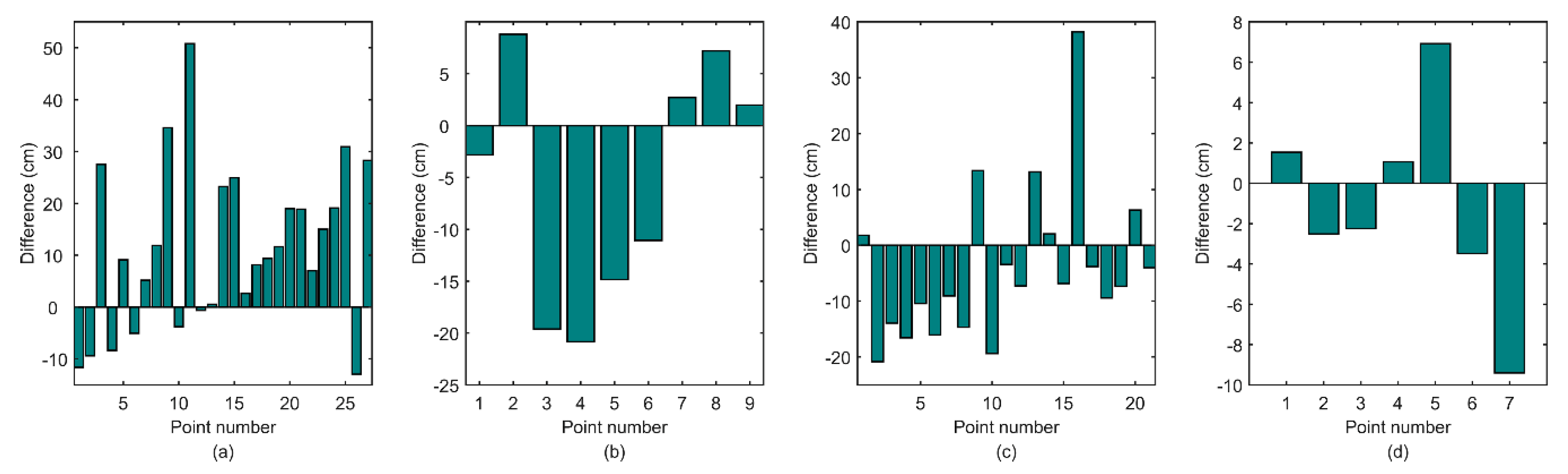
The statistics of comparison between these missions are presented in

Table 2. Statistics of Jason-series altimeter derived lake levels compared with the lake levels from ICESat and SARAL.

Difference 1	No. of Points	Min (cm)	Max (cm)	Mean (cm)	SD (cm)	RMS (cm)	CC
Jason-1* – ICESat	27	−13.0	50.8	11.3	15.7	19.1	0.97
Jason-2 – ICESat*	9	−20.8	8.8	−5.4	11.5	12.1	0.93
Jason-2* – SARAL	21	−20.9	38.2	−6.8	9.7	11.7	0.96
Jason-3 – SARAL*	7	−9.4	6.9	−1.2	4.7	4.8	0.94

¹ The asterisk indicates which mission data are used for interpolation.

and differences are plotted in Figure 7. It should be noted that interpolation is needed for comparison. In general, the data of Jason-series satellites are used for interpolation, because they have a larger number and a smaller temporal interval than ICESat or SARAL data. However, only one data point of ICESat is located in the period of Jason-2 and three points of SARAL are in the period of Jason-3. In the two cases, we used ICESat and SARAL data for interpolation.

According to the comparison, lake levels observed by Jason-1 are averagely higher than those by ICESat, with a mean difference of 11.3 cm. Whilst, Jason-2 observes lake level lower than ICESat. The SD and root mean square (RMS) errors of Jason-1 and Jason-2 with respect to ICESat are beyond 10 cm. The mean difference between Jason-2 and SARAL is $-6.8\pm 9.7$ cm, which is consistent with the difference between Jason-2 and ICESat. Relatively speaking, Jason-3 has a better agreement with SARAL. The maximum absolute difference is less than 10 cm between Jason-3 and SARAL, and the SD and RMS errors are about 5 cm. Mean lake levels from each overlapping pair of missions have a high correlation coefficient (CC) more than 0.9. By comparing subplots in Figure 7, there might be a systematic bias between lake levels observed by different altimeters. Figure 7a shows lake levels from Jason-1 are higher than those from ICESat. Other three subplots indicate Jason-2 and Jason-3 observed lower lake levels than ICESat and SARAL.

3.3. Bias Adjustment Between the T/P-Family Altimeters

The T/P-family satellites share the same ground track and have an overlap between two successive satellites for inter-satellite calibration. For example, the Jason-1 spacecraft launched in December 2001 was kept on the same ground track as T/P until August 15, 2002. Observations in the overlapped period can be used to analyze the lake level bias between two missions. Over the lake Ngangzi Co, 8 paired-sample observations were retrieved in the overlap between T/P and Jason-1. For Jason-2 and Jason-3, 18 paired-sample observations were found. No paired-sample observation could be available for Jason-1 and Jason-2, because the first valid data of Jason-2 over Ngangzi Co is from cycle 30 in April 2009, when the Jason-1 satellite had been moved to a new interleaved orbit in January 2009.

The differences between these paired-sample observations are shown in Figure 8. The maximum likelihood estimation is adopted to estimate the bias. In result, Jason-1 has a mean lake level bias of $2.5\pm 5.4$ cm with respect to T/P. The bias of Jason-3 with respect to Jason-2 is $-2.8\pm 3.5$ cm after removing an outlier. Since there is no overlapped observation between Jason-1 and Jason-2, we have to estimate the bias between them using their mean lake level differences with respect to ICESat in Table 2. Finally, all biases of Jason-1/2/3 with respect to T/P are determined and charted in

Table 3. Biases of Jason-1/2/3 with respect to T/P.

Satellite	Jason-1	Jason-2	Jason-3
Bias (cm)	2.5	−14.2	−17.0

.

3.4. Monthly Lake Level Time Series of Ngangzi Co

In order to generate monthly lake level time series, Gaussian filtering was applied to the observations after bias adjustment. Three kinds of filter window length (3, 6 and 12 months) were tested. Outlying observations were rejected which deviation from the filtered value was more than 3-sigma. The results are shown in Figure 9. The time series filtered with a 12-month window (magenta curve) is too smooth, with the intra-annual amplitudes dramatically attenuated. The results with a 3-month (blue curve) and a 6-month (green curve) window length are rather similar, keeping the energy very well. Relatively, the former has more small spikes than the latter. Therefore, we suggest using the 6-month-wide filter window.

According to the time series, the lake level of Ngangzi Co dropped with a negative trend of about -0.39 m/yr before 1998 and increased dramatically after 1998. The rising trend between 1998 and 2002 is even more than 1 m/yr. The change rate in 2003–2014 is 0.32 m/yr. The lake level declined by ~1 m in 2015 and raised again from 2006. The reversed trends have been observed by altimetry in previous studies [9,12]. For the first time, Hwang et al. [9] derived a lake level time series of Ngangzi Co using T/P GDR data. In total, Ngangzi’s lake level rose by ~8 m from 1998 to 2017, which partially contributed to the making of a new wetland [35]. Without retracking the waveforms, the resulting usable lake heights in Hwang et al. [9] were much less than those from this study and showed only annual variations. An improved result was presented using retracked T/P, Jason-2 and Jason-2 data in [12]. However, there is a big data gap between 1994 and 1995 in this updated result. Another problem is the large annual oscillations during the T/P mission which is difficult to explain. The method presented in this study acquired nearly continuous observations. Generated time series can reveal lake level variations with various periods. Figure 10 shows the continuous wavelet transform of the lake level time series using the bump wavelet [36]. It is demonstrated that not only annual and semi-annual variations but also interannual oscillations can be clearly observed in the time series.

4. Discussion

This study focused on the robust and accurate generation of lake level time series in Tibet. Although no in situ data could be used for validation in this case study, two independent datasets with higher accuracy from ICESat and SARAL were successfully applied to validate our results. In order to further demonstrate the advantage of our method, the comparison was performed between the presented results and other altimeter-derived time series products. There are several public global databases for inland water bodies, such as, the River and Lake database by the European Space Agency and De Montfort University (ESA-DMU) [37], The Hydroweb database by the Laboratoire d’Etudes en Géophysique et Océanographie Spatiales (LEGOS) [38], The Global Reservoir and Lake Monitor (G-REALM) by the Foreign Agricultural Service of the United States Department of Agriculture (USDA), and the Hydrological Time Series of Inland Waters (DAHITI) by the Deutsches Geodätisches Forschungsinstitut [30]. We searched these databases and only found results over the lake Ngangzi Co in G-REALM (alias Ang-tzu) and Hydroweb (alias Ngangze). G-REALM provided a time series from April 2009 to the present resulting from the Jason-2 and Jason-3 data. The time series from Hydroweb covered all the T/P-family missions from September 1992 to present.

Figure 11 shows the mean lake levels in this study in comparison to those from G-REALM and Hydroweb. All data are without smoothing and shifted from product datum to EGM96 geoid. Apparently, our method retrieved much more data from T/P and Jason-1. In the Jason-1 period, there are few data in Hydroweb and no data in G-REALM. Hence we only compared different time series in the Jason-2 and Jason-3 periods.

Table 4. Comparison of lake levels from different altimeter-derived products.

Product	Min (cm)	Max (cm)	Mean (cm)	SD (cm)	RMS (cm)	CC
G-REALM(Jason-2) - SARAL	−41.7	62.8	8.1	23.3	24.2	0.81
G-REALM(Jason-3) - SARAL	1.2	38.8	26.0	12.4	28.4	0.89
Hydroweb – SARAL	−219.5	−143.9	−191.2	15.6	191.8	0.94
G-REALM – this study	−281.2	20.7	2.4	24.7	24.8	0.88
G-REALM – this study 1	−6.5	20.7	7.8	5.0	9.2	0.99
Hydroweb – this study	−217.0	−185.5	−198.1	5.7	198.2	0.98

¹ The values in this row is estimated after removing anomalous data in G-REALM.

tabulates the statistic results. With respect to SARAL, the SDs and CCs for G-REALM and Hydroweb are inferior to our results (Table 2). For Jason-2 and Jason-3 data, the presented results in this study have a high agreement with G-REALM. However, many anomalous values can be found in G-REALM product from the zoom-in plot in Figure 11. After removing these anomalous values, the correlation between our results and G-REALM reaches to 0.99. Different biases can be found in Hydroweb product. A sharp drop of lake level happened in 2009, indicating that the bias between Jason-2 and Jason-3 was not properly adjusted in Hydroweb. With respect to our result and G-REALM, the lake level bias of Hydroweb is about −1.4 m during the T/P and Jason-1 missions before 2009 and about -2 m during the Jason-2 and Jason-3 missions. Two factors might explain the bias. T/P GDR data were used to construct the Hydroweb database, which is also the reason why fewer valid cycles were retrieved in Hydroweb. DTC in GDR contributes -1.06 m to the bias as shown in Section 2.2. The remaining bias might be caused by different waveform retracking algorithms used.

The case study of Ngangzi Co suggests that the accuracy of retrieved mean lake levels of the Tibetan lakes is much lower in summer than in winter. For example, the mean SD for T/P is 22.5 cm in July and August, whilst 17.3 cm in the winter season. Complex shapes of contaminated waveforms in summer degrade the accuracy of retracking algorithms. More sophisticated retracking method is still expected to improve the PSR of summer cycles. Waveform decontamination [39] presented for the coastal application may be potentially applicable to further refine altimeter measurements over the Tibetan lakes. It should be mentioned that the change in lake area was not considered in data processing. A static shoreline was used to extract altimeter data for all missions. This will cause some data on the shore may be extracted, especially when the lake level is low (e.g., in T/P period). The shrink of lake area will also make the lake level observation noisier. It can explain why the PSR value of T/P is so small. Modelling accurate time-varying shorelines is difficult and time-consuming work and need other data source, such as satellite imagery. Therefore, a procedure for outlier removal is often performed, instead of the consideration of dynamical lake boundary. Figure 5 has shown that the estimation of mean lake levels would be less affected by the lack of consideration of horizontal boundary, benefitted from the good performance of the outlier detection procedure proposed in this study.

Since it is difficult for early altimeters to maintain a lock on the rough terrain, Ngangzi Co is one of few Tibetan lakes which have been continuously monitored by satellite altimeters for more than 25 years. So far, we constructed a high-precision lake level time series with the most samples over Ngangzi Co using the T/P-family altimeters. As shown in Figure 10, our results allow monitoring lake level variations with various periods. The 25-year-long lake level time series is valuable for the hydrological and climatic studies. Combining with surface area changes detected by satellite imagery, it can be used to quantify the water volume balance of the lake basin. Previous studies [9,12] have shown that the lake level variation of Ngangzi Co is strongly correlative to ENSO. The long-term and uniform sampling time series generated in this study will greatly enhance the understanding of the relationship between the lake level variation and climate change.

Figure 12 shows surface temperature and precipitation in the lake basin, extracted from CPC global temperature and CMAP precipitation data provided by the NOAA/OAR/ESRL PSD, Boulder, Colorado, USA, from their Web site at https://www.esrl.noaa.gov/psd/. It suggests that the rise of lake level after 1998 can be primarily attributed to enhanced precipitation. The increased precipitation in this region since the late 1990s was also recorded by the nearby rain gauge [40]. According to field survey in this region, the lake level of Dagze Co, which is located on the northeast of Ngangzi Co with a distance of about 100 km, descended by 2 m in 1976–1999 and ascended by 8.2 m in 1999–2010 [40]. It is consistent with the altimeter-derived lake level change of Ngangzi Co in this study. A large drop in temperature between 1999 and 2000 can be observed in Figure 12. The descent of the surface temperature reduced evaporation, which would also contribute to the rise of lake level. Although the water flux shows good agreement with the seasonal variation of lake level, the quantitative relationship between each factor and water budget is not clear. This is a subject for future studies.

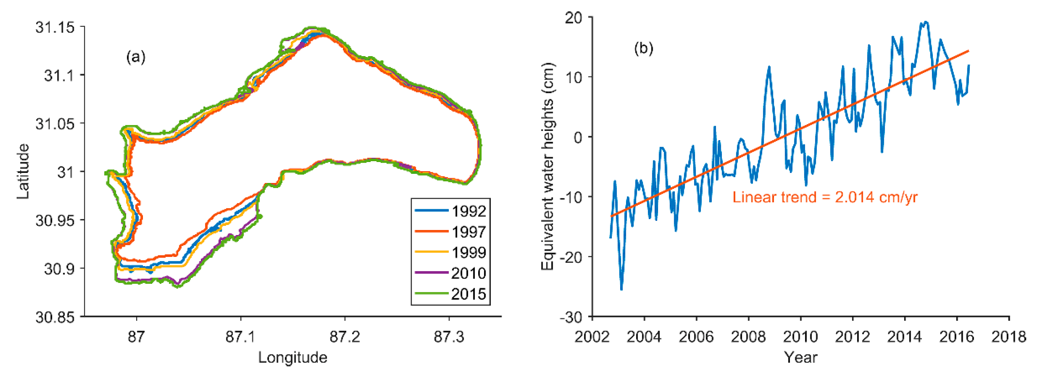
The altimeter-derived lake level change can also be confirmed by other independent satellite observations. Figure 13a illustrates the area change of Ngangzi Co from 1992 to 2015, downloaded from the Third Pole Environment (TPE) database (http://www.tpedatabase.cn/). The time series of lake area was constructed using Landsat images by Zhang et al. [41]. To avoid seasonal effects, images in October were mainly used to construct the time series. For the sake of clarity, we only plotted the shorelines in five years. However, it is enough to verify the change pattern of lake level. It can be seen that the lake area reached the minimum in 1997 and then continuously expanded, which is in accord with the lake level change observed by altimetry. Figure 13b is the equivalent water height (EWH) time series from August 2002 to June 2016, which is right at the center of Ngangzi Co. This EWH time series is derived using the CNES/GRGS RL04-v1 monthly gravity field solutions from the Gravity Recovery and Climate Experiment (GRACE) mission. It reflects the water storage around the lake has increased since 2002 and this trend is consistent with the trend of lake level change. However, it is unknown how the GRACE-detected water storage increase is related to the rise of lake levels. A detailed analysis combining multisource satellite observations and hydrological model is expected in the future.

5. Conclusions

Tibetan lakes are located in the high-altitude and rough-terrain region. Surface environment varies with seasons. Monitoring of lake level variation by altimetry is more difficult in Tibet than elsewhere. In this paper, a robust method was presented for generating lake level time series of Tibetan lakes using multi-altimeter data. In order to merge various altimeter data products issued in different ages, the consistency of geophysical corrections should be carefully checked. For the DTC, a large bias of about 1 m is found in T/P GDR data due to the high altitude with respect to the sea level. There is a DTC bias occurred from 2006 in Jason-1 and Envisat data. Hence, the DTCs should be updated using the same surface pressure model. Retracking correction is necessary for the accurate retrieval of lake level because the leading edges of waveforms over Tibetan lakes are seriously migrated from the theoretical tracking point. Three retrackers were evaluated in term of a presented parameter PSR, the ratio of the percentage of valid measurements to the SD of lake levels for each cycle. The ICE retracker relatively performs better than TR20 and TR50 in the case study. A two-step method was proposed for outlier removal, which has good performance without requiring any a priori information. Bias adjustment is also indispensable for the combination of altimeter data from multiple missions. The bias can be directly estimated using paired-sample measurements for two successive missions with an overlap, such as T/P and Jason-1, Jason-2 and Jason-3. However, there is a case without overlapping observations between Jason-1 and Jason-2. The problem is successfully solved by using ICESat data as the intermediary.

As a case study, a 25-year-long lake level time series, was generated for the lake Ngangzi Co using the T/P-family altimeter data. The mean lake levels can be retrieved with decimeter accuracy using the presented method. The mean SD is about 10 cm for Jason-1/2/3 and 17 cm for T/P. ICESat and SARAL have much better accuracy than T/P-family satellites, with a mean SD of 4.8 and 6.6 cm, respectively. Envisat also has data over the lake but nearly unusable. In spite of the relatively sparse sampling, ICESat and SARAL data can be used for validation. High correlation more than 0.9 can be observed between the mean lake levels from T/P-family satellites, ICESat and SARAL. Compared to the previous studies and available lake level databases, our result is the most robust time series for Ngangzi Co, with high accuracy and considerably continuous samples from October 1992 to December 2017. Jason-3 is still ongoing and its following mission Jason-CS will be launched in 2020 to extend the current lake level time series, providing un-interrupted lake level records for managing the wetland around Ngangzi Co. Such a long-term record can also be used to study the mechanism that has caused Ngangzi Co’s continuous lake level rise since 1998.

References

1. Wang, S.M.; Dou, H.S. Chinese Lakes Inventory; Science Press: Beijing, China, 1998; p. 403. [Google Scholar]
2. Ma, R.H.; Yang, G.S.; Duan, H.T.; Jiang, J.H.; Wang, S.M.; Feng, X.Z.; Li, A.N.; Kong, F.X.; Xue, B.; Wu, J.L.; et al. China’s lakes at present: Number, area and spatial distribution. Sci. China Earth Sci. 2011, 54, 283–289. [Google Scholar] [CrossRef]
3. Song, C.; Huang, B.; Ke, L.; Richard, K.S. Seasonal and abrupt changes in the water level of closed lakes on the Tibetan Plateau and implications for climate impacts. J. Hydrol. 2014, 514, 131–144. [Google Scholar] [CrossRef]
4. Song, C.; Huang, B.; Richards, K.; Ke, L.; Phan, V.H. Accelerated lake expansion on the Tibetan Plateau in the 2000s: Induced by glacial melting or other processes? Water Resour. Res. 2014, 50, 3170–3186. [Google Scholar] [CrossRef] [Green Version]
5. Phan, V.H.; Lindenbergh, R.; Menenti, M. ICESat derived elevation changes of Tibetan lakes between 2003 and 2009. Int. J. Appl. Earth Obs. Geoinf. 2012, 17, 12–22. [Google Scholar] [CrossRef]
6. Zhang, G.; Xie, H.; Kang, S.; Yi, D.; Ackley, S.F. Monitoring lake level changes on the Tibetan Plateau using ICESat altimetry data (2003–2009). Rem. Sens. Environ. 2011, 115, 1733–1742. [Google Scholar] [CrossRef]
7. Kleinherenbrink, M.; Lindenbergh, R.C.; Ditmar, P.G. Monitoring of lake level changes on the Tibetan Plateau and Tian Shan by retracking Cryosat SARIn waveforms. J. Hydrol. 2015, 521, 119–131. [Google Scholar] [CrossRef]
8. Jiang, L.; Neilsen, K.; Anderson, O.B.; Bauer-Gottwein, P. Monitoring recent lake level variations on the Tibetan Plateau using CryoSat-2 SARIn mode data. J. Hydrol. 2015, 544, 109–124. [Google Scholar] [CrossRef]
9. Hwang, C.; Peng, M.F.; Ning, J.; Luo, J.; Sui, C.H. Lake level variations in China from TOPEX/Poseidon altimetry: Data quality assessment and links to precipitation and ENSO. Geophys. J. Int. 2005, 161, 1–11. [Google Scholar] [CrossRef]
10. Lee, H.; Shum, C.K.; Tseng, K.H.; Guo, J.Y.; Kuo, C.Y. Present-Day Lake Level Variation from Envisat Altimetry over the Northeastern Qinghai-Tibetan Plateau: Links with Precipitation and Temperature. Terr. Atmos. Ocean. Sci. 2011, 22, 169–172. [Google Scholar] [CrossRef]
11. Gao, L.; Liao, J.; Shen, G. Monitoring lake-level changes in the Qinghai-Tibetan Plateau using radar altimeter data (2002–2012). J. Appl. Remote Sens. 2013, 7, 073470. [Google Scholar] [CrossRef]
12. Hwang, C.; Cheng, Y.S.; Han, J.; Kao, R.; Huang, C.Y.; Wei, S.H.; Wang, H. Multi-Decadal Monitoring of Lake Level Changes in the Qinghai-Tibet Plateau by the TOPEX/Poseidon-Family Altimeters: Climate Implication. Remote Sens. 2016, 8, 466. [Google Scholar] [CrossRef]
13. China Tibet Online. Available online: http://chinatibet.people.com.cn/6922554.html (accessed on 27 January 2019).
14. Okotto-Okotto, J.; Raburu, P.O.; Obiero, K.O.; Obwoyere, G.O.; Mironga, J.M.; Okotto, L.G.; Raburu, E.A. Spatio-temporal impacts of Lake Victoria water level recession on the fringing Nyando Wetland, Kenya. Wetlands 2018, 38, 1107–1119. [Google Scholar] [CrossRef]
15. Aviso User Handbook—Merged TOPEX/POSEIDON Products (GDR-Ms). Available online: https://www.aviso.altimetry.fr/fileadmin/documents/data/tools/hdbk_tp_gdrm.pdf (accessed on 9 January 2019).
16. OSTM/Jason-1 Products Handbook. Available online: http://www.aviso.altimetry.fr/fileadmin/documents/data/tools/hdbk_j1_gdr.pdf (accessed on 9 January 2019).
17. OSTM/Jason-2 Products Handbook. Available online: http://www.aviso.altimetry.fr/fileadmin/documents/data/tools/hdbk_j2.pdf (accessed on 9 January 2019).
18. OSTM/Jason-3 Products Handbook. Available online: http://www.aviso.altimetry.fr/fileadmin/documents/data/tools/hdbk_j3.pdf (accessed on 9 January 2019).
19. Crétaux, J.F.; Calmant, S.; Romanovski, V.; Shabunin, A.; Lyard, F.; Bergé-Nguyen, M.; Cazenave, A.; Hernandez, F.; Perosanz, F. An absolute calibration site for radar altimeters in the continental domain: Lake Issykkul in Central Asia. J. Geod. 2009, 83, 723–736. [Google Scholar] [CrossRef]
20. Vasiljevic, D.; Andersson, E.; Isaksen, L.; Garcia-Mendez, A. Surface pressure bias correction in data assimilation. ECMWF Newsl. 2006, 108, 20–27. [Google Scholar] [CrossRef]
21. Dee, D.P.; Uppala, S.M.; Simmons, A.J.; Berrisford, P.; Poli, P.; Kobayashi, S.; Andrae, U.; Balmaseda, M.A.; Balsamo, G.; Bauer, P.; et al. The ERA-Interim reanalysis: Configuration and performance of the data assimilation system. Q. J. R. Meteorol. Soc. 2011, 137, 553–597. [Google Scholar] [CrossRef]
22. Ho, C.M.; Wilson, B.D.; Mannucci, A.J.; Lindqwister, U.J.; Yuan, D.N. A comparative study of ionospheric total electron content measurements using global ionospheric maps of GPS, TOPEX radar, and the Bent model. Radio Sci. 1997, 32, 1499–1512. [Google Scholar] [CrossRef] [Green Version]
23. Brown, G. The average impulse response of a rough surface and its applications. IEEE Trans. Antennas Propag. 1977, 25, 67–74. [Google Scholar] [CrossRef]
24. Guo, J.Y.; Chang, X.T.; Gao, Y.G.; Sun, J.L.; Hwang, C. Lake level variations monitored with satellite altimetry waveform retracking. IEEE J. Sel. Top. Appl. Earth Obs. Remote Sens. 2009, 2, 80–86. [Google Scholar] [CrossRef]
25. Birkett, C.M.; Beckley, B. Investigating the performance of the Jason-2/OSTM radar altimeter over lakes and reservoirs. Mar. Geod. 2010, 331, 204–238. [Google Scholar] [CrossRef]
26. Uebbing, B.; Kusche, J.; Forootan, E. Waveform retracking for improving level estimations from TOPEX/Poseidon, Jason-1, and Jason-2 altimetry observations over African lakes. IEEE Trans. Geosci. Remote Sens. 2015, 53, 2211–2224. [Google Scholar] [CrossRef]
27. Yi, Y.C.; Kouraev, A.V.; Shum, C.K.; Vuglinsky, V.S.; Cretaux, J.F.; Calmant, S. The performance of altimeter waveform retrackers at lake Baikal. Terr. Atmos. Ocean. Sci. 2013, 24, 513–519. [Google Scholar] [CrossRef]
28. Tseng, K.H.; Shum, C.K.; Yi, Y.C.; Fok, H.S.; Kuo, C.Y.; Lee, H.; Cheng, X.; Wang, X.W. Envisat altimetry radar waveform retracking of quasi-specular echoes over the ice-covered Qinghai lake. Terr. Atmos. Ocean. Sci. 2013, 24, 615–627. [Google Scholar] [CrossRef]
29. Okeowo, M.A.; Lee, H.; Hossain, F.; Getirana, A. Automated generation of lakes and reservoirs water elevation changes from satellite radar altimetry. IEEE J. Sel. Top. Appl. Earth Obs. Remote Sens. 2017, 10, 3465–3481. [Google Scholar] [CrossRef]
30. Schwatke, C.; Dettmering, D.; Bosch, W.; Seitz, F. DAHITI—An innovative approach for estimating water level time series over inland waters using multi-mission satellite altimetry. Hydrol. Earth Syst. Sci. 2015, 19, 4345–4364. [Google Scholar] [CrossRef]
31. Vu, P.L.; Frappart, F.; Darrozes, J.; Marieu, V.; Blarel, F.; Ramillien, G.; Bonnefond, P.; Birol, F. Multi-Satellite Altimeter Validation along the French Atlantic Coast in the Southern Bay of Biscay from ERS-2 to SARAL. Remote Sens. 2018, 10, 93. [Google Scholar] [CrossRef]
32. Dettmering, D.; Schwatke, C.; Bosch, W. Global Calibration of SARAL/AltiKa Using Multi-Mission Sea Surface Height Crossovers. Mar. Geod. 2015, 38, 206–218. [Google Scholar] [CrossRef]
33. Guo, J.; Wang, J.; Hu, Z.; Hwang, C.; Chen, C.; Gao, Y. Temporal-spatial variations of sea level over China seas derived from altimeter data of TOPEX/Poseidon, Jason-1 and Jason-2 from 1993 to 2012. Chin. J. Geophys. 2015, 58, 3103–3120. [Google Scholar] [CrossRef]
34. Salcedo, C. Jason Orbit Acquisition and First Results of Station Keeping. In Proceedings of the International Symposium on Formation Flying, Toulouse, France, 29–31 October 2002. [Google Scholar]
35. Xue, Z.; Lyu, X.; Chen, Z.; Zhang, Z.; Jiang, M.; Zhang, K.; Lyu, Y. Spatial and temporal changes of wetlands on the Qinghai-Tibetan Plateau from the 1970s to 2010s. Chin. Geogr. Sci. 2018, 28, 935–945. [Google Scholar] [CrossRef]
36. MathWorks. Available online: https://in.mathworks.com/help/wavelet/ref/cwtft.html#buu64ch (accessed on 24 January 2019).
37. Berry, P.; Jasper, A.; Bracke, H. Retracking ERS-1 altimeter waveforms over land for topographic height determination: An expert system approach. In Proceedings of the Third ERS Symposium on Space at the service of our Environment, Florence, Italy, 14–21 March 1997; pp. 403–408. [Google Scholar]
38. Cretaux, J.-F.; Jelinski, W.; Calmant, S.; Kouraev, A.; Vuglinski, V.; Berge-Nguyen, M.; Gennero, M.-C.; Nino, F.; Abarca Del Rio, R.; Cazenave, A.; et al. SOLS: A lake database to monitor in the Near Real Time water level and storage variations from remote sensing data. Adv. Space Res. 2011, 47, 1497–1507. [Google Scholar] [CrossRef]
39. Huang, Z.; Wang, H.; Luo, Z.; Shum, C.K.; Tseng, K.-H.; Zhong, B. Improving Jason-2 sea surface heights within 10 km offshore by rertacking decontaminated waveforms. Remote Sens. 2017, 9, 1077. [Google Scholar] [CrossRef]
40. Lei, Y.; Yang, K.; Wang, B.; Sheng, Y.; Bird, B.W.; Zhang, G.; Tian, L. Response of inland lake dynamics over the Tibetan Plateau to climate change. Clim. Chang. 2014, 125, 281–290. [Google Scholar] [CrossRef]
41. Zhang, G.; Yao, T.; Piao, S.; Bolch, T.; Xie, H.; Chen, D.; Gao, Y.; O’Reilly, C.M.; Shum, C.K.; Yang, K.; et al. Extensive and drastically different alpine lake changes on Asia’s high plateaus during the past four decades. Geophys. Res. Lett. 2016, 44, 252–260. [Google Scholar] [CrossRef]
Figure 1. Study area and satellite ground tracks passing through the lake. The background is the topography extracted from the SRTM DEM.
Remotesensing 11 00558 g001
Figure 2. Atmosphere path delay corrections for the T/P-family missions. (a) Dry troposphere correction (DTC); (b) wet troposphere correction (WTC); (c) ionosphere correction (IC). A bias of -1.06 m is removed from the DTCs in the T/P GDR. The WTC for T/P is recomputed using the ECMWF model.
Remotesensing 11 00558 g002
Figure 3. Jason-2 altimeter waveforms in 2010 over Ngangzi Co. (a) Waveforms in the whole year; (b) A waveform in winter season from cycle 89; (c) a waveform in the summer season from cycle 71.
Remotesensing 11 00558 g003
Figure 4. The area graph for the comparison of three retrackers applied to the T/P-family missions: (a) T/P; (b) Jason-1; (c) Jason-2; (d) Jason-3. The y-axis PSR is the ratio of the percentage of valid measurements to the standard deviation of lake levels. The area is stacked showing the relative contribution of each retracker in a different color. TR50 and TR20 denote the 50% threshold and the 20% threshold retracker, respectively.
Remotesensing 11 00558 g004
Figure 5. Example of outlier detection in the case of Jason-1 observations over Ngangzi Co. Red dots are outliers detected in the 1st step. Green dots are outliers detected in the 2nd step. Blue dots are valid measurements and magenta triangles are mean lake levels for each cycle estimated after outlier removal. Standard deviations of lake levels are plotted as cyan stems.
Remotesensing 11 00558 g005
Figure 6. Mean lake levels derived from various satellites and histograms distribution of their SDs. (a) Mean lake levels; (b) TOPEX/Poseidon; (c) Jason-1; (d) Jason-2; (e) Jason-3. The red curve denotes the normal distribution fit.
Remotesensing 11 00558 g006
Figure 7. Differences of lake levels derived from the Jason-series altimeters with respect to the data from ICESat and SARAL. (a) Jason-1–ICESat; (b) Jason-2–ICESat; (c) Jason-2–SARAL; (d) Jason-3–SARAL.
Remotesensing 11 00558 g007
Figure 8. Difference between paired-sample observations of two successive missions. (a) Jason-1–T/P; (b) Jason-3–Jason-2. The green dashed line represents the mean value. The red dashed lines show a standard deviation from the mean. The red dot is an outlier removed before estimating the bias. The cycle numbers outside and in the parentheses are for the former and the following satellite, respectively.
Remotesensing 11 00558 g008
Figure 9. Lake level time series of Ngangzi Co after bias adjustment and monthly time series generated using Gaussian filters.
Remotesensing 11 00558 g009
Figure 10. Time-period analysis of the lake level time series of Ngangzi Co. (a) Continuous wavelet transform; (b) mean wavelet power spectrum.
Remotesensing 11 00558 g010
Figure 11. Lake level time series of Ngangzi Co from this study, G-REALM (only Jason-2 and Jason-3) and Hydroweb. The zoom-in plot shows large anomalous values in the time series from G-REALM.
Remotesensing 11 00558 g011
Figure 12. Monthly lake level variation of Ngangzi Co (right y-axis in blue), surface temperature (left y-axis in black) and precipitation rate (colormap). The red curve with circles shows the yearly mean temperature.
Remotesensing 11 00558 g012
Figure 13. (a) Lake area change of Ngangzi Co by satellite imagery [41] and (b) equivalent water height time series by GRACE.
Remotesensing 11 00558 g013