Remote Sensing for Optimal Estimation of Water Temperature Dynamics in Shallow Tidal Environments

Abstract

Given the increasing anthropogenic pressures on lagoons, estuaries, and lakes and considering the highly dynamic behavior of these systems, methods for the continuous and spatially distributed retrieval of water quality are becoming vital for their correct monitoring and management. Water temperature is certainly one of the most important drivers that influence the overall state of coastal systems. Traditionally, lake, estuarine, and lagoon temperatures are observed through point measurements carried out during field campaigns or through a network of sensors. However, sporadic measuring campaigns or probe networks rarely attain a density sufficient for process understanding, model development/validation, or integrated assessment. Here, we develop and apply an integrated approach for water temperature monitoring in a shallow lagoon which incorporates satellite and in-situ data into a mathematical model. Specifically, we use remote sensing information to constrain large-scale patterns of water temperature and high-frequency in situ observations to provide proper time constraints. A coupled hydrodynamic circulation-heat transport model is then used to propagate the state of the system forward in time between subsequent remote sensing observations. Exploiting the satellite data high spatial resolution and the in situ measurements high temporal resolution, the model may act a physical interpolator filling the gap intrinsically characterizing the two monitoring techniques.

1. Introduction

Lakes, estuaries, and lagoons around the world are degrading because of increasing human pressure, particularly due to water and sediments pollution and climate-change-related effects [1,2,3]. Among the coastal tidal systems, lagoons are probably the most threatened [4,5]. Lagoons occur along about 13 percent of the world’s shorelines [6] and play a fundamental role as morphological and biodiversity hotspots, providing valuable ecosystem services as for example refuge and nesting for a wide variety of wildlife, including mammals, marine birds, and migratory waterfowl. Lagoons play a primary role also in carbon cycle processes since they are characterized by rates of primary productivity comparable to that of rain forests, and consequently, they sequestrate a large amount of organic carbon in their typical morphological and biological entities such as marshes, mangroves, and seagrass meadows [7]. Beside their evident ecological importance, coastal lagoons are often the location of important urban centers, with relevant socioeconomic interests, leading to anthropogenic interference and rapid morphological and ecological modifications with concomitant losses of ecosystem goods and services. One emblematic and worldly famous example of the ecological, socioeconomical, and historical importance of world’s lagoons is the Venice Lagoon (Italy), which is the site selected for this research. Transformed over the long history of the Venetian Republic, the Venice Lagoon is now an example of the coexistence of the natural and the built environments, with evident tensions arising from sustainable and unsustainable uses of natural resources. As for other coastal systems, the monitoring of the dynamic processes that characterize the Venice Lagoon is of key importance for its correct management.

Water temperature is one of the main factors governing the biological processes occurring in aquatic ecosystems, such as open oceans and coastal waters as well as lakes and rivers. Temperature influences dissolved oxygen concentrations because affects its solubility, and as temperature increases, dissolved oxygen decreases [8,9]. However, the link between temperature and oxygen is far more complex since it is modulated by other abiotic factors as, for example, salinity, radiation, and wind action, as well as biotic factors. Moreover, a dependence on climatic conditions must also been accounted for. For warm climates, it has been recently shown that, in shallow water systems, photosynthetic organisms are stimulated by higher water temperature, producing more oxygen and supporting the metabolic demand of marine organisms [10]. In temperate climates, observations support the coexistence of two dynamics for shallow waters: a seasonal dynamics, characterized by high oxygen concentration during the colder part of the year and lower concentrations in the warmer, and a second diel dynamics, with maximum oxygen concentrations during the most irradiated hours of the day [11]. Temperature and oxygen dynamics are also affected by water circulation and stratification, with possible hypoxic events in areas with low water turnover [12,13,14]. The synergic action of water temperature, dissolved oxygen, and other environmental drivers as for example salinity, nutrients availability, and turbidity directly affect phytoplankton communities [15] and plant communities [16,17], with complex feedback mechanisms of vital importance for the state of lagoons and shallow coastal systems in general. As an example, we just mention the importance of a healthy population of seagrass or the proliferation of microalgae for the control of turbidity in shallow lagoons [16,18,19]. Furthermore, enclosed or semi-enclosed water bodies, such as lakes and lagoons, rapidly respond to variations in energy exchanges with the atmosphere, providing prompt signals related to climate change [1,20,21].

Traditionally, coastal and lagoon water properties and their dynamics are observed through point measurements carried out during field campaigns. Giving the increasing anthropogenic pressures on lagoons and coastal areas, in the last decades, methods for the continuous and spatially distributed monitoring of lagoon water quality (i.e., temperature or chlorophyll-a concentration) have become more common thanks to networks of sensors and probes. For example, besides the traditional gauges measuring water level (https://www.comune.venezia.it/it/content/centro-previsioni-e-segnalazioni-maree), the Venice Lagoon is continuously monitored through a network of 10 multi-parametric sensors since early 2000. Data collected from probes are often used to calibrate/validate hydrodynamic numerical models that describe the space/temporal evolution of a transported quantity. However, probe networks rarely attain a density sufficient for process understanding, model calibration and testing, or integrated assessment. This is arguably the most stringent limitation of state-of-the-art models of hydrodynamic flow and transport in shallow water environments, which are currently initialized and evaluated by making use of sparse and insufficient point observations. In this study, we show how the ideal observational tool, both for scientific and monitoring purposes, must integrate satellite data, in situ water quality data, and mathematical-physical models to provide a coherent space–time description of the dynamics of water quality and of the associated ecosystem properties.

Unfortunately, the majority of satellite sensors that collect thermal infrared data have too low a spatial resolution for applications to coastal systems characterized by high geomorphological diversity as lagoons and estuaries. For this application, we use Landsat ETM+ that provides thermal infrared data at 60 m spatial resolution. A set of two images collected seven days apart is selected from the archive (using USGS Earth Explorer website), data are calibrated with in situ measurements collected by a network of probes and used to produce the spatially distributed water temperatures. A numerical model of lagoon hydrodynamics and heat transport is then used as a physics-based interpolator to complete temperature data both in time and in space. Practically, the model is constrained using, as initial conditions (ICs), the temperatures retrieved from the first one of the two images and, as boundary conditions (BCs), other field measurements such as water levels at the seaward boundary of the domain and meteorological forcings acting at the atmosphere-water interface (e.g., wind speed and direction, solar radiation, air temperature, and humidity, etc.). The temperature dynamics is then simulated for seven days, and the temperatures retrieved using the second satellite image are then compared with the simulation results. Our results show how the combined use of point observations and of satellite images allow us to effectively constrain a model of temperature dynamics that, once calibrated, can overcome the intrinsic spatial and temporal limitations of those monitoring techniques providing a whole-system scale description of the process.

2. Materials and Methods

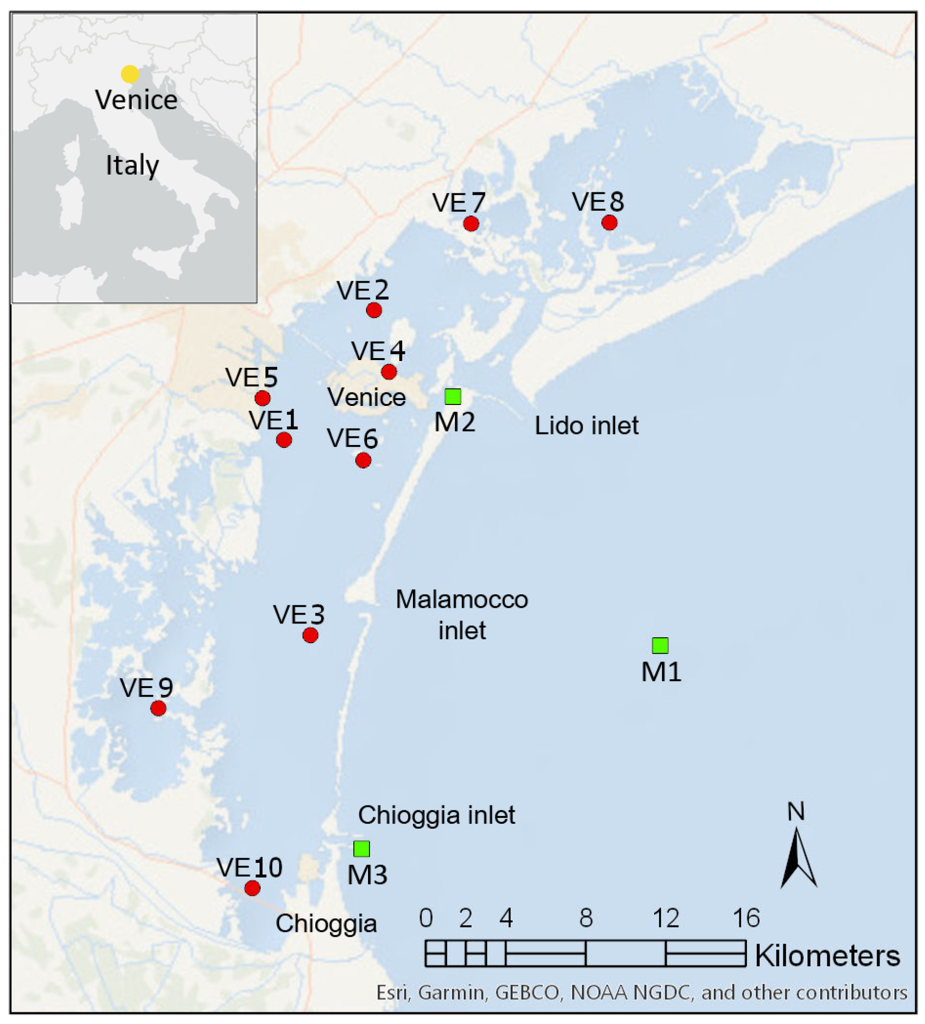
2.1. Study Site

The Venice Lagoon is the largest tidal basin in the Mediterranean Sea, covering an area of about 550 km${}^2$ (Figure 1). The mean depth characterizing the water basin is about 1.2 m, with a typical tidal range of 1.0 m and a main tidal period of 12 h. Beside its historical relevance, the Lagoon also represents a unique and dynamic ecosystem, hosting very peculiar habitats for multitude of animals and plant species.

Climate change and related sea level rise, subsidence of the bottom, and the anthropic pressure on the environments are threatening the Lagoon’s ecosystem, affecting its eco-bio-morphodynamic evolution [22]. The main environmental issues are the progressive reduction of the main morphological structures of the lagoonal environment, i.e., salt marshes and tidal flats, and the lagoon water quality. In the last 100 years, a reduction of about 40% of the salt marshes area and a 30% increase of the mean water depth has been observed, reinforcing the erosional trends by increasing the mean fetch and depth of the flows [23,24,25]. The modified hydrodynamics and the increased erosion and resuspension of sediments significantly affect also the water quality, spreading the pollutants accumulated in the Lagoon’s sediments. The main sources of pollution are the high nutrient load from water inflow, associated with agricultural activities and residential waste, and the industrial waste produced by the activities in the industrial estate of Marghera. The damages on the ecosystem caused by pollutants are worsened by the high residence time of water, which in the inner parts of the Lagoon can be of some tens of days [14].

To protect the city from increasingly stronger and more frequent flooding high tides [26,27], the MoSE (MOdulo Sperimentale Elettromeccanico) system is currently under construction. It is made up of a line of flap-gates built into each one of the three inlet canal beds that will emerge when needed to isolate the lagoon from the Adriatic Sea. Despite the importance of this infrastructure and the large amount of efforts put into its design, there is still a lack of knowledge about the impact of the MoSE system on the lagoon water quality. A reliable system to forecast the water quality dynamics during the closure of the gates has not been developed yet, especially considering a possible more frequent closure of the gates as sea level continues to rise [28].

With this study, we propose a multidisciplinary approach that integrates satellite data, in situ water quality data, and mathematical-physical models for studying and monitoring the Venice lagoon and that can be applied to other lagoons and coastal areas in order to couple biological, ecological, morphological and hydrodynamic processes and to understand the short- and long-term evolution of these environments and how we can preserve them.

2.2. Numerical Model

The numerical model consists of four modules: a hydrodynamic module, a wind-wave module, a Sediment Transport And Bed Evolution Module (STABEM) [29], and a temperature module. The coupling of the first two modules provides the Wind Wave Tidal Model (WWTM) [30,31].

Using a semi-implicit staggered finite element method based on Galerkin’s approach, the hydrodynamic module solves the two-dimensional shallow water equations, opportunely modified in order to deal with flooding and drying processes typical of very shallow and irregular domains, providing the evolution of water levels and depth-averaged velocities in space and in time. For a detailed description of the equations and of the numerical scheme adopted, see Defina [32] and D’Alpaos and Defina [33].

The wind wave module solves the wave action conservation equation following the parametrization proposed by Holthuijsen et al. [34], that uses the zero-order moment of the wave action spectrum in the frequency domain. The wind wave module exploits the water levels provided by the hydrodynamic module to compute the spatial and temporal distribution of the wave period using empirical correlation functions relating the mean peak wave period to local wind speed and water depth [31,35].

The WWTM reconstructs the spatial and temporal variability of the wind field over the computational domain when wind data from different measuring stations are available, using a suitable interpolation technique developed by Brocchini et al. [36].

The WWTM capability of reproducing the hydrodynamics and wind wave dynamics has been widely tested by comparing model’s results to field data collected not only in the Venice lagoon [31] but also in other lagoons such as lagoons located along the Virginia coast [37] and in the Cádiz Bay in Spain [38].

STABEM describes sediment resuspention and transport by simultaneously solving the advection diffusion equation and Exner’s equation, working on the same computational grid of WWTM. Following Soulsby [39], the model computes the total bottom shear stress as a nonlinear combination of wind-wave and tidal currents actions, leading to shear stresses values generally greater than the sum of the two contributions. The model adopts a stochastic approach similar to that proposed by Grass [40] to describe the sediment resuspension process, assuming the erosion rate to depend on the probability that the total bottom shear stress (${\tau }_b$) exceeds the critical shear stress (${\tau }_c$) for erosion, both treated as random variables characterized by a log-normal distribution. This stochastic approach significantly increases the capability of the model to describe the sediment resuspention process at near threshold conditions (i.e., values of ${\tau }_b\approx {\tau }_c$) for sediment entrainment, typical of periodical resuspention events occurring in shallow tidal basins [29,41].

STABEM accounts for the presence of both cohesive and non-cohesive sediments describing the bed composition as a mixture of two sizes sediment classes: non-cohesive sand and cohesive mud. The local mud content, which varies in time and space, determines the transition between non-cohesive and cohesive behavior of the mixture.

Temperature Module

The temperature module, developed to be coupled with WWTM and STABEM, is based on the solution of the heat advection and diffusion equation:

$$\frac{\partial T_{w}Y}{\partial t}+\nabla ·\left(\mathbf{q}{T}_w\right)-\nabla ·\left(Y\mathbf{D}·\nabla T_w\right)=\frac{H_{NET}}{{\rho }_{wat}{c}_{Pwat}}$$

(1)

where $T_w(°\mathrm{C})$ is the water temperature, assumed uniform within the water column based on the hypothesis of well-mixed conditions supported by field observation carried out in the Venice lagoon [42], $\mathbf{q}=(q_x,q_y)\left({\mathrm{m}}^3{\mathrm{s}}^{-1}{\mathrm{m}}^{-1}\right)$ is the flow rate per unit width, $Y\left[\mathrm{m}\right]$ is the equivalent water depth Defina (i.e., the volume of water per unit area as defined by [32]), $\mathbf{D}$ is the two dimensional diffusion tensor, $H_{NET}\left(\mathrm{W}{\mathrm{m}}^{-2}\right)$ is the net vertical energy flux, ${\rho }_{wat}\left(\mathrm{kg}{\mathrm{m}}^{-3}\right)]$, and $c_{Pwat}\left(\mathrm{J}{\mathrm{kg}}^{-1}\right)$ are the water density and the specific heat, respectively. Flow rates and water levels are provided by the hydrodynamic module, whereas the wind-wave module can provide information on the free surface roughness. Diffusivity is assumed equal to the eddy viscosity computed by the hydrodynamic model.

The suspended sediment concentration (SSC) is assumed to be in thermal equilibrium with water and unable to affect the water thermal properties.

$H_{NET}$ consists of the sum of the following energy fluxes at the atmosphere–water interface (AWI): (i) short-wave radiation $H_{sho}$, (ii) long-wave radiation $H_{lon}$, (iii) sensible heat flux $H_{sen}$, and (iv) latent heat flux $H_{lat}$. The net energy flux should also account for the conduction heat exchange at the soil–water interface (SWI), of which the calculation requires also the modeling of the bed sediment temperature. However, recent studies proved that, given the quite turbid conditions typically characterizing the Venice lagoon, the energy flux at the SWI is negligible when modeling the water temperature dynamics at the daily timescale [42]. Therefore, this contribution to the net energy flux affecting the water column temperature dynamics has been neglected in the present study.

The short-wave radiation flux $H_{sho}$ corresponds to the solar irradiance not reflected by the water surface and partially absorbed by the water column according to Beer’s law integrated over the water column [43]:

$$H_{sho}=(1-a)R_{sun}\left[1-exp\left(-\eta Y\right)\right]$$

(2)

where a is the water surface albedo, $R_{sun}\left(\mathrm{W}{\mathrm{m}}^{-2}\right)$ is the solar radiation measured at the surface, and $\eta \left({\mathrm{m}}^{-1}\right)$ is the extinction coefficient representing the irradiance absorption per unit depth. The coefficient $\eta$ should be time variant as a function of the water column turbidity (i.e., $\eta$ increases with turbidity); however, for the sake of simplicity, $\eta$ is assumed to be constant in the present study as we selected for our analysis a period characterized by the absence of storms and related intense resuspension events in order to avoid cloud coverage undermining the analysis of the available satellite images. Furthermore, we recently demonstrated (i) that, on average, the solar radiation absorption by the water column in the Venice lagoon is better described by values of $\eta >4$ [42], meaning that the water column absorbs most of the solar radiation and (ii) that most of the energy not absorbed by the water column under clear water conditions (described by small values of $\eta$) is returned to the water column via conduction at the SWI and that, then, the assumption of high values of $\eta$ to model the water column temperature dynamics provides the best results when the conductive heat exchange at the SWI is neglected [19].

The long-wave radiation flux $H_{lon}$ is the difference between the infrared radiation emitted by the atmosphere and the infrared radiation emitted by the water body. Following Bignami et al. [44], $H_{lon}$ is computed as follows:

$$H_{lon}=\sigma T_{air}^4(0.653+0.00535·e_{Vair})(1-0.1762·N^2)-ϵ\sigma T_w^4$$

(3)

where $\sigma \left(\mathrm{W}{\mathrm{m}}^{-2}{\mathrm{K}}^{-4}\right)$ is the Stefan–Boltzman constant, $T_{air}\left(\mathrm{K}\right)$ is the air temperature, $e_{Vair}\left(mbar\right)$ is the vapor pressure at $T_{air}$, N is the fraction of sky covered by clouds, and $ϵ$ is the water emissivity. The first term on the right-hand side is the long-wave radiation emitted by the atmosphere and fully absorbed by the water column, while the second term is the long-wave radiation emitted by the water body according to its temperature.

The sensible heat flux, $H_{sen}$, and the latent heat flux, $H_{lat}$, represent the energy transfer at the AWI due to conduction/convection and to evaporation, respectively. The temperature module estimates $H_{sen}$ and $H_{lat}$ using a “bulk” algorithm, a common approach in numerical models based upon the Monin–Obukhov Similarity Theory:

$$\begin{array}{c}{H}_{sen}={\rho }_{air}{c}_{Pair}{C}_{sen}{V}_{wind}(T_w-T_{air})\end{array}$$

(4)

$$\begin{array}{c}{H}_{lat}={\rho }_{air}{L}_v{C}_{lat}{V}_{wind}(q_S-q_{air})\end{array}$$

(5)

where ${\rho }_{air}\left(\mathrm{kg}{\mathrm{m}}^{-3}\right)$ and $c_{Pair}\left(\mathrm{J}{\mathrm{kg}}^{-1}\right)$ are air density and specific heat respectively, $L_v\left(\mathrm{J}{\mathrm{kg}}^{-1}\right)$ is the latent heat of vaporization, and $q_S$ and $q_{air}$ are the specific humidity at the sea surface and at the measuring height respectively. The transfer coefficients are estimated as follows:

$$\begin{array}{c}{C}_{sen}=k^2{\left(ln\frac{z_V}{z_0}-{\mathsf{\Psi }}_V\left(\frac{z_V}{L}\right)\right)}^{-1}{\left(ln\frac{z_T}{z_{0T}}-{\mathsf{\Psi }}_T\left(\frac{z_T}{L}\right)\right)}^{-1}\end{array}$$

(6)

$$\begin{array}{c}{C}_{lat}=k^2{\left(ln\frac{z_V}{z_0}-{\mathsf{\Psi }}_V\left(\frac{z_V}{L}\right)\right)}^{-1}{\left(ln\frac{z_Q}{z_{0Q}}-{\mathsf{\Psi }}_Q\left(\frac{z_Q}{L}\right)\right)}^{-1}\end{array}$$

(7)

where k is the Von Kármán constant (assumed equal to 0.4); $z_V$, $z_T$, and $z_Q$ $\left(\mathrm{m}\right)$ are the measuring heights while $z_0$, $z_{0T}$, and $z_{0Q}$ $\left(\mathrm{m}\right)$ are parameters called roughness lengths that characterize the neutral transfer properties for wind, temperaturem and humidity, respectively; and $L\left(\mathrm{m}\right)$ is the Obukhov length. ${\mathsf{\Psi }}_V$, ${\mathsf{\Psi }}_T$, and ${\mathsf{\Psi }}_V$ are empirical functions describing the stability dependence of the mean profile [45,46,47]. Using the Monin–Obukhov Similarity Theory, the roughness lengths, the Obukhov length, and the energy fluxes are computed iteratively [48,49]; in particular, in our code, we use the algorithm COARE 3.0 [50] to estimate the sensible and latent heat fluxes. The algorithm has already been tested to estimate the energy fluxes in a lagoon located along the Mediterranean french coast, providing satisfactory results [51].

The temperature module computes the roughness length $z_0$ as follows [48]:

$$z_0=\alpha \frac{u_{*}}{g}+0.11\frac{\nu }{u_{*}}$$

(8)

where $\alpha$ is the Charnock parameter, $u_{*}$ is the friction velocity over the water surface, and $\nu$ is the kinematic viscosity of water. According with Yelland and Taylor [52], $\alpha$ increases monotonically for $6<V_{wind}<26\mathrm{m}{\mathrm{s}}^{-1}$; the algorithm COARE accounts for this behavior linearly increasing $\alpha$ from $0.011$ at $V_{wind}=10\mathrm{m}{\mathrm{s}}^{-1}$ to $0.018$ at $V_{wind}=18\mathrm{m}{\mathrm{s}}^{-1}$ [50].

2.3. In Situ Measuring Stations

The meteorological data necessary to compute energy fluxes at the AWI were provided by the mareographic network of the Venice lagoon and the northern Adriatic coast, managed by the Institute for Environmental Protection and Research (Istituto Superiore per la Protezione e la Ricerca Ambientale—ISPRA). The real time gauge network collects water level; however, several measuring stations are equipped with additional sensors for measuring meteorological variables.

In detail, the data we use to constrain our temperature model at the AWI are air temperature $T_{air}$ $(°\mathrm{C})$, solar radiation $R_{sun}$ $\left(\mathrm{W}{\mathrm{m}}^{-2}\right)$, and relative humidity $H_{rel}$ $(\%)$ measured at the Lido Meteo station; wind speed $V_{wind}$ $\left(\mathrm{m}{\mathrm{s}}^{-1}\right)$ and direction $D_{wind}$ $\left(GN\right)$ measured at the Chioggia Diga Sud station; and atmospheric pressure $p_{atm}$ (mbar) measured at the Piattaforma CNR station. Meteorological variables are assumed spatially uniform over the entire lagoon.

The fraction of covered sky, N, which is a proxy for cloudiness, is another parameter affecting the energy fluxes at the AWI and in particular $H_{lon}$. Since cloudiness data are typically unavailable, in our simulation, we considered a constant cloudiness, corresponding to a clear sky condition ($N=0$), in line with the abovementioned choice of analyzing a period mostly characterized by clear weather.

Sea water temperature ($T_{sea}$) and water levels measured at the Piattaforma CNR station are then used as boundary conditions (BCs) for the model and imposed at the seaward boundary of the computational domain.

Water temperature ($T_w$) time series provided by the network of 10 multi-parametric probes, managed by Provveditorato per le Opere Pubbliche del Triveneto, are used to evaluate the capability of the model to describe the local temperature dynamics.

The locations of all the in situ measuring stations providing the data described above are shown in Figure 1. Figure 2 summarizes the time series used as BC for the numerical model.

2.4. Temperature Spatial Distribution from Satellite Images

Satellite data are selected based on four main requirements: (1) high spatial resolution (i.e., in the order of $50/100\mathrm{m}$) of the thermal infrared bands; (2) very good weather conditions in order to limit the interference of clouds and haze; (3) availability of at least one couple of images collected less than 10 days apart; and (4) satellite data overlap with available time series of field data (i.e., tidal levels, water temperature collected with probes, wind speed and direction, solar radiation, and relative humidity). The first image provides the water temperature spatial distribution at the beginning of the numerical simulation, while the subsequent images are used for comparison with numerical results. The requirement of very good weather conditions is strictly necessary for the first image in order to correctly initialize the system, while, in general, a partial lack of data due to clouds cover can be accepted in images used for model validation. Nonetheless, in the present analysis, we required very good weather conditions also for the second image in order to fully exploit information provided by satellite data and to perform the most complete and robust comparison with the computed spatial distribution of the water temperature at the end of the simulated period. We underline that a clear-sky image used for validating the simulation results allows a comprehensive evaluation of all the differences that may occur between the image and the simulation outcomes at the basin scale, providing information on areas that are not monitored by the probes network.

Several images freely available in the USGS Earth Explorer database were considered (e.g., from different Landsat missions and ASTER). Two ETM+ cloud-free images were found to be suitable for our analysis, one collected on 2 May 2008 and the second collected on 9 May 2008.

The ETM+ (Enhanced Thematic Mapper Plus), launched on 15 April 1999 on board of the Landsat 7 payload, includes one single-band sampling part of the thermal infrared (TIR) portion of the electromagnetic spectrum, spanning the 10.40–12.50 $\mathsf{\mu }$m wavelength range, with a spatial resolution at the ground of only $60\mathrm{m}$. Four years after the launch, on 31 May 2003, the Scan Line Corrector (SLC) in the ETM+ instrument failed. Therefore, since that date, the sensor was no longer able to scan the ground correctly, resulting in some areas that are not detected during the acquisition. It is estimated that, in one ETM+ scene, about 22% of the data is missing.

The interference of the atmosphere on satellite TIR data is mainly due to the absorption of the radiation by water vapor, $C{O}_2$, and $O_3$, while the scattering effect is negligible because of the long TIR wavelengths. Taking into account the atmospheric transmittance ${\tau }_{\lambda }$ for band $\lambda$, the spectral radiance measured at sensor, $L_{\lambda }^{at-sensor}$, is calculated as follows [53,54]:

$$L_{\lambda }^{at-sensor}=\left[{ϵ}_{\lambda }{B}_{\lambda }\left(T\right)+\left(1-{ϵ}_{\lambda }\right)L_{\lambda }^{\downarrow }\right]{\tau }_{\lambda }+L_{\lambda }^{\uparrow }$$

(9)

where $B_{\lambda }$ is the spectral radiance of a black-body, T is the true surface temperature, ${ϵ}_{\lambda }$ is the emissivity of the considered target, $L_{\lambda }^{\downarrow }$ is the down-welling atmospheric radiance and the $L_{\lambda }^{\uparrow }$ is the radiance emitted toward the sensor (which is, in case of ETM+, nadir looking).

Inverting Equation (9) in order to obtain the spectral radiance and integrating over the thermal bandpass, we obtain the following:

$$B\left(T\right)=\frac{L^{at-sensor}-L^{\uparrow }}{ϵ\tau }-\frac{1-ϵ}{ϵ}{L}^{\downarrow }$$

(10)

which, in order to calculate the temperature in Celsius, can be directly used in

$$T=\frac{k_2}{ln\left(\frac{k_1}{B\left(T\right)}+1\right)}-273.15$$

(11)

with, for ETM+, $k_1=666.09$ $\left(\mathrm{W}{\mathrm{m}}^{-2}{\mathrm{sr}}^{-1}\mathsf{\mu }{\mathrm{m}}^{-1}\right)$ and $k_2=1282.71$ $\left(\mathrm{K}\right)$.

$L^{\downarrow }$, $L^{\uparrow }$, and $\tau$ have been calculated using the Atmospheric Correction Parameter Calculator tool made available online by NASA (https://atmcorr.gsfc.nasa.gov/; Barsi et al. [55]) that uses the radiative transfer code MODTRAN. The expected accuracy of the correction is within ±2–3 $\left(\mathrm{K}\right)$ [55]. As for the emissivity, we used the constant value $ϵ=0.98$ for the entire water body of the lagoon. Pixels that do not belong to the water body were masked according to the computational domain of the hydrodynamic model. Moreover, we created a $120\mathrm{m}$ wide buffer along the coast line in order to mask also the pixels that fall at the water/land edge (with mixed signal) that may present unrealistic water temperature values. Finally, in order to fill the gaps in the ETM+ data due to the malfunctioning of the SLC, we applied a Multilevel B-Spline Approximation [56].

All the symbols used in the present study are summarized in

Table 1. List of symbols used for variables and constants: formulas are not explicitly discussed in Section 2.

Symbol	Description	Value	Unit
a	water surface albedo	$0.04$
$c_{Pair}$	air specific heat	1005	$\left[\mathrm{J}{\mathrm{kg}}^{-1}\right]$
$c_{Pwat}$	water specific heat	4186	$\left[\mathrm{J}{\mathrm{kg}}^{-1}\right]$
$C_{lat}$	bulk transfer coefficient
$C_{sen}$	bulk transfer coefficient
$e_0$	saturation vapor	$6.11$	[mbar]
	pressure at 0.0 °C
$\mathbf{D}$	two dimensional diffusion tensor
$e_V$	vapor pressure		[mbar]
$e_{VS}$	saturation vapor pressure		[mbar]
$H_{lat}$	latent heat flux		$\left[\mathrm{W}{\mathrm{m}}^{-2}\right]$
$H_{lon}$	net long wave heat flux		$\left[\mathrm{W}{\mathrm{m}}^{-2}\right]$
$H_{NET}$	net heat flux		$\left[\mathrm{W}{\mathrm{m}}^{-2}\right]$
$H_{sen}$	sensible heat flux		$\left[\mathrm{W}{\mathrm{m}}^{-2}\right]$
$H_{sho}$	short wave heat flux		$\left[\mathrm{W}{\mathrm{m}}^{-2}\right]$
k	Prandtl constant	$0.4$
L	Obukhov length		[m]
$L_v$	latent heat of evaporation		$\left[\mathrm{J}{\mathrm{kg}}^{-1}\right]$
N	fraction of covered sky
$\mathbf{q}=(q_x,q_y)$	flow rate per unit width		$\left[{\mathrm{m}}^3{\mathrm{s}}^{-1}{\mathrm{m}}^{-1}\right]$
$q_{air}$	air specific humidity
$q_S$	saturated air specific
	humidity at $T_w$
$R_{sun}$	incident solar radiation		$\left[\mathrm{W}{\mathrm{m}}^{-2}\right]$
t	time		[s]
$T_0$	temperature in K	$273.15$	[K]
	corresponding to 0 °C
$T_{air}$	air temperature		[C]
$T_w$	water temperature		[C]
$H_{rel}$	relative humidity		(%)
$V_{wind}$	wind speed		$\left[\mathrm{m}{\mathrm{s}}^{-1}\right]$
Y	equivalent water depth		[m]
$u_{*}$	friction velocity		$\left[\mathrm{m}{\mathrm{s}}^{-1}\right]$
$z_0$	roughness length for $V_{wind}$		[m]
$z_{0Q}$	roughness length for $H_{rel}$		[m]
$z_{0T}$	roughness length for $T_{air}$		[m]
$z_Q$	measuring height for $H_{rel}$		[m]
$z_T$	measuring height for $T_{air}$		[m]
$z_V$	measuring height for $V_{wind}$		[m]
$\alpha$	Charnock parameter
$ϵ$	water surface emissivity	$0.98$
$\lambda$	extinction coefficient		$\left[{\mathrm{m}}^{-1}\right]$
${\rho }_{air}$	air density	$1.225$	$\left[\mathrm{kg}{\mathrm{m}}^{-3}\right]$
${\rho }_{wat}$	water density	1027	$\left[\mathrm{kg}{\mathrm{m}}^{-3}\right]$
$\sigma$	Stefan Boltzman constant	$5.5576·{10}^{-8}$	$\left[\mathrm{W}{\mathrm{m}}^{-2}{K}^{-4}\right]$
$L_{\lambda }^{at-sensor}$	measured spectral radiance		$\left[\mathrm{W}{\mathrm{sr}}^{-1}{\mathrm{m}}^{-3}\right]$
${ϵ}_{\lambda }$	emissivity
$B_{\lambda }$	spectral radiance of a black body		$\left[\mathrm{W}{\mathrm{sr}}^{-1}{\mathrm{m}}^{-3}\right]$
${\tau }_{\lambda }$	atmospheric transmittance
$L_{\lambda }^{\downarrow }$	down-welling atmospheric radiance		$\left[\mathrm{W}{\mathrm{sr}}^{-1}{\mathrm{m}}^{-3}\right]$
$L_{\lambda }^{\uparrow }$	radiance emitted toward the sensor		$\left[\mathrm{W}{\mathrm{sr}}^{-1}{\mathrm{m}}^{-3}\right]$
$L_v=2.501·{10}^6-2370·\left(T_{air}\right)$
$e_{VS}=e_0·exp\left(17.502·T/(T+240.97)\right)·\left(1.0007+3.46·{10}^{-6}·p_{atm}\right)$
$e_V=e_{VS}·H_{rel}/100$
$q=0.622·e_v{\left(p_{atm}-0.378·e_v\right)}^{-1}$

.

3. Results

3.1. Temperature Spatial Distribution from Remote Sensing and Probes

The comparison between the water temperature retrieved from satellite data and recorded using the network of probes imply some considerations. As already specified, ETM+ collects TIR data at $60\mathrm{m}$ spatial resolution; hence, the first assumption we made is that the data collected by any single probe are representative of an area of at least $60\mathrm{m}\times 60\mathrm{m}$ and, hence, that we can directly compare it to the temperature value of the pixel containing the station. We further consider that the temperature recorded by each probe is representative of the entire water column, thus assuming well-mixed conditions within the water column. Such an assumption is supported by water temperature profiles that we recently collected in the Venice lagoon [42] and by other water temperature measurements collected in previous studies [57]. Another important consideration is that satellite data represent the “skin temperature”, i.e., the temperature of the water surface, rather than the bulk water temperature. The difference between skin and bulk temperature has been estimated for ocean [58] and lake [59] conditions and has been found to be less than $\pm 1\mathrm{K}$.

Figure 3a,b show the differences between the temperatures measured at each station and those retrieved from remote sensing and highlight how the difference among the two datasets is site dependent, probably because of local environmental conditions. As for the skin/bulk temperature difference, for example, it may vary due to different wind speeds at different locations. We must also consider that a single set of parameters ($L_{\lambda }^{\downarrow }$, $L_{\lambda }^{\uparrow }$, and ${\tau }_{lambda}$) computed using the radiative transfer code was used for the entire lagoon, neglecting the spatial variability of the atmospheric conditions that may affect the retrievals at different locations. Finally, the above assumptions about the difference in scale between measurements performed by probes and retrievals coming from satellite data may also depend on local conditions. As an example, we notice that the temperatures retrieved from ETM+ data for probe 4 are higher than those recorded by the probe for both the 2nd and the 9th of May 2008 and we speculate that this is due to the proximity of this probe to the city of Venice, with possible presence of local urban water discharges. In general, we consider as outliers (i.e., values that are more than three scaled median absolute deviations away from the median) the measurements coming from probes 1, 4, 7, and 10 for May the 2nd (Figure 3b), and the measurements coming from probes 4 and 9 for May the 9th (Figure 3e). Figure 3b,e show that the standard deviations greatly improve once the outliers are removed from the dataset.

Based on the mean standard deviation calculated for each image, we apply a correction to the temperatures retrieved from satellite data. Figure 3c,f shows a comparison between the temperatures measured by the probes and temperatures retrieved from satellite data after the correction. The temperature difference has been sensibly reduced, greatly improving the correlation between the temperature recorded by probes and those retrieved from satellite data.

3.2. Model Results

With the aim of developing and testing an integrated approach for water temperature monitoring, we perform a one-week-long model simulation for temperature dynamics in the Venice Lagoon using spatially distributed data from the two selected satellite images (see Section 2.4) and high-frequency point observations (see Section 2.3).

Data from the first satellite image are used to initialize the water temperature spatial distribution within the computational domain; accordingly, the simulation starts at the acquisition time of the first collected image (2 May 2008, 10:30) and ends at the acquisition time of the second image (9 May 2008, 10:30). We compare model results with time series of water temperature collected by the monitoring station along the simulated week and the spatial distribution of the water temperature, at the end of the simulation, with the water temperature map retrieved processing the second satellite image.

The meteorological variables driving the energy fluxes dynamics are assumed spatially uniform over the entire lagoon; hence, the spatial variability of the computed energy fluxes, due only to $T_w$ and Y, is limited. For this reason, in Figure 4, we show only the energy fluxes at the AWI computed by the model at the VE-2 station as they can be considered representative of the entire lagoon. In particular, Figure 4a shows the energy fluxes dynamics while Figure 4b shows the relative contribution of each flux $H_i$ to the total vertical energy exchanged: ${\sum }_i\left|H_i\right|$. The energy flux and its contribution are positive when directed toward the water column, i.e., when the flux is warming the water.

The comparison between in situ observations and computed water temperature at Station VE-2 and VE-3 is shown in Figure 5 and Figure 6, respectively. The two measuring stations are selected among the ten available in situ ones since they are representative of two peculiar locations within the water basin: the VE-2 station is located in the inner part of the Lagoon and quite close to the divide between two subbasins (namely the Lido Treporti and the Lido San Nicolò subbasins, i.e., the two main branches of the Lido inlet), where the advective transport is reasonably low, whereas the VE-3 Station is quite close to the Malamocco inlet, directly exposed to ebb and flood tidal currents (the location of the measuring stations are shown in Figure 1). Figure 5a and Figure 6a show the observed and computed time evolution of $T_w$ and of the cumulative vertical energy exchange, $E\left(t\right)={\int }_0^t{H}_{NET}dt$ $\left(\mathrm{J}{\mathrm{m}}^{-2}\right)$ provided to the water column. In both cases, model results are in good agreement with the local temperature data, highlighting the capability of the model to correctly describe the water temperature dynamics. To highlight the main factors that drive temperature fluctuations within the lagoon, Figure 5b and Figure 6b show the difference between water temperature computed at the measuring station and water temperature imposed as BC at the sea boundary of the numerical domain as well as the water level at the measuring station (see the Discussion section for an in-depth assessment of the matter).

The effectiveness of the model in reproducing the water temperature dynamics is also confirmed by the comparison of the spatially distributed temperature field at the end of a 7-day-long simulation, as shown in Figure 7. The difference between modeled and observed water temperature, $\mathsf{\Delta }{T}_w=T_w^{Mod}-T_w^{Obs}$, computed on each element of the computational grid (see Figure 7c), is lower than $\pm 1°\mathrm{C}$ on about the $65\%$ of the entire wet surface of the lagoon, and only on the $17\%$ of the wet surface, $\mathsf{\Delta }{T}_w$ exceeds values of $\pm 2°\mathrm{C}$. The mean value of $\left|\mathsf{\Delta }{T}_w\right|$, weighted on the area of the elements, is $1.27\pm 2.15°\mathrm{C}$.

4. Discussion

As described in the above sections, thermal infrared data detected by Landsat ETM+ satellite are shown to be able to provide meaningful and detailed representations of the spatial distribution of skin water temperature for complex coastal environments as the lagoon of Venice. The $60\mathrm{m}$ resolution of such temperature maps allows capturing significant spatial patterns of water temperature that characterize different parts of the lagoon (e.g., the area in front of the industrial estate of Marghera affected by the thermal plums due to production activities as well as the areas in front of the inlets affected by tidal currents). The skin temperature obtained from satellite data is a reliable proxy for bulk temperature, particularly for shallow and well-mixed water bodies; we have shown that simple corrections based on available in situ observations can greatly increase the agreement between skin and bulk temperature.

Considering that water temperature fields from remotely sensed data are rather infrequent (weekly or less frequent), a two-dimensional numerical model solving for hydro- and water temperature dynamics has been developed and used to describe the continuous-time spatial distribution of the water temperature within the entire Venice lagoon.

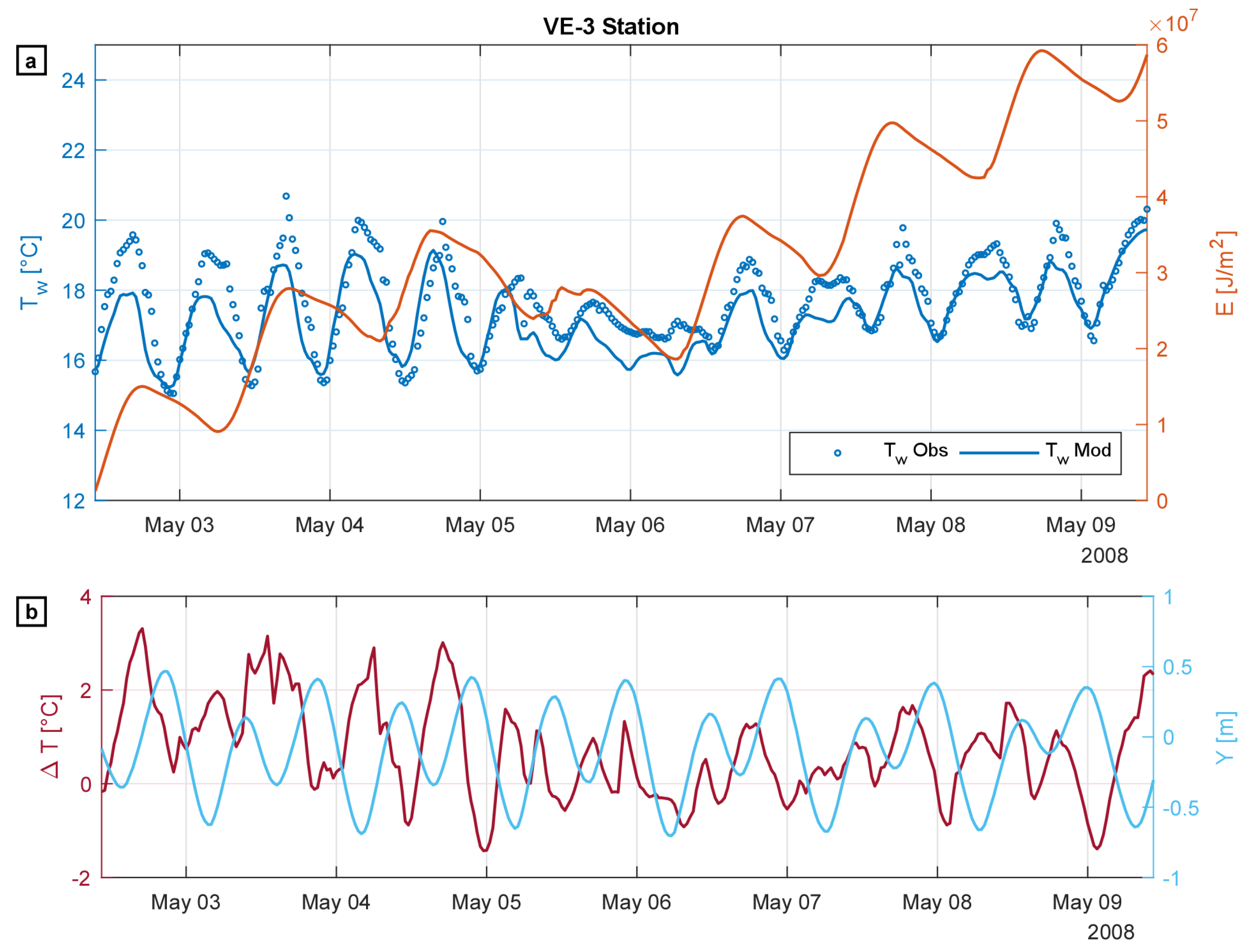
Model results have been, at first, compared with time series of water temperature recorded at 10 in situ measuring stations, displaying a quite good agreement with data. The numerical model correctly describes the temperature dynamics both in the inner areas of the water basin (Figure 5), which are mildly affected by heat transport associated with tidal currents, and close to the sea inlets (Figure 6), where advective transport plays a crucial role. It clearly emerges that, in the inner lagoon areas, the water temperature $T_w$ and the cumulative energy flux E at the AWI show the same diurnal modulation; here, advective heat fluxes induced by 6-h period tidal currents are negligible and the water temperature is mostly driven by the net energy flux at the AWI that follows the day and night cycle. Close to the inlets, while the cumulative energy flux E still displays a diurnal modulation, the water temperature $T_w$ is characterized by a semi-diurnal modulation clearly related with the tidal oscillation. Regardless of E, $T_w$ decreases during the flood phase because of the colder water entering the lagoon from the sea (through the Malamocco inlet in the case of the VE-3 station), while it increases during the ebb phase because of warmer waters coming from the inner part of the lagoon.

Both the observed $T_w$ time series and the meteorological data shown in Figure 2 suggest that a moderately intense storm event with wind speed up to 13 m/s occurred on May 4th and, especially, on May 5th. A drop in both water and air temperature was observed, as well as lower values of solar radiation compared to the rest of the investigated period. The model accounts for the storm event correctly by estimating a much lower net energy flux, $H_{NET}$, on May 4th and 5th as a consequence of lower values of $H_{sho}$ and higher heat loss promoted by the relatively high wind speed, which directly affects both $H_{sen}$ and $H_{lat}$ (Figure 4). We highlight that the variability of temperature fields driven by the storm event that occurred in the middle of the simulated period would have not been detected if exclusively satellite data were used, thus highlighting the usefulness of the proposed model-based approach for the continuous time temperature estimation.

Focusing on the energy fluxes at the AWI (Figure 4), we observe that $H_{sho}$ provides the most important contribution to the energy balance of the water column during the daytime. Conversely, the solar radiation is null overnight, when the remaining energy fluxes, particularly $H_{lat}$ and $H_{lon}$, provide a relevant contribution in cooling the water column. Considering that, in late spring, $T_{air}$ is usually higher than $T_w$, the contribution of $H_{sen}$ to the total energy exchange is negative; reasonably, an opposite behavior is expected in winter when, on average, $T_{air}$ is lower than $T_w$.

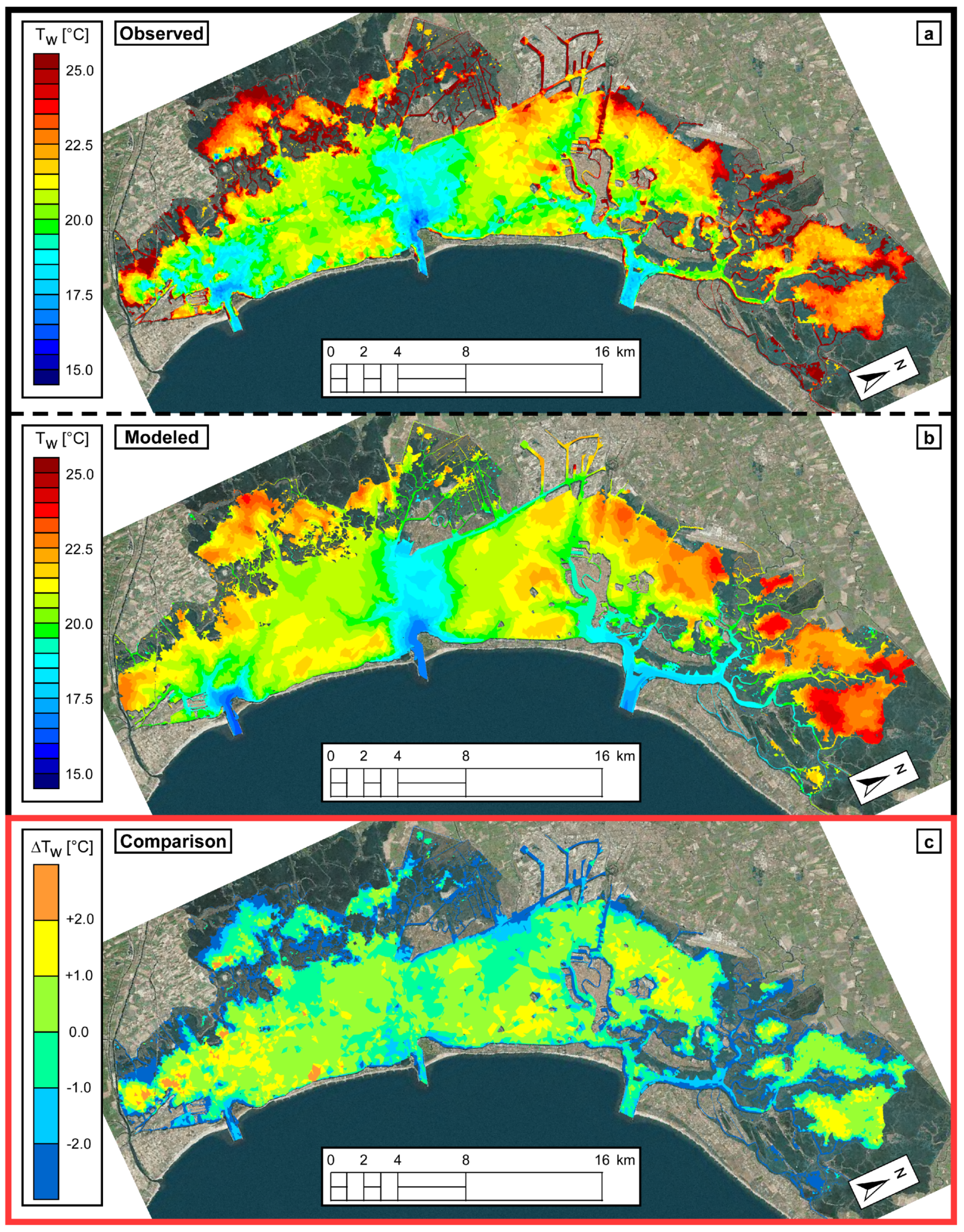
The successful comparison between the water temperature map obtained from the 9 May 2008 satellite image and that computed at the end of the model simulation (see Figure 7) further confirms the reliability of the model. The absolute difference between modeled and observed water temperature, $\mathsf{\Delta }{T}_w$, is lower than $1°\mathrm{C}$ in most of the water basin, especially on the tidal flats dominating the present landscape of the Venice lagoon. The model overestimates the satellite-derived water temperature by more than $1°\mathrm{C}$ in limited areas, which represent less than 9% of the wet surface of the lagoon. Overestimation of more than $2°\mathrm{C}$ affects only a negligible portion (about 0.7%) of the basin.

The observed overestimation of the water temperature can be ascribed to model limitations in computing the net vertical energy flux $H_{NET}$ and/or in describing the transport/diffusion process properly. Specifically, the assumption that the heat exchange at the SWI provides a negligible contribution to the total energy balance can be less realistic in the shallower areas. Accounting for this heat flux component in computing $H_{NET}$ could certainly improve the model accuracy but at the cost of an additional, not negligible, computational cost. Such an observation was further supported by an additional run we performed considering a much hotter period starting from a reliable description of the initial state of the system provided by a satellite image captured the 22 August 2011 (results not shown). The comparison of model results with point data are in line with those discussed herein (May 2008) over most of the lagoon with a slightly increased tendency in overestimating the water temperature in the innermost areas that seems to suggest a more relevant role potentially exerted by the heat fluxes at the SWI during the summer period.

Moreover, the simulation performed and discussed herein assumes a uniform spatial distribution of the meteorological forcings, accounting for their possible spatial variability that could further improve the estimation of the energy fluxes and, in turn, the description of the water temperature dynamics. To this point, it has to be noted that the numerical model already accounts for the spatial variability of the wind field adopting the interpolation technique of the available wind data proposed by Brocchini et al. [36], a method that could be applied also to the other meteorological data. However, only few measuring stations collecting meteorological data are available within the Venice lagoon and their distribution is not such to satisfactorily reconstruct their spatial variability.

The model seems to underestimate the water temperature in proximity of the border of the computational domain and on elements surrounded by dry areas, with negative values of $\mathsf{\Delta }{T}_w$ lower than $-1°\mathrm{C}$ and $-2°\mathrm{C}$ observed in about the 25% and the 16% of the wet surface of the lagoon, respectively. These differences, however, are more likely to be ascribed to misleading information inherent in the remotely sensed data than to model limitations. In fact, as already discussed in Section 2.4 and despite the buffer region used to mask satellite temperature maps along the coastline, the temperature retrieved from satellite images in these border areas (or in areas that are almost dry at the acquisition time) may be still influenced by the soil temperature of the neighboring surfaces. Moreover, the water temperature of areas close to human settlements (e.g., Venice, Murano, and Marghera) could be affected by the discharge of warm water as the byproduct of anthropic activities and not accounted for in the simulation.

In this regard, it is interesting to observe that the remotely sensed water temperature in front of the industrial estate of Marghera is higher than the modeled water temperature. Since the performed simulation does not account for any local heat source caused by the industrial activities, these temperature differences can be attributed to the use of the water resource for cooling purposes by the production facilities, as noticed in other studies [60]. This observation highlights how a combined use of modeling results and spatial distributed temperature data can provide useful insights about the impact of the thermal pollution due to industrial activities and can evaluate the effects due to possible anthropic uses of the water resource (e.g., hydrothermic systems to be used for cooling/warming purposes of buildings in Venice in order to overcome the architectural impact of the common conditioners).

Finally, it is important to point out that a higher accuracy in the estimation of the water temperature from satellite may further improve the results obtained with our method. Improved accuracy may be obtained using data from sensors that have at least two bands in the thermal portion of the spectrum, as for example AVHRR and MODIS. In these cases, split-window methods may be applied (i.e., [61]). Sensors that provide three or more bands in the TIR spectral range are also available (as for example ASTER), possibly providing the retrieval of surface temperature with even higher accuracies. The two main limitations in the use of these sensors for calibrating/validating hydrodynamic circulation-heat transport models of small and medium size tidal basins are (1) their limited spatial resolution (as for AVHRR and MODIS) and (2) the unavailability of images collected over the same target at short time intervals (as for ASTER). Landsat satellites have the advantage of both high spatial resolution and acquisition frequency; however, they provide just one thermal band. Therefore, an estimation of the parameters characterizing the atmosphere during the acquisition is needed in order to correct the signal of one single thermal band for atmospheric interference. In this study, we applied the Atmospheric Correction Parameter Calculator tool [55], which is applied to the entire image without taking into account the variability of water vapor and other atmospheric parameters that influence the retrieval of the correct sea surface temperature. We believe that such a variability is responsible for the variable difference between the temperature recorded at the probes and that calculated from satellite data. A pixel-by-pixel atmospheric correction method may reduce such effect [62]; however, high spatial resolution ancillary data are needed in order to correctly calculate (or simulate) the spatial variability of the atmospheric parameters. Such ancillary data may be retrieved from other sources, as suggested in the method proposed by Galve et al. [62] that uses the National Centers of Environmental Prediction (NCEP) profiles. Such an approach may improve the results obtained with our study; however, we speculate that, in our case, the efficacy of the method is limited by the very low spatial resolution of the NCEP profiles that are provided on a $1°\times 1°$ longitude/latitude grid every $6\mathrm{h}$. Based on all these considerations, we believe that the post-correction of the temperatures retrieved from satellite using the measurements performed by the ten probes spread across the Venice lagoon is the most accurate method for our case study. The future availability of sensors with two or more bands in the TIR domain and high spatial and temporal resolution may improve the situation.

5. Conclusions

The present study shows that the use of temperature data provided by satellite observations and in situ point measurements of water and meteorological parameters, combined with a spatially explicit and physics-based numerical model for hydro- and temperature dynamics, represents a powerful tool to investigate and describe the water temperature dynamics in shallow coastal environments.

Remotely sensed data and point observations are crucial for monitoring purposes since they provide different, complementary information: infrequent in time but spatially distributed the first ones, and continuous in time but sparse in space the second ones. In the integrated approach developed and tested with reference to the Venice Lagoon, data from these different sources have been used jointly to constrain a physics-based numerical model. The water temperatures computed by the model compare satisfactorily with both in situ measured time series and spatially distributed satellite data. The mean difference between modeled and computed water temperature at the end of a 7-day-long simulation is $1.27\pm 2.15°$C, with differences lower than $1°$C on about the 65% of the lagoon. Proven its reliability, the model can overcome the intrinsic limitations of different monitoring techniques by acting as a physical interpolator able to complete temperature information both in time and in space.

This tool can find applications in investigating scenarios related to anthropic possible uses of the water resource for warming/cooling purposes. Moreover, knowing the crucial role exerted by water temperature in many physical and biological processes, our results point out that the combined use of in situ point measures, remote sensing, and numerical modeling can be highly effective in understanding and estimating the eco-bio-morphodynamics evolution of shallow water coastal systems and in planning suitable managements procedures.