Prediction of Socio-Economic Indicators for Urban Planning Using VHR Satellite Imagery and Spatial Analysis

 ,
,  ,
, 
Abstract
:
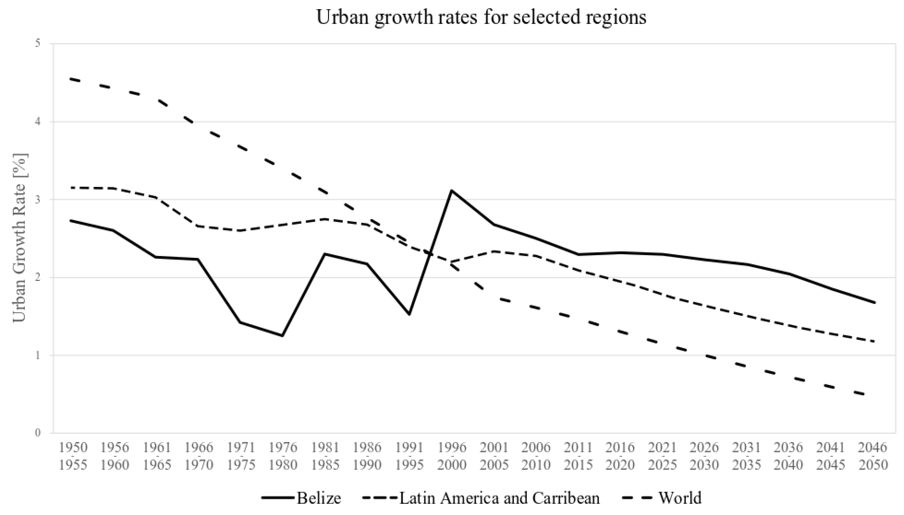
1. Introduction
2. Materials and Methods
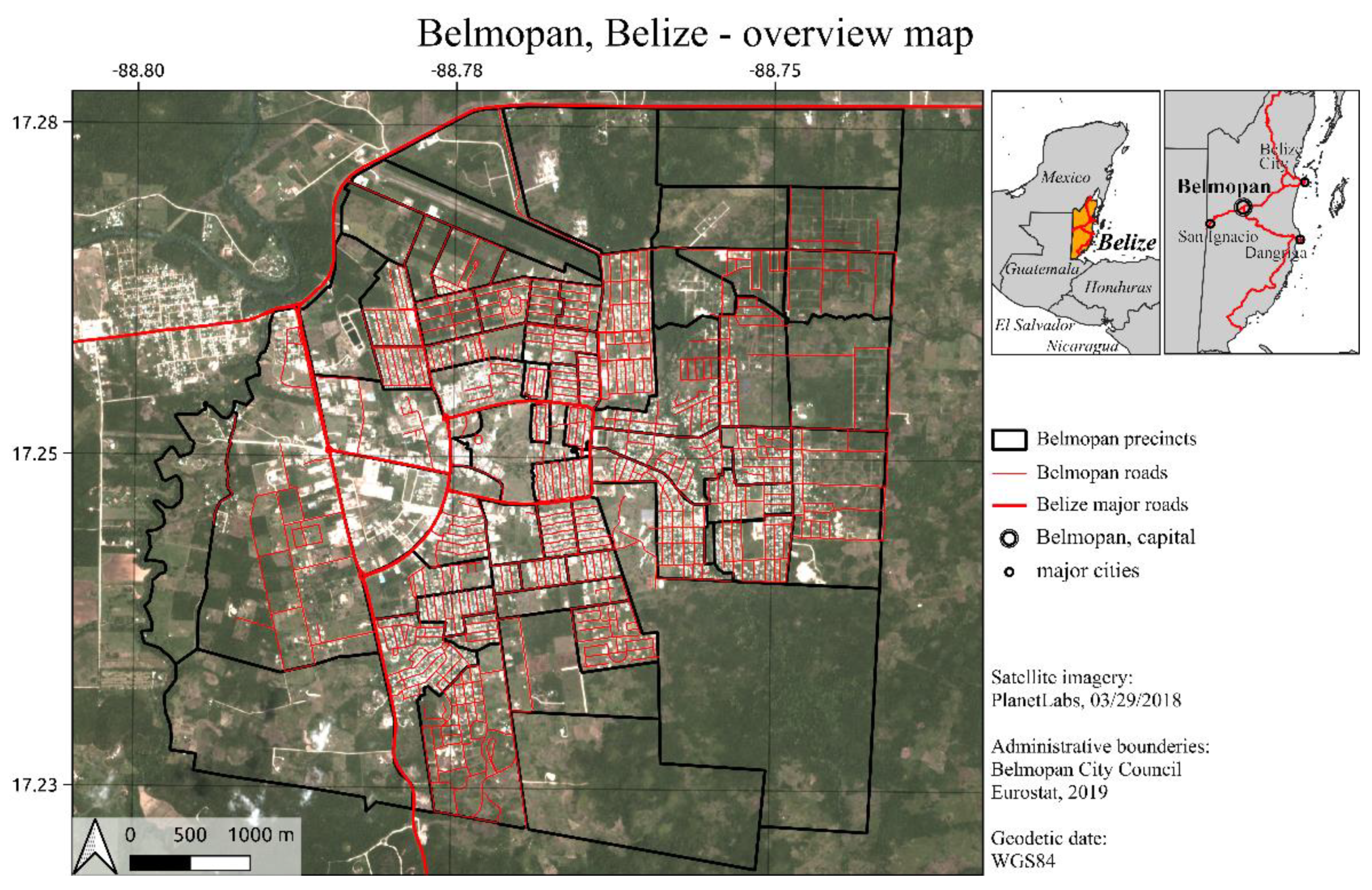
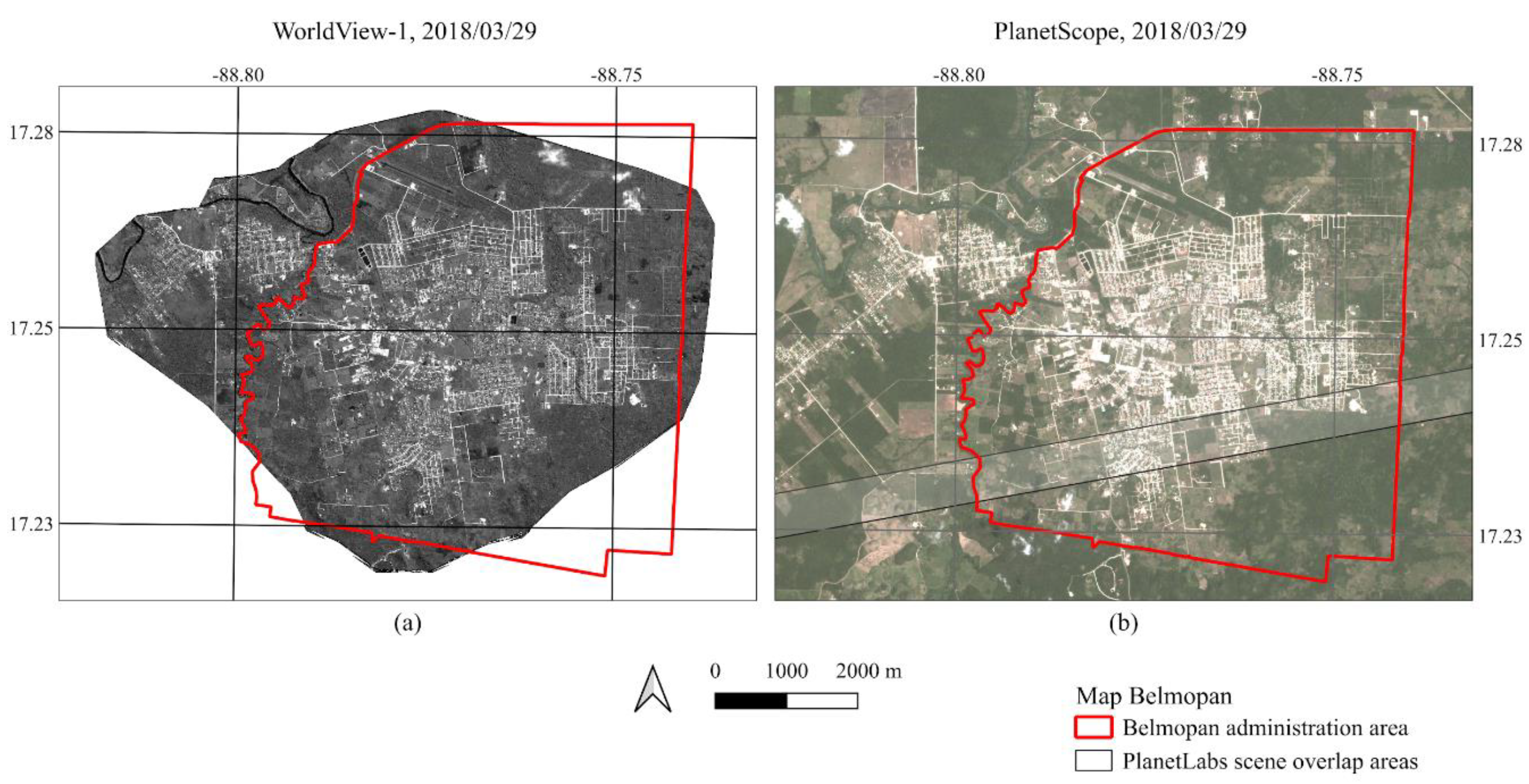
2.1. Study Area and Data
2.1.1. Study Area
2.1.2. VHR Imagery
2.1.3. HR Imagery
2.1.4. Ground Truthing Data
2.1.5. Auxiliary Data
2.1.6. Socio-Economic Interviews
- housing and infrastructure (type and devices of the house);
- specific information on the household (size, age structure, occupation, education, etc.);
- items, features and devices (assets) owned by the household;
- expenditures (on housing, food, health, etc.) of the household;
- food and buying habits of the household;
- income (amount, sources) of the household.
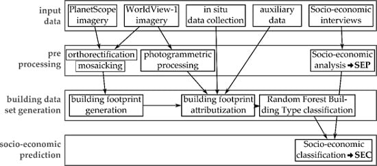
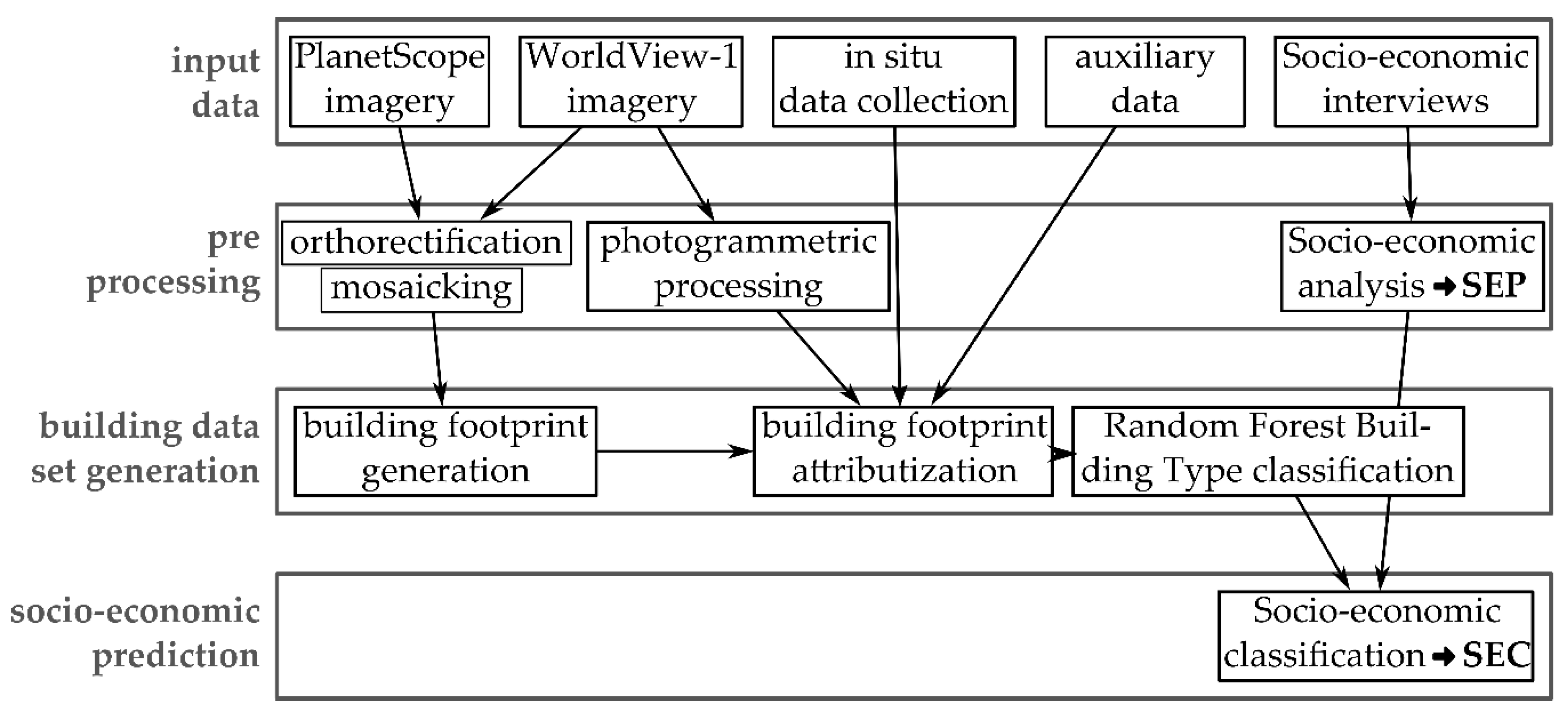
2.2. Methods
2.2.1. VHR Image Processing
2.2.2. Delineation of Building Footprints
2.2.3. HR Image Processing
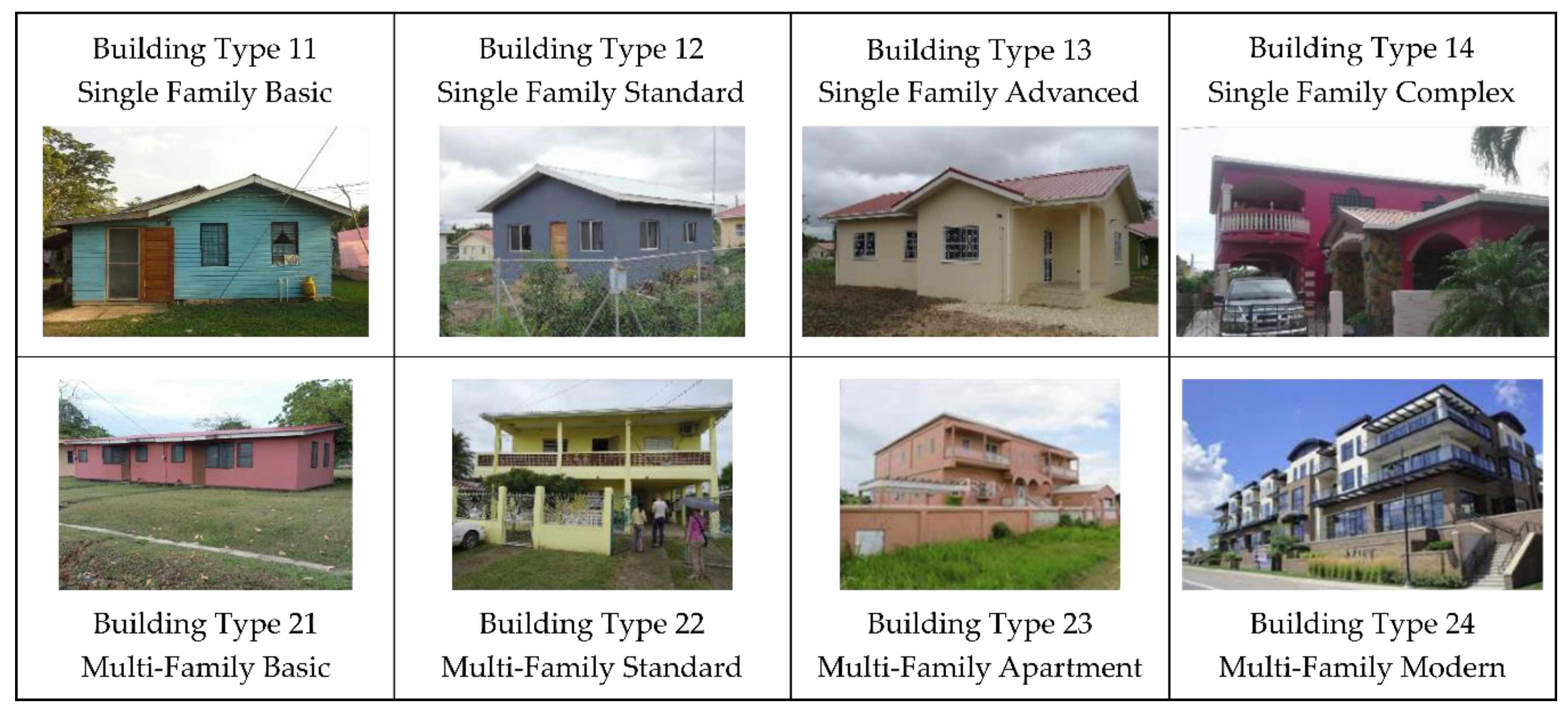
2.2.4. Definition of Building Typology
2.2.5. Classification of Building Types
- Geometry features (n = 6): area; perimeter; number of corners; shape ratio (area/perimeter); shape index [89]; average height (Section 2.2.1.).
- Distance features (Euclidean, n = 8): roads; paved roads; bus lines; parcels of land use commercial; parcels of land use education; parcels of land use green spaces; parcels of land use industry; parcels of land use public.
- Density features (n = 5): average building density within a radius of 150 and 250 m; absolute number of buildings within 50, 100, and 200 m.
- Land use features (according to the official plan provided by the city council, n = 2). 10 parcel classes: agriculture, commercial, education, green space, industrial, mixed use, public/institutional, residential, utilities, vacant. Four sector classes: built-up, developing, vacant/agriculture/forest, university.
- Spectral features (average per polygon, n = 4): HR red; HR green; HR blue; HR infrared.
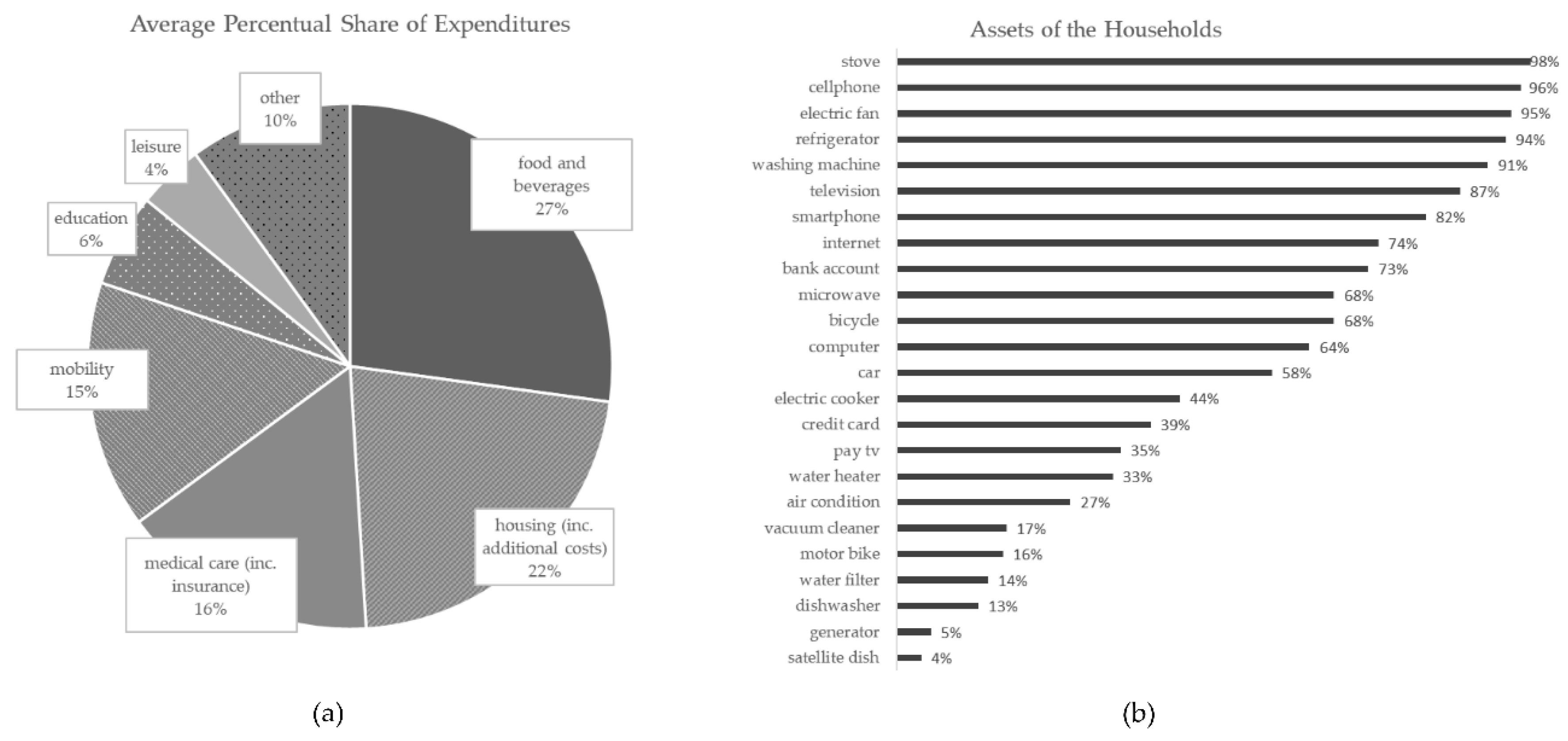
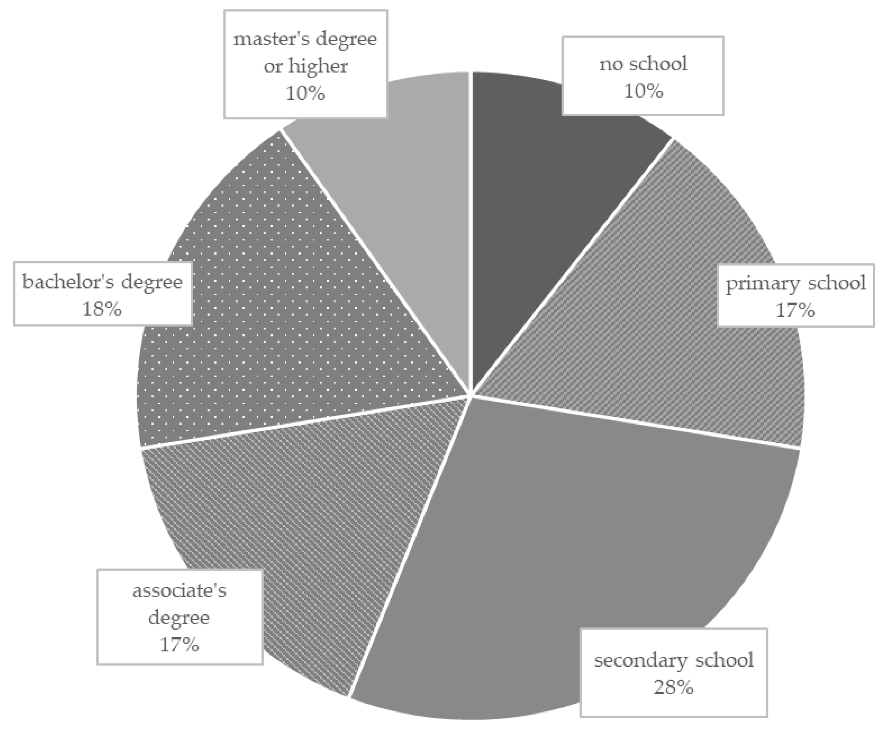
2.2.6. Processing of Socio-Economic Data
- Expenditures.
- Educational level.
- Household assets (owned items).
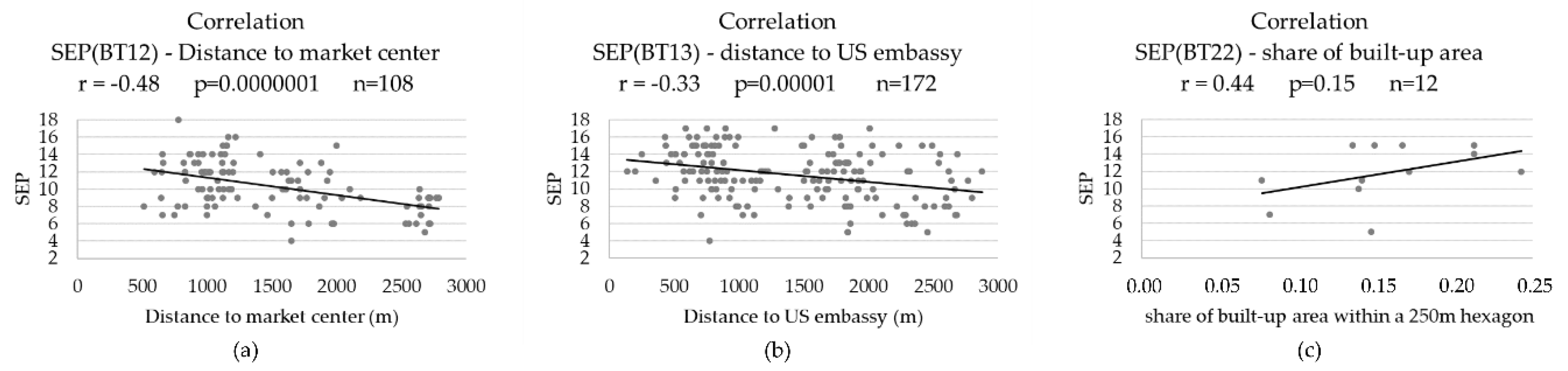
2.2.7. Classification and Prediction of Socio-Economic Data
- distance to main roads (ring road)
- distance to administrative center (city administration);
- distance to places of education;
- distance to market center (market square);
- distance to US Embassy;
- building density;
- vegetation density.
3. Results
3.1. Building Detection
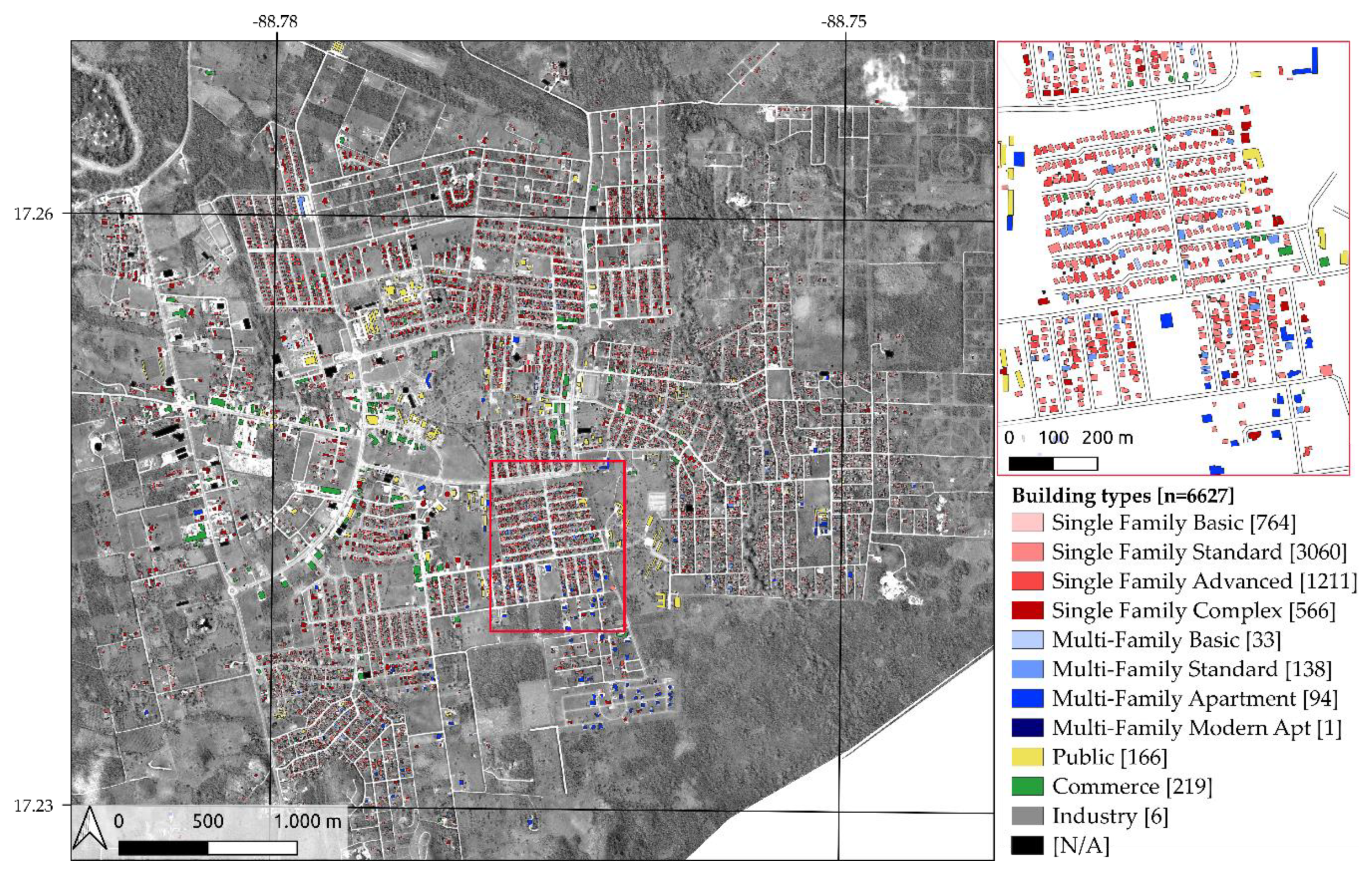
3.2. Building Type Classification
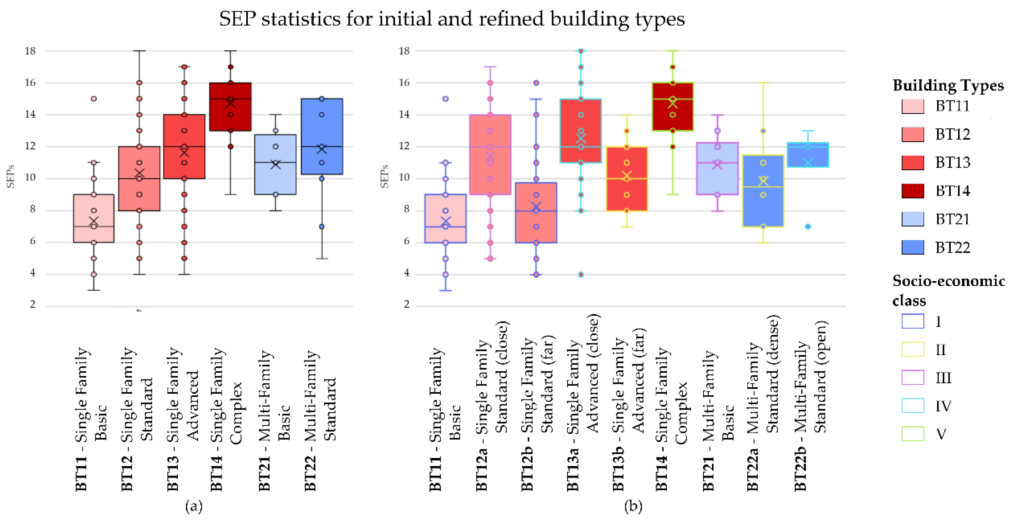
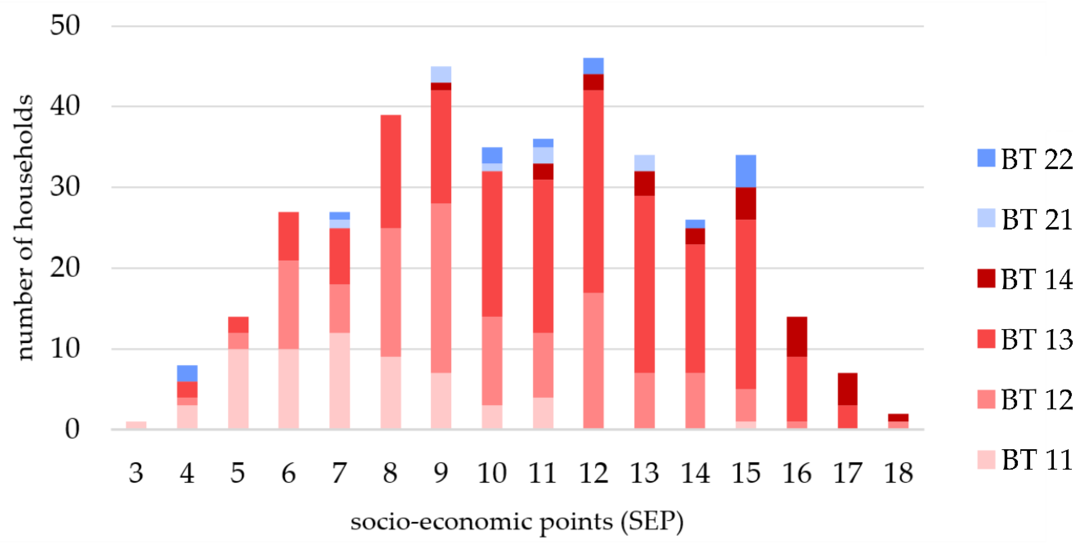
3.3. Socio-Economic Points Determination
3.4. Class Generation and Extrapolation
- To predict socio-economic relevant planning values on a single building scale based on building type;
- To avoid a false impression of precision;
- Not to publish detailed sensitive information on resident’s socio-economic status at a single building level.
4. Discussion
- The establishment of the building typology needs to be adapted for individual case cities. High variations in building types can even exist within countries;
- The generation of socio-economic information and a socio-economic scaling, SEP in our study, must be based on local information and current surveys;
- This work indirectly confirms findings of previous studies on location-dependent land value [31,94] through high variation of SEP within single building types. By applying spatial measures, building types can be disaggregated to achieve building types homogenous in SEPs. To identify reference points of urban function, local knowledge is needed as well.
5. Conclusions
Author Contributions
Funding
Acknowledgments
Conflicts of Interest
Appendix A. Building Heights Validation

Appendix B. Manual Refinement of Building Type Classifications
- uninhabited
- “btype_complete” like ‘%Single%’ and “shp_area” > 510 and “shp_corners” <= 5
- “shp_area” < 30
- Single Family Advanced
- “btype_complete” = ‘Single Family Standard’ and “hgt_building” > 4 and “shp_area” > 150
Appendix C. Figure Showing Socio-Economic Points Composition per Building Type

Appendix D. Table Showing Correlation between SEP and Distances from Urban Points of Centrality

| SEP (Building Type Level) | r Ringroad | r Center | r US Embassy | r Built-Up 250 m |
|---|---|---|---|---|
| 12—Single Family Standard | −0.47 (p = 1.8 * 10−7) | −0.48 (p = 1.1 * 10−7) | −0.44 (p = 1.4 * 10−6) | 0.29 (p = 0.002) |
| 13—Single Family Advanced | −0.19 (p = 0.01) | −0.27 (p = 0.0004) | −0.33 (p = 1.2 * 10−5) | 0.05 (p = 0.5) |
| 22—Multi-Family Standard | −0.30 (p = 0.33) | −0.43 (p = 0.15) | −0.19 (p = 0.55) | 0.44 (p = 0.15) |
Appendix E. Overview on Parameters for Disaggregating Building Types 12, 13, and 22
| Initial Building Types | n | Mean SEP | Standard Deviation SEP | Threshold |
| 12—Single Family Standard | 108 | 10.4 | 2.79 | 988 m |
| 13—Single Family Advanced | 172 | 11.6 | 2.94 | 1018 m |
| 22—Multi-Family Standard | 12 | 11.8 | 3.30 | 0.125 |
| Refined Building types | n | Mean SEP | Standard Deviation SEP | |
| 11—Single Family basic | 55 | 7.3 | 2.2 | |
| 12a—Single Family Standard close | 74 | 11.3 | 2.59 | |
| 12b—Single Family Standard far | 34 | 8.3 | 1.99 | |
| 13a—Single Family Advanced close | 69 | 12.8 | 2.6 | |
| 13b—Single Family Advanced far | 103 | 10.9 | 2.9 | |
| 14—Single Family complex | 24 | 14.7 | 2.1 | |
| 22a—Multi-Family Advanced open | 6 | 13.8 | 1.47 | |
| 22b—Multi-Family Advanced dense | 6 | 9.8 | 3.48 | |
| 23—Multi-Family Apartment | 1 | 15 | - |
References
- United Nations Department of Economic Social Affairs. World Urbanization Prospects: The 2018 Revision; United Nations: New York, NY, USA, 2018. [Google Scholar]
- Cohen, B. Urbanization in developing countries: Current trends, future projections, and key challenges for sustainability. Technol. Soc. 2006, 28, 63–80. [Google Scholar] [CrossRef]
- UN General Assembly. Transforming Our World: The 2030 Agenda for Sustainable Development; United Nations: New York, NY, USA, 2015. [Google Scholar]
- Guterres, A. Actions for the Further Implementation of the Programme of Action of the International Conference on Population and Development: Monitoring of Population Programmes, Focusing on Sustainable Cities, Human Mobility and International Migration; United Nations Economic and Social Council: New York, NY, USA, 2018.
- United Nations Human Settlements Programme. Planning Sustainable Cities: Global Report on Human Settlements 2009; Earthscan: London, UK, 2009. [Google Scholar]
- Oribe-Garcia, I.; Kamara-Esteban, O.; Martin, C.; Macarulla-Arenaza, A.M.; Alonso-Vicario, A. Identification of influencing municipal characteristics regarding household waste generation and their forecasting ability in Biscay. Waste Manag. 2015, 39, 26–34. [Google Scholar] [CrossRef] [PubMed] [Green Version]
- Khan, D.; Kumar, A.; Samadder, S.R. Impact of socioeconomic status on municipal solid waste generation rate. Waste Manag. 2016, 49, 15–25. [Google Scholar] [CrossRef] [PubMed]
- Xu, L.; Lin, T.; Xu, Y.; Xiao, L.; Ye, Z.; Cui, S. Path analysis of factors influencing household solid waste generation: A case study of Xiamen Island, China. J. Mater. Cycles Waste Manag. 2016, 18, 377–384. [Google Scholar] [CrossRef]
- Bosire, E.; Oindo, B.; Atieno, J.V. Modeling Household Solid Waste Generation in Urban Estates Using SocioEconomic and Demographic Data; Maseno University: Kisumu City, Kenya, 2017. [Google Scholar]
- Jones, R.V.; Fuertes, A.; Lomas, K.J. The socio-economic, dwelling and appliance related factors affecting electricity consumption in domestic buildings. Renew. Sustain. Energy Rev. 2015, 43, 901–917. [Google Scholar] [CrossRef] [Green Version]
- Brown de Colstoun, E.C.; Huang, C.; Wang, P.; Tilton, J.C.; Tan, B.; Phillips, J.; Niemczura, S.; Ling, P.-Y.; Wolfe, R.E. Global Man-made Impervious Surface (GMIS) Dataset from Landsat; NASA Socioeconomic Data and Applications Center (SEDAC): Palisades, NY, USA, 2017. [Google Scholar]
- Zhou, Y.; Smith, S.J.; Zhao, K.; Imhoff, M.; Thomson, A.; Bond-Lamberty, B.; Asrar, G.R.; Zhang, X.; He, C.; Elvidge, C.D. A global map of urban extent from nightlights. Environ. Res. Lett. 2015, 10, 054011. [Google Scholar] [CrossRef]
- Esch, T.; Marconcini, M.; Felbier, A.; Roth, A.; Heldens, W.; Huber, M.; Schwinger, M.; Taubenböck, H.; Müller, A.; Dech, S. Urban Footprint Processor—Fully Automated Processing Chain Generating Settlement Masks From Global Data of the TanDEM-X Mission. IEEE Geosci. Remote Sens. Lett. 2013, 10, 1617–1621. [Google Scholar] [CrossRef] [Green Version]
- Esch, T.; Heldens, W.; Hirner, A.; Keil, M.; Marconcini, M.; Roth, A.; Zeidler, J.; Dech, S.; Strano, E. Breaking new ground in mapping human settlements from space–The Global Urban Footprint. ISPRS J. Photogramm. Remote Sens. 2017, 134, 30–42. [Google Scholar] [CrossRef] [Green Version]
- Marconcini, M.; Metz-Marconcini, A.; Uereyen, S.; Palacios Lopez, D.; Hanke, W.; Bachofer, F.; Zeidler, J.; Esch, T.; Gorelick, N.; Kakarla, A.; et al. Outlining Where Humans Live—The World Settlement Footprint 2015. Available online: https://arxiv.org/abs/1910.12707 (accessed on 11 November 2019).
- Warth, G.; Braun, A.; Bödinger, C.; Hochschild, V.; Bachofer, F. DSM-based identification of changes in highly dynamic urban agglomerations. Eur. J. Remote Sens. 2019, 52, 322–334. [Google Scholar] [CrossRef] [Green Version]
- Braun, A.; Warth, G.; Bachofer, F.; Bui, T.; Tran, H.; Hochschild, V. Changes in the building stock of DaNang between 2015 and 2017. Data 2020, 5, 42. [Google Scholar] [CrossRef]
- Blaschke, T. Object based image analysis for remote sensing. ISPRS J. Photogramm. Remote Sens. 2010, 65, 2–16. [Google Scholar] [CrossRef] [Green Version]
- Dey, V.; Zhang, Y.; Zhong, M. Building detection from pan-sharpened GeoEye-1 satellite imagery using context based multi-level image segmentation. In Proceedings of the 2011 International Symposium on Image and Data Fusion, Tengchong, China, 9 August 2011; pp. 1–4. [Google Scholar]
- Grippa, T.; Lennert, M.; Beaumont, B.; Vanhuysse, S.; Stephenne, N.; Wolff, E. An Open-Source Semi-Automated Processing Chain for Urban Object-Based Classification. Remote Sens. 2017, 9, 358. [Google Scholar] [CrossRef] [Green Version]
- Banzhaf, E.; Kollai, H.; Kindler, A. Mapping urban grey and green structures for liveable cities using a 3D enhanced OBIA approach and vital statistics. Geocarto Int. 2018, 35, 1–18. [Google Scholar] [CrossRef]
- Sari, N.M.; Kushardono, D. Quality Analysis of Single Tree Object with OBIA and Vegetation Index from LAPAN Surveillance Aircraft Multispectral Data in Urban Area. Geoplanning J. Geomat. Plan. 2016, 3, 93–106. [Google Scholar] [CrossRef] [Green Version]
- Labib, S.M.; Harris, A. The potentials of Sentinel-2 and LandSat-8 data in green infrastructure extraction, using object based image analysis (OBIA) method. Eur. J. Remote Sens. 2018, 51, 231–240. [Google Scholar] [CrossRef]
- Banzhaf, E.; de la Barrera, F. Evaluating public green spaces for the quality of life in cities by integrating RS mapping tools and social science techniques. In Proceedings of the 2017 Joint Urban Remote Sensing Event (JURSE), Dubai, UAE, 6–8 March 2017; pp. 1–4. [Google Scholar]
- LeCun, Y.; Huang, F.J.; Bottou, L. Learning methods for generic object recognition with invariance to pose and lighting. In Proceedings of the 2004 IEEE Computer Society Conference on Computer Vision and Pattern Recognition, 2004. CVPR 2004, Washington, DC, USA, 27 June–2 July 2004; pp. II–104. [Google Scholar]
- Vakalopoulou, M.; Karantzalos, K.; Komodakis, N.; Paragios, N. Building detection in very high resolution multispectral data with deep learning features. In Proceedings of the 2015 IEEE International Geoscience and Remote Sensing Symposium (IGARSS), Milan, Italy, 26–31 July 2015; pp. 1873–1876. [Google Scholar]
- Persello, C.; Stein, A. Deep Fully Convolutional Networks for the Detection of Informal Settlements in VHR Images. IEEE Geosci. Remote Sens. Lett. 2017, 14, 2325–2329. [Google Scholar] [CrossRef]
- Liu, R.; Kuffer, M.; Persello, C. The Temporal Dynamics of Slums Employing a CNN-Based Change Detection Approach. Remote Sens. 2019, 11, 2844. [Google Scholar] [CrossRef] [Green Version]
- Xia, X.; Persello, C.; Koeva, M. Deep Fully Convolutional Networks for Cadastral Boundary Detection from UAV Images. Remote Sens. 2019, 11, 1725. [Google Scholar] [CrossRef] [Green Version]
- Zhu, X.X.; Tuia, D.; Mou, L.; Xia, G.; Zhang, L.; Xu, F.; Fraundorfer, F. Deep Learning in Remote Sensing: A Comprehensive Review and List of Resources. IEEE Geosci. Remote Sens. Mag. 2017, 5, 8–36. [Google Scholar] [CrossRef] [Green Version]
- Brimble, P.; McSharry, P.; Bachofer, F.; Bower, J.; Braun, A. Using Machine Learning and Remote Sensing to Value Property in Kigali; The International Growth Centre: London, UK, 2020. [Google Scholar]
- Mikhail, E.M.; Bethel, J.S.; McGlone, J.C. Introduction to Modern Photogrammetry; Wiley: New York, NY, USA, 2001. [Google Scholar]
- Bachofer, F. Assessment of building heights from pléiades satellite imagery for the Nyarugenge sector, Kigali, Rwanda. Rwanda J. 2017, 1. [Google Scholar] [CrossRef] [Green Version]
- Dong, P.; Chen, Q. LiDAR Remote Sensing and Applications; CRC Press: Boca Raton, FL, USA, 2017. [Google Scholar]
- Liu, L.; Coops, N.C.; Aven, N.W.; Pang, Y. Mapping urban tree species using integrated airborne hyperspectral and LiDAR remote sensing data. Remote Sens. Environ. 2017, 200, 170–182. [Google Scholar] [CrossRef]
- Alonzo, M.; McFadden, J.P.; Nowak, D.J.; Roberts, D.A. Mapping urban forest structure and function using hyperspectral imagery and lidar data. Urban For. Urban Green. 2016, 17, 135–147. [Google Scholar] [CrossRef] [Green Version]
- Giannico, V.; Lafortezza, R.; John, R.; Sanesi, G.; Pesola, L.; Chen, J. Estimating Stand Volume and Above-Ground Biomass of Urban Forests Using LiDAR. Remote Sens. 2016, 8, 339. [Google Scholar] [CrossRef] [Green Version]
- Lafortezza, R.; Giannico, V. Combining high-resolution images and LiDAR data to model ecosystem services perception in compact urban systems. Ecol. Indic. 2019, 96, 87–98. [Google Scholar] [CrossRef]
- Zhang, H.; Lin, H.; Wang, Y. A new scheme for urban impervious surface classification from SAR images. ISPRS J. Photogramm. Remote Sens. 2018, 139, 103–118. [Google Scholar] [CrossRef]
- Crosetto, M.; Castillo, M.; Arbiol, R. Urban subsidence monitoring using radar interferometry. Photogramm. Eng. Remote Sens. 2003, 69, 775–783. [Google Scholar] [CrossRef]
- Potin, P.; Rosich, B.; Miranda, N.; Grimont, P.; Shurmer, I.; O’Connell, A.; Krassenburg, M.; Gratadour, J.-B. Copernicus Sentinel-1 Constellation Mission Operations Status. In Proceedings of the IGARSS-2019 IEEE International Geoscience and Remote Sensing Symposium, Yokohama, Japan, 28 July–2 August 2019; pp. 5385–5388. [Google Scholar]
- Gabriel, A.K.; Goldstein, R.M.; Zebker, H.A. Mapping small elevation changes over large areas: Differential radar interferometry. J. Geophys. Res. Solid Earth 1989, 94, 9183–9191. [Google Scholar] [CrossRef]
- Notti, D.; Mateos, R.M.; Monserrat, O.; Devanthéry, N.; Peinado, T.; Roldán, F.J.; Fernández-Chacón, F.; Galve, J.P.; Lamas, F.; Azañón, J.M. Lithological control of land subsidence induced by groundwater withdrawal in new urban areas (Granada Basin, SE Spain). Multiband DInSAR monitoring. Hydrol. Process. 2016, 30, 2317–2331. [Google Scholar] [CrossRef]
- Cascini, L.; Ferlisi, S.; Fornaro, G.; Lanari, R.; Peduto, D.; Zeni, G. Subsidence monitoring in Sarno urban area via multi-temporal DInSAR technique. Int. J. Remote Sens. 2006, 27, 1709–1716. [Google Scholar] [CrossRef]
- Chaussard, E.; Amelung, F.; Abidin, H.; Hong, S.-H. Sinking cities in Indonesia: ALOS PALSAR detects rapid subsidence due to groundwater and gas extraction. Remote Sens. Environ. 2013, 128, 150–161. [Google Scholar] [CrossRef]
- Tesauro, M.; Berardino, P.; Lanari, R.; Sansosti, E.; Fornaro, G.; Franceschetti, G. Urban subsidence inside the city of Napoli (Italy) Observed by satellite radar interferometry. Geophys. Res. Lett. 2000, 27, 1961–1964. [Google Scholar] [CrossRef]
- Delgado Blasco, J.M.; Foumelis, M.; Stewart, C.; Hooper, A. Measuring Urban Subsidence in the Rome Metropolitan Area (Italy) with Sentinel-1 SNAP-StaMPS Persistent Scatterer Interferometry. Remote Sens. 2019, 11, 129. [Google Scholar] [CrossRef] [Green Version]
- Wang, H.; Feng, G.; Xu, B.; Yu, Y.; Li, Z.; Du, Y.; Zhu, J. Deriving spatio-temporal development of ground subsidence due to subway construction and operation in delta regions with PS-InSAR data: A case study in Guangzhou, China. Remote Sens. 2017, 9, 1004. [Google Scholar] [CrossRef] [Green Version]
- Fornaro, G.; Lombardini, F.; Pauciullo, A.; Reale, D.; Viviani, F. Tomographic Processing of Interferometric SAR Data: Developments, applications, and future research perspectives. IEEE Signal Process. Mag. 2014, 31, 41–50. [Google Scholar] [CrossRef]
- Budillon, A.; Crosetto, M.; Johnsy, A.C.; Monserrat, O.; Krishnakumar, V.; Schirinzi, G. Comparison of Persistent Scatterer Interferometry and SAR Tomography Using Sentinel-1 in Urban Environment. Remote Sens. 2018, 10, 1986. [Google Scholar] [CrossRef] [Green Version]
- Crosetto, M.; Budillon, A.; Monserrat, O. Urban Deformation Monitoring using Persistent Scatterer Interferometry and SAR tomography; MDPI: Basel, Switzerland, 2019. [Google Scholar]
- Shi, Y.; Wang, Y.; Zhu, X.X.; Bamler, R. Non-Local SAR Tomography for Large-Scale Urban Mapping. In Proceedings of the IGARSS 2019–2019 IEEE International Geoscience and Remote Sensing Symposium, Yokohama, Japan, 28 July–2 August 2019; pp. 5197–5200. [Google Scholar]
- Li, Y.; Martinis, S.; Wieland, M.; Schlaffer, S.; Natsuaki, R. Urban Flood Mapping Using SAR Intensity and Interferometric Coherence via Bayesian Network Fusion. Remote Sens. 2019, 11, 2231. [Google Scholar] [CrossRef] [Green Version]
- Kuffer, M.; Pfeffer, K.; Sliuzas, R. Slums from space—15 years of slum mapping using remote sensing. Remote Sens. 2016, 8, 455. [Google Scholar] [CrossRef] [Green Version]
- Kuffer, M.; Pfeffer, K.; Sliuzas, R.; Baud, I. Extraction of slum areas from VHR imagery using GLCM variance. IEEE J. Sel. Top. Appl. Earth Obs. Remote Sens. 2016, 9, 1830–1840. [Google Scholar] [CrossRef]
- Jensen, J.R.; Cowen, D.C. Remote sensing of urban/suburban infrastructure and socio-economic attributes. Photogramm. Eng. Remote Sens. 1999, 65, 611–622. [Google Scholar]
- Lo, C.P.; Faber, B.J. Integration of Landsat Thematic Mapper and census data for quality of life assessment. Remote Sens. Environ. 1997, 62, 143–157. [Google Scholar] [CrossRef]
- Martinuzzi, S.; Ramos-González, O.M.; Muñoz-Erickson, T.A.; Locke, D.H.; Lugo, A.E.; Radeloff, V.C. Vegetation cover in relation to socioeconomic factors in a tropical city assessed from sub-meter resolution imagery. Ecol. Appl. 2018, 28, 681–693. [Google Scholar] [CrossRef] [PubMed]
- Haas, J.; Ban, Y. Sentinel-1A SAR and sentinel-2A MSI data fusion for urban ecosystem service mapping. Remote Sens. Appl. Soc. Environ. 2017, 8, 41–53. [Google Scholar] [CrossRef]
- Yang, Y.; Wu, T.; Wang, S.; Li, J.; Muhanmmad, F. The NDVI-CV Method for Mapping Evergreen Trees in Complex Urban Areas Using Reconstructed Landsat 8 Time-Series Data. Forests 2019, 10, 139. [Google Scholar] [CrossRef] [Green Version]
- Lin, D.; Gold, H.T.; Schreiber, D.; Leichman, L.P.; Sherman, S.E.; Becker, D.J. Impact of socioeconomic status on survival for patients with anal cancer. Cancer 2018, 124, 1791–1797. [Google Scholar] [CrossRef]
- Rosengren, A.; Smyth, A.; Rangarajan, S.; Ramasundarahettige, C.; Bangdiwala, S.I.; AlHabib, K.F.; Avezum, A.; Bengtsson Boström, K.; Chifamba, J.; Gulec, S.; et al. Socioeconomic status and risk of cardiovascular disease in 20 low-income, middle-income, and high-income countries: The Prospective Urban Rural Epidemiologic (PURE) study. Lancet Glob. Health 2019, 7, e748–e760. [Google Scholar] [CrossRef] [Green Version]
- Kim, S.w.; Kim, E.J.; Wagaman, A.; Fong, V.L. A longitudinal mixed methods study of parents’ socioeconomic status and children’s educational attainment in Dalian City, China. Int. J. Educ. Dev. 2017, 52, 111–121. [Google Scholar] [CrossRef]
- McKenzie, D.J. Measuring inequality with asset indicators. J. Popul. Econ. 2005, 18, 229–260. [Google Scholar] [CrossRef]
- Renard, F.; Devleesschauwer, B.; Speybroeck, N.; Deboosere, P. Monitoring health inequalities when the socio-economic composition changes: Are the slope and relative indices of inequality appropriate? Results of a simulation study. BMC Public Health 2019, 19, 662. [Google Scholar] [CrossRef] [Green Version]
- Hoffmann, R.; Kröger, H.; Pakpahan, E. Pathways between socioeconomic status and health: Does health selection or social causation dominate in Europe? Adv. Life Course Res. 2018, 36, 23–36. [Google Scholar] [CrossRef]
- Tighe, L.; Webster, N.J. The Influence of Socioeconomic Status on health and Well-Being: Comparing Diverse Trajectories. Innov. Aging 2017, 1, 983–984. [Google Scholar] [CrossRef] [Green Version]
- Kivimäki, M.; Batty, G.D.; Pentti, J.; Shipley, M.J.; Sipilä, P.N.; Nyberg, S.T.; Suominen, S.B.; Oksanen, T.; Stenholm, S.; Virtanen, M. Association between socioeconomic status and the development of mental and physical health conditions in adulthood: A multi-cohort study. Lancet Public Health 2020, 5, e140–e149. [Google Scholar] [CrossRef] [Green Version]
- Lampert, T.; Kroll, L.E.; Kuntz, B.; Hoebel, J. Gesundheitliche Ungleichheit in Deutschland und im Internationalen Vergleich: Zeitliche Entwicklungen und Trends; Robert-Koch-Institut: Berlin, Germany, 2018. [Google Scholar]
- Guterres, A. Sustainable Cities, Human Mobility and Internationalmigration; United Nations Economic and Social Council: New York, NY, USA, 2018.
- United Nations Human Settlements Programme. Belmopan Urban Development. Towards a Sustainable Garden City; Earthscan: London, UK, 2017. [Google Scholar]
- Statistical Institute of Belize. Annual Report 2018–19; Statistical Institute of Belize: Belmopan, Belize, 2019. [Google Scholar]
- Kaza, S.; Yao, L.; Bhada-Tata, P.; Van Woerden, F. What a Waste 2.0: A Global Snapshot of Solid Waste Management to 2050; The World Bank: Washington, DC, USA, 2018. [Google Scholar]
- Airbus Defence and Space. Pléiades Neo. Trusted Intelligence. Available online: https://www.intelligence-airbusds.com/en/8671-pleiades-neo-trusted-intelligence (accessed on 11 November 2019).
- Maxar. WorldView Legion. Our Next-generation Constellation. Available online: https://www.maxar.com/splash/worldview-legion (accessed on 12 February 2020).
- Kearns, K.C. Belmopan: Perspective on a new capital. Geogr. Rev. 1973, 63, 147–169. [Google Scholar] [CrossRef]
- Friesner, J. Hurricanes and the Forests of Belize; Forest Planning and Management Project; Ministry of Natural Resources: Belmopan, Belize, 1993. [Google Scholar]
- Statistical Institute of Belize. Annual Report 2017-18; Statistical Institute of Belize: Belmopan, Belize, 2018. [Google Scholar]
- DigitalGlobe. WorldView-1. Available online: https://www.euspaceimaging.com/wp-content/uploads/2018/08/WorldView1-DS-WV1_V02.pdf (accessed on 3 December 2019).
- Planet Team. Planet Application Program Interface: In Space for Life on Earth; San Francisco. 2017. Available online: https://api.planet.com (accessed on 2 February 2019).
- Planet. Planet Imagery Product Specification: Planetscope & Rapideye. Available online: https://www.planet.com/products/satellite-imagery/files/1610.06_Spec%20Sheet_Combined_Imagery_Product_Letter_ENGv1.pdf (accessed on 1 September 2019).
- Pham, P. KoBo Toolbox. In Proceedings of the Measure GIS Working Group Meeting, Rosslyn, VA, USA, 26 June 2012. [Google Scholar]
- Haklay, M.; Weber, P. Openstreetmap: User-generated street maps. IEEE Pervasive Comput. 2008, 7, 12–18. [Google Scholar] [CrossRef] [Green Version]
- Hexagon. Erdas Imagine 2018. Available online: https://download.hexagongeospatial.com/en/downloads/imagine/erdas-imagine-2018 (accessed on 11 January 2019).
- Legner, S. JOSM-Java OpenStreetMap Editor. In Proceedings of the FOSSGIS 2012, Dessau, Germany, 20–22 March 2012. [Google Scholar]
- Hashim, H.; Abd Latif, Z.; Adnan, N.A. Urban Vegetation Classifiction With NDVI Threshold Value Method with Very High Resolution (VHR) Pleiades Imagery. Int. Arch. Photogramm. Remote Sens. Spat. Inf. Sci. 2019, XLII-4/W16, 237–240. [Google Scholar] [CrossRef] [Green Version]
- Vetter-Gindele, J.; Braun, A.; Warth, G.; Bui, T.T.; Bachofer, F.; Eltrop, L. Assessment of Household Solid Waste Generation and Composition by Building Type in Da Nang, Vietnam. Resources 2019, 8, 171. [Google Scholar] [CrossRef] [Green Version]
- Point2homes. 2-Storey House. Available online: https://www.point2homes.com (accessed on 13 December 2019).
- Lang, S.; Blaschke, T. Landschaftsanalyse mit GIS; Ulmer: Stuttgart, Germany, 2007; p. 405. [Google Scholar]
- Breiman, L. Random Forests. Mach. Learn. 2001, 45, 5–32. [Google Scholar] [CrossRef] [Green Version]
- Winkler, J.; Stolzenberg, H. Der Sozialschichtindex im Bundes-Gesundheitssurvey. Gesundheitswesen 1998, 61, 178–183. [Google Scholar]
- Singh, T.; Sharma, S.; Nagesh, S. Socio-economic status scales updated for 2017. Int. J. Res. Med. Sci. 2017, 5, 3264–3267. [Google Scholar] [CrossRef] [Green Version]
- Biewen, M.; Juhasz, A. Direct Estimation of Equivalence Scales and More Evidence on Independence of Base. Oxf. Bull. Econ. Stat. 2017, 79, 875–905. [Google Scholar] [CrossRef]
- Kau, J.B.; Sirmans, C.F. Urban land value functions and the price elasticity of demand for housing. J. Urban Econ. 1979, 6, 112–121. [Google Scholar] [CrossRef]
- Pascascio, K.; (Belmopan City Council, Belmopan, Belize). Personal communication, 2019.
- Zhu, Z.; Zhou, Y.; Seto, K.C.; Stokes, E.C.; Deng, C.; Pickett, S.T.A.; Taubenböck, H. Understanding an urbanizing planet: Strategic directions for remote sensing. Remote Sens. Environ. 2019, 228, 164–182. [Google Scholar] [CrossRef]
- Nex, F.; Remondino, F. UAV for 3D mapping applications: A review. Appl. Geomat. 2014, 6, 1–15. [Google Scholar] [CrossRef]

| WorldView-1 Stereo Pair 1 | WorldView-1 Stereo Pair 2 | PlanetScope Two Frames | |
|---|---|---|---|
| Acquisition date | 2018/03/16 | 2018/03/29 | 2018/03/29 |
| Ground sampling distance | 0.5 m | 0.5 m | 3.0 m |
| In track view angles | −24.3°, 15.3° | −9.4°, 29.9° | 0.1°, 0.12° |
| Cloud coverage | 6.3% | 0.2% | 0% |
| Building Type | Nomination | Building Type | Nomination |
|---|---|---|---|
| BT 11 | Single Family Basic | BT 21 | Multi-Family Basic |
| BT 12 | Single Family Standard | BT 22 | Multi-Family Standard |
| BT 13 | Single Family Advanced | BT 23 | Multi-Family Apartment |
| BT 14 | Single Family Complex | BT 24 | Multi-Family Modern Apartment |
| Criteria | BT 11 | BT 12 | BT 13 | BT 14 |
| Denomination | Single Family Basic | Single Family Standard | Single Family Advanced | Single Family Complex |
| Building footprint characteristics | Any | Rectangular | Rectangular with extensions | Complex |
| Roof characteristics | Any | Rectangular/gabled roof | Cross gabled roof | Complex roof |
| Construction material | Natural | Concrete | Concrete | Concrete |
| Number of stories | 1 | 1 | >1 | >1.5 |
| Criteria | BT 21 | BT 22 | BT 23 | BT 24 |
| Denomination | Multi-Family Basic | Multi-Family Standard | Multi-Family Apartment | Multi-Family Modern |
| Building footprint complexity | Rectangular | Rectangular | Rectangular | Complex |
| Roof complexity | Rectangular, gabled/shed roof | Flat, rectangular | Flat, rectangular | Complex |
| Construction material | Concrete | Concrete | Concrete | Concrete |
| Number of stories | 1 | 2 | >2 | >2 |
| Classified | ∑ | PA | |||||||||
|---|---|---|---|---|---|---|---|---|---|---|---|
| BT11 | BT12 | BT13 | BT14 | BT21 | BT22 | BT23 | BT24 | ||||
| real | BT11 | 18 | 20 | 1 | 0 | 0 | 0 | 0 | 0 | 39 | 46.2 |
| BT12 | 4 | 105 | 21 | 0 | 2 | 1 | 0 | 0 | 133 | 78.9 | |
| BT13 | 0 | 33 | 48 | 3 | 1 | 1 | 1 | 0 | 87 | 55.2 | |
| BT14 | 1 | 2 | 15 | 18 | 2 | 3 | 2 | 0 | 43 | 41.9 | |
| BT21 | 1 | 6 | 6 | 2 | 4 | 1 | 0 | 0 | 20 | 20.0 | |
| BT22 | 0 | 9 | 3 | 7 | 0 | 5 | 2 | 0 | 26 | 19.2 | |
| BT23 | 0 | 0 | 2 | 3 | 0 | 1 | 8 | 0 | 15 | 57.1 | |
| BT24 | 0 | 1 | 0 | 0 | 0 | 0 | 0 | 0 | 1 | 0.0 | |
| ∑ | 24 | 176 | 96 | 33 | 9 | 12 | 13 | 0 | 363 | ||
| UA | 75.0 | 59.7 | 50.0 | 54.5 | 44.4 | 41.7 | 61.5 | 0.0 | 56.7 | ||
| Classified | ∑ | PA | |||||||||
|---|---|---|---|---|---|---|---|---|---|---|---|
| BT11 | BT12 | BT13 | BT14 | BT21 | BT22 | BT23 | BT24 | ||||
| real | BT11 | 32 | 20 | 1 | 0 | 0 | 0 | 0 | 0 | 35 | 91.4 |
| BT12 | 4 | 147 | 3 | 0 | 0 | 1 | 0 | 0 | 155 | 94.8 | |
| BT13 | 0 | 2 | 84 | 3 | 0 | 1 | 1 | 0 | 91 | 92.3 | |
| BT14 | 1 | 2 | 2 | 25 | 1 | 1 | 0 | 0 | 32 | 78.1 | |
| BT21 | 1 | 4 | 1 | 2 | 10 | 1 | 0 | 0 | 19 | 52.6 | |
| BT22 | 0 | 2 | 3 | 2 | 0 | 7 | 2 | 0 | 16 | 43.8 | |
| BT23 | 0 | 0 | 2 | 2 | 0 | 1 | 10 | 0 | 14 | 71.4 | |
| BT24 | 0 | 1 | 0 | 0 | 0 | 0 | 0 | 0 | 1 | 0.0 | |
| ∑ | 38 | 160 | 96 | 33 | 9 | 12 | 13 | 0 | 363 | ||
| UA | 84.2 | 91.9 | 87.5 | 75.8 | 88.9 | 58.3 | 76.9 | 0.0 | 86.8 | ||
| Building Type | Number of Buildings | Share of Total Number |
|---|---|---|
| 11—Single Family Basic | 764 | 11.5% |
| 12—Single Family Standard | 3060 | 46.2% |
| 13—Single Family Advanced | 1211 | 18.3% |
| 14—Single Family Complex | 566 | 8.6% |
| 21—Multi-Family Basic | 33 | 0.5% |
| 22—Multi-Family Standard | 138 | 2.0% |
| 23—Multi-Family Apartment | 94 | 1.4% |
| 24—Multi-Family Modern Apartment | 1 | <0.1% |
| Public | 166 | 2.5% |
| Commercial | 219 | 3.3% |
| Industrial | 6 | <0.1% |
| Uninhabited | 369 | 5.5% |
| Total | 6627 | 100% |
| Socio-Economic Class | Building Types | Number of Buildings |
|---|---|---|
| I | 11 | 764 |
| 12 far | 2573 | |
| II | 13 far | 792 |
| 22 dense | 80 | |
| III | 12 close | 487 |
| 21 | 33 | |
| IV | 13 close | 419 |
| 22 open | 58 | |
| V | 14 | 566 |
| Total number of residential buildings | 5772 |
© 2020 by the authors. Licensee MDPI, Basel, Switzerland. This article is an open access article distributed under the terms and conditions of the Creative Commons Attribution (CC BY) license (http://creativecommons.org/licenses/by/4.0/).
Share and Cite
Warth, G.; Braun, A.; Assmann, O.; Fleckenstein, K.; Hochschild, V. Prediction of Socio-Economic Indicators for Urban Planning Using VHR Satellite Imagery and Spatial Analysis. Remote Sens. 2020, 12, 1730. https://doi.org/10.3390/rs12111730
Warth G, Braun A, Assmann O, Fleckenstein K, Hochschild V. Prediction of Socio-Economic Indicators for Urban Planning Using VHR Satellite Imagery and Spatial Analysis. Remote Sensing. 2020; 12(11):1730. https://doi.org/10.3390/rs12111730
Chicago/Turabian StyleWarth, Gebhard, Andreas Braun, Oliver Assmann, Kevin Fleckenstein, and Volker Hochschild. 2020. "Prediction of Socio-Economic Indicators for Urban Planning Using VHR Satellite Imagery and Spatial Analysis" Remote Sensing 12, no. 11: 1730. https://doi.org/10.3390/rs12111730