A Cloud Top-Height Retrieval Algorithm Using Simultaneous Observations from the Himawari-8 and FY-2E Satellites


1
Department of Atmospheric Sciences, Yonsei University, Seoul 03722, Korea
2
National Institute of Meteorological Science, Korea Meteorological Administration, Jincheon 27803, Korea
3
National Meteorological Satellite Center, Korea Meteorological Administration, Jeju 63568, Korea
*
Author to whom correspondence should be addressed.
Remote Sens. 2020, 12(12), 1953; https://doi.org/10.3390/rs12121953
Submission received: 29 May 2020
/
Revised: 15 June 2020
/
Accepted: 16 June 2020
/
Published: 17 June 2020
(This article belongs to the Section Atmospheric Remote Sensing)
Abstract
:In this paper, we introduce a cloud top-height (CTH) retrieval algorithm using simultaneous observations from the Himawari-8 and FengYun (FY)-2E geostationary (GEO) satellites (hereafter, dual-GEO CTH algorithm). The dual-GEO CTH algorithm estimates CTH based on the parallax, which is the difference in the apparent position of clouds observed from two GEO satellites simultaneously. The dual-GEO CTH algorithm consists of four major procedures: (1) image remapping, (2) image matching, (3) CTH calculation, and (4) quality control. The retrieved CTHs were compared with other satellite CTHs from the Cloud-Aerosol Lidar with Orthogonal Polarization (CALIOP) and the Cloud-Profiling Radar (CPR), on three occasions. Considering the geometric configuration and footprint sizes of the two GEO satellites, the theoretical accuracy of the dual-GEO CTH algorithm is estimated as ±0.93 km. The comparisons show that the retrieval accuracy generally tends to fall within the theoretical accuracy range. As the dual-GEO CTH algorithm is based on parallax, it could be easily applied for the estimation of the height of any elevated feature in various fields.
1. Introduction
Clouds play an important role in impacting the energy balance of the Earth. Clouds cool the surface of the Earth by reflecting solar shortwave radiation. Clouds also warm the surface of the Earth through absorption and re-emission of terrestrial longwave radiation [1]. Cloud properties including the cloud fraction, cloud-top temperature, and cloud-top height (CTH) are fundamental in accurately describing the energy balance of the Earth [2,3,4]. Satellite measurements are the most effective way to retrieve cloud properties because they provide continuous global information with high accuracy.
Passive infrared (IR) measurements from satellites have been routinely used to retrieve CTH. The simplest way to obtain the cloud-top information is using a single IR channel in the atmospheric window region (e.g., 11 μm). Assuming that the observed IR radiation is entirely from the top of a cloud, this method compares the observed IR brightness temperature with the ambient atmospheric temperature profile and considers the corresponding height as CTH. This method works well for clouds that are optically thick and large enough to fill the satellite field of view (FOV). When a cloud is optically thin or partially fills the satellite FOV, the additional terrestrial radiation increases the observed IR brightness temperature, which eventually causes CTH to be underestimated [5,6].
To overcome this problem, the CO2-slicing method [7] has been developed. This method retrieves the optimal cloud-top pressure (CTP) by selecting two channels where the two observed radiances are different but cloud emissivity is the same. Two adjacent channels in the 15 μm CO2 absorption band are preferably chosen because the atmosphere becomes more opaque as the wavelength approaches 15 μm, causing radiances obtained from these channels to be sensitive to a different layer in the atmosphere [8]. This method works well for optically thin mid-level and high-level clouds, but not for low-level clouds because of their low signal-to-noise ratios [8,9]. The CO2-slicing method requires clear-sky radiances in the two selected channels simulated by a radiative transfer model (RTM), indicating that it additionally needs the atmospheric temperature and humidity profiles as inputs for a RTM. The retrieval uncertainty of the CO2-slicing method depends on the atmospheric temperature/humidity profiles and the spectral difference of cloud emissivity [3].
Satellite active measurements have also been conducted to retrieve CTH as the vertical distribution of the cloud using the backscattered radiation. The Cloud-Aerosol Lidar with Orthogonal Polarization (CALIOP) onboard the Cloud-Aerosol Lidar and Infrared Pathfinder Satellite Observation (CALIPSO) satellite and the Cloud-Profiling Radar (CPR) onboard the CloudSat satellite [10] have been considered to provide the most reliable CTH. However, the CALIOP and CPR are near nadir-viewing instruments, with a revisit time of 16 days.
Another way to retrieve CTH is the dual-satellite approach. Unlike the methods mentioned above, the dual-satellite approach geometrically retrieves CTH based on the parallax of the cloud. Parallax is the apparent horizontal displacement of a cloud when a satellite views it at an off-nadir angle, which will cause an apparent horizontal displacement when viewing the cloud from two different satellites (Figure 1). It is evident when comparing two simultaneous satellite images. Its magnitude increases as CTH increases or the differences between the viewing angles of two satellites increase. Thus, given the parallax and the position of the two satellites, the dual-satellite approach can retrieve CTH geometrically. This approach does not require any physical assumption about the cloud or any additional information such as atmospheric temperature and humidity profiles. It requires only two simultaneous satellite measurements to retrieve CTH in overlapping areas of the two satellites.
Several studies have adopted the dual-satellite approach. Hasler [11] was among those who pioneered efforts to retrieve CTH based on the dual-satellite approach, and performed CTH retrieval from the Geostationary Operational Environmental Satellite (GOES)-East and GOES-West. Using high-altitude mountain lakes and some meteorological situations (e.g., thunderstorm) as test cases, the mean retrieval accuracy was approximately 0.5 km. Wylie et al. [6] retrieved CTH using operational data from the GOES-8 and GOES-9, based on the work of Hasler [11]. Seiz et al. [12] used the combination of the Meteosat-5/7 and the Meteosat-5/8 to retrieve CTH. With four distinct clouds as test cases, the resulting accuracy was approximately 1 km. The dual-satellite approach has also been applied to volcanic ash clouds. Zakšek et al. [13] proposed the method for the Meteosat Second Generation (MSG)-2 and the Aqua/Terra observations, and tested it for the case of the Eyjafjallajökull eruption (Iceland) in April 2010. The proposed method had an accuracy of approximately 0.6 km. Their work was the first to retrieve CTH using a geostationary (GEO) orbit satellite and a low Earth orbit (LEO) satellite. Merucci et al. [14] used the MSG and Meteosat-7 observations to retrieve CTH for the Mt. Etna eruption (Sicily, Italy) that occurred on 23 November 2013. Corradini et al. [15] used the MSG and Aqua observations to retrieve CTH for the same case as Merruci et al. [14].
In East Asia, there are several operational GEOs, such as the Japanese Himawari-8 (140.7°E), the Chinese FengYun (FY)-2E, FY-2F, FY-2G, FY-4A (86.5°E, 112°E, 104.5°E, 104.7°E, respectively), and the Korean GEO-KOMPSAT-2A (GK-2A, 128.2°E). Based on the dual-satellite approach, simultaneous observations from these GEOs allow CTH retrieval within the overlapping area over East Asia. In this study, we propose a CTH retrieval algorithm using simultaneous observations from the Himawari-8 and FY-2E (hereafter, the dual-GEO CTH algorithm). Several GEO combinations in East Asia are possible, but we first adopted the Himawari-8 and FY-2E combinations considering the large longitudinal difference between the two GEOs (54.2°) in East Asia and data availability.
This study is the first to retrieve CTH using the GEOs in East Asia based on the parallax of the cloud. As mentioned above, there are various operational GEOs in East Asia. In particular, the performance of the Himawari-8, FY-4A, and GK-2A satellites are similar to each other, and observation images of these satellites can be obtained almost simultaneously. It indicates that it is very suitable for retrieving CTH using simultaneous observations from these satellites in East Asia. This study will be the basis for retrieving CTH based on the dual-satellite approach in East Asia.
This paper is organized as follows. Section 2 briefly describes the algorithm input datasets and inter-comparison datasets. The details of the algorithm are specified in Section 3. CTH retrieval results and inter-comparisons with other satellite CTH products are presented in Section 4. Characteristics and theoretical accuracies of the dual-GEO CTH retrieval algorithm are discussed in Section 5. Finally, we conclude the paper in Section 6.
2. Datasets
2.1. Input Datasets of the Algorithm
The Himawari-8 and FY-2E measurements are the only input data sources of the dual-GEO CTH algorithm. This section briefly describes the characteristics of these datasets and Table 1 presents the channel information of the instruments onboard the Himawari-8 and FY-2E.
2.1.1. Himawari-8
The Himawari-8 is a Japanese new-generation GEO meteorological satellite. It was launched on 7 October 2014 and started operational service on 7 July 2015 at 140.7°E [16,17]. The Advanced Himawari Imager (AHI) onboard the Himawari-8 has 16 spectral channels, including three visible (VIS) channels, three near-infrared (NIR) channels, and 10 IR channels with a spatial resolution of 0.5–2 km. The Himawari-8 is a three-axis stabilized satellite. The AHI scans the full disk from the north to south in 10 min. The full disk is an image of the entire Earth as seen from the satellite. We used the Himawari-8 full-disk observations at channel 3 (central wavelength: 0.64 μm) due to its higher spatial resolution of 0.5 km at the sub-satellite point (SSP). The retrieval accuracy of the dual-GEO CTH algorithm depends on the spatial resolution of the instrument, which will be described in Section 3.
2.1.2. FengYun 2E (FY-2E)
The FY-2 series are the first-generation of Chinese GEO meteorological satellites. The FY-2E launched on 23 December 2008, continues its observation mission at 86.5°E. The FY-2E carries the Stretched Visible and Infrared Spin Scan Radiometer (S-VISSR) instrument, which has five spectral channels, including one VIS channel and four IR channels. The spatial resolutions of the VIS channel and the four IR channels are respectively 1.25 km and 5 km at SSP (Table 1).
The FY-2E is a spin-stabilized satellite with a spin rate of 100 revolutions per minute. The S-VISSR scans the full Earth disk from north to south in 25 min, following the mirror retrace in 2.5 min and S-VISSR stabilization in 2.5 min. Therefore, a complete scan covering the full Earth disk can be accomplished every 30 min [18]. In this study, we used the FY-2E full disk observation at the VIS channel (0.55–0.90 μm) with a spatial resolution of 1.25 km.
2.2. Inter-Comparison Datasets
We have inter-compared retrieved CTHs to the CALIOP and CPR CTHs. For indirect comparison, the Himawari-8 CTHs were also inter-compared to the CALIOP and CPR CTHs. This section briefly describes the characteristics of these products and Table 2 presents the list of products used for inter-comparison.
2.2.1. Cloud-Aerosol Lidar and Infrared Pathfinder Satellite Observation/Cloud-Aerosol Lidar with Orthogonal Polarization (CALIPSO/CALIOP)
The CALIPSO consists of three nadir-viewing instruments; the CALIOP, the imaging IR radiometer, and the wide field camera. Among these instruments, the CALIOP, which is a two-wavelength (532 and 1064 nm) polarization-sensitive lidar, provides high-resolution vertical profiles of aerosols and clouds [19]. The CALIOP collects profile data with a spatial resolution of 333 m; these profiles are altitude-dependent averaged, indicating that the CALIOP level 1 total attenuated backscatter profile products have different spatial resolutions as a function of the altitude [20]; these are 333 m, 1 km, 1.67 km, and 5 km between −2.0 and 8.2 km, 8.2 and 20.2 km, 20.2 and 30.1 km, and, 30.1 and 40.0 km, respectively. The CALIOP level 2 products are provided with spatial resolutions of 333 m, 1 km, and 5 km, depending on the types of the products.
The CALIOP operates at shorter wavelengths (532 and 1064 nm), indicating that it is very sensitive to small cloud particles. Therefore, it can provide a reliable CTH for the uppermost cloud layer in almost all situations [3,21]. The CALIOP product used in this paper is the level 2 cloud layer data product (product name: CAL_LID_L2_01kmCLay-Standard-V4-20) with a spatial resolution of 1 km. The CALIOP level 1 total attenuated backscatter product (product name: CAL_LID_L1-Standard-V4-10) at 532 nm was also used as an auxiliary tool to show the vertical profiles of backscatter.
2.2.2. CloudSat/Cloud-Profiling Radar (CPR)
The CPR onboard the CloudSat satellite is a 94-GHz nadir-looking radar that measures signals backscattered from hydrometeors [22,23]. It samples 688 pulses to produce a single profile every 1.1 km along-track. Each CPR profile has 125 vertical bins and each vertical bin is 240 m thick. The footprint of a single profile is 1.7 km (along-track) by 1.3 km (across-track).
The CPR is more sensitive to large cloud particles and has low sensitivity to small cloud particles. Therefore, it can provide information about the vertical structure of the cloud. The CPR product used in this paper is the level 2 operational geometric profile data product (product name: 2B-GEOPROF R04), providing the radar reflectivity factor, cloud mask, and other information [24]. A cloud mask value between 0 and 40 is assigned for each vertical bin. Increasing cloud mask values indicate a reduced probability of false detection. The CloudSat science team [24] suggests that CloudSat bins with significant cloud mask values greater than 30 are considered as a cloud layer; this study also uses the same definition for determining the CPR CTH.
2.2.3. Himawari-8/Advanced Himawari Imager (AHI)
We used the Himawari-8 official cloud property product (version 1.0) for Japan Aerospace Exploration Agency (JAXA) P-Tree system (available at https://www.eorc.jaxa.jp/ptree/). This product includes cloud optical thickness, cloud effective radius, cloud top temperature, cloud types, and CTH for water cloud [25] and ice cloud [26,27]. The temporal and spatial resolutions of the Himawari-8 CTHs are 10 min and 5 km, respectively.
3. Description of Algorithm
As mentioned before, the dual-GEO CTH algorithm geometrically retrieves CTH based on the parallax existing in the Himawari-8/FY-2E simultaneous observations. The algorithm consists of four main steps including image remapping, image matching, CTH calculation, and quality control (Figure 2). The parameters used in the dual-GEO CTH algorithm are listed in Table 3. The algorithm details are described in the following section.
3.1. Image Remapping
The parallax effect is evident when comparing two GEO satellite images. However, due to the large longitudinal difference between the Himawari-8 and FY-2E positions, the same cloud looks different in both images, which could cause an error in the parallax calculation. Therefore, the Himawari-8 channel 3 and FY-2E VIS images were transformed so that both the images could be defined in the same coordinate system. This procedure is called image remapping. Considering that the Himawari-8 channel 3 and FY-2E VIS images are projected onto a grid system defined using a normalized geostationary projection and that the FY-2E VIS image has a lower spatial resolution than the Himawari-8 channel 3 image (0.5 km and 1.25 km for the Himawari-8 channel 3 and the FY-2E VIS images, respectively), the dual-GEO CTH algorithm transforms the Himawari-8 channel 3 image onto the FY-2E coordinate system. This transformation was achieved using interpolation. The dual-GEO CTH algorithm adopts the inverse distance weighting (IDW) interpolation, assuming that the data points close to the interpolated grid points contribute more to the interpolated values than data points farther away from the interpolated grid points. Equation (1) describes the interpolated Himawari-8 digital number onto FY-2E grid based on the IDW interpolation.
where is the original Himawari-8 digital number, is the distance between the original Himawari-8 data point and FY-2E grid, is the total number of the original Himawari-8 data points surrounding the FY-2E grid, and is an arbitrary positive real number, also called the power parameter ( = 2 in the dual-GEO CTH algorithm).
Figure 3 shows an example of the image remapping. Figure 3a,b represent the FY-2E VIS image and the Himawari-8 channel 3 image on 3 November 2017 at 05:30 Universal Time Coordinated (UTC) (14:30 local time), respectively. Figure 3a,b clearly show the different appearance of the cloud due to the different satellite viewing geometry. As mentioned above, using these two images can lead to errors in parallax determination. To define two images onto the same coordinate system, The Himawari-8 channel 3 image was remapped onto the FY-2E coordinate system (Figure 3c). Figure 3c indicates that the remapped Himawari-8 channel 3 image is similar to the FY-2E VIS image. The FY-2E VIS image and the remapped Himawari-8 channel 3 image are used for the image matching, which will be described in Section 3.2.
3.2. Image Matching
To determine the parallax in the remapped Himawari-8 channel 3 image and the FY-2E VIS image, the dual-GEO CTH algorithm uses the normalized cross-correlation (NCC)-based image matching method. NCC has been used as an indicator to assess the similarity between two images. NCC is a simple but effective method, which is invariant to linear brightness and contrast variations of the images [28,29].
The dual-GEO CTH algorithm first defines a template image in the FY-2E VIS image. The main objective of the image matching is to find the template image in the remapped Himawari-8 channel 3 image. A source image centered on the location of the template image is defined in the remapped Himawari-8 channel 3 image. The size of the source image is chosen to be large enough to identify a reliable shift of the template image. The defined template image can be shifted horizontally or vertically by one pixel in the source image and NCC is calculated for each pixel shift. Equation (2) describes the formula of NCC.
where is the total number of pixels in the template image and sub-image in the source image . and are the standard deviations of digital numbers, and and are the averages of the digital numbers in the template image and sub-image of the source image, respectively. NCC ranges from −1 to 1: 1 if the two images are perfectly identical; −1 if the two images are identical, but with an exactly inverted phase; and 0 if the two images are distinctly different [30]. As NCC approaches 1, the template image and sub-image in the source image are more similar. In the source image (remapped Himawari-8 channel 3 VIS image), the pixel with the largest NCC is assumed to be the final position of the template image and the resulting pixel shift between the two images is used to define the parallax of the cloud.
Figure 4 shows an example of the image matching. Figure 4a shows the template image defined in the FY-2E VIS image on 3 November 2017 at 05:30 UTC. The size of template image is 35 × 35 (Table 3). The blue square in Figure 4a indicates the center of the template image. The source image centered on the location of the template image is selected in the remapped Himawari-8 channel 3 image, as shown in Figure 4b. The size of source image is 69 × 69 (Table 3), and as mentioned above, it is defined slightly larger than the template image. The defined template image is shifted by one pixel in source image and resulting normalized cross correlation matrix is shown in Figure 4c. Since the template image can be shifted up to 17 pixels horizontally or vertically in source image, the size of the normalized cross correlation matrix is 35 × 35. The green square in Figure 4c indicates the location of the pixel with maximum NCC. In this example, the maximum NCC value is found to be 0.77 and the location of that pixel is (17, 8). Since the location of the center of the template image is (17, 17), the template image is assumed to be shifted 9 pixels to left in source image.
The parallax can be defined when a cloud is simultaneously observed by two satellites. It indicates that the dual-GEO CTH algorithm should use the satellite data observed at the same time. Previous studies [11,31] have reported that the scan time difference between the two satellites should be less than 30 s to retrieve a reliable CTH. However, the Himawari-8 and FY-2E data used in the dual-GEO CTH algorithm do not satisfy this condition. As described earlier, the Himawari-8 and FY-2E scan a full disk from the north to south in 10 min and 25 min, respectively. It indicates that there are the significant scan time differences between the two satellites (e.g., approximately 7.5 min at the equator). Practically, the scan time differences between the two satellites can be calculated based on the estimated scan times of the two satellites. The FY-2E satellite provides the scan times at the reference five pixels in each row. The column numbers of these five pixels are also given. Then, the scan times at other pixels can be estimated using a linear interpolation. For the Himawari-8 satellite, the mean scan time for each row is estimated based on a simple linear interpolation using the scan start time and scan end time.
Cloud movement during this time would cause errors in the parallax determination, resulting in errors in CTH retrieval. Therefore, to retrieve a reliable CTH, a correction to the scan time between the two satellites should be applied. The dual-GEO CTH algorithm uses the scan time correction method [13,14,32]. This method performs the image matching twice using the two consecutive Himawari-8 channel 3 images (10 min interval) and one FY-2E VIS image. Each image matching finds the shifted cloud position in the remapped Himawari-8 image. Assuming that the cloud moves without changing its shape, the two cloud positions in the remapped Himawari-8 images are linearly interpolated at the scan time of the FY-2E. It allows the parallax to be defined at the same scan time between the two satellites.
Figure 5 shows an example of the scan time correction on 3 November 2017. Figure 5a shows the normalized cross correlation matrix for the first matching using the remapped Himawari-8 channel 3 image and the FY-2E VIS image at 05:30 UTC (same as Figure 4c). Figure 5b shows the normalized cross correlation matrix for the second matching using the consecutive remapped Himawari-8 channel 3 image and FY-2E image (i.e., 05:30 and 05:40 UTC for the FY-2E and Himawari-8, respectively). The green and cyan squares in Figure 5a,b represent the pixel with maximum NCC. These two pixels are linearly interpolated at the scan time of the FY-2E, as expressed by the red square in Figure 5c. In this example, the locations with maximum NCC are (17, 8) and (14, 12) for the first and second image matching, respectively. The resulting interpolated pixel is located at (16, 9).
The selection of the two consecutive Himawari-8 channel 3 images depends on the location of the target area. In this paper, the target area was set to 20°N–40°N and 115°E–130°E In this case, the two Himawari-8 channel 3 images observed every hour at 30 min/40 min (e.g., 05:30 UTC/05:40 UTC) and the corresponding FY-2E VIS image observed every hour at 30 min (e.g., 05:30 UTC) are required to correct the scan times between the two satellites. However, if the target area is in the middle and high latitudes of the Southern Hemisphere, the two Himawari-8 channel 3 images observed every hour at 40 min/50 min (e.g., 05:40 UTC/05:50 UTC) and the corresponding FY-2E VIS image observed every hour at 30 min (e.g., 05:30 UTC) will be required. It can be explained by the following simple example. As mentioned in Section 2.1, the Himawari-8 scans the full disk about 2.5 times faster than the FY-2E (i.e., 10 min, 25 min for the Himawari-8 and FY-2E, respectively). If the FY-2E scans the middle and high latitudes of the Southern Hemisphere about 20 min after the scan starts, the Himawari-8 scans the same area about 8 min after the scan starts. In this case, the scan time correction could not be performed by using the two Himawari-8 channel 3 images observed every hour at 30 min/40 min. Instead, the two Himawari-8 channel 3 images observed every hour at 40 min/50 min (e.g., 05:40 UTC/05:50 UTC) and the FY-2E VIS image (e.g., 05:30 UTC) will be used.
The dual-GEO CTH algorithm uses VIS images. This is because the higher the spatial resolution of an image, the higher the accuracy of image matching. Considering the spatial resolution of the instruments onboard Himawari-8 and FY-2E (0.5–1.0 km and 1.25 km in VIS channels, 1.0–2.0 km and 5.0 km in IR channels for Himawari-8 and FY-2E, respectively), selecting VIS channel makes image matching more accurate, allowing the parallax of the cloud to be determined more accurately. It ultimately affects the accuracy of CTH retrieval. Therefore, the dual-GEO CTH algorithm uses VIS channel, although this channel selection limits the use of the algorithm at night.
3.3. Cloud-Top Height (CTH) Calculation
The defined parallax of the cloud is used to retrieve CTH geometrically. In the dual-GEO CTH algorithm, the iterative method [6,11] is used to retrieve CTH. Figure 6 shows the schematic diagram and flowchart of the iterative method. This method first calculates the initial parallax distance on the Earth’s surface ( in Figure 6a). The initial parallax distance refers to the distance between two points found in the image matching (Section 3.2). Then, assuming that the cloud is 500 m above the Earth’s surface, a parallax correction is performed to determine the position of the cloud on the line of sight of each satellite, followed by calculating the distance between the two points ( in Figure 6a). The distance between the two points can be calculated using the Haversine formula:
where and are the latitude and longitude, respectively. and are the differences between latitude and longitude, respectively. indicates the Earth’s radius (6371 km).
This calculation is repeated every 500 m vertically (the dual-GEO CTH algorithm repeats iteration every 50 m in the vertical). Ideally, as the altitude increases, the calculated distance decreases gradually, becomes zero at the top of the cloud, and then increases again. However, it is unlikely that the calculated distance would be perfectly zero at the top of the cloud, as the lines of sight of the two satellites rarely intersect [6,13]. In practice, when the calculated distance reaches a minimum, the iteration is stopped and the altitude at this point is considered as CTH. The real cloud position is estimated by averaging the latitude and longitude coordinates of the two points.
We will show the example of retrieving CTH using the iterative method. An example cloud is same as that used in Figure 4 and Figure 5. As described in Figure 4 and Figure 5, an example cloud of the FY-2E VIS image is shifted 8 pixels to the left and 1 pixel to the top in the remapped Himawari-8 channel 3 image (i.e., (16, 9), (17, 17) for remapped Himawari-8 channel 3 image and FY-2E VIS image, respectively). The coordinates of an example cloud in two satellite images can be determined using pixel locations and resulting coordinates are 26.556093°N, 124.16269°E and 26.54982°N, 124.305145°E in the remapped Himawari-8 channel 3 image and the FY-2E VIS image, respectively. As the altitude increases vertically by 50 m, the distance between the two points on the line of sight of each satellite decreases. The calculated distance is minimum at an altitude of 9.4 km and when the altitude exceeds 9.4 km, the calculated distance increases again. Therefore, the dual-GEO CTH algorithm estimates CTH to be 9.4 km at 26.5003°N, 124.2008°E.
The trigonometric method [15,33] could also be used to retrieve CTH. This method also first calculates the distance of parallax on the Earth’s surface. Then, trigonometric relationships are used to calculate CTH geometrically, given the satellite zenith angle and azimuth angle. Comparing the results of the two methods, we found that the results were very similar (correlation coefficient ~0.99) (not shown). This indicates that the choice of method does not significantly affect CTH retrieval. However, the iterative method has the advantage of providing a quality indication of CTH [6]. A large distance between the points on the line of sight of each satellite indicates that the quality of retrieved CTH is low. Therefore, the dual-GEO CTH algorithm adopts the iterative method for retrieving CTH.
3.4. Quality Control
The final step is the quality control to remove unreliable CTH. The dual-GEO CTH algorithm adopts two quality control procedures. First, the dual-GEO CTH algorithm rejects retrieved CTH when the maximum NCC calculated in the image matching (Section 3.2) is smaller than 0.5. This is due to the low confidence of the image matching, indicating that a low NCC makes the parallax of the cloud unreliable. As mentioned before, the dual-GEO CTH algorithm performs the image matching twice to correct the scan time between the two satellites. If at least one of the two maximum NCC values does not exceed 0.5, retrieved CTH is rejected (Table 3). Second, the dual-GEO CTH algorithm also rejects retrieved CTH when the minimum distance between the points on the line of sight of each satellite calculated in the iterative CTH calculation (Section 3.3) is greater than the pixel size of the FY-2E. It is due to the low confidence of the solution for the iterative method (Section 3.3). For the target area in this paper, the pixel size of the FY-2E is approximately 2 km. Therefore, if the calculated minimum distance is larger than 2 km, the retrieved CTH is rejected.
4. Retrieval Results and Inter-Comparisons
The dual-GEO CTH algorithm was applied to three occasions that include various cloud types. Retrieved dual-GEO CTHs were compared to the CALIOP and CPR CTHs. The Himawari-8 CTHs were also compared to the CALIOP and CPR CTHs for indirect comparison.
4.1. Case Study 1: 8 November 2017
Figure 7a,b present the dual-GEO CTHs and the Himawari-8 CTHs on 8 November 2017 at 05:30 UTC, respectively. Along the CALIPSO/CloudSat overpass (grey solid line), three types of clouds (low, middle, and high-level clouds) were detected. Clouds were also detected in some areas north of 38°N. Figure 7c,d indicate the total attenuated backscatter at 532 nm measured by the CALIOP and the radar reflectivity at 94 GHz measured by the CPR. According to the CALIOP and CPR measurements, various types of clouds were detected along the CALIPSO/CloudSat overpass: optically thin low-level clouds (20°N to 25°N), optically thick clouds (26°N to 29°N), optically thin fractional clouds (31°N to 32°N), and middle-level clouds (north of 38°N).
Figure 8 shows four CTHs (CALIOP, CPR, Himawari-8, and dual-GEO CTHs) along the CALIPSO/CloudSat overpass. CALIOP, CPR, Himawari-8, and dual-GEO CTHs are represented by blue, red, green, and black circles, respectively. For optically thin low-level clouds (20°N to 25°N), The CALIOP showed CTHs of about 1–3 km. The CPR showed similar CTHs compared to the CALIOP CTHs, except the region between 23°N and 24°N. In this region, The CPR failed to detect clouds due to the ground clutter contamination. Dual-GEO CTHs showed CTHs of about 1–2 km. The Himawari-8 CTHs were relatively higher than other CTHs. This may be related to the characteristic of infrared imagers. Cloud tops of very low clouds are difficult to retrieve due to the low IR sensitivities for these clouds [2,34]. For optically thick clouds (26°N to 29°N), four CTHs were in a good agreement with each other; the dual-GEO CTHs were slightly overestimated. The Himawari-8 CTHs were deviated compared to other CTHs between 28°N and 29°N. For optically thin fractional clouds (31°N to 32°N), The CALIOP and CPR showed similar CTHs (~8 km). The dual-GEO CTHs were overestimated compared to the CALIOP and CPR CTHs. The Himawari-8 CTHs were generally underestimated compared to the CALIOP and CPR CTHs. This may be due to the difficulty of detecting small cloud features. For middle-level clouds (north of 38°N), The CALIOP and CPR CTHs showed a good agreement with each other. The dual-GEO CTHs and Himawari-8 CTHs were underestimated compared to the CALIOP and CPR CTHs.
Figure 9a,b present the scatterplots of dual-GEO CTHs versus the CALIOP and CPR CTHs with scalar accuracy measurements, including correlation coefficient, bias, and root mean square error (RMSE). Dual-GEO CTHs and CALIOP CTHs had 767 valid comparison pairs. Dual-GEO CTHs were consistent with the CALIOP CTHs with a correlation coefficient of 0.933, a bias of −0.251 km, and a RMSE of 1.415 km. Dual-GEO CTHs were also consistent with the CPR CTHs with a correlation coefficient of 0.888, a bias of 0.180 km, and a RMSE of 1.516 km (493 valid comparison pairs). For indirect comparison, we quantitatively compared the Himawari-8 CTHs to the CALIOP and CPR CTHs, and the results are shown in Figure 9c,d, although a detailed analysis of Himawari-8 CTH comparison is beyond the scope this paper. The Himawari-8 CTHs generally were consistent with two reference CTHs, for the CALIOP, a correlation coefficient of 0.726, a bias of −0.213 km, and a RMSE of 2.401 km (419 valid comparison pairs), for the CPR, a correlation coefficient of 0.695, a bias of 0.070 km, and a RMSE of 2.411 km (270 valid comparison pairs).
4.2. Case Study 2: 21 September 2017
Figure 10a,b show the dual-GEO CTHs and Himawari-8 CTHs on 21 September 2017 at 05:30 UTC, respectively. Along the CALIOP/CPR overpass (grey solid line), high-level clouds (near 20°N) were first detected, followed by various levels of clouds. Clouds were also detected in some areas north of 35°N. The CALIOP and CPR measurements (Figure 10c,d) indicate that there were various types of clouds: high-level clouds (20°N to 21°N), optically thin middle-level clouds (near 24°N; 25°N to 27°N), low-level clouds (27°N to 30°N), optically thick high-level clouds (north of 35°N), multi-layered clouds (30°N to 34°N), and optically thin low-level clouds (34°N to 35°N).
Figure 11 presents four CTHs along the CALIPSO/CloudSat overpass. For high-level clouds (20°N to 21°N), The CALIOP showed CTHs of about 14 km. The CPR also showed CTHs similar to the CALIOP CTHs, but was slightly underestimated. It is due to the different sensitivity of the CALIOP and CPR to small ice cloud particles; The CALIOP is more sensitive to small cloud particles due to its shorter wavelengths (532 nm and 1064 nm for the CALIOP; 94 GHz for the CPR). The dual-GEO CTHs and Himawari-8 CTHs were generally underestimated compared to the CALIOP and CPR CTHs. For optically thin middle-level clouds (near 24°N; 25°N to 26.5°N), The CALIOP showed CTHs of about 6–7 km. The CPR generally failed to detect these clouds, but resulting CTHs were similar to the CALIOP CTHs. The dual-GEO CTHs and Himawari-8 CTHs were overestimated. For low-level clouds (26.5°N to 30°N), four CTHs were generally consistent to each other; the dual-GEO CTHs were slightly overestimated compared to other CTHs. For optically thick high-level clouds (north of 35°N), the dual-GEO CTHs were slightly overestimated compared to the CALIOP and CPR CTHs. For these clouds, the Himawari-8 CTHs were especially underestimated. For the multi-layered clouds (30°N to 34°N), the dual-GEO CTHs were similar to the CALIOP and CPR CTHs. The Himawari-8 CTHs were slightly underestimated. It can be clearly seen between 32°N and 33°N. In the dual-GEO CTH algorithm, the retrieved CTH is associated with the feature with the strongest image contrast. That is, the retrieved CTH is that of the cloud layer that dominates the measurement signal. For the IR-based method, the retrieved CTH is usually that of the radiative mean between cloud layers [21]. Finally, for optically thin low-level clouds (34°N to 35°N), The CALIOP showed CTHs of about 2 km. The CPR and dual-GEO CTH algorithm failed to detect these clouds, and the Himawari-8 CTHs were underestimated compared to the CALIOP CTHs.
Figure 12a,b present the scatterplots of the dual-GEO CTHs versus the CALIOP and CPR CTHs. The dual-GEO CTHs and CALIOP CTHs had 1326 valid comparison pairs. In the second case, the dual-GEO CTHs were consistent with the CALIOP CTHs with a correlation coefficient of 0.777, a bias of 0.286 km, and a RMSE of 2.042 km. Most scatter points are on a one-to-one line (black dashed line), but there are some discrepancies between the two datasets. This occurred due to the high-level clouds (20°N to 21°N). The dual-GEO CTHs were also consistent with the CPR CTHs with a correlation coefficient of 0.727, a bias of 0.368 km, and a RMSE of 1.936 km (935 valid comparison pairs). Figure 12c,d present the scatterplots of the Himawari-8 CTHs versus the CALIOP and CPR CTHs. In comparison with the CALIOP (CPR) CTHs, a correlation coefficient was 0.648 (0.408), a bias was −1.345 (−1.696) km, and a RMSE was 2.988 (3.560) km for 612 (454) valid comparison pairs.
4.3. Case Study 3: 3 November 2017
Figure 13a,b show the dual-GEO CTHs and Himawari-8 CTHs on 3 November 2017 at 05:30 UTC, respectively. Along the CALIPSO/CloudSat overpass (grey solid line), low and high-level clouds were mainly detected from 20°N to 29°N. Low-level clouds were also detected in some areas (32°N to 34°N and 37°N to 39°N). The CALIOP and CPR measurements (Figure 13c,d) indicate that there were optically thin high-level clouds (20°N to 24°N), optically thin low-level clouds (20°N to 25°N; 32°N to 35°N; 37°N to 39°N), and optically thick clouds (25°N to 29°N).
Figure 14 shows four CTHs along the CALIPSO/CloudSat overpass. For optically thin high-level clouds (20°N to 24°N), the CALIOP showed CTHs of about 15–16 km. The sensitivity of the CPR was not sufficient for these clouds, and dual-GEO CTH algorithm and Himawari-8 also failed to detect these clouds. For optically thin low-level clouds (20°N to 25°N) below optically thin high-level clouds. The CALIOP showed nearly constant CTHs of about 1 km. The CPR generally failed to detect these clouds due to significant ground clutter. The dual-GEO CTH algorithm also generally failed to detect these clouds, but the resulting CTHs were similar to the CALIOP CTHs. The Himawari-8 detected these clouds, but deviated from other CTHs. This result is similar to that of Figure 8. For optically thick clouds (25°N to 29°N), four CTHs were generally similar to each other (8–12 km); the dual-GEO CTHs were slightly overestimated than those of other CTHs between 27°N and 29°N. The Himawari-8 CTHs were underestimated between 25°N and 26°N. For other optically thin low-level clouds (32°N to 35°N and 37°N to 39°N), the CALIOP showed CTHs of about 2–3 km. The CPR generally failed to these clouds due to small sensitivity of these clouds. The dual-GEO CTHs and Himawari-8 CTHs were slightly underestimated compared to the CALIOP CTHs.
Figure 15a,b present the scatterplots of the dual-GEO CTHs versus the CALIOP and CPR CTHs. In this case study, the scatterplot between the dual-GEO CTHs and the CALIOP CTHs show a poor agreement; a correlation coefficient of 0.260, a bias of −1.702 km, and a RMSE of 5.296 km (642 valid comparison pairs). This is due to the optically thin high-level clouds (15–16 km; 20°N to 24°N); the dual-GEO CTH algorithm did not detect these clouds, but the optically thin low-level clouds below them. As mentioned above, the CPR also failed to detect these clouds, which is evident in the scatterplot of the dual-GEO CTHs versus the CPR CTHs. The dual-GEO CTHs were more consistent with the CPR CTHs with a correlation coefficient of 0.910, a bias of 0.531 km, and a RMSE of 1.215 km (429 valid comparison pairs). In comparison with the CPR CTHs, optically thin high-level clouds were excluded, so the consistency between the two datasets was better. Figure 15c,d show the scatterplots of the Himawari-8 CTHs versus the CALIOP and CPR CTHs. In comparison with the CALIOP (CPR) CTHs, a correlation coefficient was 0.575 (0.892), a bias was −1.291 (−0.083) km, and a RMSE was 3.772 (1.566) km for 384 (241) valid comparison pairs.
5. Discussion
5.1. Characteristics of the Dual-Geostationary (GEO) CTH Algorithm: Advantages and Limitations
The dual-GEO CTH algorithm can provide reliable CTH in the overlapping area of the two GEOs. A major advantage of the dual-GEO CTH algorithm is that it is basically fully geometric; it does not require any physical assumptions about the cloud (e.g., the cloud emissivity). Moreover, it does not require any auxiliary datasets (e.g., temperature and humidity profiles). It requires only two simultaneous satellite measurements to retrieve CTH. Furthermore, as the algorithm can retrieve the height of any elevated feature, it could be easily applied in various fields such as to find the vertical location of volcanic ash and cloud height retrievals [13,14,15,35].
However, the dual-GEO CTH algorithm has some limitations. It uses the VIS images to increase the accuracy of the NCC-based image matching, which limits the use of this algorithm at night. This problem could be remedied using high-resolution IR images. The scan time difference is also an important factor affecting the accuracy of the algorithm. A large scan time difference between the two GEOs can cause the retrieval error of CTH because the cloud might move or change its shape during this time. This problem could be mitigated using the scan time correction method (Section 3.2), which assumes that the cloud linearly moves without changing its shape. If the assumption of linear motion without changing shape is violated, the accuracy of the image matching may be degraded. This may cause an error in the parallax distance calculation, which results in an increase of CTH retrieval error. The template size in the NCC-based image matching can affect the retrieval results for the dual-satellite approach [13,35]. The larger window size can detect the large features but miss smaller ones. The smaller window size can detect the small features, but create a lot of noise. The larger the window size, the smoother the retrieval results. Considering this, we decided the optimal size of template window as 17 by 17 after several attempts. Nevertheless, the retrieval results appear to be slightly smoothed because the dual-GEO CTH algorithm is not able to capture small variations in CTH than the other products (e.g., Figure 8).
5.2. Theoretical Accuracy and Comparison of the Dual-GEO CTH Algorithm
The dual-GEO CTH algorithm uses the image-matching technique to retrieve CTH. The theoretical accuracy of the dual-GEO CTH depends on the (1) image-matching accuracy and (2) base-to-height (B/H) ratio, as described in Equation (6) [12].
where is the estimated theoretical accuracy of the dual-GEO CTH. is the distance of baseline (i.e., distance between the two GEOs) and is the satellite altitude above the Earth. denotes the image-matching accuracy. For the Himawari-8 and FY-2E configuration, the B/H ratio is approximately 1.073. The image-matching accuracy depends on the image resolution, as mentioned before. The image resolution (or pixel size) is approximately 2 km within the target area. The algorithm assumes that the image-matching accuracy is the same as the half-pixel size ( km). Therefore, the theoretical accuracy of the dual-GEO CTH algorithm is approximately ±0.93 km. Note that this accuracy explains the retrieval uncertainty regarding the geometric configuration of the instrument. When other error sources (e.g., image navigation error and scan time difference error) are considered, the estimated accuracy could be degraded.
In this paper, the dual-GEO CTHs were compared with the CALIOP and CPR CTHs for the three cases. In comparison with the CALIOP CTHs, the retrieval accuracy (in terms of bias) was within the estimated accuracy, except for the third case (bias = −1.702 km). As mentioned above, relatively poor agreement between the dual-GEO CTHs and the CALIOP CTHs for the third case is due to the optically thin high-level clouds detected by the CALIOP, not detected by the dual-GEO CTH algorithm. In comparison with the CPR CTHs, the retrieval accuracy was within the estimated accuracy for all cases. To obtain more reliable results, more detailed inter-comparison is required. This will be included in the future work.
5.3. Theoretical Accuracies of Other Satellite Combinations in East Asia
We also estimated the theoretical accuracy of other satellite combinations in East Asia based on Equation (6) (Table 4). Table 4 also includes the B/H ratios for any two satellite combinations. As mentioned above, the B/H ratio of the Himawari-8 and FY-2E is approximately 1.073, which is the largest due to the largest longitudinal difference between the two satellites. The positions of the FY-2G and FY-4A are almost identical, indicating that this combination is not suitable for the dual-satellite approach (B/H = 0.004). The theoretical accuracy of the combination of the FY-4A andHimawari-8 is better than that of the FY-2E and Himawari-8. This is due to the high resolution of the FY-4A VIS channel, although the B/H ratio is lower than that for the FY-2E and Himawari-8. In this paper, the FY-2E and Himawari-8 combination is used, although the FY-4A and Himawari-8 combination is expected to be better. This is related to the data availability of the FY-4A: the FY-4A data was not available during the algorithm development (the FY-4A data is available from 12 March 2018 to the present). In the future work, the combination of the FY-4A and Himawari-8 will be applied to the algorithm. The GK-2A and FY-4A combination might also be suitable for the dual-satellite approach. Instruments onboard the FY-4A, GK-2A, and Himawari-8 satellites are very similar, especially with a high spatial resolution of 0.5 km (at SSP) for the VIS channel. The total scan times of the full disk of these satellites are also similar to each other: 10 min for the GK-2A and Himawari-8 and, 12.5 min for the FY-4A. Therefore, in the future, using these satellite combinations for the dual-satellite approach could also be meaningful.
6. Summary and Conclusions
The CTH retrieval algorithm (dual-GEO CTH algorithm) has been developed using simultaneous observations from the Himawari-8 and FY-2E satellites. The dual-GEO CTH algorithm geometrically retrieves CTH based on the parallax, which is the apparent displacement of a cloud when two satellites observe the cloud simultaneously. The algorithm consists of four main parts; (1) image remapping, (2) image matching, (3) CTH calculation, and (4) quality control.
The dual-GEO CTHs were compared with the other satellite CTHs, including the CALIOP and CPR CTHs for three cases that included various cloud types. Due to the differences between the CALIOP and CPR in their sensitivities to the cloud particles, the inter-comparison results were different. However, the retrieval accuracy of our algorithm was generally within the estimated theoretical accuracy.
The dual-GEO CTH algorithm was originally intended to retrieve CTH. However, as the algorithm is basically based on parallax, it could be used to retrieve the height of any elevated feature. Therefore, the algorithm could be applied easily in various fields. In particular, it might be applicable for estimations of the heights of yellow dust and aerosols, which are emerging as serious causative factors of many natural disasters in East Asia.
Author Contributions
J.L. developed the algorithm and wrote the original manuscript. D.-B.S. designed experiments and reviewed and edited the manuscript; C.-Y.C. and J.K. took part in data collection and discussion of the presented work. All authors have read and agreed to the published version of the manuscript.
Funding
This work was supported by project titled ‘Technical development on satellite data application for operational weather service’ and funded by the National Meteorological Satellite Center (NMSC) of the Korea Meteorological Administration (KMA).
Acknowledgments
The authors would like to thank the editor and anonymous reviewers for their helpful comments and suggestions to improve the quality of the paper. The authors also thank the employees at China Meteorological Administration (for FY-2E), Electronics Telecommunications Research Institute (for Himawari-8), National Aeronautics Space Administration (for CALIOP and CPR), and Japan Meteorological Administration (for Himawari-8 CTH) for providing the satellite data.
Conflicts of Interest
The authors declare no conflict of interest.
References
- Salby, M.L. Physics of the Atmosphere and Climate, 2nd ed.; Cambridge University Press: New York, NY, USA, 2012; p. 666. [Google Scholar]
- Weisz, E.; Li, J.; Menzel, W.P.; Heidinger, A.K.; Kahn, B.H.; Liu, C.-Y. Comparison of AIRS, MODIS, CloudSat and CALIPSO cloud top height retrievals. Geophys. Res. Lett. 2007, 34, L17811. [Google Scholar] [CrossRef]
- Hamann, U.; Walther, A.; Baum, B.; Bennartz, R.; Bugliaro, L.; Derrien, M.; Francis, P.N.; Heidinger, A.; Joro, S.; Kniffka, A.; et al. Remote sensing of cloud top pressure/height from SEVIRI: Analysis of ten current retrieval algorithms. Atmos. Meas. Tech. 2014, 7, 2839–2867. [Google Scholar] [CrossRef] [Green Version]
- Chung, C.-Y.; Francis, P.N.; Saunders, R.W.; Kim, J. Comparison of SEVIRI-derived cloud occurrence frequency and cloud-top height with A-train data. Remote Sens. 2017, 9, 24. [Google Scholar] [CrossRef] [Green Version]
- Menzel, W.P.; Wylie, D.P.; Strabala, K.I. Seasonal and diurnal changes in cirrus clouds as seen in four years of observations with the VAS. J. Appl. Meteor. 1992, 31, 370–385. [Google Scholar] [CrossRef] [Green Version]
- Wylie, D.P.; Santek, D.; Starr, D.O.C. Cloud-top heights from GOES-8 and GOES-9 stereoscopic imagery. J. Appl. Meteor. 1998, 37, 405–413. [Google Scholar] [CrossRef]
- Wylie, D.P.; Menzel, W.P. Two years of cloud cover statistics using VAS. J. Clim. 1989, 2, 380–392. [Google Scholar] [CrossRef] [Green Version]
- Menzel, W.P.; Frey, R.A.; Zhang, H.; Wylie, D.P.; Moeller, C.C.; Holz, R.E.; Maddux, B.; Baum, B.A.; Strabala, K.I.; Gumley, L.E. MODIS global cloud-top pressure and amount estimation: Algorithm description and results. J. Appl. Meteorol. Clim. 2008, 47, 1175–1198. [Google Scholar] [CrossRef] [Green Version]
- Wielicki, B.A.; Coakley, J.A. Cloud retrieval using infrared sounder data: Error analysis. J. Appl. Meteorol. 1981, 20, 157–169. [Google Scholar] [CrossRef] [Green Version]
- Stephens, G.L.; Vane, D.G.; Boain, R.J.; Mace, G.G.; Sassen, K.; Wang, Z.; Illingworth, A.J.; O’Connor, E.J.; Rossow, W.B.; Durden, S.L.; et al. The Cloudsat mission and the A-train: A new dimension of space-based observations of clouds and precipitation. Bull. Am. Meteorol. Soc. 2002, 83, 1771–1790. [Google Scholar] [CrossRef] [Green Version]
- Hasler, A.F. Stereographic observations from geosynchronous satellites: An important new tool for the atmospheric sciences. Bull. Am. Meteorol. Soc. 1981, 62, 194–212. [Google Scholar] [CrossRef] [Green Version]
- Seiz, G.; Tjemkes, S.; Watts, P. Multiview cloud-top height and wind retrieval with photogrammetric methods: Application to Meteosat-8 HRV observations. J. Appl. Meteorol. Clim. 2007, 46, 1182–1195. [Google Scholar] [CrossRef] [Green Version]
- Zakšek, K.; Hort, M.; Zaletelj, J.; Langmann, B. Monitoring volcanic ash cloud top height through simultaneous retrieval of optical data from polar orbiting and geostationary satellites. Atmos. Chem. Phys. 2013, 13, 2589–2606. [Google Scholar] [CrossRef] [Green Version]
- Merucci, L.; Zakšek, K.; Carboni, E.; Corradini, S. Stereoscopic estimation of volcanic ash cloud-top height from two geostationary satellites. Remote Sens. 2016, 8, 206. [Google Scholar] [CrossRef] [Green Version]
- Corradini, S.; Montopoli, M.; Guerrieri, L.; Ricci, M.; Scollo, S.; Merucci, L.; Marzano, F.S.; Pugnaghi, S.; Prestifilippo, M.; Ventress, L.J.; et al. A multi-sensor approach for volcanic ash cloud retrieval and eruption characterization: The 23 November 2013 Etna lava fountain. Remote Sens. 2016, 8, 58. [Google Scholar] [CrossRef] [Green Version]
- Bessho, K.; Date, K.; Hayashi, M.; Ikeda, A.; Imai, T.; Inoue, H.; Kumagai, Y.; Miyakawa, T.; Murata, H.; Ohno, T.; et al. An introduction to Himawari-8/9-Japan’s new-generation geostationary meteorological satellites. J. Meteorol. Soc. Jpn. 2016, 94, 151–183. [Google Scholar] [CrossRef] [Green Version]
- Okamoto, K. Evaluation of IR radiance simulation for all-sky assimilation of Himawari-8/AHI in a mesoscale NWP system. Q. J. R. Meteor. Soc. 2017, 143, 1517–1527. [Google Scholar] [CrossRef]
- Jin, X.; Wu, T.; Li, L.; Shi, C. Cloudiness characteristics over Southeast Asia from satellite FY-2C and their comparison to three other cloud data sets. J. Geophys. Res. 2009, 114. [Google Scholar] [CrossRef] [Green Version]
- Winker, D.M.; Vaughan, M.A.; Omar, A.; Hu, Y.; Powell, K.A.; Liu, Z.; Hunt, W.H.; Young, S.A. Overview of the CALIPSO mission and CALIOP data processing algorithms. J. Atmos. Ocean. Technol. 2009, 26, 2310–2323. [Google Scholar] [CrossRef]
- Hunt, W.H.; Winker, D.M.; Vaughan, M.A.; Powell, K.A.; Lucker, P.L.; Weimer, C. CALIPSO lidar description and performance assessment. J. Atmos. Ocean. Technol. 2009, 26, 1214–1228. [Google Scholar] [CrossRef]
- Kim, S.-W.; Chung, E.-S.; Yoon, S.-C.; Sohn, B.-J.; Sugimoto, N. Intercomparisons of cloud-top and cloud-base heights from ground-based lidar, CloudSat and CALIPSO measurements. Int. J. Remote. Sens. 2011, 32, 1179–1197. [Google Scholar] [CrossRef]
- Im, E.; Wu, C.; Durden, S.L. Cloud profiling radar for the CloudSat mission. IEEE. Aerosp. Electron. Syst. Mag. 2005, 20, 15–18. [Google Scholar] [CrossRef]
- Stephens, G.L.; Vane, D.G.; Tanelli, S.; Im, E.; Durden, S.; Rokey, M.; Reinke, D.; Partain, P.; Mace, G.G.; Austin, R.; et al. CloudSat mission: Performance and early science after the first year of operation. J. Geophys. Res. 2008, 113. [Google Scholar] [CrossRef]
- Mace, G. Level 2 GEOPROF Product Process Description and Interface Control Document Algorithm; Version 5.3; NASA Jet Propulsion Laboratory: La Cañada Flintridge, CA, USA, 2007. [Google Scholar]
- Nakajima, T.Y.; Nakajima, T. Wide-area determination of cloud microphysical properties from NOAA AVHRR measurements for FIRE and ASTEX regions. J. Atmos. Sci. 1995, 52, 4043–4059. [Google Scholar] [CrossRef] [Green Version]
- Letu, H.; Nagao, T.M.; Nakajima, T.Y.; Riedi, J.; Ishimoto, H.; Baran, A.J.; Shang, H.; Sekiguchi, M.; Kikuchi, M. Ice cloud properties from Himawari-8/AHI next-generation geostationary satellite: Capability of the AHI to monitor the DC cloud generation process. IEEE. Trans. Geosci. Remote 2019, 57, 3229–3239. [Google Scholar] [CrossRef]
- Letu, H.; Yang, K.; Nakajima, T.Y.; Ishimoto, H.; Nagao, T.M.; Riedi, J.; Baran, A.J.; Ma, R.; Wang, T.; Shang, H.; et al. High-resolution retrieval of cloud microphysical properties and surface solar radiation using Himawari-8/AHI next-generation geostationary satellite. Remote Sens. Environ. 2020, 239, 111583. [Google Scholar] [CrossRef]
- Zhao, F.; Huang, Q.; Gao, W. Image matching by normalized cross-correlation. In Proceedings of the IEEE International Conference on Acoustics Speech and Signal Processing (ICASSP), Toulouse, France, 14–19 May 2006. [Google Scholar]
- Yoo, J.-C.; Han, T.H. Fast normalized cross-correlation. Circuits Syst. Signal Process. 2009, 28, 819–843. [Google Scholar] [CrossRef]
- Aqel, M.O.A.; Marhaban, M.H.; Saripan, M.I.; Ismail, N.B. Adaptive-search template matching technique based on vehicle acceleration for monocular visual odometry system. IEEJ. Trans. Electr. Electron. 2016, 11, 739–752. [Google Scholar] [CrossRef]
- Hasler, A.F.; Strong, J.; Woodward, R.H.; Pierce, H. Automatic-analysis of stereoscopic satellite image pairs for determination of cloud-top height and structure. J. Appl. Meteorol. 1991, 30, 257–281. [Google Scholar] [CrossRef] [Green Version]
- Zakšek, K.; Gerst, A.; von der Lieth, J.; Ganci, G.; Hort, M. Cloud photogrammetry from space. In Proceedings of the International Archives of the Photogrammetry Remote Sensing and Spatial Information Science, Berlin, Germany, 11–15 May 2015. [Google Scholar]
- Prata, A.J.; Turner, P.J. Cloud-top height determination using ATSR data. Remote. Sens. Environ. 1997, 59, 1–13. [Google Scholar] [CrossRef]
- Huang, Y.; Siems, S.; Manton, M.; Protat, A.; Majewski, L.; Nguyen, H. Evaluating Himawari-8 cloud products using shipborne and CALIPSO observations: Cloud-top height and cloud-top temperature. J. Atmos. Ocean. Technol. 2019, 36, 2327–2347. [Google Scholar] [CrossRef] [Green Version]
- Virtanen, T.H.; Kolmonen, P.; Rodríguez, E.; Sogacheva, L.; Sundström, A.-M.; de Leeuw, G. Ash plume top height estimation using AATSR. Atmos. Meas. Technol. 2014, 7, 2437–2456. [Google Scholar] [CrossRef] [Green Version]
Figure 1.
Schematic diagram of the parallax. When viewing the cloud top from two satellites with different viewing angles, the satellite-to-cloud-top pointing vectors intersect the Earth’s surface at different locations. The parallax is defined as the apparent difference of the cloud positions at the Earth’s surface.

Figure 2.
Flowchart of the dual-GEO CTH algorithm.
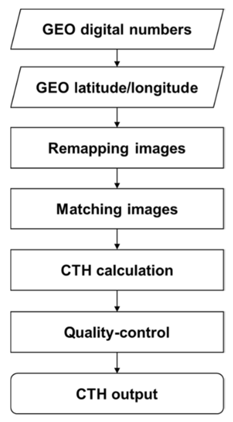
Figure 3.
Example of the image remapping on 3 November 2017 at 05:30 UTC. (a) The FY-2E visible channel image, (b) the Himawari-8 channel 3 image and (c) the Himawari-8 channel 3 image remapped onto FY-2E grid.
Figure 3.
Example of the image remapping on 3 November 2017 at 05:30 UTC. (a) The FY-2E visible channel image, (b) the Himawari-8 channel 3 image and (c) the Himawari-8 channel 3 image remapped onto FY-2E grid.
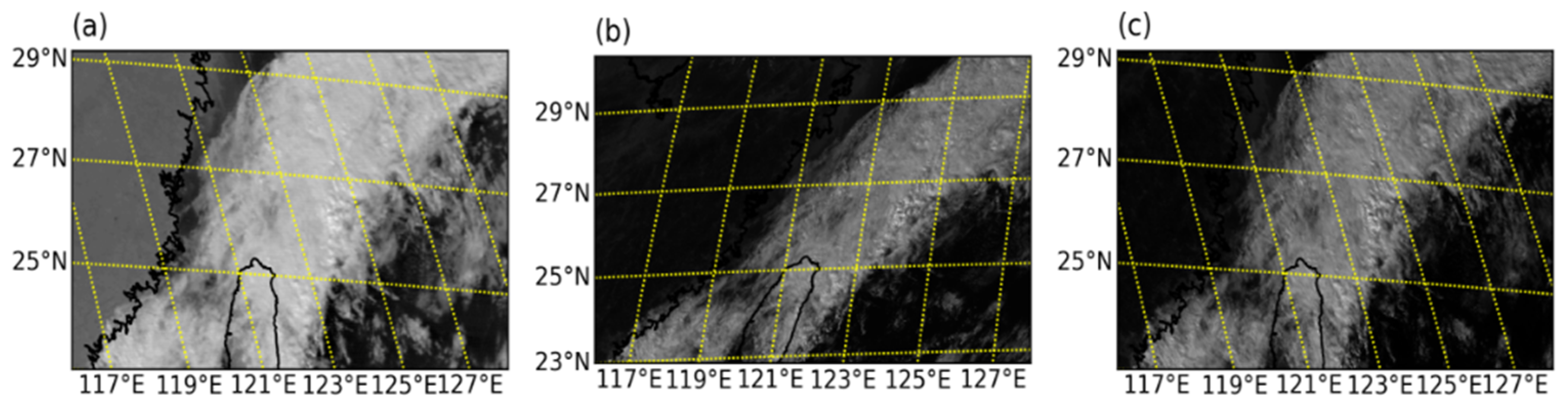
Figure 4.
Example of the image matching on 3 November 2017 at 05:30 UTC. (a) Template image defined in the FY-2E visible (VIS) image. (b) Source image centered on the location of template image selected in the remapped Himawari-8 channel 3 image. (c) Normalized cross correlation matrix obtained by shifting the defined template image by one pixel in the source image.
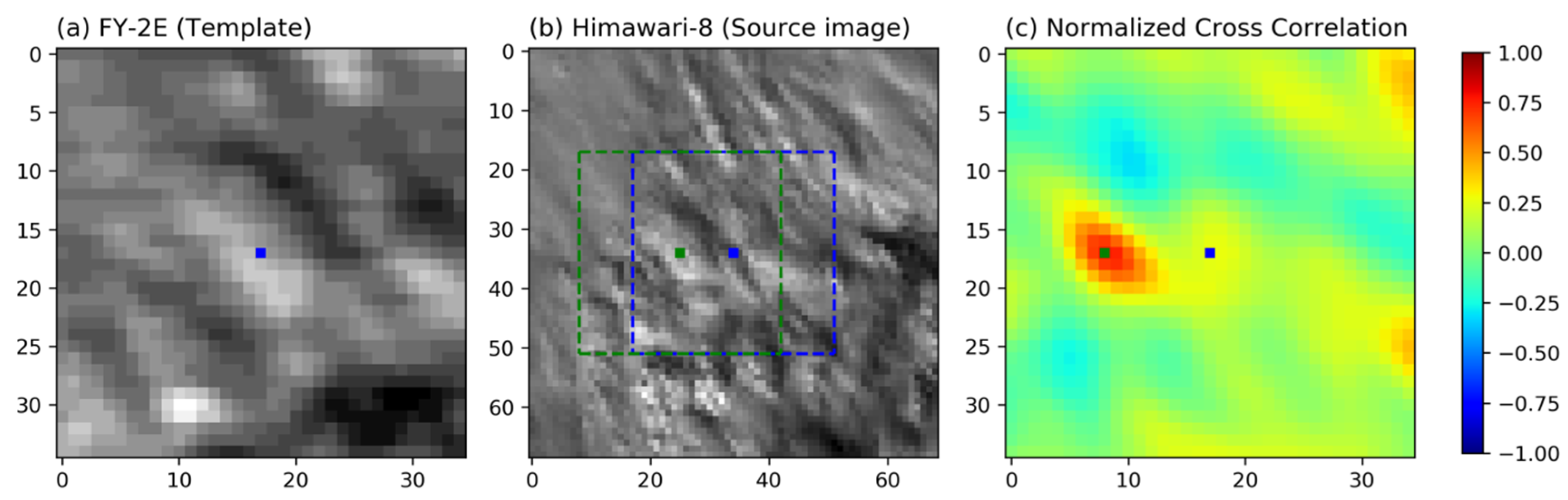
Figure 5.
Example of the scan time correction on 3 November 2017. (a) Normalized cross correlation matrix for the first image matching using remapped Himawari-8 channel 3 image and FY-2E VIS image at 05:30 UTC (same as Figure 4c). (b) Same as (a), but for the second image matching using the consecutive remapped Himawari-8 channel 3 image and FY-2E VIS image (i.e., 05:30 UTC, 05:40 UTC for FY-2E and Himawari-8, respectively). The green and cyan squares in (a) and (b) represent the pixel with maximum NCC. The blue square indicates the center of the template image. (c) Result of the scan time correction. Two pixels with maximum NCC are linearly interpolated at the scan time of FY-2E, as expressed by the red square in (c).
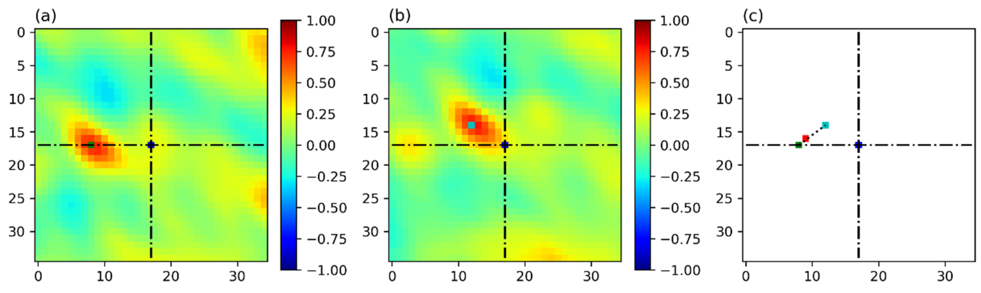
Figure 6.
(a) Schematic diagram and (b) flowchart of the iterative method in the dual-GEO CTH algorithm.
Figure 6.
(a) Schematic diagram and (b) flowchart of the iterative method in the dual-GEO CTH algorithm.
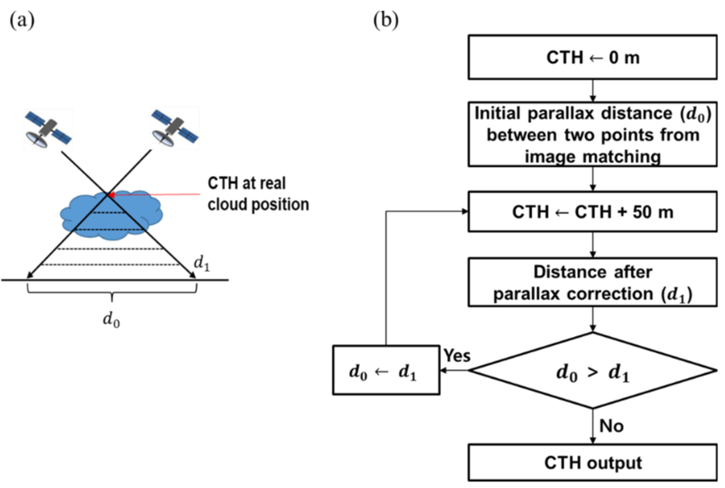
Figure 7.
(a) Dual-GEO CTHs and (b) Himawari-8 CTHs (km) on 8 November 2017 at 05:30 UTC. The grey solid line in (a) and (b) indicates CALIPSO/CloudSat overpass. (c) CALIOP 532 nm total attenuated backscatter (km−1sr−1) and (d) CPR 94 GHz reflectivity (dBZ) along CALIPSO/CloudSat overpass.
Figure 7.
(a) Dual-GEO CTHs and (b) Himawari-8 CTHs (km) on 8 November 2017 at 05:30 UTC. The grey solid line in (a) and (b) indicates CALIPSO/CloudSat overpass. (c) CALIOP 532 nm total attenuated backscatter (km−1sr−1) and (d) CPR 94 GHz reflectivity (dBZ) along CALIPSO/CloudSat overpass.
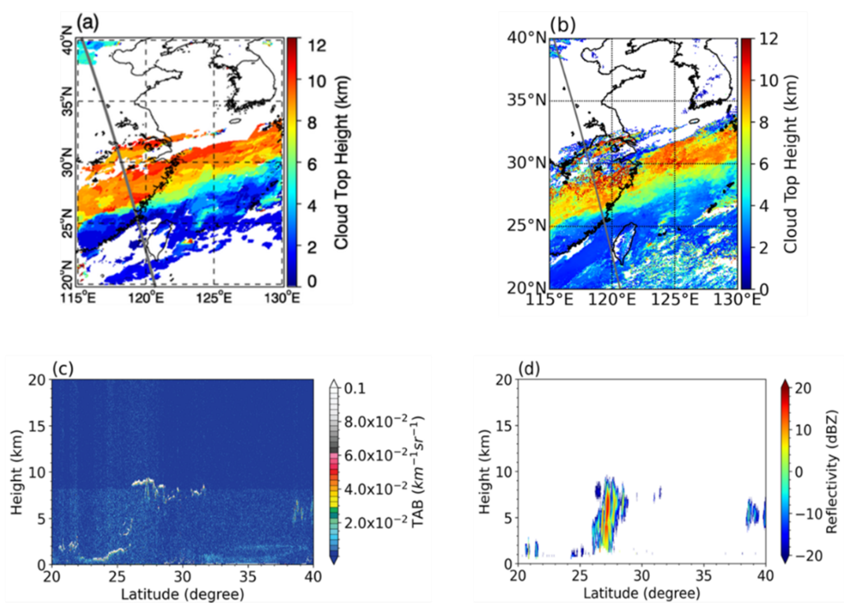
Figure 8.
CTHs (km) retrieved from CALIOP, CPR, Himawari-8, and dual-GEO CTH algorithm along the CALIPSO/CloudSat overpass on 8 November 2017 at 05:30 UTC. CALIOP, CPR, Himawari-8, and dual-GEO CTHs are represented by the blue, red, green, and black circles, respectively.
Figure 8.
CTHs (km) retrieved from CALIOP, CPR, Himawari-8, and dual-GEO CTH algorithm along the CALIPSO/CloudSat overpass on 8 November 2017 at 05:30 UTC. CALIOP, CPR, Himawari-8, and dual-GEO CTHs are represented by the blue, red, green, and black circles, respectively.
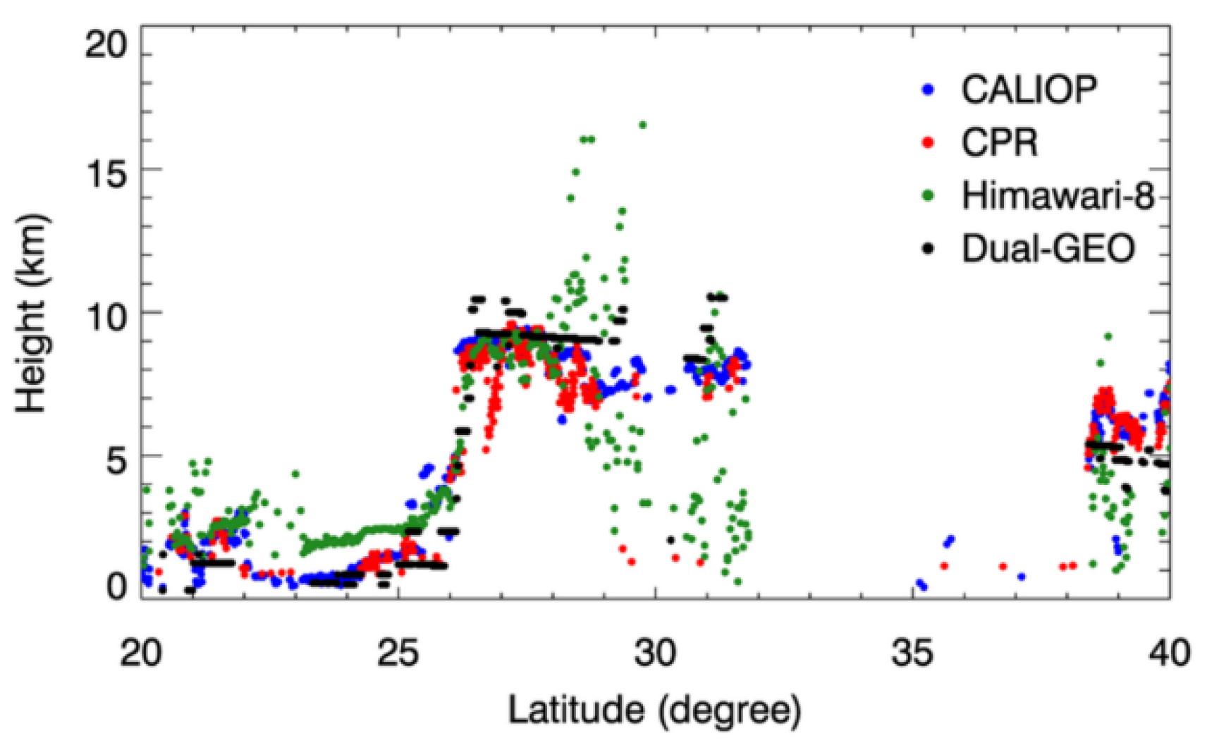
Figure 9.
(a,b) Scatterplots of dual-GEO CTHs and (c,d) Himawari-8 CTHs (km) against CALIOP and CPR CTHs on 8 November 2017 at 05:30 UTC. Red lines in (a–d) indicate linear regression lines.
Figure 9.
(a,b) Scatterplots of dual-GEO CTHs and (c,d) Himawari-8 CTHs (km) against CALIOP and CPR CTHs on 8 November 2017 at 05:30 UTC. Red lines in (a–d) indicate linear regression lines.

Figure 10.
(a) Dual-GEO CTHs and (b) Himawari-8 CTHs (km) on 21 September 2017 at 05:30 UTC. The grey solid line in (a) and (b) indicates CALIPSO/CloudSat overpass. (c) CALIOP 532 nm total attenuated backscatter (km−1sr−1) and (d) CPR 94 GHz reflectivity (dBZ) along CALIPSO/CloudSat overpass. Note that color bar ranges of (a) and (b) are different from those of Figure 7.

Figure 11.
CTHs (km) retrieved from CALIOP, CPR, Himawari-8, and dual-GEO CTH algorithm along the CALIPSO/CloudSat overpass on 21 September 2017 at 05:30 UTC. CALIOP, CPR, Himawari-8, and dual-GEO CTHs are represented by the blue, red, green, and black circles, respectively.
Figure 11.
CTHs (km) retrieved from CALIOP, CPR, Himawari-8, and dual-GEO CTH algorithm along the CALIPSO/CloudSat overpass on 21 September 2017 at 05:30 UTC. CALIOP, CPR, Himawari-8, and dual-GEO CTHs are represented by the blue, red, green, and black circles, respectively.
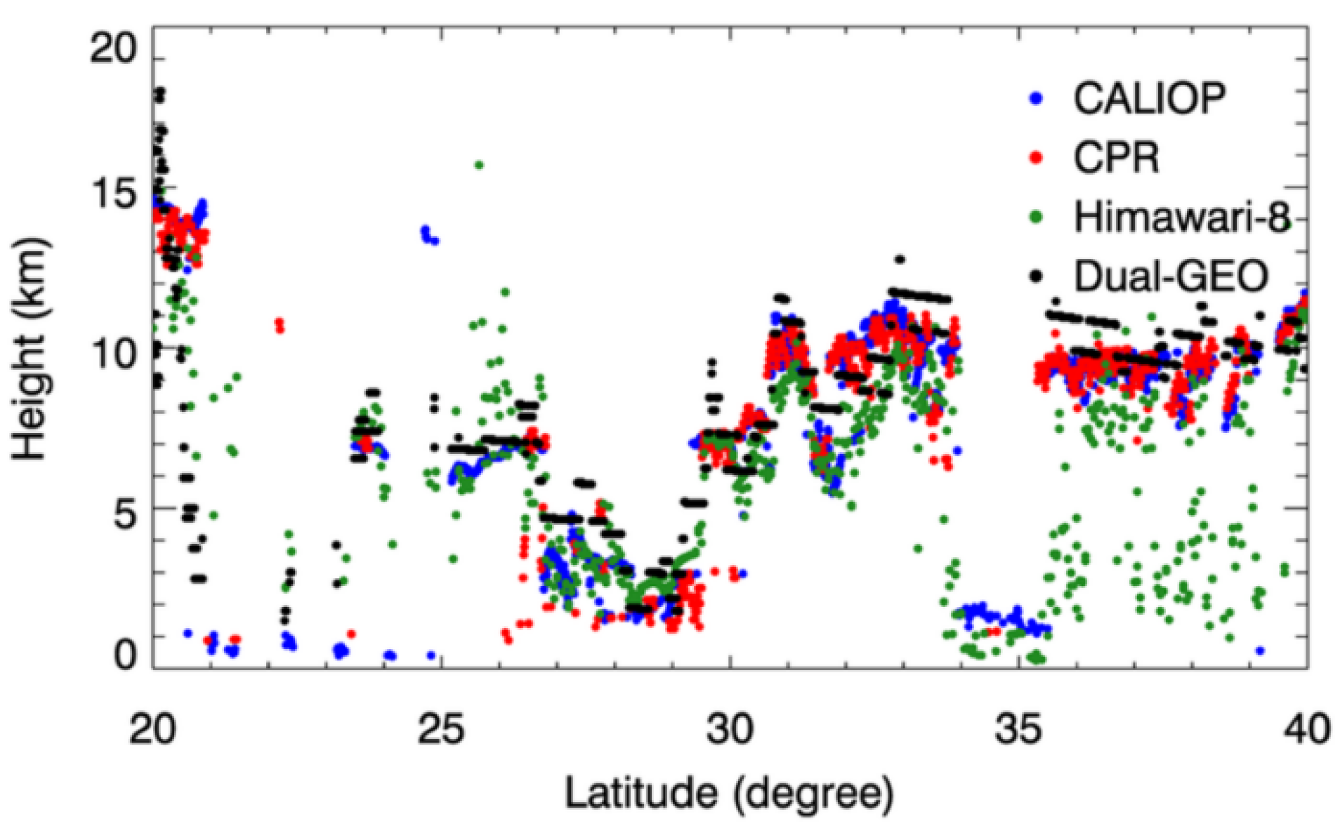
Figure 12.
(a,b) Scatterplots of dual-GEO CTHs and (c,d) Himawari-8 CTHs (km) against CALIOP and CPR CTHs on 21 September 2017 at 05:30 UTC. Red lines in (a–d) indicate linear regression lines.
Figure 12.
(a,b) Scatterplots of dual-GEO CTHs and (c,d) Himawari-8 CTHs (km) against CALIOP and CPR CTHs on 21 September 2017 at 05:30 UTC. Red lines in (a–d) indicate linear regression lines.
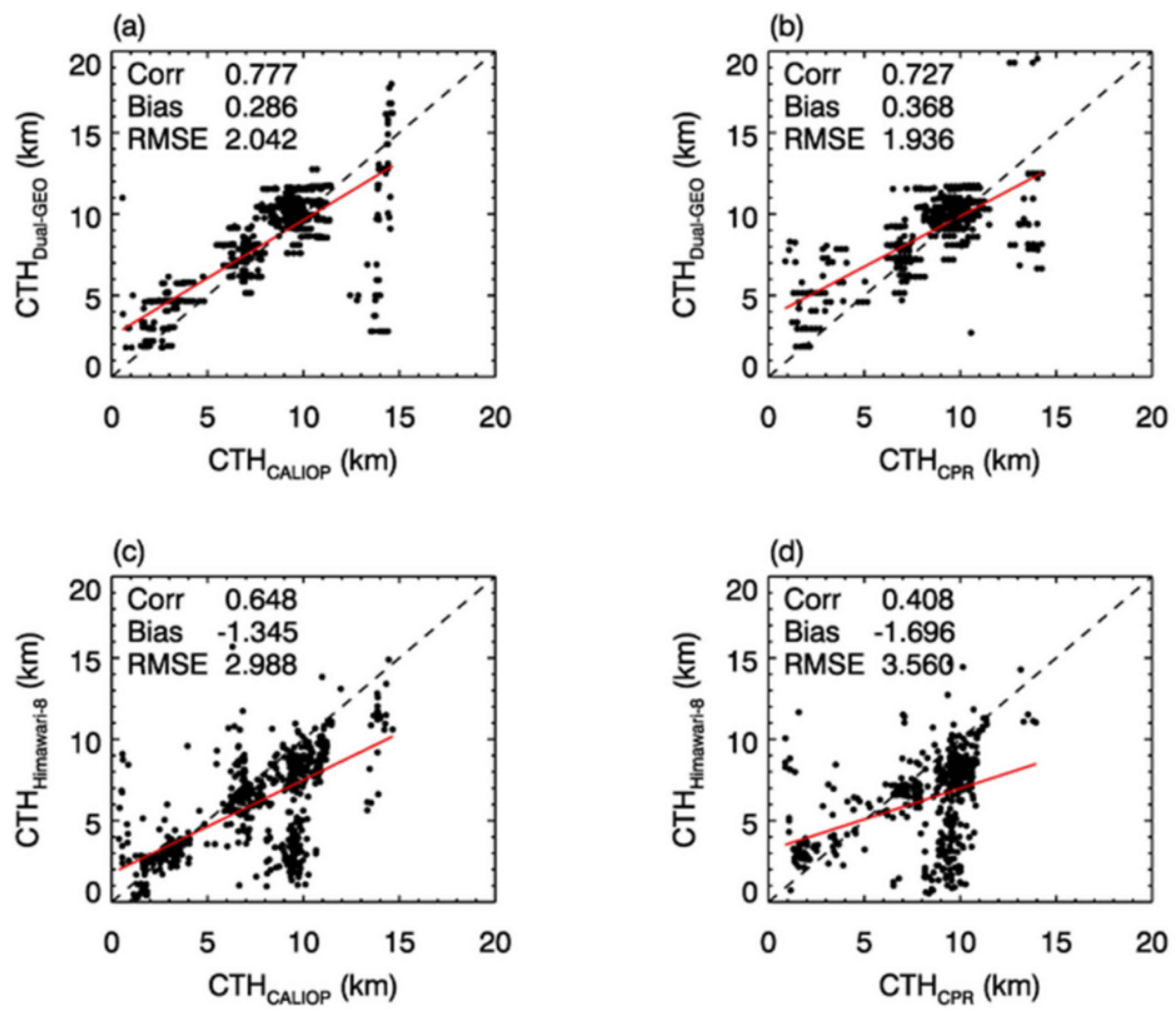
Figure 13.
(a) Dual-GEO CTHs and (b) Himawari-8 CTHs (km) on 3 November 2017 at 05:30 UTC. The grey solid line in (a) and (b) indicates CALIPSO/CloudSat overpass. (c) CALIOP 532 nm total attenuated backscatter (km−1sr−1) and (d) CPR 94 GHz reflectivity (dBZ) along CALIPSO/CloudSat overpass.
Figure 13.
(a) Dual-GEO CTHs and (b) Himawari-8 CTHs (km) on 3 November 2017 at 05:30 UTC. The grey solid line in (a) and (b) indicates CALIPSO/CloudSat overpass. (c) CALIOP 532 nm total attenuated backscatter (km−1sr−1) and (d) CPR 94 GHz reflectivity (dBZ) along CALIPSO/CloudSat overpass.
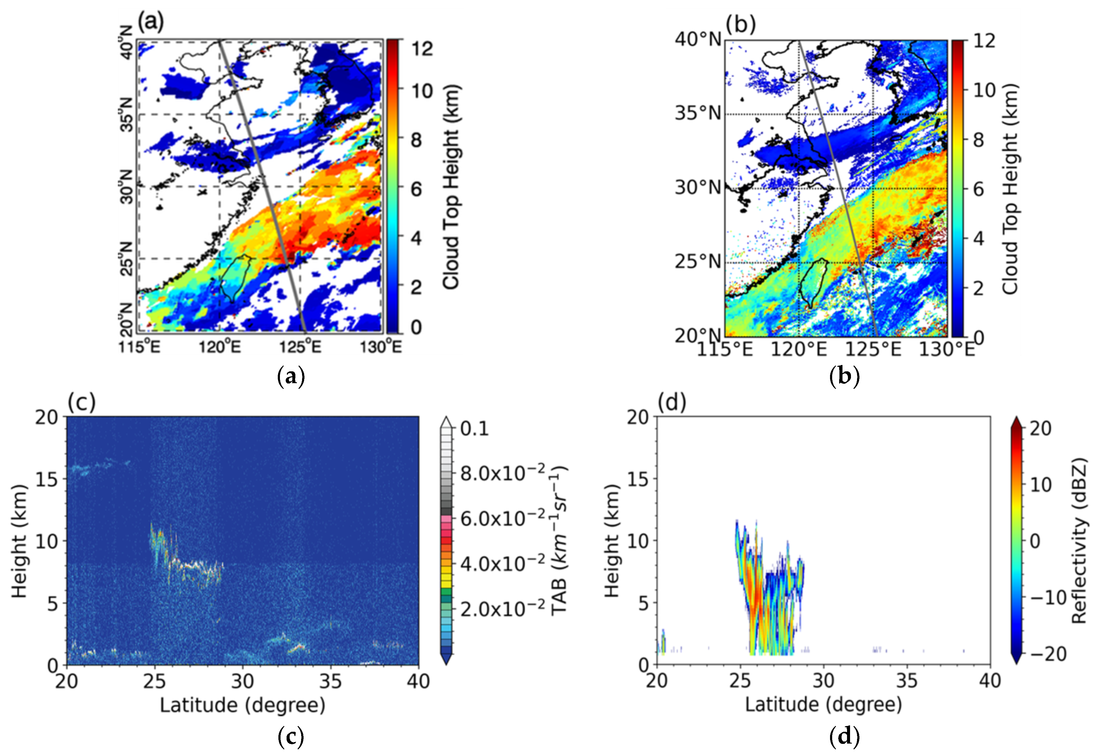
Figure 14.
CTHs (km) retrieved from CALIOP, CPR, Himawari-8, and dual-GEO CTH algorithm along the CALIPSO/CloudSat overpass on 3 November 2017 at 05:30 UTC. CALIOP, CPR, Himawari-8, and dual-GEO CTHs are represented by the blue, red, green, and black circles, respectively.
Figure 14.
CTHs (km) retrieved from CALIOP, CPR, Himawari-8, and dual-GEO CTH algorithm along the CALIPSO/CloudSat overpass on 3 November 2017 at 05:30 UTC. CALIOP, CPR, Himawari-8, and dual-GEO CTHs are represented by the blue, red, green, and black circles, respectively.
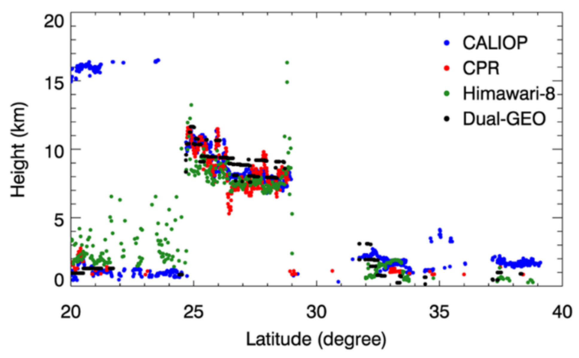
Figure 15.
(a,b) Scatterplots of dual-GEO CTHs and (c,d) Himawari-8 CTHs (km) against CALIOP and CPR CTHs on 3 November 2017 at 05:30 UTC. Red lines in (a–d) indicate linear regression lines.
Figure 15.
(a,b) Scatterplots of dual-GEO CTHs and (c,d) Himawari-8 CTHs (km) against CALIOP and CPR CTHs on 3 November 2017 at 05:30 UTC. Red lines in (a–d) indicate linear regression lines.


Table 1.
Characteristics of the Himawari-8 Advanced Himawari Imager (AHI) and the FengYun (FY)-2E Stretched Visible and Infrared Spin Scan Radiometer (S-VISSR). Channels used in the dual-geostationary (GEO) cloud-top height (CTH) algorithm are shaded in grey.
Table 1.
Characteristics of the Himawari-8 Advanced Himawari Imager (AHI) and the FengYun (FY)-2E Stretched Visible and Infrared Spin Scan Radiometer (S-VISSR). Channels used in the dual-geostationary (GEO) cloud-top height (CTH) algorithm are shaded in grey.
| Channel Number | Channel | AHI Central Wavelength (µm) | Spatial Resolution (km) | S-VISSR Wavelength Range (µm) | Spatial Resolution (km) |
|---|---|---|---|---|---|
| 1 | Visible | 0.47 | 1.0 | ||
| 2 | 0.51 | 1.0 | |||
| 3 | 0.64 | 0.5 | 0.55–0.90 | 1.25 | |
| 4 | Near-Infrared | 0.86 | 1.0 | ||
| 5 | 1.6 | 2.0 | |||
| 6 | 2.3 | 2.0 | |||
| 7 | Infrared | 3.9 | 2.0 | 3.5–4.0 | 5.0 |
| 8 | 6.2 | 2.0 | |||
| 9 | 6.9 | 2.0 | 6.3–7.6 | 5.0 | |
| 10 | 7.3 | 2.0 | |||
| 11 | 8.6 | 2.0 | |||
| 12 | 9.6 | 2.0 | |||
| 13 | 10.4 | 2.0 | 10.3–11.3 | 5.0 | |
| 14 | 11.2 | 2.0 | |||
| 15 | 12.4 | 2.0 | 11.5–12.5 | 5.0 | |
| 16 | 13.3 | 2.0 |
Table 2.
List of products used to validate the dual-GEO CTH algorithm.
| Satellite/Instrument | Product Name | Product Version | Variable Name |
|---|---|---|---|
| CALIPSO 1/CALIOP 2 | CAL_LID_L1 | 4.10 | Total_Attenuated_Backscatter_532 |
| CAL_LID_L2_01kmCLay | 4.20 | Layer_Top_Altitude | |
| CloudSat/CPR 3 | 2B-GEOPROF | 4.0 | CPR_Cloud_Mask |
| Himawari-8/AHI 4 | L2CLP010 | 1.0 | CLTH |
1 CALIPSO: Cloud Aerosol Lidar and Infrared Pathfinder Satellite 2 CALIOP: Cloud Aerosol Lidar with Orthogonal Polarization 3 CPR: Cloud Profiling Radar 4 AHI: Advanced Himawari Imager.
Table 3.
List of parameters used in the dual-GEO CTH algorithm.
| Parameter | Value |
|---|---|
| Normalized cross-correlation (NCC) threshold | 0.5 |
| Template image size | 35 × 35 |
| Source image size | 69 × 69 |
| Maximum allowed horizontal shift | 17 |
| Maximum allowed vertical shift | 17 |
Table 4.
Theoretical accuracy (km) of other satellite combinations in East Asia. Base-to-height ratios of the two satellites are in parentheses.
Table 4.
Theoretical accuracy (km) of other satellite combinations in East Asia. Base-to-height ratios of the two satellites are in parentheses.
| Satellite (longitude) | FY-2E (86.5°E) | FY-2G (104.5°E) | FY-4A (104.7°E) | FY-2F (112.0°E) | GK-2A (128.2°E) | Himawari-8 (140.7°E) |
|---|---|---|---|---|---|---|
| FY-2E (86.5°E) | - | 2.713 (0.369) | 2.683 (0.373) | 1.923 (0.520) | 1.192 (0.839) | 0.932 (1.073) |
| FY-2G (104.5°E) | - | 243.149 (0.004) | 6.49 (0.154) | 2.07 (0.484) | 1.37 (0.732) | |
| FY-4A (104.7°E) | - | 6.67 (0.150) | 1.04 (0.480) | 0.69 (0.728) | ||
| FY-2F (112.0°E) | - | 3.01 (0.332) | 1.71(0.584) | |||
| GK-2A (128.2°E) | - | 1.95 (0.257) | ||||
| Himawari-8 (140.7°E) | - |
© 2020 by the authors. Licensee MDPI, Basel, Switzerland. This article is an open access article distributed under the terms and conditions of the Creative Commons Attribution (CC BY) license (http://creativecommons.org/licenses/by/4.0/).
Share and Cite
MDPI and ACS Style
Lee, J.; Shin, D.-B.; Chung, C.-Y.; Kim, J. A Cloud Top-Height Retrieval Algorithm Using Simultaneous Observations from the Himawari-8 and FY-2E Satellites. Remote Sens. 2020, 12, 1953. https://doi.org/10.3390/rs12121953
AMA Style
Lee J, Shin D-B, Chung C-Y, Kim J. A Cloud Top-Height Retrieval Algorithm Using Simultaneous Observations from the Himawari-8 and FY-2E Satellites. Remote Sensing. 2020; 12(12):1953. https://doi.org/10.3390/rs12121953
Chicago/Turabian StyleLee, Jonghyuk, Dong-Bin Shin, Chu-Yong Chung, and JaeGwan Kim. 2020. "A Cloud Top-Height Retrieval Algorithm Using Simultaneous Observations from the Himawari-8 and FY-2E Satellites" Remote Sensing 12, no. 12: 1953. https://doi.org/10.3390/rs12121953
Note that from the first issue of 2016, this journal uses article numbers instead of page numbers. See further details here.