On the Recursive Joint Position and Attitude Determination in Multi-Antenna GNSS Platforms

Abstract

Global Navigation Satellite Systems’ (GNSS) carrier phase observations are fundamental in the provision of precise navigation for modern applications in intelligent transport systems. Differential precise positioning requires the use of a base station nearby the vehicle location, while attitude determination requires the vehicle to be equipped with a setup of multiple GNSS antennas. In the GNSS context, positioning and attitude determination have been traditionally tackled in a separate manner, thus losing valuable correlated information, and for the latter only in batch form. The main goal of this contribution is to shed some light on the recursive joint estimation of position and attitude in multi-antenna GNSS platforms. We propose a new formulation for the joint positioning and attitude (JPA) determination using quaternion rotations. A Bayesian recursive formulation for JPA is proposed, for which we derive a Kalman filter-like solution. To support the discussion and assess the performance of the new JPA, the proposed methodology is compared to standard approaches with actual data collected from a dynamic scenario under the influence of severe multipath effects.

1. Introduction

As contemporary applications such as driverless cars or autonomous shipping are called to revolutionize intelligent transportation systems (ITS), there is a growing need for the provision of precise and reliable navigation information. Global Navigation Satellite Systems (GNSS) play a fundamental role, becoming the main information supplier of positioning, navigation, and timing (PNT) data. While standard GNSS techniques—based on code observations— provide a decent performance for many applications, they do not comply with the far more stringent precision requirements of modern safety-critical scenarios. That is the reason why the transition to carrier phase-based techniques is required to reach precise navigation. Indeed, carrier phase observations present noise levels two orders of magnitude lower than their code counterpart. However, carrier phase observations are ambiguous, since only their fractional part is measured by the receiver [1]. The unknown number of integer cycles between satellite and receiver, so-called ambiguities, must be estimated to enable high-precision navigation. The ambiguities’ estimation process is widely known as ambiguity resolution (AR) [2,3,4,5], which in turn results in a challenging estimation procedure.

From the use of the carrier phase for precise positioning, two localization techniques are distinguished: (i) precise point positioning (PPP) ([6], Ch. 25) and (ii) real-time kinematics (RTK) ([6], Ch. 26). The former exploit GNSS precise corrections for atmospheric effects, satellite orbits, clocks, and antenna biases. This requires the connection to a global network of stations providing such corrections, which might not be available in real-time (i.e., several days are needed for final ephemeris products), then limiting its use in certain applications. In addition, PPP is also constrained by a long convergence time, ranging from five to 20 min [7]. On the other hand, RTK is a relative positioning procedure where the location of a vehicle is determined with respect to (w.r.t.) a stationary or virtual base station of known coordinates, achieving centimeter-level precision. Although limited by the need for proximal base stations and a communication channel, high-precision positioning can be obtained almost immediately, making RTK more appealing than PPP for certain real-time applications. This work focuses on the RTK model to address the positioning problem.

Another well-known application of GNSS carrier phase measurements relates to attitude determination. Attitude determination is the process of estimating the orientation of a moving rigid body w.r.t. its environment. In a multi-antenna GNSS system, one seeks to estimate the rotation, which relates the baseline vectors joining each pair of antenna positions across two frames of interest. Despite GNSS providing substantially higher precision than other attitude determination systems, its implementation poses some constraints. On the one hand, at least three non-coplanar GNSS antennas need to be installed and their relative positions accurately surveyed in the vehicle local frame. On the other hand, attitude precision is inversely proportional to the separation between antennas, making this system impractical for small vehicles (i.e., such as unmanned aerial vehicles). An overview of the formulation for GNSS-based attitude determination was introduced in [8], showing the relationship between carrier phase AR and the corresponding rotation matrix. In addition, the work in [8] discussed multi-epoch orientation solving and suggested a batch least-squares (LS) solution, which gathers GNSS observations along some period of time. This solution is however generally incompatible with real-time applications. The concept of multivariate-constrained Least-squares AMBiguity Decorrelation Adjustment (MC-LAMBDA) for GNSS carrier phase-based attitude determination was introduced in [1,9,10], becoming the most popular and effective attitude determination method.

Traditionally, the positioning and attitude determination problems are considered as two independent processes. Even when integrated as part of the same filtering solution [11,12,13,14,15], the cross-correlation between the positioning- and attitude-related observations is disregarded. However, this information results in being very useful, and it strengthens the overall observation model. Despite its importance in many engineering fields, there are few contributions discussing the topic and a lack of understanding of the concept of joint position and attitude (JPA) based on the exploitation of GNSS carrier phase observables, which in turn is the central interest of this work. There are several important missing points related to JPA, which to the best of the authors’ knowledge, have never been explored and constitute the contribution of this article:

(1)

The GNSS carrier phase-based positioning and attitude models are revisited, and the connection to the JPA problem is formalized.

(2)

Application of Lie theory principles to the GNSS-based attitude problem (and consequently, also the JPA). Thus, the attitude is parametrized with the unit-quaternion, and a recursive solution based on an error state Kalman filter (ESKF) is formulated.

(3)

The performance of the proposed recursive solution for the JPA problem is addressed on a realistic signal-degraded scenario, and the comparison w.r.t separately solving the positioning and attitude problems (i.e., the standard solution) is analyzed.

The rest of the paper is organized as follows. Section 2 presents the notation employed throughout the paper, the coordinate frames involved in the estimation process, and the state definitions of the JPA. Then, Section 3 discusses the carrier phase-based positioning and attitude models. Section 4 relates the GNSS observations models to the JPA problem, and the Kalman Filter-like recursive solution is presented. The experimentation and posterior discussion are presented in Section 5. Finally, Section 7 concludes the paper with an outlook and discussion of future work directions.

2. Notation and Definitions

2.1. Notation

Italics indicate a scalar quantity, as in c; lower case boldface indicates a column vector quantity, as in $\mathsf{a}$; upper case boldface indicates a matrix quantity, as in $\mathsf{A}$. The matrix/vector transpose is indicated by a superscript ${(·)}^{\top }$ as in ${\mathsf{A}}^{\top }$. $\left[\mathsf{A},\mathsf{B}\right]$ and $\left[\genfrac{}{}{0pt}{}{\mathsf{A}}{\mathsf{B}}\right]$ denote the matrix resulting from the horizontal and the vertical concatenation of $\mathsf{A}$ and $\mathsf{B}$, respectively. ${\mathsf{I}}_M$ is the identity matrix of dimension M. ${\mathbf{1}}_{M,N}$ is an $M\times N$-dimensional matrix with all components equal to one. ${\mathbf{0}}_{M,N}$ is an $M\times N$-dimensional matrix with all components equal to zero. $\parallel ·\parallel$ denotes a Euclidean norm, and ${\parallel \mathsf{b}\parallel }_A^2={\mathsf{b}}^{\top }{\mathsf{A}}^{-1}\mathsf{b}$ is the weighted inner norm. $E(·)$ and $D(·)$ represent the expectation and dispersion operator respectively. $\mathrm{vec}(·)$ is the operator that stacks the columns of a matrix $\mathsf{A}$ into a single vector. $\mathsf{A}=\mathrm{diag}(·)$ indicates a diagonal matrix whose entries in the diagonal are given by $(·$). The Kronecker product is denoted with ⊗. The quaternion multiplication is denoted by ∘.

2.2. Coordinate Frames

In general, a navigation system involves the determination of the position, velocity, and attitude of a moving (rigid) body. The kinematic quantities generally involve two coordinate frames: (i) the frame whose motion is described, the body or vehicle frame $\mathcal{B}$, and (ii) the frame with respect to which that motion is, denoted as the global or inertial frame $\mathcal{G}$. For the problem at hand, the body frame is defined such that the X-, Y-, and Z-axes are aligned with the right, forward, and up directions of the vehicle, respectively, while the global frame corresponds to the Earth-centered Earth-fixed (ECEF) frame. A pictorial example of the aforementioned frames is given in Figure 1 (left). The left subscript on a vector indicates the frame in which that vector is expressed, while the right subscript refers to a specific position (i.e., any of the onboard vehicle antennas or the base station).

In multi-antenna GNSS platforms, one generally considers the position of the master antenna as the center of the body frame and the unknown position to be determined ${}_{\mathcal{G}}\mathsf{p}\triangleq {}_{\mathcal{G}}{\mathsf{p}}_m$, while the positions of the remaining N slave antennas ${}_{\mathcal{G}}{\mathsf{p}}_j$ (with $j=1,\cdots ,N$) are referred to the former with the respective baseline vectors. For instance, the position in the body frame for the jth slave antenna is as:

$${}_{\mathcal{B}}{\mathsf{p}}_j={}_{\mathcal{B}}{\mathsf{p}}_m+{}_{\mathcal{B}}{\mathsf{b}}_{j,m}$$

(1)

where the baseline vector ${}_{\mathcal{B}}{\mathsf{b}}_{j,m}$ in the body frame is known a priori. Similarly, the position in the global frame for the jth antenna can be easily formulated upon the knowledge of the master position and the rotation relating the body and global frames.

$$\begin{array}{c}\hfill {}_{\mathcal{G}}{\mathsf{p}}_j={}_{\mathcal{G}}{\mathsf{p}}_m+\mathsf{R}{}_{\mathcal{B}}{\mathsf{b}}_{j,m}={}_{\mathcal{G}}{\mathsf{p}}_m+\mathsf{q}\circ {}_{\mathcal{B}}{\mathsf{b}}_{j,m}\circ {\mathsf{q}}^{*}\end{array}$$

(2)

where $\mathsf{R}\in \mathcal{SO}\left(3\right)$ and $\mathsf{q}\in {\mathcal{S}}^3$ are the rotation matrix and unit-quaternion to represent the body-to-global rotation. The quaternion is written as $\mathsf{q}={[cos(\varphi /2),\mathsf{e}sin(\varphi /2)]}^{\top }$ with $\varphi$ a rotation angle and $\mathsf{e}$ a unit rotation axis. The quaternion rotation follows the Hamilton convention (real part first, right handedness). Henceforth, either $\mathsf{R}{}_{\mathcal{B}}\mathsf{u}$ or $\mathsf{q}\circ {}_{\mathcal{B}}\mathsf{u}\circ {\mathsf{q}}^{*}$ are used indistinctly for expressing the body-to-global rotation of a generic vector ${}_{\mathcal{B}}\mathsf{u}$. However, since rotation matrices result in difficult renormalization and computational inefficiency, its use on recursive attitude determination is often discouraged [16,17,18]. Instead, this work focuses on the unit quaternion parametrization for attitude estimation. Additional details on the quaternion group and algebra are provided in Appendix A.

2.3. State Definitions

The proposed JPA problem relates to the estimation of the vehicle kinematics: position ${}_{\mathcal{G}}\mathsf{p}$, velocity ${}_{\mathcal{G}}\mathsf{v}$, and attitude $\mathsf{q}$, as well as the GNSS integer ambiguities $\mathsf{a}$ for the $n+1$ tracked satellites across the onboard and base station antennas, as later defined in Section 3. The state estimate $\mathsf{x}$ is expressed as a discrete-time state-space model, described at a given time t as:

$${\mathsf{x}}_{\mathrm{JPA}}\triangleq \mathsf{x}={\left[\begin{array}{c}{}_{\mathcal{G}}{\mathsf{p}}^{\top },{}_{\mathcal{G}}{\mathsf{v}}^{\top },{\mathsf{q}}^{\top },{\mathsf{a}}^{\top }\end{array}\right]}^{\top },{}_{\mathcal{G}}\mathsf{p},{}_{\mathcal{G}}\mathsf{v}\in {\mathbb{R}}^3,\mathsf{q}\in {\mathcal{S}}^3,\mathsf{a}\in {\mathbb{Z}}^{n\times (N+1)}.$$

(3)

Optionally, the state vector could be augmented to account for the biases of an inertial sensor, whenever that navigation modality is fused along with GNSS. The state defined in (3) is often applied to describe the motion of vehicles following a constant-velocity non-turning movement [19,20], e.g., automobiles, vessels, or aeroplanes moving in a straight line. To describe a wider range of motions, (3) could be extended with the acceleration and angular rate of the vehicle, or an interacting multiple model (IMM) estimator could be applied [21,22].

Preserving the quaternion unit norm constraint is a challenging task, for which Lie theory provides useful algebraic tools whose application in navigation problems is increasingly used [23,24,25]. While the state $\mathsf{x}$ lives in a manifold, its perturbations $\delta \mathsf{x}$ belong to the tangent space of the manifold. The error state Kalman filter (ESKF) allows exploiting the Lie algebra by defining the “true” (unknown) state as the group composition of the total-state $\widehat{\mathsf{x}}$ and the error-state $\delta \mathsf{x}$ as $\mathsf{x}=\widehat{\mathsf{x}}\oplus \delta \mathsf{x}$ [26,27,28]. At time t, the error state is described by:

$$\delta \mathsf{x}={\left[\delta {\mathsf{p}}^{\top },\delta {\mathsf{v}}^{\top },\delta {\theta }^{\top },\delta {\mathsf{a}}^{\top }\right]}^{\top },\delta \mathsf{p},\delta \mathsf{p},\delta \theta \in {\mathbb{R}}^3,\delta \mathsf{a}\in {\mathbb{R}}^{n\times (N+1)},$$

(4)

where the rotation vector $\delta \theta$ can be identified with its associated quaternion $\delta \mathsf{q}$ as follows:

$$\delta \theta \in {\mathbb{R}}^3\stackrel{{(·)}^{\wedge }}{\mapsto }\mathsf{e}\varphi \in {\mathfrak{s}}^3\stackrel{exp(·)}{\mapsto }\delta \mathsf{q}\in {\mathcal{S}}^3.$$

(5)

First, the rotation vector in the Euclidean space $\delta \theta \in {\mathsf{R}}^3$ is related to the Lie algebra $\mathsf{e}\varphi \in {\mathfrak{s}}^3$ through the isomorphism ${(·)}^{\wedge }:{\mathbb{R}}^3\mapsto {\mathfrak{s}}^3$. Then, the Lie algebra is identified with the ${\mathcal{S}}^3$ manifold via exponential mapping $\delta \mathsf{q}=exp\left(\mathsf{e}\varphi \right)={[cos(\varphi /2),\mathsf{e}sin(\varphi /2)]}^{\top }$. Finally, the composition of the total quaternion $\widehat{\mathsf{q}}$ with the error quaternion $\delta \mathsf{q}$ is given by:

$$\mathsf{q}=\widehat{\mathsf{q}}\circ \delta \mathsf{q}$$

(6)

The reader interested in the basics of Lie theory may refer to [29,30] or to a recent selection of these principles in relation to robotics in [31].

3. GNSS Carrier Phase-Based Positioning and Attitude Observation Models

Let us consider $n+1$ GNSS satellites simultaneously tracked (single frequency) at one antenna (i.e., if considering $N+1$ antennas at the vehicle, the observation model remains the same for each antenna) installed on a vehicle and at a base station of known coordinates. At a particular time, the code and phase observables for the ith satellite at the jth antenna (either onboard or base) are:

$$\begin{array}{cc}\hfill {\rho }_j^i& =\parallel {}_{\mathcal{G}}{\mathsf{p}}^i-{}_{\mathcal{G}}{\mathsf{p}}_j\parallel +I^i+T^i+c\left(d{t}_j-d{t}^i\right)+{\epsilon }_j^i,\hfill \\ \hfill {\mathsf{\Phi }}_j^i& =\parallel {}_{\mathcal{G}}{\mathsf{p}}^i-{}_{\mathcal{G}}{\mathsf{p}}_j\parallel -I^i+T^i+c\left(d{t}_j-d{t}^i\right)+\lambda N_j^i+{ϵ}_j^i,\hfill \end{array}$$

(7)

where:

• $\rho ,\mathsf{\Phi }$ are the code and phase observations (m),
• ${}_{\mathcal{G}}{\mathsf{p}}^i,{}_{\mathcal{G}}{\mathsf{p}}_j$ are the positions of the ith satellite and the jth antenna in the global frame,
• $I^i$ is the ionospheric error (m),
• $T^i$ is the tropospheric error (m),
• c is the speed of light ($299792458\mathrm{m}/\mathrm{s}$),
• $d{t}^i,d{t}_j$ are the satellite and receiver clock offsets (s),
• $\lambda$ is the carrier phase wavelength (m),
• $N^i$ is the unknown number of cycles (i.e., in general being a real parameter due to the unknown initial phase at both the satellite and receiver antenna),
• ${\epsilon }^i,{ϵ}^i$ are the remaining noise/unmodeled errors for code and phase observations, respectively.

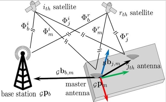
Due to the influence of imprecise ephemeris and atmospheric-related errors, high precision cannot be achieved directly exploiting the observations on (7). Instead, the double-difference combination of observations is fundamental to enable precise positioning and attitude determination, as discussed next. For the remainder of the section, superscripts refer to a particular satellite (r for the pivot and $i=1,\cdots ,n$ for the others), while subscripts denote a particular receiving antenna (m for master antenna, $j=1,\cdots ,N$ for the slave antennas, and b for the base station), as illustrated in Figure 2.

3.1. RTK Positioning Model

RTK is a differential positioning procedure, for which the unknown position of a GNSS antenna is determined w.r.t. a stationary station of known coordinates [32]. To achieve centimeter-level precision positioning, the use of observation double-differencing and integer AR (IAR) is required (details in Section 3.2). Double-difference is the combination formed between two satellites and two receivers to eliminate or minimize nuisance parameters (i.e., atmospheric propagation delays, clock offsets, relativistic effects, etc.) from the involved observables. In the positioning model, the particular double-difference (DD) code and phase measurements (i.e., for the ith satellite, w.r.t. the base b and pivot satellite r, at the master antenna m) are given by:

$$\begin{array}{cc}\hfill DD{\rho }_{b,m}^{i,r}& ={\rho }_b^i-{\rho }_m^i-\left({\rho }_b^r-{\rho }_m^r\right),\hfill \\ \hfill DD{\mathsf{\Phi }}_{b,m}^{i,r}& ={\mathsf{\Phi }}_b^i-{\mathsf{\Phi }}_m^i-\left({\mathsf{\Phi }}_b^r-{\mathsf{\Phi }}_m^r\right),\hfill \end{array}$$

(8)

and the set of positioning DD observations are gathered in the vector ${\mathsf{y}}_{\mathrm{pos}}\in {\mathbb{R}}^{2n}$,

$${\mathsf{y}}_{\mathrm{pos}}\triangleq {\mathsf{y}}_{b,m}={\left[\underset{{\mathsf{DD}{\mathsf{\Phi }}_{b,m}^{1:n,r}}^{\top }}{\underbrace{{DD\mathsf{\Phi }}_{b,m}^{1,r},\cdots ,{DD\mathsf{\Phi }}_{b,m}^{n,r}}},\underset{{\mathsf{DD}{\rho }_{b,m}^{1:n,r}}^{\top }}{\underbrace{{DD\rho }_{b,m}^{1,r},\cdots ,{DD\rho }_{b,m}^{n,r}}}\right]}^{\top }$$

(9)

where the notation ${(·)}_{b,m}^{i,r}$ refers to the DD observation conformed by the base station and master antennas, pivot, and ith satellite and ${(·)}_{b,m}^{1:n,r}$ is the corresponding n-dimensional vector of DD observations. The resulting positioning observation model is generally expressed in its linearized form as:

$$\begin{array}{cc}\hfill {\mathsf{y}}_{\mathrm{pos}}& =\left[\begin{array}{cc}\mathsf{G}& \lambda {\mathsf{I}}_n\\ \mathsf{G}& {\mathbf{0}}_n\end{array}\right]{\mathsf{x}}_{\mathrm{pos}}+{\mathsf{n}}_{\mathrm{pos}}=\underset{{\mathsf{H}}_{\mathrm{pos}}}{\underbrace{\left[\begin{array}{cc}\mathsf{B}& \mathsf{A}\end{array}\right]}}{\mathsf{x}}_{\mathrm{pos}}+{\mathsf{n}}_{\mathrm{pos}},\hfill \end{array}$$

(10)

where $\lambda$ is the carrier wavelength, ${\mathsf{x}}_{\mathrm{pos}}^{\top }=[{}_{\mathcal{G}}{\mathsf{b}}_{b,m}^{\top },{\mathsf{a}}_{\mathrm{pos}}^{\top }]$, ${\mathsf{a}}_{\mathrm{pos}}\in {\mathbb{Z}}^n$ is the vector of ambiguities, and ${}_{\mathcal{G}}{\mathsf{b}}_{b,m}\in {\mathbb{R}}^3$ is the baseline vector between the master and base station positions. ${\mathsf{n}}_{\mathrm{pos}}$ is a zero-mean noise term with covariance ${\mathsf{Q}}_{{\mathsf{y}}_{\mathrm{pos}}}$. The so-called design matrices are:

$$\begin{array}{cc}\hfill & \mathsf{A}=\left[\begin{array}{c}\lambda {\mathsf{I}}_n\\ {\mathbf{0}}_n\end{array}\right],\mathsf{B}=\left[\begin{array}{c}\mathsf{G}\\ \mathsf{G}\end{array}\right],\mathsf{G}=\left[\begin{array}{c}-{\left({\mathsf{u}}^1-{\mathsf{u}}^r\right)}^{\top }\\ ⋮\\ -{\left({\mathsf{u}}^n-{\mathsf{u}}^r\right)}^{\top }\end{array}\right],\hfill \end{array}$$

(11)

where $\mathsf{G}$ is the geometry matrix composed by the satellite steering line-of-sight vectors w.r.t. the base antenna ${\mathsf{u}}^i=\frac{{}_{\mathcal{G}}{\mathsf{p}}^i-{}_{\mathcal{G}}{\mathsf{p}}_b}{∥{}_{\mathcal{G}}{\mathsf{p}}^i-{}_{\mathcal{G}}{\mathsf{p}}_b∥}$ [6]. Re-arranging some terms in (10), the positioning model can be cast as:

$$\begin{array}{cc}\hfill E\left({\mathsf{y}}_{\mathrm{pos}}\right)& =\mathsf{A}{\mathsf{a}}_{\mathrm{pos}}+\mathsf{B}{}_{\mathcal{G}}{\mathsf{b}}_{b,m},D\left({\mathsf{y}}_{\mathrm{pos}}\right)={\mathsf{Q}}_{{\mathsf{y}}_{\mathrm{pos}}}.\hfill \end{array}$$

(12)

Resolving the baseline ${}_{\mathcal{G}}{\mathsf{b}}_{b,m}$ between the base station and the master antenna grants knowing the position of the master antenna as:

$${}_{\mathcal{G}}{\mathsf{p}}_m={}_{\mathcal{G}}{\mathsf{p}}_b-{}_{\mathcal{G}}{\mathsf{b}}_{b,m}.$$

(13)

Notice that in contrast to (7), where the unknown ambiguities $N_m^i\in \mathbb{R}$, because of double-differencing, we now have integer ambiguities ${\mathsf{a}}_{\mathrm{pos}}\in {\mathbb{Z}}^n$. That is, to solve the estimation problem defined by the linearized Gaussian observation model (10), we have to resort to AR techniques (see Section 3.2), which applied to the previous equations, define the single-antenna RTK solution.

3.2. Integer Ambiguity Resolution for Positioning

The system of observation equations in (10) leads to an optimization problem with mixed real and integer parameter estimation. For simplicity, let us rename the variables for the positioning model in (10), i.e., $\mathsf{y}\triangleq {\mathsf{y}}_{\mathrm{pos}}$, ${\mathsf{Q}}_{\mathsf{y}}\triangleq {\mathsf{Q}}_{{\mathsf{y}}_{\mathrm{pos}}}$, $\mathsf{a}\triangleq {\mathsf{a}}_{\mathrm{pos}}$, and $\mathsf{b}\triangleq {}_{\mathcal{G}}{\mathsf{b}}_{b,m}$. Thus, we want to solve:

$$\{\mathsf{a},\mathsf{b}\}=arg\underset{\mathsf{b}\in {\mathbb{R}}^3,\mathsf{a}\in {\mathbb{Z}}^n}{min}{∥\mathsf{y}-\mathsf{A}\mathsf{a}-\mathsf{B}\mathsf{b}∥}_{{\mathsf{Q}}_{\mathsf{y}}}^2.$$

(14)

Due to the integer nature of $\mathsf{a}$, a closed-form solution to (14) is not known. Instead, the work in [33] proposed the decomposition of the quadratic objective function (14) into the sum of three successive LS problems,

$$\begin{array}{cc}\hfill & \underset{\begin{array}{c}\mathsf{b}\in {\mathbb{R}}^3\\ \mathsf{a}\in {\mathbb{Z}}^n\end{array}}{min}{∥\mathsf{y}-\mathsf{A}\mathsf{a}-\mathsf{B}\mathsf{b}∥}_{{\mathsf{Q}}_{\mathsf{y}}}^2=\underset{\begin{array}{c}\widehat{\mathsf{b}}\in {\mathbb{R}}^3\\ \widehat{\mathsf{a}}\in {\mathbb{R}}^n\end{array}}{min}{∥\mathsf{y}-\mathsf{A}\widehat{\mathsf{a}}-\mathsf{B}\widehat{\mathsf{b}}∥}_{{\mathsf{Q}}_{\mathsf{y}}}^2+\underset{\mathsf{a}\in {\mathbb{Z}}^n}{min}{∥\widehat{\mathsf{a}}-\mathsf{a}∥}_{{\mathsf{Q}}_{\widehat{\mathsf{a}}}}^2+\underset{\mathsf{b}\in {\mathbb{R}}^3}{min}{∥\widehat{\mathsf{b}}|\mathsf{a}-\mathsf{b}∥}_{{\mathsf{Q}}_{\widehat{\mathsf{b}}|\mathsf{a}}}^2,\hfill \end{array}$$

(15)

where the first term on the right-hand side is the so-called float solution, $min{∥\mathsf{y}-\mathsf{A}\widehat{\mathsf{a}}-\mathsf{B}\widehat{\mathsf{b}}∥}_{{\mathsf{Q}}_{\mathsf{y}}}^2$, a weighted LS (WLS) disregarding the integer constraints on $\mathsf{a}$, that is $\widehat{\mathsf{a}}$ is the real or float estimation of the ambiguities.

The second term, $min{∥\widehat{\mathsf{a}}-\mathsf{a}∥}_{{\mathsf{Q}}_{\widehat{a}}}^2$, corresponds to the integer LS (ILS), for which the integer ambiguities $\mathsf{a}$ are found based on the estimated float ambiguities $\widehat{\mathsf{a}}$ and their associated covariance ${\mathsf{Q}}_{\widehat{\mathsf{a}}}$. The framework for integer aperture (IA) estimation comprises solving the aforementioned ILS problem and the validation of the obtained solution. A profound discussion on estimators for integer estimation problems can be found in ([6], Chap. 23). Finally, the third term $min{∥\widehat{\mathsf{b}}|\mathsf{a}-\mathsf{b}∥}_{{\mathsf{Q}}_{\widehat{\mathsf{b}}|\mathsf{a}}}^2$ is the fix solution. It consists of enhancing the localization estimates upon the estimated integer ambiguities, resolved upon a WLS estimate:

$$\mathsf{b}=\widehat{\mathsf{b}}-{\mathsf{Q}}_{\widehat{\mathsf{b}},\widehat{\mathsf{a}}}{\mathsf{Q}}_{\widehat{\mathsf{a}}}^{-1}\left(\widehat{\mathsf{a}}-\mathsf{a}\right)$$

(16)

where ${\mathsf{Q}}_{\widehat{\mathsf{b}},\widehat{\mathsf{a}}}$ refers to the cross-covariance matrix between the float estimates for position and ambiguities. A relevant remark is that, whenever the estimated integer ambiguities do not match the true ones, the fixed solution will be biased. The precision of the solution improves only when the correct ambiguities are estimated.

3.3. A Comment on Multi-Antenna DD Observations and Processing

Notice that the previous standard RTK solution was formulated for a single master antenna. One could think that having multiple ($N+1$) antennas, i.e., N times more observations, would certainly improve the overall estimation. The trivial solution is to reformulate the model in (10) taking into account an $N+1$ (i.e., master + N slave antennas) multi-antenna GNSS platform. Notice that in that case, we have $N+1$ unknown baseline vectors between the base and the different antennas to be estimated alongside the $n\times (N+1)$ integer ambiguities. The multi-antenna (MA) measurement vector is then:

$$\begin{array}{cc}\hfill & {\mathsf{y}}_{\mathrm{pos},\mathrm{MA}}={\left[{\mathsf{y}}_{b,m}^{\top },{\mathsf{y}}_{b,1}^{\top },\cdots ,{\mathsf{y}}_{b,N}^{\top }\right]}^{\top }\in {\mathbb{R}}^{2n\times (N+1)},\hfill \end{array}$$

(17)

where ${\mathsf{y}}_{b,m}$ corresponds to (9) and the DD observations formed by the base station and the slave antennas ${\mathsf{y}}_{b,j},j=1,\cdots ,N$, can be built as in (8) changing the index m by j. Thus, the corresponding linearized MA observation model is the concatenation of the single-antenna model (10) as:

$$\begin{array}{cc}\hfill {\mathsf{y}}_{\mathrm{pos},\mathrm{MA}}& ={\mathsf{I}}_{N+1}\otimes {\mathsf{H}}_{\mathrm{pos}}{\mathsf{x}}_{\mathrm{pos},\mathrm{MA}}+{\mathsf{n}}_{\mathrm{pos},\mathrm{MA}},\hfill \end{array}$$

(18)

where the state to be estimated is now ${\mathsf{x}}_{\mathrm{pos},\mathrm{MA}}^{\top }=\left[{}_{\mathcal{G}}{\mathsf{b}}_{b,m}^{\top },{\mathsf{a}}_{b,m}^{\top },{}_{\mathcal{G}}{\mathsf{b}}_{b,1}^{\top },{\mathsf{a}}_{b,1}^{\top },\cdots ,{}_{\mathcal{G}}{\mathsf{b}}_{b,N}^{\top },{\mathsf{a}}_{b,N}^{\top }\right]$. However, obviously, this is like considering $N+1$ independent single-antenna RTK problems, because this trivial formulation does not take into account that all the antennas belong to the same rigid body, and therefore, there exists a link among antennas, which is disregarded. If we consider known baseline vectors among the different slave antennas and the master in the body frame, ${}_{\mathcal{B}}{\mathsf{b}}_{j,m}$ (master to the jth antenna baseline), we can reformulate the previous model (18) only in terms of the master-to-base baseline, ${}_{\mathcal{G}}{\mathsf{b}}_{b,m}$, but this requires the platform orientation, i.e., its attitude. Therefore, to exploit multi-antenna RTK solutions correctly, we need to perform a JPA estimation, being the underlying motivation of this contribution.

3.4. GNSS Attitude Model

GNSS-based attitude determination can be realized for vehicles equipped with at least two GNSS antennas, whose positions in the local frame of the vehicle have been surveyed, i.e., the baseline among antennas in the body frame is known. Similarly to the RTK positioning introduced in Section 3.1, precise GNSS-based attitude estimation requires IAR and observation double-differencing. In this case, however, the DD combinations performed between the slaves and the master antennas (i.e., for the ith satellite, w.r.t. the jth antenna and pivot satellite r, at the master antenna m),

$$\begin{array}{cc}\hfill DD{\rho }_{j,m}^{i,r}& ={\rho }_j^i-{\rho }_m^i-\left({\rho }_j^r-{\rho }_m^r\right)\hfill \\ \hfill DD{\mathsf{\Phi }}_{j,m}^{i,r}& ={\mathsf{\Phi }}_j^i-{\mathsf{\Phi }}_m^i-\left({\mathsf{\Phi }}_j^r-{\mathsf{\Phi }}_m^r\right).\hfill \end{array}$$

(19)

The complete set of observations is gathered in vector ${\mathsf{y}}_{\mathrm{att}}\in {\mathbb{R}}^{2n\times N}$, which stacks the observations formed with the combination of slave and master antennas ${\mathsf{y}}_{j,m}$ as:

$${\mathsf{y}}_{\mathrm{att}}=\mathrm{vec}\left(\underset{\mathsf{Y}}{\underbrace{\left[{\mathsf{y}}_{1,m},\cdots ,{\mathsf{y}}_{N,m}\right]}}\right),$$

(20)

where ${\mathsf{y}}_{j,m}^{\top }=[{\mathsf{DD}{\mathsf{\Phi }}_{j,m}^{1:n,r}}^{\top },{\mathsf{DD}{\rho }_{j,m}^{1:n,r}}^{\top }]$. Then, the attitude model can be cast as a function of the quaternion-parametrized attitude operation:

$$E\left({\mathsf{y}}_{\mathrm{att}}\right)=\mathrm{vec}\left(\mathsf{A}\underset{\mathsf{Z}}{\underbrace{\left[\begin{array}{c}{\mathsf{a}}_{1,m},\cdots ,{\mathsf{a}}_{N,m}\end{array}\right]}}+\mathsf{B}\underset{\mathsf{h}\left(\mathsf{q}\right)}{\underbrace{\left[\begin{array}{c}\mathsf{q}\circ {}_{\mathcal{B}}{\mathsf{b}}_{1,m}\circ {\mathsf{q}}^{*},\cdots ,\mathsf{q}\circ {}_{\mathcal{B}}{\mathsf{b}}_{N,m}\circ {\mathsf{q}}^{*}\end{array}\right]}}\right),D\left({\mathsf{y}}_{\mathrm{att}}\right)={\mathsf{Q}}_{{\mathsf{y}}_{\mathrm{att}}}$$

(21)

where $\mathsf{Z}\in {\mathbb{Z}}^{n,N}$ is the matrix containing the DD ambiguities, which expressed in vector form is denoted as ${\mathsf{a}}_{\mathrm{att}}=\mathrm{vec}\left(\mathsf{Z}\right),{\mathsf{a}}_{\mathrm{att}}\in {\mathbb{Z}}^{n\times N}$. Differently from the RTK positioning case, the GNSS attitude model presents additional challenges: (i) the double product of the quaternion for the rotation operation leads to a nonlinear equation (hence, the model being expressed as $\mathsf{h}\left(\mathsf{q}\right)$ and not in matrix form); (ii) a nonlinear constraint to assure that the quaternion presents the unit norm (otherwise, it would not represent a proper rotation) is to be imposed. A short discussion on IAR techniques for the attitude model (21) is provided next, with the associated recursive solution being proposed in Section 4.

3.5. Integer Ambiguity Resolution for Attitude Determination

As previously discussed, the GNSS attitude model in (21) leads to a nonlinear optimization problem with mixed real and integer parameter estimation, subject to a nonlinear constraint. The optimization problem is formulated as:

$$\{\mathsf{a},\mathsf{q}\}=arg\underset{\mathsf{a}\in {\mathbb{Z}}^{n\times N},\mathsf{q}\in {\mathcal{S}}^3}{min}{∥\mathrm{vec}\left(\mathsf{Y}-\mathsf{AZ}-\mathsf{B}\mathsf{h}\left(\mathsf{q}\right)\right)∥}_{{\mathsf{Q}}_{\mathsf{y}}}^2.$$

(22)

Notice that, although the constraint function is not made explicit (i.e., (22) is subject to ${\parallel \mathsf{q}\parallel }^2=1$), such a constraint is made implicit by indicating that the quaternion belongs to the three-sphere $\mathsf{q}\in {\mathsf{S}}^3$. Similarly to the RTK positioning problem, a closed-form solution to (22) is not known, and a decomposition into three sequential LS adjustments is applied:

$$\begin{array}{cc}\hfill \underset{\mathsf{a}\in {\mathbb{Z}}^{n\times N},\mathsf{q}\in {\mathcal{S}}^3}{min}{∥\mathrm{vec}\left(\mathsf{Y}-\mathsf{AZ}-\mathsf{B}\mathsf{h}\left(\mathsf{q}\right)\right)∥}_{{\mathsf{Q}}_{\mathsf{y}}}^2=& \underset{\widehat{\mathsf{Z}}\in {\mathbb{R}}^{n,N},\widehat{\mathsf{q}}\in {\mathcal{S}}^3}{min}{∥\mathrm{vec}\left(\mathsf{Y}-\mathsf{A}\widehat{\mathsf{Z}}-\mathsf{B}\mathsf{h}\left(\widehat{\mathsf{q}}\right)\right)∥}_{{\mathsf{Q}}_{\mathsf{y}}}^2\hfill \end{array}$$

(23a)

$$\begin{array}{cc}\hfill +& \underset{\mathsf{a}\in {\mathbb{Z}}^{n\times N}}{min}{∥\mathrm{vec}\left(\mathsf{Z}\right)-\mathsf{a}∥}_{{\mathsf{Q}}_{\mathsf{Z}}}^2\hfill \end{array}$$

(23b)

$$\begin{array}{cc}\hfill +& \underset{\mathsf{q}\in {\mathcal{S}}^3}{min}\parallel \widehat{\mathsf{q}}{|\mathsf{a}-\mathsf{q}\parallel }_{{\mathsf{Q}}_{\widehat{\mathsf{q}}|\mathsf{a}}}^2.\hfill \end{array}$$

(23c)

Similarly to the IAR for positioning in Section 3.2, the three consecutive estimates correspond to the float solution, the integer ambiguities, and the fixed solution, respectively, with slight differences residing on the resolution of (23a) and (23c). For non-recursive estimation, (23a) can be solved applying an iterative on-manifold Gauss–Newton method [34,35]. Notice that the aforementioned adjustment constitutes a local search for (23a), and thus, the initial quaternion should be carefully chosen [36]. Likewise, solution fixing (23c) also makes use of the Lie algebra, the fixed solution being updated via exponential mapping, as described in [37].

The multivariate constrained LAMBDA (MC-LAMBDA) constitutes an alternative for the procedure (23), and it can be considered as the most widespread solution to the GNSS-based attitude-only determination problem. MC-LAMBDA generally parametrizes attitude as a rotation matrix, whose nine elements are initially estimated in the float solution disregarding the orthogonality constraints (i.e., ${\mathsf{R}}^{\top }\mathsf{R}=\mathsf{I},det\left(\mathsf{R}\right)=1$). Then, the ILS search is performed in conjunction with the evaluation of the solution fixing—which, in the MC-LAMBDA case, comprises a weighted orthogonal Procrustes problem—the estimated vector of ambiguities being the minimizer of the combined cost function [8,9,38]. Despite the popularity and proven effectiveness of MC-LAMBDA, it remains computationally demanding, and its use on recursive estimation is not as straightforward as the proposed solution based on Lie theory.

4. Kalman Filtering for the Joint Positioning and Attitude Estimation

Generally, the determination of the positioning and attitude solution is either separately carried out or as part of the same filtering solution, but disregarding the cross-correlation between the attitude and positioning models. This section introduces a recursive solution for the JPA problem, based on the ESKF described in Section 2.3, where the cross-correlation between positioning and attitude models is recognized and exploited for an enhanced performance.

Similarly to the positioning and attitude problems, JPA requires the determination of a vector composed by integer and on-manifold values. Thus, a three-step decomposition (float estimation, IAR, and fixing estimation) is applied like in Section 3.5. Remarkably, the IAR process does not incur modifications—other than the vector of ambiguities comprising both the positioning- and attitude-related ambiguities—and any admissible integer estimator can be applied, with the ILS being an optimal estimator [39,40]. With regards to the solution fixing, JPA proceeds similarly to the attitude case in Section 3.5, applying a WLS. The output of such a WLS is expressed as the error state (with minimal parametrization of the attitude), which is translated to the total state respecting the composition operation defined in Section 2.3. Thus, the major aspect to address in the recursive JPA problem regards the definition of the associated ESKF and the observation models, which are described in the remainder of the section.

The belief function for the state (3) is presumed to be Gaussian and conditioned on the choice for the initial state:

$$p\left({\mathsf{x}}_t,{\mathsf{x}}_0,{\mathsf{y}}_{0:t}\right)=\mathcal{N}\left({\widehat{\mathsf{x}}}_t,{\mathsf{P}}_t\right),$$

(24)

where ${\mathsf{P}}_t$ is the covariance matrix. Notice that, since the error state comprises the state uncertainty, ${\mathsf{P}}_t\in {\mathbb{R}}^{9+n(N+1),9+n(N+1)}$ presents minimal parametrization (i.e., the attitude represented in ${\mathsf{P}}_t$ regards the uncertainty in the rotation vector $\theta \in {\mathbb{R}}^3$). The time evolution of ${\mathsf{x}}_t$ is dictated by the process and measurement functions, $\mathsf{f}(·)$ and $\mathsf{h}(·)$, respectively, also known as prediction and correction models:

$$\begin{array}{cc}\hfill {\mathsf{x}}_t& =\mathsf{f}\left({\mathsf{x}}_{t-1}\right)+{\mathsf{w}}_t,\hfill \end{array}$$

(25)

$$\begin{array}{cc}\hfill {\mathsf{y}}_t& =\mathsf{h}\left({\mathsf{x}}_t\right)+{\mathsf{n}}_t,\hfill \end{array}$$

(26)

where the process and observation noise are assumed to follow zero-mean normal distributions ${\mathsf{w}}_t\sim \mathcal{N}(\mathbf{0},{\mathsf{Q}}_t)$, ${\mathsf{n}}_t\sim \mathcal{N}(\mathbf{0},{\mathsf{Q}}_y)$, and ${\mathsf{y}}_t$ is the vector of observations. The time index t is used generically: the prediction step can be performed periodically, and the correction step is triggered whenever GNSS observations are received. Thus, we use $t-1$ to refer to the most recent change on the state estimation (either due to a prediction or a correction step). The ESKF operates the nonlinear equations for prediction and observation on the total state $\widehat{\mathsf{x}}$, while the disturbances represented in the error state are assumed as small signals, meaning that second-order products are negligible and the Jacobians are easily derived.

4.1. Prediction Step

A typical dynamical model regards a vehicle to move according to the constant-velocity non-turning model [19]. Thus, the process function $\mathsf{f}(·)$ leads to the following linear model:

$${\widehat{\mathsf{x}}}_t=\left[\begin{array}{cccc}{\mathsf{I}}_3& {\mathsf{I}}_3\Delta t& & \\ & {\mathsf{I}}_3& & \\ & & {\mathsf{I}}_4& \\ & & & {\mathsf{I}}_{n(N+1)}\end{array}\right]{\widehat{\mathsf{x}}}_{t-1},$$

(27)

where the empty spots for the matrix in (27) correspond to zero values. $\Delta t$ corresponds to the time spanned between the time at the latest prediction or correction step and the current time. Then, the covariance predictor is:

$${\mathsf{P}}_t={\mathsf{F}}_{\mathsf{x}}{\mathsf{P}}_{t-1}{\mathsf{F}}_{\mathsf{x}}^{\top }+{\mathsf{Q}}_t,$$

(28)

with ${\mathsf{Q}}_t=\mathrm{diag}\left({\sigma }_{\mathsf{p}}^2{\mathbf{1}}_{3,1},{\sigma }_{\mathsf{v}}^2{\mathbf{1}}_{3,1},{\sigma }_{\theta }^2{\mathbf{1}}_{3,1},{\sigma }_{\mathsf{a}}^2{\mathbf{1}}_{n(N+1),1}\right)$ the diagonal matrix gathering the process noise for the position ${\sigma }_{\mathsf{p}}^2$, velocity ${\sigma }_{\mathsf{v}}^2$, orientation ${\sigma }_{\theta }^2$, and ambiguities ${\sigma }_{\mathsf{a}}^2$. The process noise variances constitute the tuning parameters for the filter and shall scale with the time $\Delta t$. The Jacobian w.r.t. the error state ${\mathsf{F}}_{\mathsf{x}}$ is as:

$${\mathsf{F}}_{\mathsf{x}}\triangleq {\left.\frac{\partial \mathsf{f}}{\partial \delta \mathsf{x}}\right|}_{{\widehat{\mathsf{x}}}_t}=\left[\begin{array}{cccc}{\mathsf{I}}_3& {\mathsf{I}}_3\Delta t& & \\ & {\mathsf{I}}_3& & \\ & & {\mathsf{I}}_3& \\ & & & {\mathsf{I}}_{n(N+1)}\end{array}\right].$$

(29)

As discussed in Section 2.3, the presented prediction model describes the movement behavior of a non-maneuvering vehicle. A more precise prediction step would integrate inertial measurements, for which the modification of the proposed ESKF can be realized straightforwardly following [28,37].

4.2. Correction Step

At this stage, the observations ${\mathsf{y}}_{\mathrm{pos}},{\mathsf{y}}_{\mathrm{att}}$ corresponding to the positioning and attitude models are integrated into the recursive JPA estimate. For the sake of convenience, when building the Jacobian matrices, the vector of observations ${\mathsf{y}}_{\mathrm{JPA}}=\mathsf{y}\in {\mathbb{R}}^{2n(N+1)}$ is re-structured so that DD phase observations appear before the DD code observations such as:

$${\mathsf{y}}_{\mathrm{JPA}}={\left[\underset{{\mathsf{y}}_{\mathsf{\Phi },\mathrm{pos}}}{\underbrace{{\mathsf{DD}{\mathsf{\Phi }}_{b,m}^{1:n,r}}^{\top }}},\underset{{\mathsf{y}}_{\mathsf{\Phi },\mathrm{att}}}{\underbrace{{\mathsf{DD}{\mathsf{\Phi }}_{1,m}^{1:n,r}}^{\top },\cdots ,{\mathsf{DD}{\mathsf{\Phi }}_{N,m}^{1:n,r}}^{\top }}},\underset{{\mathsf{y}}_{\rho ,\mathrm{pos}}}{\underbrace{{\mathsf{DD}{\rho }_{b,m}^{1:n,r}}^{\top }}},\underset{{\mathsf{y}}_{\rho ,\mathrm{att}}}{\underbrace{{\mathsf{DD}{\rho }_{1,m}^{1:n,r}}^{\top },\cdots ,{\mathsf{DD}{\rho }_{N,m}^{1:n,r}}^{\top }}}\right]}^{\top },$$

(30)

where we have introduced the additional notation ${\mathsf{y}}_{\mathsf{\Phi }/\rho ,\mathrm{pos}/\mathrm{att}}$ to refer to the set of phase and code DD observations derived from the base-master (positioning) or the slaves-master (attitude) combination.

The update on the state is done according to the classical KF equations:

$$\begin{array}{cc}\hfill {\mathsf{K}}_t& ={\mathsf{P}}_{t-1}{\mathsf{H}}_t^{\top }{\left({\mathsf{H}}_t{\mathsf{P}}_{t-1}{\mathsf{H}}_t^{\top }+{\mathsf{Q}}_{\mathsf{y}}\right)}^{-1},\hfill \end{array}$$

(31)

$$\begin{array}{cc}\hfill {\mathsf{P}}_t& =\left(\mathsf{I}-{\mathsf{K}}_t{\mathsf{H}}_t\right){\mathsf{P}}_{t-1},\hfill \end{array}$$

(32)

$$\begin{array}{cc}\hfill {\mathsf{x}}_t& ={\widehat{\mathsf{x}}}_t\oplus \underset{\delta {\mathsf{x}}_t}{\underbrace{{\mathsf{K}}_t\left(\mathsf{y}-\mathsf{h}\left({\mathsf{x}}_t\right)\right)}},\hfill \end{array}$$

(33)

with the measurement function $\mathsf{h}(·)$ relating the observations to the state estimate as explained in Section 3 and ${\mathsf{H}}_t$ the Jacobian matrix for the measurement functions. Applying the chain rule on the group composition $\mathsf{x}=\widehat{\mathsf{x}}\oplus \delta \mathsf{x}$, ${\mathsf{H}}_t$ is defined as:

$${\mathsf{H}}_t\triangleq {\left.\frac{\partial \mathsf{h}}{\partial \delta \mathsf{x}}\right|}_{{\widehat{\mathsf{x}}}_t}={\left.\frac{\partial \mathsf{h}}{\partial \mathsf{x}}\right|}_{\widehat{\mathsf{x}}}{\left.\frac{\partial \mathsf{x}}{\partial \delta {\mathsf{x}}_t}\right|}_{{\widehat{\mathsf{x}}}_t}={\mathsf{H}}_{\widehat{\mathsf{x}}}{\mathsf{H}}_{\delta \mathsf{x}},$$

(34)

where ${\mathsf{H}}_{\widehat{\mathsf{x}}}$ is the standard Jacobian of $\mathsf{h}(·)$ w.r.t. the nominal state $\widehat{\mathsf{x}}$ as:

$${\mathsf{H}}_{\widehat{\mathsf{x}}}=\left[\begin{array}{cccc}{\mathsf{I}}_{N+1}\otimes \mathsf{B}& {\mathbf{0}}_{2n(N+1),3}& {\mathsf{H}}_{\widehat{\mathsf{q}}}& {\mathsf{I}}_{N+1}\otimes \mathsf{A}\phantom{\frac{A_{i,1}{y}^2}{y^2}}\\ \partial \mathsf{h}/\partial {}_{\mathcal{G}}\mathsf{p}& \partial \mathsf{h}/\partial {}_{\mathcal{G}}\mathsf{v}& \partial \mathsf{h}/\partial \mathsf{q}& \partial \mathsf{h}/\partial \mathsf{a}\end{array}\right],{\mathsf{H}}_{\widehat{\mathsf{q}}}=\left[\begin{array}{c}{\mathbf{0}}_{2n,4}\\ \mathsf{B}{\mathsf{J}}_{\mathsf{q}}\left({}_{\mathcal{B}}{\mathsf{b}}_{1,m}\right)\\ ⋮\\ \mathsf{B}{\mathsf{J}}_{\mathsf{q}}\left({}_{\mathcal{B}}{\mathsf{b}}_{N,m}\right)\end{array}\right]$$

(35)

where the partial derivatives in ${\mathsf{H}}_{\widehat{\mathsf{x}}}$ are indicated in a second row, $\mathsf{A},\mathsf{B}$ are as in (11), and ${\mathsf{J}}_{\mathsf{q}}\left({}_{\mathcal{B}}{\mathsf{b}}_{j,m}\right)\triangleq {\left.\partial (\mathsf{q}\circ {}_{\mathcal{B}}{\mathsf{b}}_{j,m}\circ {\mathsf{q}}^{*})/\partial \mathsf{q}\right|}_{{\widehat{\mathsf{q}}}_t}$ is given in (A21). ${\mathsf{H}}_{\delta \mathsf{x}}$ is the Jacobian of the true state w.r.t. the error state as:

$${\mathsf{H}}_{\delta \mathsf{x}}=\left[\begin{array}{cccc}{\mathsf{I}}_3& & & \\ & {\mathsf{I}}_3& & \\ & & {\mathsf{H}}_{\delta \theta }& \\ & & & {\mathsf{I}}_{n(N+1)}\\ \frac{\partial ({}_{\mathcal{G}}\mathsf{p}+\delta \mathsf{p})}{\partial \delta \mathsf{p}}& \frac{\partial ({}_{\mathcal{G}}\mathsf{v}+\delta \mathsf{v})}{\partial \delta \mathsf{v}}& \frac{\partial (\mathsf{q}\otimes \delta \mathsf{q})}{\partial \delta \mathsf{q}}& \frac{\partial (\mathsf{a}+\delta \mathsf{a})}{\partial \delta \mathsf{a}}\end{array}\right],{\mathsf{H}}_{\delta \theta }=\frac{1}{2}{\left[{\widehat{\mathsf{q}}}_t\right]}_L\left[\begin{array}{ccc}0& 0& 0\\ 1& 0& 0\\ 0& 1& 0\\ 0& 0& 1\end{array}\right],$$

(36)

with ${\left[{\widehat{\mathsf{q}}}_t\right]}_L$ defined in (A9) and the partial derivatives indicated below the matrix.

Proper stochastic modeling is key to assure the performance of the proposed JPA problem. Thus, the observations’ covariance matrix ${\mathsf{Q}}_{\mathsf{y}}$ is defined as follows:

$${\mathsf{Q}}_y\triangleq \left[\begin{array}{cc}{\mathsf{Q}}_{\mathsf{\Phi }}& \\ & {\mathsf{Q}}_{\rho }\end{array}\right]=\left[\begin{array}{ccc}{\mathsf{Q}}_{\mathsf{\Phi },\mathrm{pos}}& {\mathsf{Q}}_{\mathsf{\Phi },\mathrm{pos},\mathrm{att}}& \\ {\mathsf{Q}}_{\mathsf{\Phi },\mathrm{att},\mathrm{pos}}& {\mathsf{Q}}_{\mathsf{\Phi },\mathrm{att}}& & \\ & & {\mathsf{Q}}_{\rho ,\mathrm{pos}}& {\mathsf{Q}}_{\rho ,\mathrm{pos},\mathrm{att}}\\ & & {\mathsf{Q}}_{\rho ,\mathrm{att},\mathrm{pos}}& {\mathsf{Q}}_{\rho ,\mathrm{att}}\end{array}\right],$$

(37)

where the subscripts used in (37) follow the notation introduced in (30). Thus, ${\mathsf{Q}}_{\mathsf{\Phi }},{\mathsf{Q}}_{\rho }\in {\mathbb{R}}^{n(N+1),n(N+1)}$ are the covariance matrices for the complete set of DD carrier and code observations. The former matrices ${\mathsf{Q}}_{\mathsf{\Phi }},{\mathsf{Q}}_{\rho }$ are then conformed by the set of carrier/code DD for positioning ${\mathsf{Q}}_{\mathsf{\Phi },\mathrm{pos}},{\mathsf{Q}}_{\rho ,\mathrm{pos}}\in {\mathbb{R}}^{n,n}$ and for attitude ${\mathsf{Q}}_{\mathsf{\Phi },\mathrm{att}},{\mathsf{Q}}_{\rho ,\mathrm{att}}\in {\mathbb{R}}^{n\times N,n\times N}$. Matrices ${\mathsf{Q}}_{\mathsf{\Phi },\mathrm{pos},\mathrm{att}},{\mathsf{Q}}_{\rho ,\mathrm{pos},\mathrm{att}}\in {\mathbb{R}}^{n,n\times N}$ denote the cross-correlation between the code/phase observations for positioning and attitude. Notice that conventional processing estimation schemes, which separately estimate the positioning and attitude problems, disregard the cross-correlation between the two problems (i.e., ${\mathsf{Q}}_{\mathsf{\Phi },\mathrm{pos},\mathrm{att}},{\mathsf{Q}}_{\rho ,\mathrm{pos},\mathrm{att}}=\mathbf{0}$). However, this cross-correlation does exist, since the DD observations for positioning and attitude have in common the pivot satellite noise perceived at the master antenna. Notice that code and phase observations are generally assumed to be uncorrelated.

Stochastic modeling for the proposed JPA set of observations can realized straightforwardly as:

$${\mathsf{Q}}_y=\left[\begin{array}{c}{\mathsf{D}}_{\mathrm{JPA}}\otimes \mathsf{D}{\mathsf{W}}_{\mathsf{\Phi }}^{-1}{\mathsf{D}}^{\top }\\ & {\mathsf{D}}_{\mathrm{JPA}}\otimes \mathsf{D}{\mathsf{W}}_{\rho }^{-1}{\mathsf{D}}^{\top }\end{array}\right],$$

(38)

where ${\mathsf{D}}_{\mathrm{JPA}}\in {\mathbb{R}}^{N+1,N+1}$ is the differencing matrix, which introduces the base/slaves–master noise correlation, and $\mathsf{D}\in {\mathbb{R}}^{n+1,n}$ the differencing matrix to relate the pivot to the remaining satellites:

$${\mathsf{D}}_{\mathrm{JPA}}=\left[\begin{array}{c}{\mathsf{I}}_{N+1}+{\mathbf{1}}_{N+1,N+1}\end{array}\right],\mathsf{D}=\left[\begin{array}{cc}-{\mathbf{1}}_{n,1}& {\mathsf{I}}_n\end{array}\right].$$

(39)

Finally, ${\mathsf{W}}_{\mathsf{\Phi }}^{-1},{\mathsf{W}}_{\rho }^{-1}\in {\mathbb{R}}^{n+1}$ are the diagonal matrices composed by the variance of the original $n+1$ code and phase observations, respectively:

$${\mathsf{W}}_{\mathsf{\Phi }}^{-1}=\mathrm{diag}\left({{\sigma }_{\mathsf{\Phi }}^r}^2,{{\sigma }_{\mathsf{\Phi }}^1}^2,\cdots ,{{\sigma }_{\mathsf{\Phi }}^n}^2\right),{\mathsf{W}}_{\rho }^{-1}=\mathrm{diag}\left({{\sigma }_{\rho }^r}^2,{{\sigma }_{\rho }^1}^2,\cdots ,{{\sigma }_{\rho }^n}^2\right).$$

(40)

where each ${\sigma }_{\mathsf{\Phi }/\rho }^{r/1:n}$ indicates the standard deviation of the phase and code observations for the n satellites and the pivot r one. Characterization of the noise present in GNSS observables is generally realized applying satellite elevation- or carrier-to-noise density ratio C/N${}_0$-based models [41,42]. Recently, stochastic modeling w.r.t. the GNSS baseband signal resolution (i.e., bandwidth, modulation, autocorrelation function) has been proposed [43,44]. When the receiver characteristics and the C/N${}_0$ model are unknown, the following elevation-based model is advised:

$${{\sigma }_{\mathsf{\Phi }}^i}^2=a^2+{\left(b/sin\left(e{l}^i\right)\right)}^2,{{\sigma }_{\rho }^i}^2=a^2·f^2+f^2·{\left(b/sin\left(e{l}^i\right)\right)}^2,$$

(41)

where $e{l}^i$ indicates the elevation of the ith satellite, $a=2$ mm, $b=2$ mm, and $f=100$ [11]. Additionally, when considering medium baseline lengths, —i.e., when the distance to the base station exceeds 20 km—, an additional noise term is added to the positioning covariance matrices ${\mathsf{Q}}_{\mathsf{\Phi },\mathrm{pos}}$ and ${\mathsf{Q}}_{\rho ,\mathrm{pos}}$ to account for the atmospheric differences between the base and vehicle antennas [45,46].

To emphasize the importance of the JPA model to exploit the observations’ cross-correlation fully, Figure 3 presents a pictorial example. Such an example considers four observations (with variances shown in the color bar) to be tracked by the base station, the master, and $N=2$ slave antennas. The code DD covariance matrix ${\mathsf{Q}}_{\rho }$ is shown in Figure 3 (left) for the separate estimation of positioning and attitude and in Figure 3 (right) for the JPA problem. One can observe that separately estimating the positioning and the attitude problems does not exploit the cross-correlation between both models, given by the noise for the pivot satellite at the master antenna.

5. Experimental Setup

The performance characterization of the proposed ESKF-based JPA problem was addressed for the navigation of a vessel navigation in an inland waterway channel, which is an interesting ITS application. The measurement campaign was conducted in Koblenz (Germany) on 16 May 2017 (DOY 136, UTC 09:00-14:00), the tracked vehicle the being MSBingen, a multi-purpose research vessel of the German Waterways authorities. The equipment setup listed three navXperience^® 3G+C GNSS antennas connected to three separate dual frequency Javad^® Delta receivers, a fiber optic gyroscope (FOG) IMU iMAR^® IMU FCAI [47], and an active reflector under the master antenna. Figure 4 (left) shows the MS Bingen and the location of the GNSS antennas and the reflector, while the top right indicates the configuration of the antennas and the IMU in the body frame, and the bottom right depicts the number of GPS satellites tracked, as well as the position dilution of precision (PDOP) along the five-hour long campaign.

The trajectory followed and the location of the base station and the total station are illustrated in Figure 5, with the distance between the base and the vessel constituting a short baseline ranging between 900 m and 2.5 km. The vessel navigated from the port on the right side of Figure 5 up river and then returned back to the point of departure. Moreover, the vessel performed several turns around the three consecutive bridges nearby the total station, as shown in Figure 6. The multiple bridges were present along the navigation, especially in the surroundings of the total station position. These structures shaded the reception of satellite signals and induced multipath/non-line-of-sight (NLOS), and the navigation solution could be easily affected, leading to multiple cycle slips/loss of track to occur in the proximity of the bridges.

The reference trajectory of the vessel was obtained based on optical technology [48], using a total station on land and an active reflector mounted under the master GNSS antenna for automatic target tracking. This technology assured a positioning accuracy around one centimeter and whose error pattern was independent of GNSS, while its availability was assured even during the maneuvers realized around the bridges. The integration of the angular rates measured by the high-quality IMU was used as the benchmark solution for the attitude estimates.

The ESKF-based JPA solution was as presented in Section 4, while the positioning- and attitude-only estimates were derived from the recursive formulation of the models in Section 3. The navigation solution used GPS observations for the L1 and L2 frequencies, with a cut-off elevation of 15 and a sampling rate of 1 Hz. Stochastic modeling of the observation was realized using the elevation-based model in (41). The IAR process used the ILS method based on search-and-shrink [3], and the navigation solution was only considered valid when the ratio-test for ambiguity resolution was passed [49,50]. Despite using the ratio-test, failure cases—i.e., when an ILS solution is considered valid, but the ambiguities are incorrectly estimated—could occur. In this experiment, the failure rates for both JPA and separately estimation of positioning and attitude were comparable and rather low (≤1% during the period of bridge passing). Thus, the fix ratio—i.e., the percentage of epochs for which the ratio-test is passed—was considered to evaluate the availability of the precise navigation estimates.

6. Results and Discussion

First, the performance characterization of the proposed JPA was compared against positioning and attitude determination solutions obtained in a separate manner (i.e., two Kalman filters were processed in parallel, one integrating the positioning observations and the other in charge of the attitude model). Notice that the inertial information was not integrated in any of the aforementioned filters, since the focus of the contribution was to address the gain of JPA against conventional GNSS attitude and positioning models.

The comparison between JPA and the positioning- and attitude-only models is reported in

Table 1. Percentage of fixed solutions (%) depending on the number of locked satellites.

Number of Satellites/Time (%)	Fix Ratio (%)
	JPA	Positioning	Attitude	Pos ∩ Attitude
9/$\left(28.68\right)$	85.94	82.30	83.25	73.10
8/$\left(27.10\right)$	83.93	54.07	78.50	49.07
7/$\left(35.32\right)$	68.12	60.22	81.58	53.49
6/$\left(06.51\right)$	47.78	65.27	66.89	60.24
≤5/$\left(2.38\right)$	01.17	02.33	02.56	01.40
Total	74.60	63.84	79.35	57.11

, in terms of the fix ratio over the course of the measurement campaign. The first column depicts the number of satellites $n+1$ and the corresponding percentage of time for which that number was tracked. The following columns correspond to the fix ratio of the assessed positioning and attitude methods: the second column is for the proposed JPA, the third for the positioning-only, the fourth for the attitude-only, and the last column the union of the positioning and attitude (i.e., the simultaneous occurrence of having a fixed solution for the positioning- and attitude-only solution of the third and fourth columns). The first thing to notice is that, generally, the fixing ratio grew with the number of satellites, and the chances of having a fixed solution for five or less satellites was very uncommon. Some conclusions could be drawn from the comparison of JPA against separately estimating positioning and attitude:

(i)

The attitude model was “stronger” than the positioning one despite the nonlinearities in the observation function. There were two reasons to ground the positioning-attitude difference in performance: on the one hand, small residuals due to the atmospheric propagation delays between the vehicle and the base station might be present despite the short baseline; on the other hand, the data redundancy was higher in the attitude than in the positioning model (i.e., $n(N+1)$ code observations guided the float estimate of the four-dimensional unknown quaternion, while n code measurements supported the search of the three-dimensional unknown position).

(ii)

In average, JPA performed better than the union of separately estimating the position and attitude problems. Thus, the former provided a fixed solution for $74.60\%$ of the time, while the latter was limited to $57.11\%$ of time—which was a difference in precise navigation availability of over 45 min. Such increased performance was likely due to exploiting the cross-correlation between the positioning- and attitude-related observations, as discussed in Section 4.

(iii)

The standalone attitude problem presented a higher fix ratio compared to the JPA, as it was unaffected by the residual atmospheric propagation delays present in the positioning problem. Thus, a practical application might be interested in executing in parallel the attitude-only and the JPA filters, leading to high availability positioning and attitude estimates and a mechanism to monitor the integrity of the algorithms if discrepancies between the estimates occurred.

Next, the positioning performance was analyzed. Besides the higher availability for the JPA against positioning-only estimates, the fixed solutions were very much equivalent up to the mm-regime. As depicted in Figure 6, a GNSS-independent localization ground truth was available, obtained using optical (laser-based) technology. For that, a total station was located on the small island in the center of the river, and automatic tracking of the active reflector located below the master antenna was performed. This area was most interesting, since the three bridges induced multipath biases and the track of satellites was often lost. As expected, the chance for having a fixed navigation solution under the bridges resulted in being null, although the navigation fix was rapidly recovered. The standard deviation for the fixed position solution was very close to a centimeter, although a few wrong fixes (with horizontal errors of up to 15 cm) occurred as well. To counteract or minimize the likelihood of wrong fixes to occur, the use of a second constellation, the integration of IMU observations, or the application of GNSS-robust techniques would be of great benefit [51,52].

Finally, the JPA-based attitude determination performance was examined. As with the positioning case, the fixed attitude solutions were equivalent between attitude-only and JPA estimates. Figure 7 depicts the estimated orientation using the Euler angles—pitch, roll, and heading—defined here as the rotation from the body to the global frames. The highest degree of similarity was achieved on the heading estimation, while the pitch and especially the roll were characterized with higher levels of noise. The better heading performance could be explained in relation to the GNSS satellite geometry—offering a higher accuracy on the horizontal plane—and the antenna configuration onboard the vehicle, as the two front antennas were coplanar with the local horizontal plane of the vehicle. It was noticeable that the IMU allowed to track subtle motions, such as the pitch variations due to the small waves in the river, and in general, the fusion of IMU and GNSS is recommended. Although the standard deviation for the heading estimates were below the degree, the roll presented some errors of up to 10, likely due to a wrong fix, since the period of time analyzed (12:00–13:00 UTC) corresponded to the time in which the vessel maneuvered around the bridges.

7. Conclusions and Future Work

This article provided a discussion of GNSS carrier phase-based positioning and attitude determination. Generally, these two estimation problems are solved individually, with some estimation machinery behind each of them, or as part of the same navigation solution, but disregarding the cross-correlation existing between the observations. The joint positioning and attitude (JPA) problem was introduced, with special emphasis on the recursive solution to the estimation problem. Thus, applying the principles of Lie theory and the well-known error state Kalman filter (ESKF), a complete recursive solution for the JPA problem was presented. Besides the simplicity of the solution, the ESKF presented as assets: (i) minimal state parametrization, avoiding possible numerical instabilities on the estimated covariance matrix; (ii) straightforward use of the three-step decomposition of the mixed integer and real parameter estimation, where computationally intensive methods for the fix solution were avoided. The proposed ESKF and JPA were motivated by the expression of the GNSS attitude model in terms of the unit quaternion rotation, which was also presented here. Unlike traditional models based on the estimate of inter-antenna baselines or rotation matrices, the model presented respected the nonlinear constraints of the rotation throughout the three consecutive least-squares solutions. Moreover, the tight search for the integer candidates in conjunction with the weighted orthogonal Procrustes problem as in the acclaimed MC-LAMBDA was bypassed.

The experimentation of this work included real data collected for an ITS application, for which a vessel navigated for several hours around an inland waterway scenario. The results indicated a clear gain in precise navigation availability for the proposed recursive JPA, when compared to filtering solutions applied in parallel for the positioning and attitude cases. However, evidence showed that, since the GNSS attitude model was clearly stronger than the positioning one (at least when three or more GNSS antennas conformed the vehicle setup), the best strategy for a real application would probably be the parallel execution of an attitude-only and JPA filtering solutions. Thus, the availability of precise attitude and positioning estimates would be maximized.

Prospective lines of research on the JPA problem relate to the theoretical characterization of possible estimators. For any estimation problem, it is fundamental to obtain the minimum achievable performance, i.e., the derivation of the associated Cramér–Rao bound (CRB). This is especially challenging for JPA, since the model constitutes a mixture of real and integer unknown parameters. Moreover, such CRB should be invariant, since the performance shall not depend on the attitude parametrization employed. Hence, the ultimate performance (i.e., efficiency) of the proposed Lie algebra-based recursive JPA solution remains an open issue until such a CRB is derived.

References

- Giorgi, G.; Teunissen, P. GNSS Carrier phase-based attitude determination. In Recent Advances in Aircraft Technology; InTech: London, UK, 2012; pp. 193–220. [Google Scholar]
- Teunissen, P.J. Least-squares estimation of the integer GPS ambiguities. Invited lecture, section IV theory and methodology. In Proceedings of the IAG General Meeting, Beijing, China, 6–13 August 1993. [Google Scholar]
- De Jonge, P.; Tiberius, C. The LAMBDA Method for Integer Ambiguity Estimation: Implementation Aspects; Delft University of Technology: Delft, The Netherlands, 1996. [Google Scholar]
- Joosten, P.; Tiberius, C. Lambda: Faqs. GPS Solut. 2002, 6, 109–114. [Google Scholar] [CrossRef]
- Wang, K.; El-Mowafy, A.; Rizos, C.; Wang, J. Integrity Monitoring for Horizontal RTK Positioning: New Weighting Model and Overbounding CDF in Open-Sky and Suburban Scenarios. Remote Sens. 2020, 12, 1173. [Google Scholar] [CrossRef] [Green Version]
- Teunissen, P.J.G.; Montenbruck, O. (Eds.) Handbook of Global Navigation Satellite Systems; Springer: Cham, Switzerland, 2017. [Google Scholar]
- Wang, L.; Li, Z.; Ge, M.; Neitzel, F.; Wang, Z.; Yuan, H. Validation and assessment of multi-gnss real-time precise point positioning in simulated kinematic mode using igs real-time service. Remote Sens. 2018, 10, 337. [Google Scholar] [CrossRef] [Green Version]
- Teunissen, P. A general multivariate formulation of the multi-antenna GNSS attitude determination problem. Artif. Satell. 2007, 42, 97–111. [Google Scholar] [CrossRef] [Green Version]
- Giorgi, G. GNSS Carrier Phase-Based Attitude Determination: Estimation and Applications. Ph.D. Thesis, TU Delft, Delft, The Netherlands, 2011. [Google Scholar]
- Giorgi, G.; Teunissen, P.J.; Verhagen, S.; Buist, P.J. Testing a new multivariate GNSS carrier phase attitude determination method for remote sensing platforms. Adv. Space Res. 2010, 46, 118–129. [Google Scholar] [CrossRef] [Green Version]
- Eling, C.; Klingbeil, L.; Kuhlmann, H. Real-time single-frequency GPS/MEMS-IMU attitude determination of lightweight UAVs. Sensors 2015, 15, 26212–26235. [Google Scholar] [CrossRef] [Green Version]
- Henkel, P.; Iafrancesco, M.; Sperl, A. Precise point positioning with multipath estimation. In Proceedings of the 2016 IEEE/ION Position, Location and Navigation Symposium (PLANS), Savannah, GA, USA, 11–14 April 2016; pp. 144–149. [Google Scholar]
- Falco, G.; Pini, M.; Marucco, G. Loose and Tight GNSS/INS Integrations: Comparison of Performance Assessed in Real Urban Scenarios. Sensors 2017, 17, 255. [Google Scholar] [CrossRef]
- Medina, D.; Heßelbarth, A.; Büscher, R.; Ziebold, R.; García, J. On the Kalman filtering formulation for RTK joint positioning and attitude quaternion determination. In Proceedings of the 2018 IEEE/ION Position, Location and Navigation Symposium (PLANS), Monterey, CA, USA, 23–26 April 2018; pp. 597–604. [Google Scholar]
- Fan, P.; Li, W.; Cui, X.; Lu, M. Precise and Robust RTK-GNSS Positioning in Urban Environments with Dual-Antenna Configuration. Sensors 2019, 19, 3586. [Google Scholar] [CrossRef] [Green Version]
- Markley, F.L. Attitude Error Representations for Kalman Filtering. J. Guid. Control Dyn. 2003, 26, 311–317. [Google Scholar] [CrossRef]
- Crassidis, J.L.; Markley, F.L.; Cheng, Y. Survey of Nonlinear Attitude Estimation Methods. J. Guid. Control Dyn. 2007, 30, 12–28. [Google Scholar] [CrossRef]
- Lorenz, M.; Taetz, B.; Kok, M.; Bleser, G. On attitude representations for optimization-based Bayesian smoothing. In Proceedings of the 2019 22th International Conference on Information Fusion (FUSION, Ottawa, ON, Canada, 2–5 July 2019; pp. 1–8. [Google Scholar]
- Bar-Shalom, Y.; Li, X.R.; Kirubarajan, T. Estimation with Applications to Tracking and Navigation; John Wiley & Sons, Inc.: Hoboken, NJ, USA, 2001. [Google Scholar] [CrossRef]
- Glass, J.D.; Blair, W.; Bar-Shalom, Y. IMM estimators with unbiased mixing for tracking targets performing coordinated turns. In Proceedings of the 2013 IEEE Aerospace Conference, BigSky, MT, USA, 3–10 March 2013; pp. 1–10. [Google Scholar]
- Blom, H.A.; Bar-Shalom, Y. The interacting multiple model algorithm for systems with Markovian switching coefficients. IEEE Trans. Autom. Control 1988, 33, 780–783. [Google Scholar] [CrossRef]
- Toledo–Moreo, R.; Zamora–Izquierdo, M.A.; Ubeda-Minarro, B.; Gómez-Skarmeta, A.F. High-Integrity IMM–EKF–Based Road Vehicle Navigation With Low-Cost GPS/SBAS/INS. IEEE Trans. Intell. Transp. Syst. 2007, 8, 491–511. [Google Scholar]
- Leutenegger, S.; Lynen, S.; Bosse, M.; Siegwart, R.; Furgale, P. Keyframe-based visual–inertial odometry using nonlinear optimization. Int. J. Robot. Res. 2014, 34, 314–334. [Google Scholar] [CrossRef] [Green Version]
- Forster, C.; Carlone, L.; Dellaert, F.; Scaramuzza, D. On-Manifold Preintegration for Real-Time Visual–Inertial Odometry. IEEE Trans. Robot. 2016, 33, 1–21. [Google Scholar] [CrossRef] [Green Version]
- Barrau, A.; Bonnabel, S. Intrinsic filtering on Lie groups with applications to attitude estimation. IEEE Trans. Autom. Control 2014, 60, 436–449. [Google Scholar] [CrossRef]
- Mourikis, A.I.; Roumeliotis, S.I. A multi-state constraint Kalman filter for vision-aided inertial navigation. In Proceedings of the 2007 IEEE International Conference on Robotics and Automation, Roma, Italy, 10–14 April 2007; pp. 3565–3572. [Google Scholar]
- Trawny, N.; Roumeliotis, S.I. Indirect Kalman filter for 3D attitude estimation. Univ. Minnesota Dept. Comp. Sci. Eng. Tech. Rep 2005, 2, 2005. [Google Scholar]
- Solà, J. Quaternion kinematics for the error-state Kalman filter. arXiv 2017, arXiv:1711.02508. [Google Scholar]
- Onishchik, A.L.; Vinberg, E.; Minachin, V. Lie Groups and Lie Algebras; Springer: Berlin/Heidelberg, Germany, 1993. [Google Scholar]
- Stillwell, J. Naive Lie Theory; Springer Science & Business Media: Berlin/Heidelberg, Germany, 2008. [Google Scholar]
- Sola, J.; Deray, J.; Atchuthan, D. A micro Lie theory for state estimation in robotics. arXiv 2018, arXiv:1812.01537. [Google Scholar]
- Langley, R.B. RTK GPS. GPS World 1998, 9, 70–76. [Google Scholar]
- Teunissen, P.J. The least-squares ambiguity decorrelation adjustment: A method for fast GPS integer ambiguity estimation. J. Geod. 1995, 70, 65–82. [Google Scholar] [CrossRef]
- Absil, P.A.; Mahony, R.; Sepulchre, R. Optimization Algorithms on Matrix Manifolds; Princeton University Press: Princeton, NJ, USA, 2009. [Google Scholar]
- Lass, C.; Arias Medina, D.; Herrera Pinzón, I.D.; Ziebold, R. Methods of robust snapshot positioning in Multi-Antenna systems for inland water applications. In Proceedings of the European Navigation Conference 2016, Helsinki, Finland, 30 May–2 June 2016. [Google Scholar]
- Nocedal, J.; Wright, S. Numerical Optimization; Springer Science & Business Media: Berlin/Heidelberg, Germany, 2006. [Google Scholar]
- Medina, D.; Centrone, V.; Ziebold, R.; García, J. Attitude Determination via GNSS Carrier Phase and Inertial Aiding. In Proceedings of the 32nd International Technical Meeting of the Satellite Division of The Institute of Navigation (ION GNSS+ 2019), Miami, FL, USA, 23–28 September 2009; Institute of Navigation: Manassas, VA, USA, 2019. [Google Scholar] [CrossRef] [Green Version]
- Teunissen, P.J.; Giorgi, G.; Buist, P.J. Testing of a new single-frequency GNSS carrier phase attitude determination method: Land, ship and aircraft experiments. GPS Solut. 2011, 15, 15–28. [Google Scholar] [CrossRef] [Green Version]
- Teunissen, P.J. An optimality property of the integer least-squares estimator. J. Geod. 1999, 73, 587–593. [Google Scholar] [CrossRef]
- Medina, D.; Vilà-Valls, J.; Chaumette, E.; Vincent, F.; Closas, P. Cramér-Rao Bound for a Mixture of Real- and Integer-valued Parameter Vectors and its Application to the Linear Regression Model. Signal Process. 2020. submitted. [Google Scholar]
- Kuusniemi, H.; Wieser, A.; Lachapelle, G.; Takala, J. User-level reliability monitoring in urban personal satellite-navigation. IEEE Trans. Aerosp. Electron. Syst. 2007, 43, 1305–1318. [Google Scholar] [CrossRef]
- Medina, D.; Gibson, K.; Ziebold, R.; Closas, P. Determination of pseudorange error models and multipath characterization under signal-degraded scenarios. In Proceedings of the 31st International Technical Meeting of the Satellite Division of The Institute of Navigation (ION GNSS+ 2018), Miami, FL, USA, 24–28 September 2018; pp. 24–28. [Google Scholar]
- Das, P.; Ortega, L.; Vilà-Valls, J.; Vincent, F.; Chaumette, E.; Davain, L. Performance Limits of GNSS Code-Based Precise Positioning: GPS, Galileo & Meta-Signals. Sensors 2020, 20, 2196. [Google Scholar]
- Medina, D.; Ortega, L.; Vilà-Valls, J.; Vilà-Valls, J.; Closas, P.; Vincent, F.; Chaumette, E. A New Compact CRB for Delay, Doppler and Phase Estimation—Application to GNSS SPP & RTK Performance Characterization. IET Radar Sonar Navig. 2020. [Google Scholar] [CrossRef]
- Odijk, D. Weighting ionospheric corrections to improve fast GPS positioning over medium distances. In Proceedings of the ION GPS, Salt Lake City, UT, USA, 19–22 September 2000; pp. 1113–1123. [Google Scholar]
- Brack, A. Partial ambiguity resolution for reliable GNSS positioning—A useful tool? In Proceedings of the Aerospace Conference, Big Sky, MT, USA, 5–12 March 2016; pp. 1–7. [Google Scholar]
- iMar Navigation GmbH. iMar IMU FCAI-E Datasheet. Available online: https://www.imar-navigation.de/downloads/IMU_FCAI-03_f.pdf (accessed on 11 June 2020).
- Trimble. Trimble S5 Total Station Datasheet. Available online: https://geospatial.trimble.com/sites/geospatial.trimble.com/files/2019-06/022516-153F_TrimbleS5_DS_USL_0619_LR-sec.pdf (accessed on 11 June 2020).
- Verhagen, S. Integer ambiguity validation: An open problem? GPS Solut. 2004, 8, 36–43. [Google Scholar] [CrossRef]
- Verhagen, S.; Teunissen, P.J. The ratio test for future GNSS ambiguity resolution. GPS Solut. 2013, 17, 535–548. [Google Scholar] [CrossRef]
- Medina, D.; Li, H.; Vilà-Valls, J.; Closas, P. Robust Statistics for GNSS Positioning under Harsh Conditions: A Useful Tool? Sensors 2019, 19, 5402. [Google Scholar] [CrossRef] [Green Version]
- Li, H.; Medina, D.; Vilà-Valls, J.; Closas, P. Robust Kalman Filter for RTK Positioning Under Signal-Degraded Scenarios. In Proceedings of the 32nd International Technical Meeting of the Satellite Division of the Institute of Navigation (ION GNSS+ 2019), Miami, FL, USA, 23–28 September 2009; pp. 16–20. [Google Scholar]
Figure 1.
On the left, depiction of the global and body coordinate frames involved in the navigation problem. On the right, the configuration of the GNSS master and N slave antennas on the vehicle.
Figure 2.
Depiction of the satellites, base station, and the vehicle equipped with a master and slave antennas involved in the GNSS positioning and attitude models. For the sake of simplicity, the Nth slave antenna has been omitted in this figure.
Figure 3.
Pictorial example for double-difference (DD) code observation covariance matrix . On the left, the case for separately solving the positioning and attitude problems. On the right, the joint positioning and attitude (JPA) problem is depicted with positioning and attitude cross-correlation taken into account.
Figure 4.
On the left, the MSBingen vessel whose navigation solution is estimated. On the top right, the configuration of the antennas in the body/vehicle coordinate frame. On the bottom right, the number of tracked GPS satellites and associated position dilution of precision (PDOP).
Figure 5.
Trajectory followed by the tracked vessel, whose departure and arrival points coincide with the port on the right-hand side. The location of the total station (for optical tracking the vessel) and the base station are marked with a round and a square indicator, respectively.
Figure 6.
Positioning performance for the JPA method during bridge passing. The black line is the reference trajectory estimated using laser tracking, and the dots correspond to the estimated solution (only fixed estimates) with the horizontal accuracy as indicated on the color bar.
Figure 7.
Attitude estimates over time for an hour of the studied experimentation. The attitude performance of the JPA (in black crosses) is shown against the reference fiber optic gyroscope (FOG) IMU-based estimate (in grey).