Application of Empirical Land-Cover Changes to Construct Climate Change Scenarios in Federally Managed Lands


1
U.S. Geological Survey, Western Geographic Science Center, P.O. Box 158, Moffett Field, CA 94035, USA
2
AFDS, Contractor to the U.S. Geological Survey (USGS) Earth Resources Observation and Science Center, Sioux Falls, SD 57198, USA
*
Author to whom correspondence should be addressed.
Remote Sens. 2020, 12(15), 2360; https://doi.org/10.3390/rs12152360
Submission received: 15 May 2020
/
Revised: 15 June 2020
/
Accepted: 17 July 2020
/
Published: 23 July 2020
(This article belongs to the Special Issue Advancements in Remote Sensing of Land Surface Change)
Abstract
:Sagebrush-dominant ecosystems in the western United States are highly vulnerable to climatic variability. To understand how these ecosystems will respond under potential future conditions, we correlated changes in National Land Cover Dataset “Back-in-Time” fractional cover maps from 1985-2018 with Daymet climate data in three federally managed preserves in the sagebrush steppe ecosystem: Beaty Butte Herd Management Area, Hart Mountain National Antelope Refuge, and Sheldon National Wildlife Refuge. Future (2018 to 2050) abundance and distribution of vegetation cover were modeled at a 300-m resolution under a business-as-usual climate (BAU) scenario and a Representative Concentration Pathway (RCP) 8.5 climate change scenario. Spatially explicit map projections suggest that climate influences may make the landscape more homogeneous in the near future. Specifically, projections indicate that pixels with high bare ground cover become less bare ground dominant, pixels with moderate herbaceous cover contain less herbaceous cover, and pixels with low shrub cover contain more shrub cover. General vegetation patterns and composition do not differ dramatically between scenarios despite RCP 8.5 projections of +1.2 °C mean annual minimum temperatures and +7.6 mm total annual precipitation. Hart Mountain National Antelope Refuge is forecast to undergo the most change, with both models projecting larger declines in bare ground and larger increases in average herbaceous and shrub cover compared to Beaty Butte Herd Management Area and Sheldon National Wildlife Refuge. These scenarios present plausible future outcomes intended to guide federal land managers to identify vegetation cover changes that may affect habitat condition and availability for species of interest.
Keywords:
shrub; herbaceous; bare ground; land cover change; projections; modeling; climate; remote sensing; Landsat; federal lands; Great Basin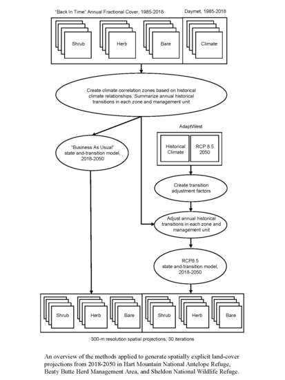
1. Introduction
A common approach for constructing a record of contemporary landscape change over large geographic areas is land-cover change analysis using multi-decadal observations made with Earth Observation Systems. Long-term monitoring provides foundational information on the rates and patterns of change, and these data can directly feed into research focused on the cause and effects of change [1]. The growing availability of free imagery and computational advances such as cloud computing have ushered in a new era of land-cover change monitoring characterized by monthly-to-annual timesteps and maps generated at regional-to-national scales [2]. A new generation of mapping efforts capitalizes on these advances, producing fractional rangeland vegetation cover at a 30-m scale, with annual time-steps, across vast landscapes [3,4]. For example, the NLCD Back in Time (BIT) project uses 30m Landsat data to generate annual fractional cover maps for different land cover types from 1985-2018 [4]. Temporally and spatially rich outputs like BIT provide a long list of benefits, such as the identification of abrupt change events across a map time series, the tracking of gradual changes over time (i.e., succession, recovery, etc.), the ability to link short-term change with drivers where comparable data exist (i.e., climate), and the opportunity to create empirical land-cover projections based on more precise estimates of change [5,6]. Chronicling historical changes and deconstructing causes of land change are also important steps towards identifying current impacts and mitigating future impacts [7,8].
An investigation into the usefulness of dense land-cover map series lies at the intersection of an inquiry where a need exists, data are available, land-use stressors are well-defined, and conservation actions can be piloted. The shrubland ecosystems that make up much of the western United States meet these criteria [9,10]. Much of these lands are federally managed, with the goal of balancing habitat conservation with regulated land use. The management of shrubland ecosystems in federal lands into the future will require an accurate understanding of past land cover change, along with the ability to understand and predict future change based on different sets of assumptions regarding the climate [11], fire dynamics, the spread of invasive species, etc. Federal land managers must also understand the impact of allowable use (i.e., grazing policy) and budgets in the development of long-term management plans. The impacts of abrupt disturbances such as fire, industrial development, and vegetation treatments on rangeland condition have been relatively well documented [4,12]. However, spatially explicit data of projected climate impacts is often lacking, constraining the prioritization of areas for climate adaptation practices [13].
In most locations the primary driver of change to vegetation composition and state are gradual agents such as longer-term climatic trends or vegetation succession [14,15] or the impacts of interannual weather variations [4]. Yet exploration of gradual change drivers (i.e., climate, vegetation succession, some land management practices) on the future distributions (i.e., patterns and abundance) of rangeland vegetation have received less attention. While deserts and semi-arid regions are among the least vulnerable to biome shift (Gonzalez et al. 2010), they are vulnerable to within-state change and droughts related to climate change since they are strongly dependent on soil water availability [16]. Recent work in the Great Basin has applied BIT map data to quantify the rates and causes of abrupt and gradual vegetation change over multiple decades [3,4,15]. Still and Richardson [17] used climate envelope modeling to project the future climate niche of Wyoming big sagebrush. Creutzberg et al. [18] used a state-and-transition model incorporating climate data through dynamic global vegetation models to investigate the potential impacts of climate change on rangeland condition in central Oregon. Homer et al. [19] projected the abundance of rangeland cover through 2050 based on several IPCC scenarios that cover a broad range of possible future climate outcomes.
According to Homer et al. [19], studying fractional vegetation change using long-term observations alongside records of precipitation change provides an opportunity to apply empirical patterns observed in the past into the future. The empirical foundation of such models makes it possible to evaluate business-as-usual scenarios projecting historical trends forward. By adjusting vegetation change probabilities in these empirical models based on the assumption that climate may change, alternative climate scenarios may be created to forecast divergent outcomes. One such way to forecast land cover change under different climate futures is to use the IPCC 5th Assessment Report [20]. This report conveys the range of possible future outcomes as Representative Concentration Pathways (RCP), which are four greenhouse gas concentration trajectories marked by radiative forcings of 2.6, 4.5, 6.0, and 8.5 Watts/meter2 [21]. These RCP emission scenarios represent, and generally correspond to, increasing rates of climate change. Specifically, the RCP 8.5 pathway represents a future with highest emissions stemming from little effort to reduce emissions and represents a failure to curb warming. Climate scenarios based on RCP 8.5 largely represent a future with the highest amount of climate change by the year 2100 [22].
We hypothesize that annual BIT data can be applied to summarize and project climate related changes in federally managed lands in the northern Great Basin. To better understand how climatic factors contribute to sagebrush (Artemisia tridentata spp.) dominant ecosystems, we conducted a historical land cover change assessment and created future land cover projections across three US Department of Interior (DOI) managed units; US Fish and Wildlife Service (USFWS) Hart Mountain National Antelope Refuge (NAR), Bureau of Land Management (BLM) Beaty Butte Herd Management Area (HMA), and USFWS Sheldon National Wildlife Refuge (NWR). We chose these areas in anticipation that results will help federal managers develop targeted management plans based on locations where vegetation cover may be changing as a result of climate. We summarize all historic fractional cover changes for shrub, herbaceous, and bare ground from the annual BIT data by comparing the fractional cover transitions from one year to the next in the sequence from 1985–2018. We focus solely on climate related changes and remove known fire and treatments from the analysis. These changes serve as the empirical foundation of a business as usual (BAU) scenario which we use to model the effect of historical trends into the future. Since anthropogenic climate change was already ongoing in the 1985–2018 time-frame [13,23], our BAU scenario is commensurate with the degree of climate change and variability (and vegetation relationships to that change) observed in this time period. Note that our BAU scenario is not based on assumptions regarding the continuation of current energy/economic policy, rather the empirical data observed in the historical period. Empirical change rates are modified based on RCP 8.5 climate projections to create a climate-change scenario. Project design assumed that the BAU scenario would represent a baseline case comparable to RCP 4.5 or RCP 6.0. The selection of RCP 8.5 as our second scenario was intended to capture the climate change that corresponds to a high emission scenario. Past research suggests that RCP 8.5 captures the upper limit of vegetation change. For example, Ford et al. (2018) found that rangeland vegetation tended to be more variable on an interannual basis for RCP 8.5 than for RCP 4.5 [24]. Further, Sanford et al. (2014) suggested that lower emission scenarios were unlikely based on current trajectories [25]. For these reasons, we opted to focus on our historical (BAU) scenario and a RCP8.5 adjusted scenario. To help generate 20–30-year climate management plans, spatially explicit BAU and RCP 8.5 projections are developed to explore mid-term land-cover effects 32 years into the future (2018–2050).
2. Methods
2.1. Study Area
Starting in the early 1930s, large tracts of land were set aside along the Oregon-Nevada border to be federally managed, with wildlife conservation, livestock production, and recreation as the intended uses. Hart Mountain NAR, Beaty Butte HMA, and Sheldon NWR are three of the management areas located in this part of the Great Basin. All three preserves are generally characterized as shrubland ecosystems primarily occupied by sagebrush species, much like the larger Great Basin. The dominant sagebrush steppe vegetation community is typified by low-to-moderate sagebrush density with a moderate presence of perennial grasses (Figure 1), but the composition of this vegetation varies between management units. At lower elevations and in more saline soils shadcale (Atriplex confertifolia) and greasewood (Sarcobatus spp.) occur. At higher elevations, stands of bitter brush (Purshia tridentata) and mountain mahogany (Cercocarpus ledifolius) become more abundant and the perennial forb community more strongly expressed. Sagebrush rangelands provide habitat for many sagebrush-obligate species, most notably the Greater sage-grouse [26].
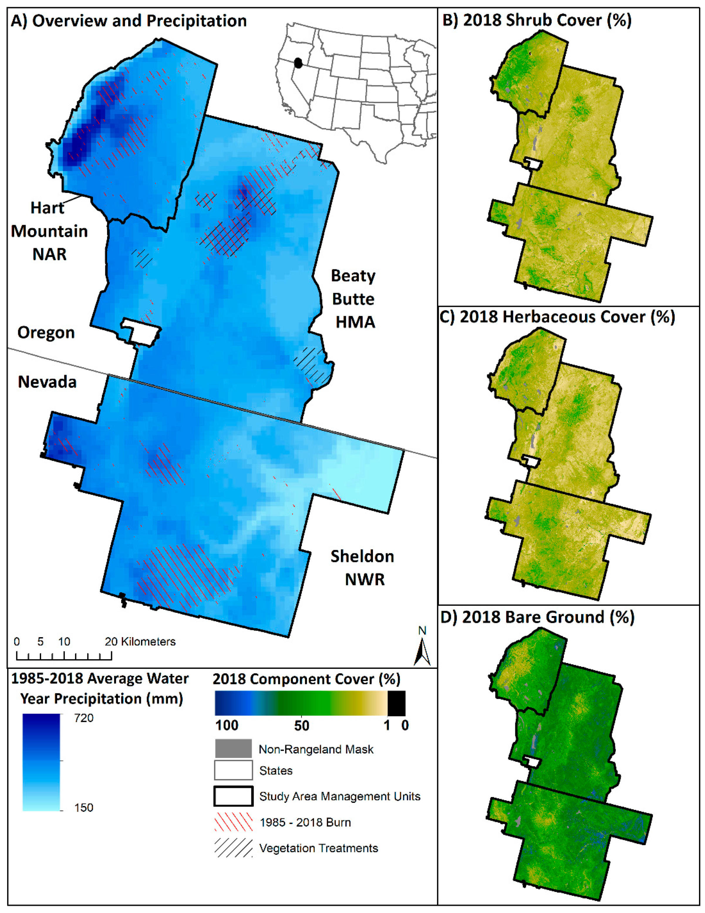
Based on 1985–2018 Daymet climate data [27] water year (October to September), climate average precipitation is 360 mm across the study area, with a minimum of 150 mm occurring in Sheldon NWR and maximum of 720 mm occurring in Hart Mountain NAR. Water year average daily maximum temperature across the study area is 13.0 °C and average daily minimum is 0.0 °C. Elevation in the study area ranges from 1293–2412 m. Climate patterns are strongly related to elevation; precipitation and temperature are positively and negatively associated, respectively. The vegetation in these ecosystems are constantly undergoing fine scale changes, but these changes are quite heterogeneous over space [4,28]. While directly adjacent to one another, each management area has a unique land-use history based on different biogeographic characteristics and contrasting management practices. From 1985–2018, 13.8% of Hart Mountain NAR, 12.0% of Sheldon, and 8.7% of Beaty Butte were burned, according to Burned Area Essential Climate Variable (BAECV) and Monitoring Trends in Burn Severity (MTBS) fire data [29,30]. Grazing by livestock ceased in 1992 in Sheldon NWR Refuge and in 1994 in Hart Mountain NAR, where removal of feral horses started in 2003 [31]. Beatty Butte HMA has been continuously grazed by livestock over the study period.
2.2. Data and Methodology
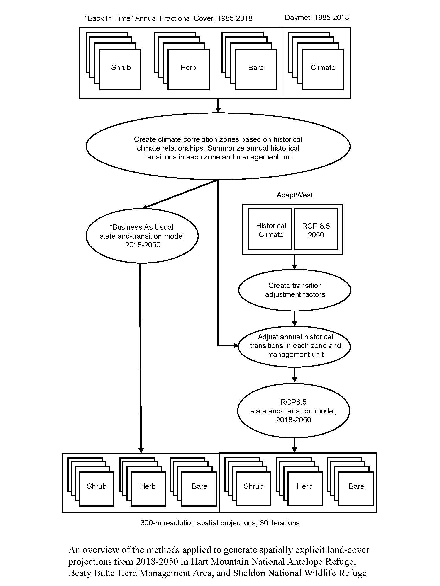
We evaluate the relationship between annual NLCD BIT fractional cover maps and Daymet temperature and precipitation data in the historical reference period. We directly use contemporary rates of change and causal relationships to create an empirical Business as Usual (BAU) land cover scenario. Historical transitions were adjusted to create a second Representative Concentration Pathways (RCP) 8.5 land cover scenario based on the difference between reference and projected RCP 8.5 climate data [32,33] (Figure 2).
2.2.1. Input Data
The primary data input to our study is the NLCD BIT fractional cover maps produced annually for 1985 to 2018 across the western U.S. [3,4]. Each 30-m pixel for a given annual BIT product shows the percent of the pixel covered (i.e., fractional cover) by the mapped cover type. The BIT suite consists of the fractional cover of shrub, sagebrush, herbaceous, annual herbaceous, litter, and bare ground. The shrub layers include sagebrush and other shrub types, while the herbaceous layers include exotic grasses and other herbaceous cover types.
The BIT products were trained from circa 2015 fractional cover base maps. The base map was trained with cover measurements collected on high-resolution (2-m) satellite images (n = 331) including World View 2, Quickbird, and Pleiades [34]. Cubist regression trees (RuleQuest Research 2008) were used to predict fractional cover over high-resolution image extents. Cover predictions were degraded to 30-m to serve as training for regional predictions using Cubist regression trees which included three seasons (spring, summer [peak-greenness], and fall [leaf-off]) of Landsat imagery, topographic variables, and spectral indices as inputs.
Next, the BIT process compared spectral change, band-by-band, between summer and fall images from all years to baseline summer and fall images from a 2014 base. A change fraction approach was used to evaluate the magnitude of change in a given pixel in each year relative to the base year, assigning a 0–100% confidence of change for each pixel. Pixels were flagged as changed if thresholds were exceeded in both summer and fall images in a given year. Training data from the circa 2014 base were selected within the unchanged pixels in each year [28,34,35]. The training points were pooled across time to develop Cubist regression tree (RuleQuest Research 2008) models which used two seasons (summer and fall) of Landsat imagery, topographic data, and spectral indices as inputs [28,34]. The Cubist models predicted fractional cover in each year across an entire Landsat path row, but the predictions were only applied in the pixels and times detected as changed, with the base map fractional cover values maintained in unchanged areas. A series of post-processing models were applied to ensure accurate post-burn trajectories and to eliminate noise and illogical change. For more details on the process, see Rigge et al. [35].
In the current study, we elected to analyze the shrub, herbaceous, and bare ground fractional cover layers as these cover types encapsulate most of the variability in structure over space and time. We used the portion of the annual BIT data generated for Landsat path 43, row 31 that intersects the three managed areas included in this study. Our study area consists of the 80% of the three management areas within the path row; large portions of Hart Mountain NAR and Beaty Butte HMA along with all of Sheldon NWR fall within the processed Landsat scene (Figure 1).
2.2.2. Data Preparation
The 30-m shrub, herbaceous, and bare stacks were clipped to the study area extent and converted to thematic layers. Difference maps were created by comparing one year to the next to measure fractional cover transitions occurring across the time series for each pixel. All pixel transitions from one fractional cover to another were summarized (i.e., 11% shrub to 13% shrub, 13% shrub to 11% shrub, etc.). Water, treatments largely intended to remove exotic annual grasses and speed post-fire recovery, and fire information (MTBS, BAECV) were used to mask out unique from-to transitions that were unlikely to result from climatic changes. The following sections describe how these transitions were incorporated into the state-and-transition modeling software.
For the time period corresponding with our BIT data, we used Daymet climate data [27]. We resampled the original 1-km data to 30m to match the BIT spatial resolution. We generated three annual climate variables using Daymet: (1) water year (October-September) average minimum temperature (TMIN), (2) water year average maximum temperature (TMAX), and (3) water year total precipitation (PRCP), for each year 1985–2018. For each cover type, we performed a Pearson correlation (r) between BIT percent cover and Daymet precipitation and temperature data at each pixel for 1985–2018. We found that the correlation coefficients were very similar between TMIN and TMAX, but TMIN tended to be more strongly correlated as observed by Shi et al. (2018), so we decided to only assess TMIN and PRCP. Correlation coefficients for each cover type were classified on three-by-three matrices (Table 1) of significant (p < 0.10) negative correlation, non-significant correlation, and significant positive correlation with PRCP and TMIN. The nine possible positions on the matrices were used to group into spatial zones of climate significance, which, along with the management units, were used to stratify historical transitions for each cover type (see ‘tertiary stratum’ in Section 2.2.3). These zones were also used in the RCP 8.5 adjustment process described in the same Section.
2.2.3. Business as Usual (BAU) and Representative Concentration Pathway (RCP) 8.5 Scenarios
For each transition from one fractional cover class (equivalent to pixel cover percentage) to another, we summarized the annual transition history to supply the model with a historical distribution to sample from. These transitions, summarized for each nested managed unit (secondary stratum) and climate zone (tertiary stratum), were applied as “transition targets” to a 2018 land cover map representing “states”. Together, the model applies ‘transitions’ to each ‘state’, randomly selecting from the historical distribution to model change spatially across the study area. Transitions are applied annually in 30 Monte Carlo model simulations.
These empirical parameters make up the Business as Usual (BAU) scenario intended to model the effect of historical trends into the future. The BAU scenario presumes that climatic and land cover variability in the 32 years after 2018 will fall within the same range as the prior 33 years. For the projection period (2018–2050), each model randomly sampled from the historical distribution of change to account for years where dry/wet or cool/warm conditions may have led to different rates of change. Applying these rates randomly over multiple simulations generates as range of possible land cover outcomes based on the underlying climate in the years that the software randomly selects. For example, a situation where the model randomly selects from the upper end of the historic distribution for a transition like shrub 40% to shrub 30% may lead to a simulation representing a future characterized by a large decline in shrub cover.
A RCP 8.5 climate change scenario was created by modifying empirical transition rates to create new fractional transition probabilities based on underlying RCP 8.5 climate projections summarized by AdaptWest [32,33], a non-governmental organization spatial database promoting adaptation to climate change in North America. An ensemble of 15 Coupled Model Intercomparison Project phase 5 (CMIP5) 2050 projections available from AdaptWest was used to estimate the average climate change across a suite of RCP 8.5 models. Monthly variables were used to generate a summary of total precipitation and minimum temperature in RCP 8.5 projections and historical data from 1981–2010 [32], and the differences were summarized for each correlation zone. The relative differences between the historical and projected period were used to adjust historical transition rates to represent climate-adjusted land cover change rates.
To accomplish this, we calculated the average historical and future (2050) PRCP and TMIN for each climate correlation zone. Next, we calculated the ratio of historical to future values of both climate variables. For example, given a historical average PRCP value of 233 mm and future value of 241 mm, the ratio would be 1.03 (241/233 = 1.03). We normalized the ratio values for PRCP so the mean across strata was similar to that of TMIN, thereby giving both variables equal weight. Finally, we took the average of PRCP and TMIN ratio by strata, giving the total climate forcing effect for each cover type separately. It is important to note that this workflow assumes that the directional relationships observed in the historical period will persist in the future; for example, areas with a positive relationship between precipitation and herbaceous cover are expected to continue this association in the future.
2.2.4. State and Transition Model Framework
We used the ApexRMS ST-SIM software package [36,37] to project land-cover change over a 32-year period (2018–2050) across 30 Monte Carlo simulations. The ST-SIM model is a type of non-stationary Markov Chain model. State-and-transition modeling software requires that all states and transitions are defined for all strata used in the analysis. In this study, three nested strata were used. The study area boundary was selected as the primary spatial stratification unit, the three DOI units were applied as the secondary stratum, and the climate correlation zones generated for each cover type (Table 1) were used as the tertiary stratum. This design allows unique transitions, relationships, and management plans to be tested. The study area was subdivided into 300-m-by-300-m simulation cells resulting in a total area of 5350 km2, with each cell assigned as study area (primary stratum), DOI unit (secondary stratum), and climate correlation zone (tertiary stratum).
For each model, the initial conditions were defined by assigning states to simulation cells based on fractional cover at the end of the observed period (i.e., 2018). As noted earlier, transitions between fractional cover classes were developed using empirical year-to-year transitions compiled from a 33-year time-series of historical map data. Most shrub pixels typically changed ±5% over the course of a single year during the historical period, while herbaceous pixels typically changed ±10%, and bare pixels typically changed ±15%. All fractional transitions that changed by more than 1% between years and exceeded 1 ha (0.01 km2) in any year across the time series were summarized for each climate zone (tertiary) in each management unit (secondary) and applied as transitions in model runs. The final two rules were applied to constrain the model to meaningful transitions while also reducing computational demand.
In summary, BAU and RCP 8.5 scenarios were generated for shrub, herbaceous, and bare ground spanning 2018–2050. Each scenario was run 30 times (also known as Monte Carlo simulation) to represent the variability between transition targets. Non-spatial state and transitions were produced annually, and 300 m spatial state class maps were produced every 5 years. The same rules were applied over the historical period to determine if the model generated outputs consistent with observed changes. Empirical changes for shrub, herbaceous, and bare ground from 1985–2018 were used as observed targets within the model, and 300 m model outputs were generated for 2018 (using 1985 maps as initial starting conditions). The comparison between the 2018 observed maps and 2018 modeled maps indicates that the model operates as expected (see Figure S1).
To ensure logical consistency across all model simulations, simulations of bare ground were manually regenerated by adding pixels values for coincident shrub and herbaceous models with fixed litter estimates from the 2018 NLCD BIT litter layer. A bare ground value was assigned for each pixel based on achieving a total fractional cover of 100 (100 − (shrub + herbaceous + litter) = bare ground). The results consist of an assessment of spatial map projections for both scenarios across the study area and within each management unit. Fractional cover is periodically aggregated into four general categories (1–20%, 21–40%, 41–60%, and 61–100%) to simplify reporting, but is expressed in finer detail in the Supplementary Materials (Tables S1–S3) and in the spatial files available on USGS ScienceBase [38].
3. Results
3.1. Historical Land Cover and Climate
Over the historical period (1985–2018), BIT map layers indicate shrub cover increased, herbaceous cover decreased, and bare ground increased in the unburned and untreated parts of all management areas (Figure 1). Over the same period, precipitation slightly decreased, and minimum temperature strongly increased. Overall, fractional cover is more strongly correlated with both TMIN and PRCP in wetter sites as compared to drier sites.
Interannual variation in fractional cover was tightly linked with PRCP and TMIN fluctuations (Table 2). Bare ground was negatively correlated with PRCP in most (66%) pixels. However, 62% of shrub and 68% of herbaceous cover pixels were positively correlated with PRCP. Bare ground, shrub, and herbaceous cover was positively correlated with TMIN in 39, 48, and 54% of pixels, respectively. Sensitivity to climate varies within the range of cover values for each cover type. For example, pixels characterized by higher bare ground cover exhibit less climate sensitivity than those with higher vegetation cover.
The strength and direction of these climate relationships laid the groundwork as weighting factors for our RCP scenarios. As previously described, we intersected the historical climate relationships (positive correlation, negative correlation and no correlation) for PRCP and TMIN to produce a three-by-three matrix and then determined the mean historical and future climate variables for each of nine zones. The assumptions of this approach are that (1) historical relationships with climate are driven in part by biophysical conditions that will persist into the future, (2) management practices will continue as implemented in 2018 into the future, and (3) vegetation compositional changes will mostly consist of in-state change that will not disrupt preceding climate relationships.
3.2. Overall Trends from 2018 to 2050
As of 2018, most (75%) of the Landsat pixels that make up the study area were classified as having less than 20% shrub cover (Figure 3). In both the BAU and RCP 8.5 scenarios, the model projects that the shrub cover in these pixels will increase. This pattern is observed in most of the 30 simulations, and on average, is only slightly more pronounced in the RCP 8.5 scenario relative to the BAU scenario (Figure 2). In most cases, the amount of shrub cover at the pixel scale is increasing towards moderate shrub cover (21–40% fractional cover) (Table 3A,B). While approximately 3600 km2 of the study area may transition but remain within the same generalized class between the start and end of the model period, the RCP 8.5 and BAU scenarios suggest that an average of 889 km2 and 1255 km2 converts to higher shrub cover classes from 2018–2050, respectively.
On average, herbaceous and shrub cover make up a similar percentage of each pixel in the study area. As of 2018, 66% of the study area was represented by less than 20% herbaceous cover while just over 33% had 21–40% cover (Figure 4). Over the projection period, this group of moderate herbaceous pixels declined in most RCP 8.5 and BAU simulations. On average, the 21–40% category declined by 310 km2 and 296 km2 in the RCP 8.5 and BAU scenarios respectively, although some individual simulations projected substantially greater losses in this category. The group with low fractional cover (1–20%) was highly variable between simulations in both scenarios, capturing some of the losses from the 21–40% group (Table 3C,D). The magnitude and variability of all transitions were more pronounced in the RCP 8.5 scenario compared to the BAU scenario (Figure 4, Table 3C,D).
Bare ground represents a sizable fraction of most pixels in the study area. It is not uncommon for a pixel to be made up of about 20% shrub cover, about 20% herbaceous cover, and more than 50% bare ground. In 2018, 58% of the study area pixels were represented by 41–60% bare cover (Figure 5). Nearly 19% of the study area has bare ground in the 21–40% category, and another 19% is in the 61–100% category. The RCP 8.5 and BAU scenarios indicate that an average of 291 km2 and 270 km2 converts from 41–60% bare ground over the 32-year study period. The RCP 8.5 scenario models more transitions to lower percent cover as compared to the BAU scenario, with 1392 km2 and 1355 km2 in conversions to lower categories, respectively (Table 3E,F). Conversely, the BAU scenario models more transitions to higher percent cover categories (1332 km2 compared to 1319 km2). Both scenarios include roughly 2700 km2 that underwent bare transitions between the start and end of the model period but remained within the same general category. In summary, the RCP 8.5 scenario produces similar patterns as the BAU scenario with slightly more pronounced shifts from moderate to low bare ground.
3.3. Management Unit Trends from 2018 to 2050
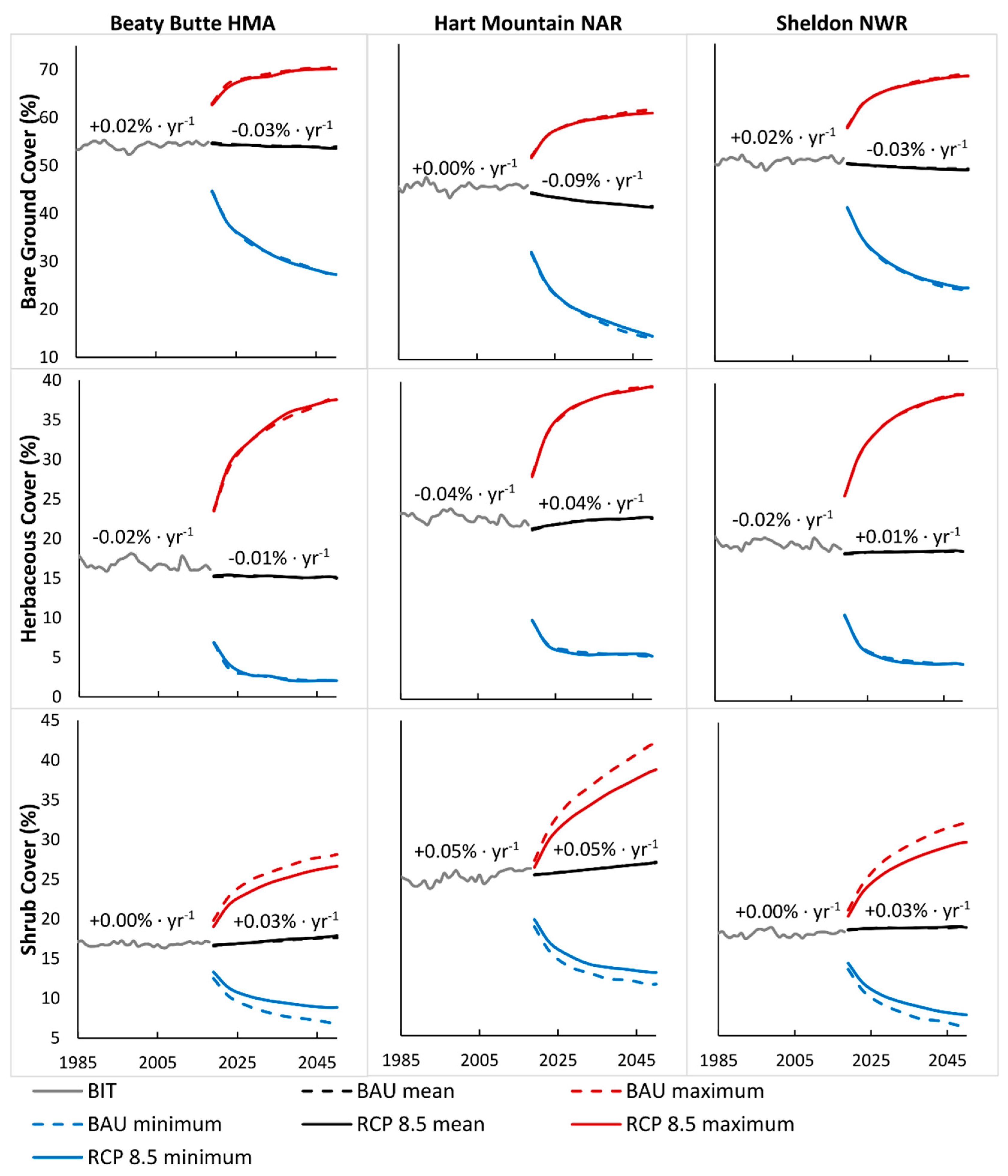
Shifting from overall cover class abundance (Figure 3, Figure 4 and Figure 5) to an assessment of average fractional cover computed for each management unit helps illustrate the overall impact of fluctuations on class composition (Figure 6). The subtle decline in average bare ground in each unit is countered by a flat to subtle increase in average herbaceous cover, and a projected increase in average shrub cover. The average fractional covers differ by <1% for bare and herbaceous cover between the BAU and RCP 8.5 scenarios when summarized at the management scale, but average shrub cover is projected to differ by 2–5% between scenarios.
While net changes for each cover type may be small after averaging across management units, slopes varied substantially spatially (Figure 7, Table 4). Spatial patterns of fractional cover slope projections reveal coherent patterns. Net landscape change between 2018 and 2050 show a projected total decrease of −0.88% and −0.99% bare ground and −0.44% and −0.45% herbaceous cover for the BAU and RCP scenarios, respectively. These decreases in bare ground and herbaceous cover are offset by a net increase of 0.71% and 0.85% in shrub cover in the BAU and RCP scenarios. The trend in all three cover types was strongest in Hart Mountain NAR and weakest in Sheldon NWR for both scenarios.
The change trend over the projected period is reported as a slope to represent the rate of change. An analysis of cover projections against other spatial variables suggests that projected cover temporal slope varied by elevation, the baseline cover in 2018, and the slope of other cover types (Table 4). Bare ground slope was positively associated with elevation, 2018 herbaceous cover, and 2018 shrub cover, and negatively associated with 2018 bare ground. Conversely, herbaceous and shrub cover slopes were negatively associated with elevation, 2018 herbaceous, and 2018 shrub cover, and positively associated with 2018 bare ground. Considered across cover types, these patterns show symmetry in the projections: locations with increasing bare ground have decreasing herbaceous and shrub cover, and vice versa. The redistribution of cover relative to the cover composition in 2018 is also an interesting indicator of how different the distribution of each cover type may be in the future. For all cover types, the slope is negatively correlated to its cover in 2018. Locations with low bare ground cover in 2018, for example, had the greatest increase in bare ground by 2050, with the opposite being the case for pixels with high bare ground cover in 2018.
4. Discussion
The management of shrubland ecosystems in the future will require the ability to understand the rates and causes of past changes to better predict future changes. While chronicling historical land cover changes and deconstructing causes of land change are important steps towards identifying current impacts and mitigating against future impacts, developing reliable models to represent the wide range of possible outcomes can be a lofty goal, especially when land use practices, management actions, invasive species distributions, fire regimes, and underlying climate may change over space and time.
In some ways, federally managed lands in the northern Great Basin are ideal testing grounds to explore how historical causes of land cover change may alter land cover into the future because annual land cover data are readily available and land-use stressors are well-defined. For example, the cessation of cattle grazing in UFSWS lands in the early 1990s is well documented, and we were able to use ancillary data to remove fire and treatments before quantifying the effects of climate. On the other hand, large interannual weather variations, the inability to disentangle spatiotemporal horse grazing impacts, and continued cattle grazing in Beaty Butte HMA makes this area difficult to study. Our investigation was built with a reasonable goal of focusing on a subset of the issues that may contribute to land cover change in federal lands in the future to inform 20–30-year climate management plans. By masking out fire and land treatments, we were able to summarize historical rates of change using annual BIT data from 1985–2018, establish how climate contributed to these changes, and project climate related changes into the future for Hart Mountain NAR, Beaty Butte HMA, and Sheldon NWR. Historical changes served as the empirical foundation of a business as usual scenario intended to model the effect of historical trends into the future, and these rates were modified based on RCP 8.5 climate projections to create a climate-change scenario intended to show how climate change may lead to different land cover distributions under the direst scenario projected by IPCC.
4.1. Historical Change
The historical assessment of land cover sensitivity to climate within the study area allowed us to detect and quantify historical land cover-climate interactions and use these relationships to create future land cover projections and helps contribute to the understanding of how climate may influence vegetation communities in the future. Our results support prior findings in this ecosystem that climate contributes to slow composition changes often undetectable in traditional remote sensing land cover changes studies [39]. We successful tracked subtle changes in fractional cover at the pixel level and established temporal correlations to precipitation and temperature across the study period (1985–2018). Correlations between cover type and climate varied substantially over the study area, even within each cover type. However, in general, bare ground was negatively correlated to PRCP and TMIN, and shrub and herbaceous cover were positively correlated to PRCP and TMIN. The strength and direction of these climate relationships served as weighting factors for our RCP scenarios, where the relative difference between the historical climate and projected climate (using a RCP 8.5 ensemble approach) were used to adjust historical transition rates in each climate correlation zone to represent climate-adjusted land cover change rates.
4.2. Projected Change
RCP 8.5 climate projections suggest that total annual PRCP will be on average 7.6 mm higher and TMIN will be 1.2 °C warmer in the study area by 2050 relative to the 1985–2018 baseline. Climate differences between the historical and projected period were relatively small over the study area: the PRCP and TMIN in the correlation zones for each cover type typically varied by ±1% among zones (i.e., standard deviation). This means that the climate change magnitude (e.g., delta) used to adjust RCP 8.5 transition targets were also generally consistent within each cover type. In the most extreme cases, negative correlations led to a fractional cover 16–18% lower than the historical period, and positive correlations generally led to a cover 21–25% higher than the historical period. In many of the zones with mixed correlation direction effects, adjustments factors were quite low and climate-adjusted transition targets were not substantially higher than BAU targets.
Relatively modest adjustments between scenarios resulted in moderate differences in the amount of change for each cover type. BAU and RCP 8.5 scenarios project different change rates across low, moderate, and high cover classes, where the magnitude of all transitions was more pronounced in the RCP 8.5 scenario compared to the BAU scenario. This led to more variability across RCP 8.5 Monte Carlo simulations as well. In the bare ground models, the RCP 8.5 scenario produces similar patterns as the BAU scenario with slightly more pronounced shifts from moderate to low bare ground. Despite some differences in the amount of fractional cover, the scenarios do not lead to substantially different average fractional cover at the management unit scale. This suggests that the BAU and RCP 8.5 scenarios result in somewhat similar landscape composition by 2050.
One possible explanation for this finding is that the BAU scenario encapsulates 34 year of climate variability (including dry, wet, cold, and hot years), and the model randomly selects transitions within the historical range. While the average precipitation and temperature is lower over the reference period compared to RCP 8.5, individual years over the reference period may have had more total precipitation or a warmer minimum temperature, and upper limit change rates reflect extremes during these anomalous years. A small difference between the BAU and RCP 8.5 scenario will occur if an adjusted RCP 8.5 transition is randomly selected from middle of the target distribution. This would lead to more change than the same transition rate (pre-adjustment) but may not exceed the upper transition limits over the reference period. In summary, climate conditions in 2050 under RCP 8.5 are most likely not novel to the range of conditions experienced in the reference period unless adjusted transition rates from the upper limit of the target distribution are consistently sampled by the modeling software.
A second explanation for the lack of major differences between BAU and RCP 8.5 results may be linked with the climate change trends already manifested in the historical period, which to date have been approximately tracking that of RCP 8.5 [23]. Indeed, past climate change is risk factor for future vulnerability, since there is often a time lag between shifts in climate and community structure [13]. Moreover, Tietjen et al. [16] found qualitatively similar results in climate vulnerability between RCP 4.5 and 8.5.
Nevertheless, the aggregated effect of hundreds-to-thousands of possible transitions modeled annually leads to some major changes in the study area between 2018 and 2050. Across the entire study area, those pixels with high bare ground in 2018 are projected to become less bare ground dominant; pixels with current moderate herbaceous cover are projected to contain less herbaceous cover, and pixels with current low shrub cover are projected to contain more shrub cover by 2050.
While overall results suggest that the entire landscape will undergo some level of change by 2050, we identified locations with higher sensitivities to projected change. Places like Hart Mountain NAR represent hotspots in the study area marked by higher climate sensitivity and are projected to have more changes by 2050. Hart Mountain NAR is projected to see the greatest decline in bare ground cover (0.09% decline in cover per year averaged across all pixels), the greatest increase in herbaceous cover (0.04% increase in cover per year), and the greatest increase in shrub cover (0.05% increase in cover per year). It has a higher elevation and a cooler, wetter climate than other parts of the study area, and these characteristics may help it have higher ecosystem resilience. Beaty Butte HMA regularly has more total transition land area, which is in part due to the size of the management unit. However, the change trends during the modeled period in Beaty Butte are much flatter than Hart Mountain, with 0.03% per year decline in average bare ground, 0.01% per year decline in herbaceous cover, and 0.03% increase in shrub cover. However, as with the overall trends, composition trends in Beaty Butte HMA are similar by cover type and management in both scenarios. Even where upper and lower limits across Monte Carlo simulations may suggest that the scenarios deviate in the shrub projections, averaging change across simulations leads to a similar outcome between scenarios in every management unit.
Specific locations are more susceptible to inter-annual climate variation, and to long term climate trends. In the historical period, we observed climate sensitivity was higher in sites with low bare ground cover, high vegetation cover, relatively high long-term mean precipitation, cooler maximum and minimum temperature, higher interannual variation in climate variables, and in burned areas. Overall, this infers more mesic sites are more sensitive to climate in our study area. These patterns carried into future projections where the greatest increases in bare ground by 2050 occurred in pixels with low bare ground cover in 2018.
4.3. Results in the Context of Past Research
Our projections of increasing shrub and decreasing bare ground in our study area seem at odds with the projections of increased TMIN and slightly increased PRCP by 2050. These climate conditions would generally be expected to produce a somewhat more xeric environment. While the direct effect of climate change is often increased precipitation across much of North America, the commensurate increase in biomass could result in a higher risk of ecological drought [16]. However, our study area is generally within a region identified as low risk for becoming unsuitable in climate for sagebrush by 2100 [40] and within the climatic and ecohydrological potentially suitable habitat in 2100 modelled by Schlaepfer et al. [41]. Moreover, relative to the 1985-2018 climate across the western U.S. range of sagebrush, our study area mean values are at the 68th percentile of PRCP and 28th percentile of TMIN. This climate results in relatively cool and moist sagebrush steppe, which in central Oregon [42] and southeast Oregon [18] was found to be relatively resilient in climate simulation and increased by mid-century, suggesting that our study may be somewhat TMIN limited. Similar increases to sagebrush cover by 2100 were projected in the northern and high-altitude portions of the western U.S. [41]. Warm–dry sagebrush types, however, were modelled to increase by mid-century but decrease by the end [18]. Salt desert scrub and xeric shrub steppe was the primary occupant of vacated sagebrush habitats by the last decades of the 21st century unless exotic annual grasses fill these locations in preceding decade. Projections suggest that grasslands will continue to represent a minor part of the landscape compared to sagebrush. Indeed, there is evidence of increasing woody vegetation in temperate drylands globally, and projections for this trend to continue [16]. Under the no climate change scenarios, sagebrush steppe and potentially suitable greater sage-grouse (Centrocercus urophasianus) habitat fared worse, with reduced extent, than under climate change scenarios [18,42].
Our study is subject to several limitations and assumptions; we do not consider the potentially great impacts of fire, grazing, and land management to land cover in our study area. While we do not explicitly consider the influence of historical or future fire, Creutzberg et al. [42] found a dramatic increase (up to 6x baseline) in fire occurrence, resulting in increased exotic grass, whose spread was ineffectively addressed by restoration. The herbaceous models do represent all types of grasses, including annual exotic grasses, but neglect to adjust changes rates based on factors beyond climate change. We also did not consider climate-grazing interactions. Livestock production is the most widespread commercial use of public lands [43], especially in Beaty Butte HMA. Horses and native ungulates are also expected to impact vegetation distributions and trends [42,43], but we neither considered how grazing may contribute to change nor how management practices, such as the removal or curtailment of livestock, may dampen the rate of change.
4.4. Future Directions
While we excluded fire, land use, and management from our models, constructing constrained land cover models in a state and transition framework has been proven to be an effective rangeland management decision support tool for considering individual influences [44]. Our modification of such models to focusing on how climate contributes to vegetation change provides an added level of refinement by isolating a specific driver. Nevertheless, the assumption that 2050 RCP 8.5 ensemble projections represent the largest deviations from historical climate and comparing RCP 8.5 projections with BAU projection may convey alternative future outcomes may be a fallacy. The Daymet climate analysis suggests that the study area had large interannual variations in total precipitation over the reference period: 50 percent year-over-year changes in precipitation were not uncommon within the study area [22]. The consistency between scenarios may be an indication that historical and projected climate may not be divergent enough to lead to truly alternate land cover outcomes. It is entirely possible that that we have already evaluated a large enough range of climate variance over the refence period that the projected RCP 8.5 climate is within that variance. Another explanation may be that the relatively small differences in climate represented by 2050 RCP 8.5 ensemble projections only led to modest adjustment factors and the resulting difference in converted area totals did not contribute to large net differences relative to the BAU scenario. We had hypothesized that compounding these small changes over time would have a larger effect, but results suggest otherwise. Similarities in the types and pattern of projected change may also be a result of the model parameterization process. Transitions were constrained to correlation zones nested within managements units, which may explain why change patterns (i.e., hotspots of change) were generally consistent between scenarios. It is also possible that amplifying the rate of change for each cover type in zones with positive precipitation and temperature correlations while reducing the rate of change for the same cover type in zones with negative precipitation and temperature correlation (i.e., spatial averaging) may have offset the net effect of the projected climate change.
The relationship between vegetation and climate relies on climate data summarized as an annual average, which follow other studies that have found mean annual precipitation to be a strong indicator of shrub and grass change across North America [45]. Nevertheless, a growing body of work in other ecosystems have considered how vegetation responds to a wider range of climatic variables [3,4,46]. A future extension of this work may benefit from testing seasonal or lag metrics, to determine if vegetation exhibits more sensitivity to different variables.
Between considering additional driving forces, more climate projections, or different climatic relationships, this proven workflow is flexible and can be adapted to adjust assumptions and incorporate more complexity. Future research should focus on including more climate models and extending the projections period while simultaneously working to resolve computing limitations. Doing so may help shed more light on long term impacts of climate, especially since RCP 8.5 is expected to have more pronounced climate change beyond 2050 and vegetation trends may experience more drastic shifts in the latter half of the 21st century, with +4.5 °C mean annual minimum temperatures and +79 mm total annual precipitation in the study area by 2100 compared to the 1981–2010 period [21,22,42]. Future model refinements may also include adding in fire simulations or different land-use constraints (i.e., grazing limits) into the model to eventually simulate drivers operating simultaneously.
5. Conclusions
Climate changes are often manifested as subtle changes in vegetation condition [46], and slow composition changes often undetectable in traditional remote sensing land cover changes studies that use multi-year intervals between observations [10,47]. Moreover, the nature of subtle change is such that it would often be missed by studies employing thematic land cover data [13,14]. While we can now use fractional cover maps to detect subtle changes in land cover composition at the pixel level, and model these changes into the future, it may be assumed that subtle changes lead to somewhat muted results. However, compounding small changes over time contributes to noticeable changes when aggregated within different DOI lands. This effort demonstrates just how much climate alone will factor into future cover change across the Great Basin in the near future. Collectively, these products will help guide land managers towards devising sustainable strategies to meet long-term goals.
Perhaps the most valuable benefit to be gained from this research is the application of state and transition modeling to visualize how climate may alter sagebrush ecosystems into the future. Quantifying the historical relationship between shrub, herbaceous, and bare cover and climate and adjusting these relationships based on future climate projections is not yet standard practice in state and transition modeling. State and transition modeling software is commonly applied to understand abrupt land-use/land-cover changes. By generating a very detailed investigation into historic and potential vegetation change based on climate sensitivity, we have successfully applied state and transition models to forecast subtle fractional cover changes into the future. Applying fractional cover changes to investigate shifts in vegetation composition at the pixel scale really tests the current computational constraints of state and transition models because so many unique transitions may occur (i.e., more than 20,000 unique transitions in the bare ground model). However, using a framework where vegetation sensitivity to climate is constrained to zones where specific relationships have been established allows any or all transitions to be easily adjusted in a tabular environment and uploaded into the modeling software based on any future climate assumption [38]. Future research should focus on generating multiple iterations of the current model based on different climate projections and extending the projections period beyond 2050 while simultaneously working to resolve computing limitations. Doing so will help shed more light on long term impacts of climate.
Supplementary Materials
The following are available online at https://www.mdpi.com/2072-4292/12/15/2360/s1. See attached figures and tables, as well as a USGS data release including the input data, model instructions, and model outputs used for this research can be found on USGS ScienceBase (https://doi.org/10.5066/P9LJ1FI4). The downloadable output maps files are organized by cover type and scenario and are available in the GeoTIF (.tif) raster file format. The 1620 TIF raster data files were created using free state-and-transition software created by ApexRMS.
Author Contributions
Conceptualization, C.E.S.; Methodology, C.E.S. and M.R.; Formal Analysis, C.E.S. and M.R.; Writing, C.E.S. and M.R.; Visualization, C.E.S. and M.R. All authors have read and agreed to the published version of the manuscript.
Funding
Funding for this work was provided by the U.S. Geological Survey Climate Research and Development Program and Northwest Climate Adaptation Science Center.
Acknowledgments
We would like to thank Jessica Walker of the US Geological Survey, Sean Finn of the US Fish and Wildlife Service, and three anonymous reviewers for their constructive reviews of the manuscript. Any use of trade, firm, or product names is for descriptive purposes only and does not imply endorsement by the U.S. Government.
Conflicts of Interest
The authors declare no conflict of interest.
References
- Fensholt, R.; Langanke, T.; Rasmussen, K.; Reenberg, A.; Prince, S.D.; Tucker, C.; Scholes, R.J.; Le, Q.B.; Bondeau, A.; Eastman, R.; et al. Greenness in semi-arid areas across the globe 1981–2007—An Earth Observing Satellite based analysis of trends and drivers. Remote Sens. Environ. 2012, 121, 144–158. [Google Scholar] [CrossRef]
- Wulder, M.A.; Masek, J.G.; Cohen, W.B.; Loveland, T.R.; Woodcock, C.E. Opening the archive: How free data has enabled the science and monitoring promise of Landsat. Remote Sens. Environ. 2012, 122, 2–10. [Google Scholar] [CrossRef]
- Shi, H.; Rigge, M.; Homer, C.G.; Xian, G.; Meyer, D.K.; Bunde, B. Historical Cover Trends in a Sagebrush Steppe Ecosystem from 1985 to 2013: Links with Climate, Disturbance, and Management. Ecosystems 2018, 21, 913–929. [Google Scholar] [CrossRef]
- Rigge, M.; Shi, H.; Homer, C.; Danielson, P.; Granneman, B. Long-term trajectories of fractional component change in the Northern Great Basin, USA. Ecosphere 2019, 10, e02762. [Google Scholar] [CrossRef]
- Sleeter, B.M.; Sohl, T.L.; Bouchard, M.A.; Reker, R.R.; Soulard, C.E.; Acevedo, W.; Griffith, G.E.; Sleeter, R.R.; Auch, R.F.; Sayler, K.L.; et al. Scenarios of land use and land cover change in the conterminous United States: Utilizing the special report on emission scenarios at ecoregional scales. Glob. Environ. Chang. 2012, 22, 896–914. [Google Scholar] [CrossRef] [Green Version]
- Lambin, E.F. Modelling and monitoring land-cover change processes in tropical regions. Prog. Phys. Geogr. 1997, 21, 375–393. [Google Scholar] [CrossRef]
- Shoyama, K.; Yamagata, Y. Predicting land-use change for biodiversity conservation and climate-change mitigation and its effect on ecosystem services in a watershed in Japan. Ecosyst. Serv. 2014, 8, 25–34. [Google Scholar] [CrossRef]
- Robinson, D.T.; Brown, D.G.; Parker, D.C.; Schreinemachers, P.; Janssen, M.A.; Huigen, M.; Wittmer, H.; Gotts, N.; Promburom, P.; Irwin, E.; et al. Comparison of empirical methods for building agent-based models in land use science. J. Land Use Sci. 2007, 2, 31–55. [Google Scholar] [CrossRef]
- Hemstrom, M.A.; Wisdom, M.J.; Hann, W.J.; Rowland, M.M.; Wales, B.C.; Gravenmier, R.A. Sagebrush-Steppe Vegetation Dynamics and Restoration Potential in the Interior Columbia Basin, USA. Conserv. Biol. 2002, 16, 1243–1255. [Google Scholar] [CrossRef]
- Soulard, C.E.; Sleeter, B.M. Late twentieth century land-cover change in the basin and range ecoregions of the United States. Reg. Environ. Chang. 2012, 12, 813–823. [Google Scholar] [CrossRef]
- Rehfeldt, G.E.; Crookston, N.L.; Sáenz-Romero, C.; Campbell, E.M. North American vegetation model for land-use planning in a changing climate: A solution to large classification problems. Ecol. Appl. 2012, 22, 119–141. [Google Scholar] [CrossRef] [PubMed]
- Barker, B.S.; Pilliod, D.S.; Rigge, M.; Homer, C.G. Pre-fire vegetation drives post-fire outcomes in sagebrush ecosystems: Evidence from field and remote sensing data. Ecosphere 2019, 10, e02929. [Google Scholar] [CrossRef]
- Gonzalez, P.; Neilson, R.P.; Lenihan, J.M.; Drapek, R.J. Global patterns in the vulnerability of ecosystems to vegetation shifts due to climate change. Glob. Ecol. Biogeogr. 2010, 19, 755–768. [Google Scholar] [CrossRef]
- Vogelmann, J.E.; Xian, G.; Homer, C.; Tolk, B. Monitoring gradual ecosystem change using Landsat time series analyses: Case studies in selected forest and rangeland ecosystems. Remote Sens. Environ. 2012, 122, 92–105. [Google Scholar] [CrossRef] [Green Version]
- Vogelmann, J.E.; Gallant, A.L.; Shi, H.; Zhu, Z. Perspectives on monitoring gradual change across the continuity of Landsat sensors using time-series data. Remote Sens. Environ. 2016, 185, 258–270. [Google Scholar] [CrossRef] [Green Version]
- Tietjen, B.; Schlaepfer, D.R.; Bradford, J.B.; Lauenroth, W.K.; Hall, S.A.; Duniway, M.C.; Hochstrasser, T.; Jia, G.; Munson, S.M.; Pyke, D.A.; et al. Climate change-induced vegetation shifts lead to more ecological droughts despite projected rainfall increases in many global temperate drylands. Glob. Chang. Biol. 2017, 23, 2743–2754. [Google Scholar] [CrossRef]
- Still, S.M.; Richardson, B.A. Projections of Contemporary and Future Climate Niche for Wyoming Big Sagebrush (Artemisia tridentata subsp. wyomingensis): A Guide for Restoration. Nat. Areas J. 2015, 35, 30–43. [Google Scholar] [CrossRef]
- Creutzburg, M.; Henderson, E.; Conklin, D. Climate Change and Land Management Impact Rangeland Condition and Sage-Grouse Habitat in Southeastern Oregon. AIMS Environ. Sci. 2015, 2, 203–236. [Google Scholar] [CrossRef]
- Homer, C.G.; Xian, G.; Aldridge, C.L.; Meyer, D.K.; Loveland, T.R.; O’Donnell, M.S. Forecasting sagebrush ecosystem components and greater sage-grouse habitat for 2050: Learning from past climate patterns and Landsat imagery to predict the future. Ecol. Indic. 2015, 55, 131–145. [Google Scholar] [CrossRef] [Green Version]
- Pachauri, R.K.; Allen, M.R.; Barros, V.R.; Broome, J.; Cramer, W.; Christ, R.; Church, J.A.; Clarke, L.; Dahe, Q.; Dasgupta, P.; et al. Climate Change 2014: Synthesis Report. Contribution of Working Groups I, II and III to the Fifth Assessment Report of the Intergovernmental Panel on Climate Change; Pachauri, R.K., Meyer, L., Eds.; IPCC: Geneva, Switzerland, 2014; p. 151. ISBN 978-92-9169-143-2. [Google Scholar]
- Wayne, G. The Beginner’s Guide to Representative Concentration Pathways. Skept. Sci. 2013, 25. Available online: https://denning.atmos.colostate.edu/ats760/Readings/RCP_Guide.pdf (accessed on 20 July 2020).
- Rogelj, J.; Meinshausen, M.; Knutti, R. Global warming under old and new scenarios using IPCC climate sensitivity range estimates. Nat. Clim. Chang. 2012, 2, 248–253. [Google Scholar] [CrossRef]
- Meyer, L.; Brinkman, S.; van Kesteren, L.; Leprince-Ringuet, N.; van Boxmeer, F. Technical Support Unit for the Synthesis Report. 169. Available online: https://www.ipcc.ch/site/assets/uploads/2018/05/SYR_AR5_FINAL_full_wcover.pdf (accessed on 20 July 2020).
- Ford, P.L.; Reeves, M.C.; Frid, L. A Tool for Projecting Rangeland Vegetation Response to Management and Climate. Rangelands 2019, 41, 49–60. [Google Scholar] [CrossRef]
- Sanford, T.; Frumhoff, P.C.; Luers, A.; Gulledge, J. The climate policy narrative for a dangerously warming world. Nat. Clim. Chang. 2014, 4, 164–166. [Google Scholar] [CrossRef]
- Rowland, M.M.; Wisdom, M.J.; Suring, L.H.; Meinke, C.W. Greater sage-grouse as an umbrella species for sagebrush-associated vertebrates. Biol. Conserv. 2006, 129, 323–335. [Google Scholar] [CrossRef]
- Thornton, P.E.; Thornton, M.M.; Vose, R.S. Daymet: Annual Tile Summary Cross-Validation Statistics for North America, Version 3. ORNL DAAC 2016. [Google Scholar] [CrossRef]
- Xian, G.; Homer, C.; Rigge, M.; Shi, H.; Meyer, D. Characterization of shrubland ecosystem components as continuous fields in the northwest United States. Remote Sens. Environ. 2015, 168, 286–300. [Google Scholar] [CrossRef] [Green Version]
- Hawbaker, T.J.; Vanderhoof, M.K.; Beal, Y.-J.; Takacs, J.D.; Schmidt, G.L.; Falgout, J.T.; Williams, B.; Fairaux, N.M.; Caldwell, M.K.; Picotte, J.J.; et al. Mapping burned areas using dense time-series of Landsat data. Remote Sens. Environ. 2017, 198, 504–522. [Google Scholar] [CrossRef]
- Eidenshink, J.; Schwind, B.; Brewer, K.; Zhu, Z.-L.; Quayle, B.; Howard, S. A Project for Monitoring Trends in Burn Severity. Fire Ecol. 2007, 3, 3–21. [Google Scholar] [CrossRef]
- Boyd, C.S.; Davies, K.W.; Collins, G.H. Impacts of Feral Horse Use on Herbaceous Riparian Vegetation Within a Sagebrush Steppe Ecosystem. Rangel. Ecol. Manag. 2017, 70, 411–417. [Google Scholar] [CrossRef]
- Hamann, A.; Wang, T.; Spittlehouse, D.L.; Murdock, T.Q. A Comprehensive, High-Resolution Database of Historical and Projected Climate Surfaces for Western North America. Bull. Am. Meteor. Soc. 2013, 94, 1307–1309. [Google Scholar] [CrossRef]
- Wang, T.; Hamann, A.; Spittlehouse, D.; Carroll, C. Locally Downscaled and Spatially Customizable Climate Data for Historical and Future Periods for North America. PLoS ONE 2016, 11, e0156720. [Google Scholar] [CrossRef]
- Rigge, M.; Homer, C.; Cleeves, L.; Meyer, D.K.; Bunde, B.; Shi, H.; Xian, G.; Schell, S.; Bobo, M. Quantifying Western U.S. Rangelands as Fractional Components with Multi-Resolution Remote Sens. and In Situ Data. Remote Sens. 2020, 12, 412. [Google Scholar] [CrossRef] [Green Version]
- Rigge, M.; Homer, C.; Shi, H.; Meyer, D.K. Validating a Landsat Time-Series of Fractional Component Cover Across Western U.S. Rangelands. Remote Sens. 2019, 11, 3009. [Google Scholar] [CrossRef] [Green Version]
- Daniel, C.J.; Frid, L. Predicting landscape vegetation dynamics using state-and-transition simulation models. In Proceedings of the First Landscape State-and-Transition Simulation Modeling Conference, Portland, OR, USA, 14–16 June 2011; Kerns, B.K., Shlisky, A.J., Daniel, C.J., Eds.; U.S. Department of Agriculture, Forest Service, Pacific Northwest Research Station: Portland, OR, USA, 2012; General Technical Report (GTR); PNW-GTR-869. [Google Scholar]
- Daniel, C.J.; Frid, L.; Sleeter, B.M.; Fortin, M.-J. State-and-transition simulation models: A framework for forecasting landscape change. Methods Ecol. Evol. 2016, 7, 1413–1423. [Google Scholar] [CrossRef] [Green Version]
- Soulard, C.E.; Rigge, M. Spatially-Explicit Land-Cover Scenarios of Federal Lands in the Northern Great Basin: 2018–2050. Data Release U. S. Geol. Surv. 2020. [Google Scholar] [CrossRef]
- Xian, G.; Homer, C.G.; Aldridge, C.L. Effects of Land Cover and Regional Climate Variations on Long-Term Spatiotemporal Changes in Sagebrush Ecosystems. Gisci. Remote Sens. 2012, 49, 378–396. [Google Scholar] [CrossRef]
- Bradley, B.A. Assessing ecosystem threats from global and regional change: Hierarchical modeling of risk to sagebrush ecosystems from climate change, land use and invasive species in Nevada, USA. Ecography 2010, 33, 198–208. [Google Scholar] [CrossRef]
- Schlaepfer, D.R.; Lauenroth, W.K.; Bradford, J.B. Effects of ecohydrological variables on current and future ranges, local suitability patterns, and model accuracy in big sagebrush. Ecography 2012, 35, 374–384. [Google Scholar] [CrossRef]
- Creutzburg, M.K.; Halofsky, J.E.; Halofsky, J.S.; Christopher, T.A. Climate Change and Land Management in the Rangelands of Central Oregon. Environ. Manag. 2015, 55, 43–55. [Google Scholar] [CrossRef]
- Beschta, R.L.; Donahue, D.L.; DellaSala, D.A.; Rhodes, J.J.; Karr, J.R.; O’Brien, M.H.; Fleischner, T.L.; Deacon Williams, C. Adapting to Climate Change on Western Public Lands: Addressing the Ecological Effects of Domestic, Wild, and Feral Ungulates. Environ. Manag. 2013, 51, 474–491. [Google Scholar] [CrossRef]
- Bashari, H.; Smith, C.; Bosch, O.J.H. Developing decision support tools for rangeland management by combining state and transition models and Bayesian belief networks. Agric. Syst. 2008, 99, 23–34. [Google Scholar] [CrossRef]
- Paruelo, J.M.; Lauenroth, W.K. Interannual variability of NDVI and its relationship to climate for North American shrublands and grasslands. J. Biogeogr. 1998, 25, 721–733. [Google Scholar] [CrossRef]
- Albano, C.M.; McClure, M.L.; Gross, S.E.; Kitlasten, W.; Soulard, C.E.; Morton, C.; Huntington, J. Spatial patterns of meadow sensitivities to interannual climate variability in the Sierra Nevada. Ecohydrology 2019, 12, e2128. [Google Scholar] [CrossRef]
- Soulard, C.E. Land-Cover Trends of the Central Basin and Range Ecoregion; Scientific Investigations Report. Data Release U. S. Geol. Surv. 2006. [Google Scholar] [CrossRef]
Figure 1.
Study area overview. (A) Management units and 1985-2018 average water year (October-September) precipitation generated from Daymet data. Also depicted are 1985-2018 burns and Bureau of Land Management vegetation treatments. Inset panel shows location of study area within the western U.S. Fractional cover of (B) shrub, (C) herbaceous, and (D) bare ground are shown for 2018.

Figure 2.
An overview of the methods applied to generate spatially explicit land-cover projections from 2018–2050 in Hart Mountain NAR, Beaty Butte HMA, and Sheldon NWR.
Figure 2.
An overview of the methods applied to generate spatially explicit land-cover projections from 2018–2050 in Hart Mountain NAR, Beaty Butte HMA, and Sheldon NWR.

Figure 3.
Business as Usual (BAU) and Representative Concentrations Pathway (RCP) 8.5 scenario results for shrub cover (km2), summarized across the entire study area. Variance and mean were calculated from across the 30 model runs. Data from 2018 have no error bars as they were observed directly using Back in Time (BIT) data. The y-axis varies between plots.

Figure 4.
BAU and RCP 8.5 scenario results for herbaceous cover (km2), summarized across the entire study area. Variance and means were calculated from across the 30 model runs. Data from 2018 have no error bars as they were observed directly using BIT data. No pixels have more than 60 percent herbaceous cover. The y-axis varies between plots.

Figure 5.
BAU and RCP 8.5 scenario results for bare ground (km2), summarized across the entire study area. Variance and means were calculated from across the 30 model runs. Data from 2018 have no error bars as they were observed directly using BIT data. The y-axis varies between plots.
Figure 5.
BAU and RCP 8.5 scenario results for bare ground (km2), summarized across the entire study area. Variance and means were calculated from across the 30 model runs. Data from 2018 have no error bars as they were observed directly using BIT data. The y-axis varies between plots.

Figure 6.
Mean fractional cover by management unit and scenario. For the Business as Usual (BAU) and RCP 8.5 projections, the minimum, mean, and maximum values across the 30 Monte Carlo simulations are provided. Linear slope rate for the BIT and projections are labeled above each mean trend line. RCP 8.5 mean overlaps the BAU mean.

Figure 7.
2018–2050 temporal slope of rangeland fractional cover for (A) Business as Usual (BAU) and (B) RCP 8.5 scenarios, based on the mean across 30 Monte Carlo simulations.
Figure 7.
2018–2050 temporal slope of rangeland fractional cover for (A) Business as Usual (BAU) and (B) RCP 8.5 scenarios, based on the mean across 30 Monte Carlo simulations.


Table 1.
Correlation zones were generated for each cover type. These zones were used as a sub-stratum in the model nested within each management unit. Historical transitions were adjusted in the Representative Concentration Pathway (RCP) 8.5 scenario for each zone based on the difference between reference and projected RCP 8.5 climate.
| PRCP Correlation | ||||
|---|---|---|---|---|
| Negative | None | Positive | ||
| TMIN Correlation | Negative | 1 | 2 | 3 |
| None | 4 | 5 | 6 | |
| Positive | 7 | 8 | 9 | |
Table 2.
Summary of component correlation relationships with climate. Values reflect the proportion (%) of 30-m cells with a given relationship to either precipitation or minimum temperature for each component. Sites with no climate relationship were defined as having correlation between each climate variable and each component with a p value > 0.90.
| Precipitation | |||
| Relationship | Herbaceous | Shrub | Bare Ground |
| Negative (p < 0.10) | 2.3 | 5.4 | 22.1 |
| Positive (p < 0.10) | 22.1 | 18.8 | 3.2 |
| Negative | 23.4 | 30.1 | 66.5 |
| Positive | 68.3 | 61.5 | 25.6 |
| None | 8.2 | 8.4 | 7.9 |
| Minimum Temperature | |||
| Relationship | Herbaceous | Shrub | Bare Ground |
| Negative (p < 0.10) | 18.2 | 11.5 | 6.8 |
| Positive (p < 0.10) | 5.9 | 9.3 | 14.3 |
| Negative | 36.5 | 41.4 | 51.2 |
| Positive | 54.2 | 48 | 39.1 |
| None | 9.3 | 10.6 | 9.7 |
Table 3.
Average transitions between categories for 2018–2050. Units are reported as square kilometers, with standard deviation across simulation marked with parentheses. The six models are labeled A–F.
Table 3.
Average transitions between categories for 2018–2050. Units are reported as square kilometers, with standard deviation across simulation marked with parentheses. The six models are labeled A–F.
| A. Shrub-BAU | 2050 Category | B. Shrub-RCP 8.5 | 2050 Category | ||||||||
| 1–20% | 21–40% | 41–60% | 61–100% | 1–20% | 21–40% | 41–60% | 61–100% | ||||
| 2018 Category | 1–20% | - | 1023(63) | 147(49) | 6(0) | 2018 Category | 1–20% | - | 708(38) | 23(30) | 40(35) |
| 21–40% | 772(13) | - | 79(18) | 2(0) | 21–40% | 521(10) | - | 82(6) | 26(7) | ||
| 41–60% | 36(1) | 30(1) | - | 0(0) | 41–60% | 2(0) | 30(1) | - | 10(1) | ||
| 61–100% | 5(0) | 2(0) | 1(0) | - | 61–100% | 0(0) | 0(0) | 0(0) | - | ||
| C. Herb-BAU | 2050 Category | D. Herb-RCP 8.5 | 2050 Category | ||||||||
| 1–20% | 21–40% | 41–60% | 61–100% | 1–20% | 21–40% | 41–60% | 61–100% | ||||
| 2018 Category | 1–20% | - | 816(30) | 90(30) | 0(0) | 2018 Category | 1–20% | - | 812(48) | 96(35) | 0(0) |
| 21–40% | 1026(18) | - | 113(24) | 0(0) | 21–40% | 1027(20) | - | 121(32) | 0(0) | ||
| 41–60% | 7(0) | 19(1) | - | 0(0) | 41–60% | 7(0) | 18(2) | - | 0(0) | ||
| 61–100% | 0(0) | 0(0) | 0(0) | - | 61–100% | 0(0) | 0(0) | 0(0) | - | ||
| E. Bare BAU | 2050 Category | F. Bare-RCP 8.5 | 2050 Category | ||||||||
| 1–20% | 21–40% | 41–60% | 61–100% | 1–20% | 21–40% | 41–60% | 61–100% | ||||
| 2018 Category | 1–20% | - | 105(4) | 39(2) | 1(0) | 2018 Category | 1–20% | - | 104(2) | 39(2) | 1(0) |
| 21–40% | 199(39) | - | 449(7) | 55(6) | 21–40% | 221(26) | - | 445(7) | 56(7) | ||
| 41–60% | 55(15) | 508(19) | - | 683(62) | 41–60% | 60(8) | 517(16) | - | 674(65) | ||
| 61–100% | 9(7) | 86(8) | 498(22) | - | 61–100% | 13(6) | 89(9) | 492(19) | - | ||
Table 4.
Correlation (r) between fractional cover slope from 2018 to 2050 by scenario and elevation, 2018 cover, and 2018 to 2050 slope of other cover types. All correlations are significant (p < 0.05).
Table 4.
Correlation (r) between fractional cover slope from 2018 to 2050 by scenario and elevation, 2018 cover, and 2018 to 2050 slope of other cover types. All correlations are significant (p < 0.05).
| 2018 Cover | 2018–2050 Slope | |||||||
|---|---|---|---|---|---|---|---|---|
| Scenario | Cover Type | Elevation | Bare | Herb. | Shrub | Bare | Herb. | Shrub |
| BAU | Bare | 0.43 | −0.69 | 0.69 | 0.45 | 1.00 | −0.83 | −0.74 |
| BAU | Herbaceous | −0.40 | 0.64 | −0.79 | −0.25 | −0.83 | 1.00 | 0.24 |
| BAU | Shrub | −0.27 | 0.42 | −0.25 | −0.48 | −0.74 | 0.24 | 1.00 |
| RCP 8.5 | Bare | 0.41 | −0.64 | 0.65 | 0.42 | 1.00 | −0.77 | −0.77 |
| RCP 8.5 | Herbaceous | −0.40 | 0.63 | −0.78 | −0.24 | −0.77 | 1.00 | 0.20 |
| RCP 8.5 | Shrub | −0.23 | 0.36 | −0.22 | −0.41 | −0.77 | 0.20 | 1.00 |
© 2020 by the authors. Licensee MDPI, Basel, Switzerland. This article is an open access article distributed under the terms and conditions of the Creative Commons Attribution (CC BY) license (http://creativecommons.org/licenses/by/4.0/).
Share and Cite
MDPI and ACS Style
Soulard, C.E.; Rigge, M. Application of Empirical Land-Cover Changes to Construct Climate Change Scenarios in Federally Managed Lands. Remote Sens. 2020, 12, 2360. https://doi.org/10.3390/rs12152360
AMA Style
Soulard CE, Rigge M. Application of Empirical Land-Cover Changes to Construct Climate Change Scenarios in Federally Managed Lands. Remote Sensing. 2020; 12(15):2360. https://doi.org/10.3390/rs12152360
Chicago/Turabian StyleSoulard, Christopher E., and Matthew Rigge. 2020. "Application of Empirical Land-Cover Changes to Construct Climate Change Scenarios in Federally Managed Lands" Remote Sensing 12, no. 15: 2360. https://doi.org/10.3390/rs12152360
Note that from the first issue of 2016, this journal uses article numbers instead of page numbers. See further details here.