Methods of Rapid Quality Assessment for National-Scale Land Surface Change Monitoring

1
ASRC Federal Data Solutions, Contractor to the U.S. Geological Survey, Earth Resources Observation and Science (EROS) Center, 47914 252nd Street, Sioux Falls, SD 57198, USA
2
U.S. Geological Survey (USGS), Earth Resources Observation and Science (EROS) Center, 47914 252nd Street, Sioux Falls, SD 57198, USA
*
Author to whom correspondence should be addressed.
Remote Sens. 2020, 12(16), 2524; https://doi.org/10.3390/rs12162524
Submission received: 26 June 2020
/
Revised: 29 July 2020
/
Accepted: 30 July 2020
/
Published: 6 August 2020
(This article belongs to the Special Issue Advancements in Remote Sensing of Land Surface Change)
Abstract
:Providing rapid access to land surface change data and information is a goal of the U.S. Geological Survey. Through the Land Change Monitoring, Assessment, and Projection (LCMAP) initiative, we have initiated a monitoring capability that involves generating a suite of 10 annual land cover and land surface change datasets across the United States at a 30-m spatial resolution. During the LCMAP automated production, on a tile-by-tile basis, erroneous data can occasionally be generated due to hardware or software failure. While crucial to assure the quality of the data, rapid evaluation of results at the pixel level during production is a substantial challenge because of the massive data volumes. Traditionally, product quality relies on the validation after production, which is inefficient to reproduce the whole product when an error occurs. This paper presents a method for automatically evaluating LCMAP results during the production phase based on 14 indices to quickly find and flag erroneous tiles in the LCMAP products. The methods involved two types of comparisons: comparing LCMAP values across the temporal record to measure internal consistency and calculating the agreement with multiple intervals of the National Land Cover Database (NLCD) data to measure the consistency with existing products. We developed indices on a tile-by-tile basis in order to quickly find and flag potential erroneous tiles by comparing with surrounding tiles using local outlier factor analysis. The analysis integrates all indices into a local outlier score (LOS) to detect erroneous tiles that are distinct from neighboring tiles. Our analysis showed that the methods were sensitive to partially erroneous tiles in the simulated data with a LOS higher than 2. The rapid quality assessment methods also successfully identified erroneous tiles during the LCMAP production, in which land surface change results were not properly saved to the products. The LOS map and indices for rapid quality assessment also point to directions for further investigations. A map of all LOS values by tile for the published LCMAP shows all LOS values are below 2. We also investigated tiles with high LOS to ensure the distinction with neighboring tiles was reasonable. An index in this study shows the overall agreement between LCMAP and NLCD on a tile basis is above 71.5% and has an average at 89.1% across the 422 tiles in the conterminous United States. The workflow is suitable for other studies with a large volume of image products.
1. Introduction
Land change science helps understand the interactions between people and nature that lead to changes in the type, intensity, condition, and location of land use and cover. It seeks to provide scientific knowledge of land use and land cover patterns and dynamics affecting the structure and function of the Earth system [1]. Knowledge about Earth’s land cover condition and how it changes over time is a critical element in a variety of environmental studies [2]. For instance, land cover change information has been widely used for assessing carbon release and sequestration [3,4,5,6], hydrologic dynamics [7,8], forest disturbance [9,10,11], urban land surface temperature [12,13], and urbanization [14].
Long-term land change information derived from remote sensing imagery can be the primary source to meet these needs. Countries and regions across the globe have produced multi-temporal land cover products, including Canada [15,16], Brazil [17,18], Australia [19], China [20,21], Europe [22,23], and Russia [24]. Moreover, advances like Google Earth Engine are increasingly enabling continental and global-scale products, e.g., [9,25,26]. The U.S. Geological Survey (USGS) has a long history of producing land cover datasets. Since the early 1970s, several major land cover datasets have been produced by the USGS Earth Resources Observation and Science (EROS) Center at both international [27] and national scales [28]. The USGS National Land Cover Database (NLCD) project has produced 30-m land cover products since 1992. The products are updated every 2–3 years for the conterminous United States. and every 10 years for Alaska [28,29,30]. However, research and applications about climate change and resource sustainability require more timely land cover and land change products [1,31]. The USGS response to this growing need is the Land Change Monitoring, Assessment, and Projection (LCMAP) initiative [32].
The USGS LCMAP has focused on implementing an innovative time-series analysis using the data-rich Landsat archive to provide land change science information and knowledge for the United States. LCMAP leverages the tile-based Landsat Analysis Ready Data (ARD) [33] and the Continuous Change Detection and Classification (CCDC) algorithm [34] to create independently validated datasets and applications to improve our understanding of natural and man-made change and address pressing questions of land and resource management. ARD contains surface reflectance data over the United States from the Thematic Mapper (Landsats 4 and 5), Enhanced Thematic Mapper Plus (ETM+) (Landsat 7), and Operational Land Imager (Landsat 8) [33]. ARD is structured in a 150 × 150 km tile scheme with the Albers Equal Area Conic projection. The CCDC algorithm builds time series models at the pixel scale to classify land cover types and detect changes [34]. LCMAP output products are structured using the same tiling system (Figure 2 in [29]).
LCMAP has been implemented for operational change detection and land cover mapping with annual temporal time steps from 1985 to 2017. Tile-based results are automatically generated from detecting day of year changes, collecting training data, and classifying time-series models. The LCMAP product suite includes five land cover and five change map products at an annual time step, including primary and secondary land cover classes and confidence layers for each, annual land cover change, time of spectral change and time since last change, change magnitude, spectral stability period, and model quality data [32]. Each product has 33 layers for 1985–2017 for the conterminous United States (CONUS) and is organized by the 150 km by 150 km tile system [33]. The final LCMAP annual product suite (doi:10.5066/P9W1TO6E) contains 422 tiles for CONUS [33], and each tile has 330 data layers (a total of 12.3GB file size for each tile). During operational production, errors could occur; for example, time series data not retrieved correctly, erroneous results due to program bugs, or results not saved properly. Thus, a quality control procedure is needed along with the production.
Traditional product quality control activities were either based on human interpretation during production [35,36] or relied mainly on validation after production was completed [37,38]. Most validation methods involve elements of sampling design, land cover identification, accuracy assessment, and land cover change validation [39,40]. LCMAP also developed a randomly sampled reference dataset at the national level to validate the final products [41]. However, it was impractical for interpreters to evaluate, in a timely manner, the massive amount of data during production, and inefficient to repeatedly reproduce the whole product if we rely only on the final validation. The production process includes some automated procedures to check if results are generated, but it does not evaluate whether results are reasonable. Thus, there is an urgent need to develop an efficient and automatic way to evaluate the massive volume of products during the production phase. The objective of this study is to present a methodology that automatically flags possible errors in LCMAP products and to provide guidance for further investigation. The workflow is also suitable for other studies with a large volume of land surface image products. In the sections that follow, we provide introductions and preprocessing of input data in Section 2. In Section 3, we describe the evaluation indices derived from data and the method for error tile detection. We then present results that illustrate the method sensitivity via simulated data and the actual quality assessment during the production (Section 4). We conclude the paper with a discussion of the results and implications of the study.
2. Data
2.1. The Land Change Monitoring, Assessment, and Projection (LCMAP) Products
Four products from the Collection 1 LCMAP [32] were evaluated: primary land cover, time of spectral change, annual land cover change, and model quality. The primary land cover product mapped eight land cover types (Table 1) at the annual scale, while the time of spectral change product mapped the day of year that spectral changes were detected. These two are major LCMAP products that are closely related to the other products. The annual land cover change product indicated thematic land cover changes that had occurred from the prior year to the current year. The model quality product characterized the time series model, such as how many harmonic frequencies are used in the model or whether a model failed to generate because of insufficient valid observations [32].
2.2. The USGS National Land Cover Database (NLCD)
We acquired the 2019 released NLCD land cover maps for 2001 [29], 2006 [42], and 2011 [28] as reference data for evaluation. NLCD products were selected because they provide spatially explicit and reliable information for a wide user group [28,30], making them a good resource for LCMAP in terms of consistency. Note that the initial analysis was conducted based on previous versions of NLCD 2011 maps and did not include the 2016 land cover map. Thus, in order to make a consistent comparison between analyses, we did not include the NLCD 2016 land cover map in this study. The NLCD products provided 16 classes, while the LCMAP land cover scheme had eight general classes. Thus, we translated the NLCD product to LCMAP classes (Table 1). Moreover, we removed the road network from the translated NLCD classes to reduce potential mismatches. This is because NLCD embedded the road features after the land cover classification from a non-remote sensing source and typically are not rendered as complete linear features in the LCMAP annual maps.
3. Method
The rapid quality assessment approach includes two major steps: (1) a list of indices is generated to characterize the spatial and temporal reasonableness of LCMAP products in each tile. The indices compare the LCMAP products with multiple years of NLCD products and evaluate the time series of the LCMAP products, and (2) the indices of each tile are compared with its nearest neighbor tiles using the local outlier analysis to evaluate the overall reasonableness, which assumes geospatially close tiles should have similar characteristics based on indices. We first tested the sensitivity of the approach using data with simulated errors, which also helped us to interpret the local outlier score (LOS) value. The approach was then applied to the production data.
3.1. Index-Based Products Evaluation
Table 2 shows the list of indices for this study. The indices are designed to evaluate the LCMAP product in three aspects: (1) the quality of products at the spatial domain by comparing the LCMAP and NLCD land cover maps; (2) the quality of the product in the temporal domain by calculating the variation of land cover and change products across 33 years; and (3) the prevalence of certain cases, such as insufficient valid observations, to initialize model or conversion of developed area. We extracted pixels that had a disagreement between LCMAP and the three translated NLCD land cover maps for 2001, 2006, and 2011. The Disagreement large patch indicated the largest area of cohesive disagreed pixels, while Disagreement salt pepper counted the number of single pixels that disagreed. As with the disagreement analysis, we analyzed the spatial pattern that did not have enough clear observations to build a CCDC model (No model large patch and No model salt pepper). The Urban decrease index depicted the maximum year-to-year loss of developed area according to the LCMAP land cover data, which assumed developed areas were less likely to be converted to other land cover types. The remaining indices estimated the temporal variation of land cover and change products. We calculated the rate of spectral changes for each year (Equation (1)) and extracted minimum, maximum, mean, and standard deviation of the rate time series as indices. Similarly, we evaluated the rate of land cover change from year to year (Equation (1)).
where R and Ntotal represent the change rate and the total number of pixels, respectively. Nchange represents the number of pixels with recorded change in the Timing of Spectral Change product (SCTIME), and the number of pixels with land cover changed from two consecutive years for the land cover product.
3.2. Comparing with Neighbor Tiles
To integrate the above indices and find erroneous tiles, the distance (reach-distk(p, o)) from the tile p to its neighbor tile o is defined as Equation (2), while the density (lrdk(p)) at the tile p is the inverse of the average distance based on the N nearest neighbors (Equation (3)).
where d(p, o) represents the Euclidean distance between tile p and o, derived from indices. distk(o) is the kth nearest distance to the tile p, which is used to ensure the distance is not too small, so the result is stable.
The local outlier score (LOS) at the tile p is then defined as the average ratio of the local density at the tile p and the local density of its neighbors (Equation (4)).
An LOSn(p) of approximately 1 or less suggests that tile p is comparable to its neighbors, while LOSn(p) that is significantly larger than 1 suggests the neighbor tiles are clustered and the tile p is an outlier. In this study, we estimated LOS for each tile in relation to the 8 nearest tiles based on all indices. Because those indices have diverse ranges of values, we normalized them to a mean equal to 0 and standard deviation equal to 1 based on its neighbors, so each index has the same contribution to the LOS.
3.3. Sensitivity Test Using Simulated Data
To investigate the sensitivities of this approach in responding to potential errors, we simulated two possible conditions (Figure 1):
- Randomly erroneous pixels in one year
- Randomly erroneous pixels in all years
These data simulated possible production problems at random pixels, in which actual value of primary land cover, time of spectral change was replaced by 0 to represent invalid outputs. We increased the portion of randomly erroneous pixels at every 5% step in a tile, and each simulation was evaluated by the LOS based on all indices.
3.4. Implementation to the Production
The rapid quality assessment approach was applied to the actual products repeatedly during the production phase to identify problematic tiles. The production was conducted by dividing CONUS into four mega ecoregions (East, East Central, West Central, and West) [10], and the production started from the eastern ecoregions of the United States each time. Thus, we applied the approach once the results were ready for the eastern ecoregions. The products were also intensively evaluated by members of the LCMAP team during production. Their evaluation was also used to assess the performance of this approach. Moreover, this approach provided auxiliary information for the evaluation procedure.
4. Results and Discussion
4.1. Sensitivity Test Result Using Simulated Data
The LOS was calculated for simulated data with randomly failed pixels (Figure 2). As can be seen from Figure 2, 5% scattered errors raised the LOS from 1 to around 2. The LOS value of 2 suggested that some indices were twice as high as neighboring tiles in the simulated data, which suggested the approach was highly sensitive to the simulated mistakes whenever they occurred in a single year or through all years (Figure 2). The LOS did not continue to increase dramatically with more failed pixels, though the value remained high. This is because the increased failed pixels could turn to cohesive patches, which weakens the effectiveness of salt pepper related indices. Moreover, the failed pixels could also reduce the incidence of urban decrease or insufficient clear pixels.
4.2. Quality Assessment for the Products
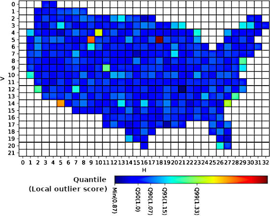
The rapid quality assessment approach was applied when the LCMAP products were first generated for the East mega ecoregion (Figure 3). Most of the tiles showed LOS less than 1.22, while two coastal tiles (H27V18 at West Palm Beach, Florida, and H26V20 at Key West, Florida) were above 2 (Figure 3). The primary land cover confidence map showed that the two tiles did not have time series models saved at the land pixels, and LCMAP land cover classes were filled using the translated NLCD 2001 map (Figure 4). The high LOS suggested the approach successfully identified these problematic tiles.
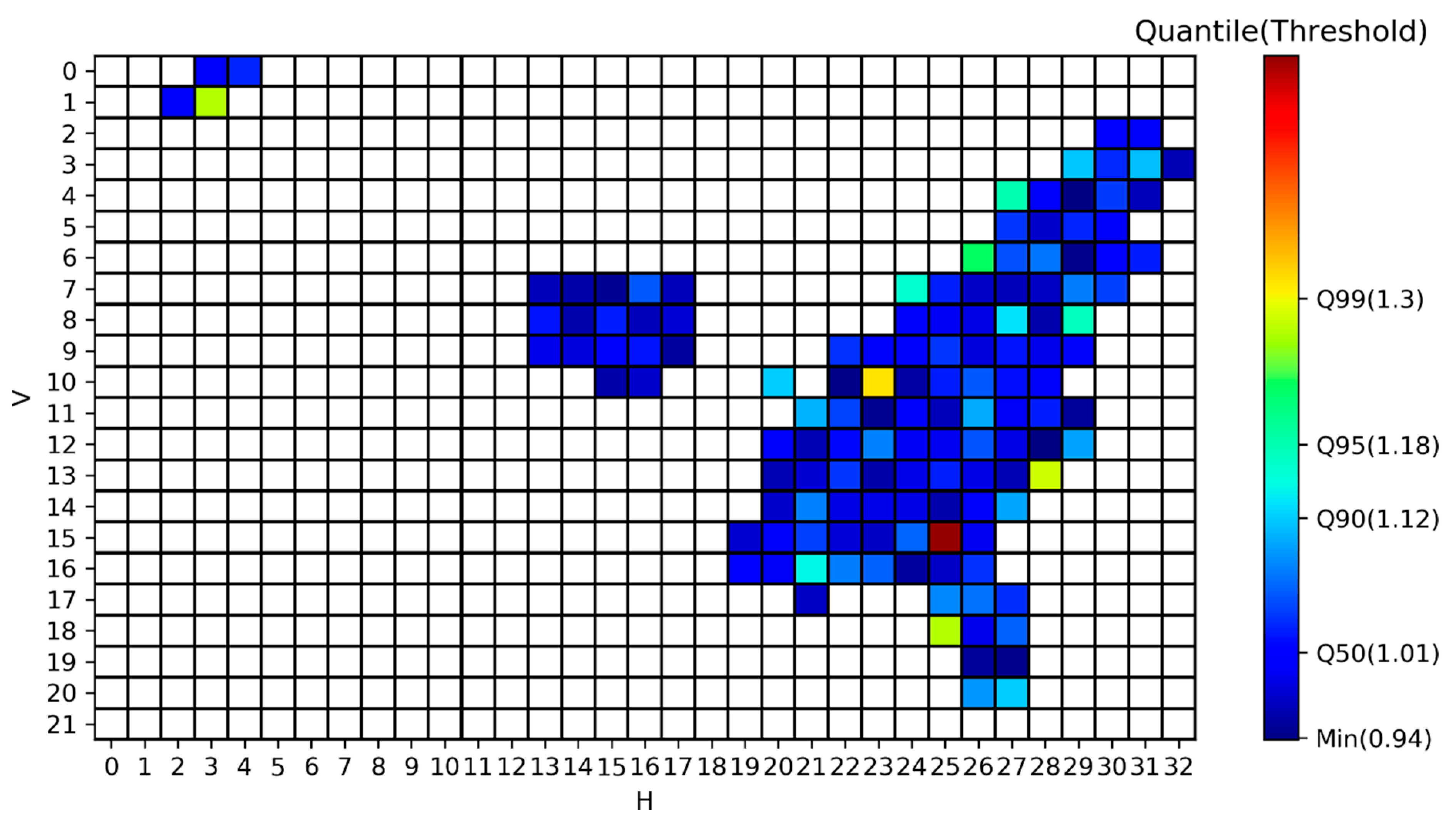
The problematic tiles successfully identified in West Palm Beach and Key West were later reproduced. Figure 5 shows the LOS values of H27V18 and H26V20 were reduced to 1.06 and 1.09, respectively, while the maximum LOS (1.5) came from tile H25V15. The indices suggested tile H25V15 had the smallest cohesive disagreement pixels with NLCD, but the highest SCTIME maximum, mean, and standard deviation (Table 3). A comparison of the LCMAP and NLCD land cover products showed that the primary disagreement came from the fragmented tree or grass-shrub (Figure 6). Both LCMAP and NLCD indicated this tile had intensive forest harvest activities, while trees in this region only took about 6 years to grow back. Thus, a possible reason for the disagreement is that NLCD often searches surrounding years of Landsat images for clear observations, which could cause the temporal shift of the tree regrowth estimation in NLCD. Moreover, the Okefenokee Swamp (across Georgia and Florida) in tile H25V15 had two large fires in 2007 and 2011 [43], which resulted in a distinctive annual change rate (Figure 7).
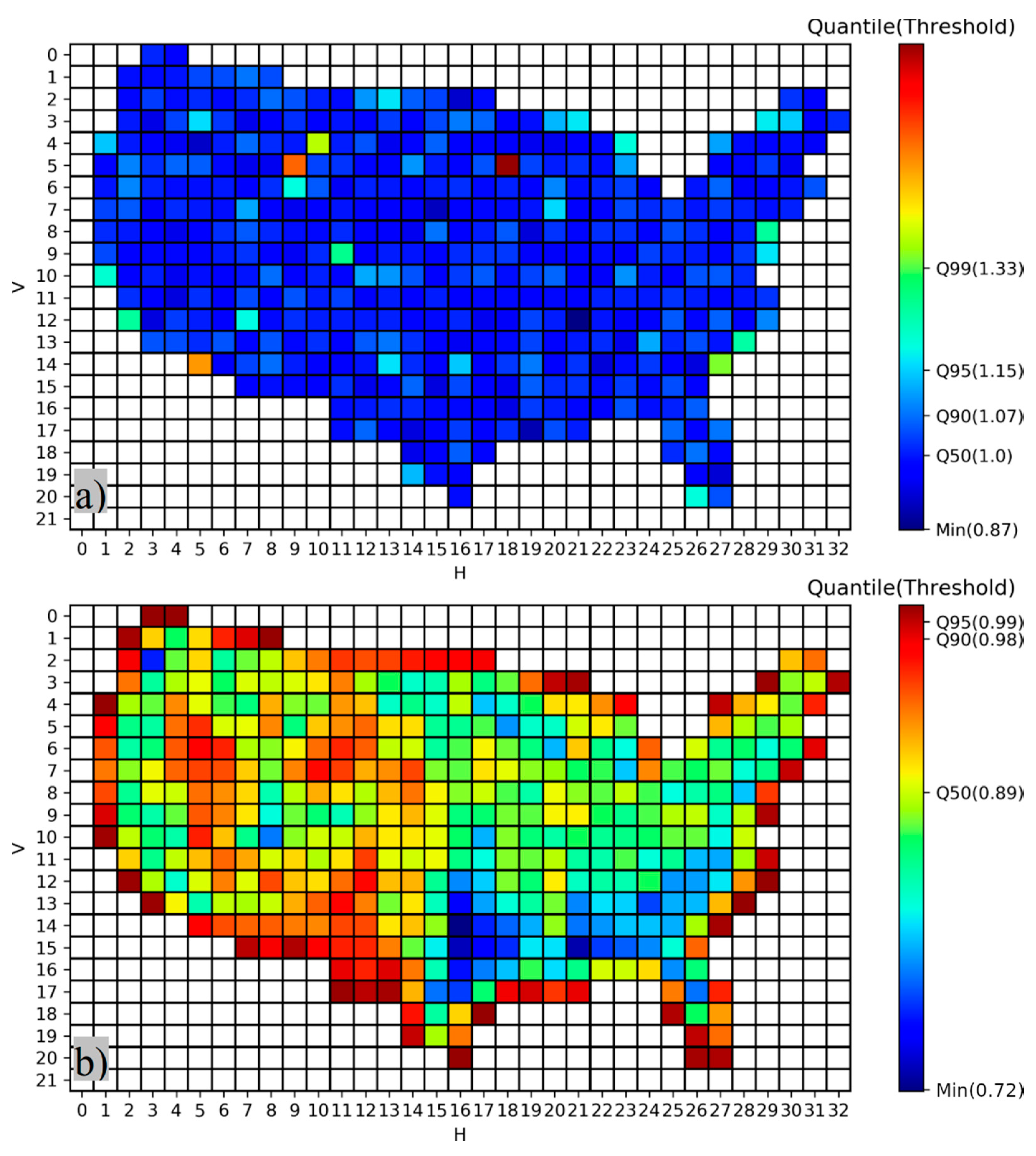
Figure 8a shows the final LOS map for the whole CONUS. The lowest agreement between the NLCD and LCMAP land cover products was at least 71.5% and averaged 89.1% (Figure 8b). The coasts and borders show high agreement between the two products because they are dominated by water bodies. The average and median LOS were both 1.0, while the maximum LOS was 1.72 at H18V05. According to Table 4, H18V05 had the lowest agreement with NLCD (79.3%), the highest single pixels with no model initialized, and the highest SCTIME maximum, mean, and standard deviation. However, compared to H25V15, tile H18V05 had much lower SCTIME and LC Change indices (Table 3 and Table 4), which means land cover in H18V05 was much more stable. The primary disagreement between LCMAP and NLCD in tile H18V05 was woody wetland in NLCD, but tree cover in LCMAP (Figure 9). The disagreement is a result of the differences in classification methods. NLCD used hierarchical classification and integration, which assigned higher priority to wetland cover than forest [44]. In contrast, LCMAP relied mainly on the seasonal variation of surface reflectance, in which woody wetland and trees are similar. Changes were detected in many wetlands in this tile for 1990, but the cover type remained the same in 1991 for most of those pixels, which resulted in a high spike in the annual spectral change rate (Figure 10a) but moderate land cover change rate (Figure 10b). Another reason for the distinction of H18V05 is the metropolitan area (Minneapolis and St. Paul) that covers a large portion of tile H18V05 and is the only metropolitan area in the 3 by 3 tile grid. The highest land cover change rate occurred in 1988, and the most common change type was the conversion from cropland to developed, which mainly occurred in the southeastern part of Minneapolis and St. Paul, Minnesota, along the Mississippi River.
Traditional product quality control activities were based on export interpretation [35,36,45] or validation after the production was completed [37,38]. Most validation methods involve elements of sampling design, land cover identification, and accuracy assessment [39,40]. However, it was impractical for interpreters to evaluate the massive amount of data during production, and inefficient to reproduce the whole product if we rely only on the final validation. This study presents a workflow to consistently, automatically, and rapidly assess the quality of LCMAP results during production. We assessed the stability of LCMAP products both spatially and temporally. While multiple years of NLCD land cover maps were used to ensure that the overall results were consistent with existing products, the temporal stability was estimated for both land cover and change products. We removed the road network from the translated NLCD classes to reduce potential mismatches. This is because NLCD embedded the road features after the land cover classification from a non-remote sensing source, while we focus on the agreement between the classification results of the two products. This study does not provide a statistical validation of the LCMAP land cover results using NLCD products. Any disagreement between the two land-cover datasets does not necessarily indicate an error in the LCMAP results. For the purpose of validation, LCMAP has developed an independent reference dataset at the national level to validate the final products [37]. The rapid quality assessments discussed here were conducted for each ARD tile and results were compared with the surrounding tiles to identify anomalous tiles. In the simulated data tests, we found that tiles with random noises have LOS higher than 2, given the 14 indices. Thus, we use the threshold 2 as a flag for erroneous tiles. However, when all tiles have a LOS lower than the threshold, we still evaluate tiles with relatively high LOS to ensure the quality of the product. The approach successfully detected erroneous tiles during production and provided auxiliary information for future investigation to remedy the problems.
The comparison procedure integrated multiple independent indices that can be easily adjusted to meet future concerns. The method developed for evaluating LCMAP products in a rapid manner could be useful for other time series land cover change-related research and large-scale applications. However, users should be aware of some limitations of the method. One limitation is that the LOS is hard to interpret in order to decide the threshold of the outlier. Thus, instead of relying on the threshold, we use the LOS as a guide in evaluating tiles with a relatively high score. Another solution is the extension of the local outlier factor analysis, which scaled the LOS to a value range of [0:1]. The result is directly interpretable as a probability of outlier. Another limitation is that this workflow only flags outlier tiles with potential hardware or software failure, rather than algorithm deficiency. For example, if the algorithm had lower accuracy in the 1980s for all tiles, the workflow would not derive high LOS related to the problem. Thus, the approach should not be used as an accuracy assessment. For the LCMAP project, an independent validation study was conducted to estimate the annual land cover and change accuracy [41].
5. Conclusions
In this paper, we described a procedure for automatically and rapidly monitoring the quality of extensive results during the production of land cover and land surface change products. We developed methods involving 14 indices to assess the stability of LCMAP products, both spatially and temporally. The 14 indices allow us to find and flag potential anomalous tiles in the suite of 10 LCMAP products by comparing them with neighboring tiles using local outlier analysis. The methods successfully identified erroneous results from the simulated data and during the LCMAP production, in which erroneous tiles had LOS greater than 2. The calculated indices also suggest directions for further investigation of anomalous tiles. The local outlier analysis is flexible to input indices, which allows us to extend the indices’ metrics for distinct characteristics, such as land cover change patterns or consistency with existing products. Our results showed all LOS values are below 2 in the final products, and overall agreements between LCMAP and NLCD are at least 71.5% and average 89.1%. A large volume of land cover data available globally is a significant benefit for ecosystem study and environmental management. However, quickly assessing production quality is challenging. Our approach offers the potential to automatically evaluate product quality from the perspective of multiple characteristics.
Author Contributions
Conceptualization, G.X.; methodology, Q.Z., C.B.; supervision, G.X.; writing—original draft, Q.Z.; writing—review and editing, G.X. All authors have read and agreed to the published version of the manuscript.
Funding
This research was funded by the USGS National Land Imaging (NLI) program under contract 140G0119C0001.
Acknowledgments
We thank Jesslyn Brown, Matthew Rigge, Thomas Adamson, Sandra Cooper, the academic editor and the anonymous reviewers who helped us substantially improve the manuscript.
Conflicts of Interest
The authors declare no conflict of interest.
Statement
Any use of trade, firm, or product names is for descriptive purposes only and does not imply endorsement by the U.S. Government.
References
- Rindfuss, R.R.; Walsh, S.J.; Turner Ii, B.L.; Fox, J.; Mishra, V. Developing a science of land change: Challenges and methodological issues. Proc. Natl. Acad. Sci. USA 2004, 101, 13976–13981. [Google Scholar]
- Wulder, M.A.; Coops, N.C.; Roy, D.P.; White, J.C.; Hermosilla, T. Land cover 2.0. Int. J. Remote Sens. 2018, 39, 4254–4284. [Google Scholar]
- Achard, F.; Eva, H.D.; Mayaux, P.; Stibig, H.J.; Belward, A. Improved estimates of net carbon emissions from land cover change in the tropics for the 1990s. Glob. Biogeochem. Cycles 2004, 18, GB2008. [Google Scholar]
- Houghton, R.A.; House, J.I.; Pongratz, J.; van der Werf, G.R.; DeFries, R.S.; Hansen, M.C.; Le Quéré, C.; Ramankutty, N. Carbon emissions from land use and land-cover change. Biogeosciences 2012, 9, 5125–5142. [Google Scholar]
- Tan, Z.; Liu, S.; Sohl, T.L.; Wu, Y.; Young, C.J. Ecosystem carbon stocks and sequestration potential of federal lands across the conterminous United States. Proc. Natl. Acad. Sci. USA 2015, 112, 12723–12728. [Google Scholar]
- Wu, Y.; Liu, S.; Tan, Z. Quantitative attribution of major driving forces on soil organic carbon dynamics. J. Adv. Model. Earth Syst. 2015, 7, 21–34. [Google Scholar]
- Senay, G.B.; Friedrichs, M.; Singh, R.K.; Velpuri, N.M. Evaluating Landsat 8 evapotranspiration for water use mapping in the Colorado River Basin. Remote Sens. Environ. 2016, 185, 171–185. [Google Scholar]
- Stow, D.A.; Hope, A.; McGuire, D.; Verbyla, D.; Gamon, J.; Huemmrich, F.; Houston, S.; Racine, C.; Sturm, M.; Tape, K.; et al. Remote sensing of vegetation and land-cover change in Arctic Tundra Ecosystems. Remote Sens. Environ. 2004, 89, 281–308. [Google Scholar]
- Hansen, M.C.; Potapov, P.V.; Moore, R.; Hancher, M.; Turubanova, S.A.; Tyukavina, A.; Thau, D.; Stehman, S.V.; Goetz, S.J.; Loveland, T.R.; et al. High-resolution global maps of 21st-century forest cover change. Science 2013, 342, 850–853. [Google Scholar]
- Kennedy, R.E.; Andrefouet, S.; Cohen, W.B.; Gomez, C.; Griffiths, P.; Hais, M.; Healey, S.P.; Helmer, E.H.; Hostert, P.; Lyons, M.B.; et al. Bringing an ecological view of change to Landsat-based remote sensing. Front. Ecol. Environ. 2014, 12, 339–346. [Google Scholar]
- Masek, J.G.; Huang, C.; Wolfe, R.; Cohen, W.; Hall, F.; Kutler, J.; Nelson, P. North American forest disturbance mapped from a decadal Landsat record. Remote Sens. Environ. 2008, 112, 2914–2926. [Google Scholar]
- Liu, H.; Zhan, Q.; Gao, S.; Yang, C. Seasonal variation of the spatially non-stationary association between land surface temperature and urban landscape. Remote Sens. 2019, 11, 1016. [Google Scholar]
- He, B.; Zhao, Z.; Shen, L.; Wang, H.; Li, L. An approach to examining performances of cool/hot sources in mitigating/enhancing land surface temperature under different temperature backgrounds based on landsat 8 image. Sustain. Cities Soc. 2019, 44, 416–427. [Google Scholar]
- Fu, P.; Weng, Q. A time series analysis of urbanization induced land use and land cover change and its impact on land surface temperature with Landsat imagery. Remote Sens. Environ. 2016, 175, 205–214. [Google Scholar]
- Latifovic, R.; Pouliot, D. Multitemporal land cover mapping for Canada: Methodology and products. Can. J. Remote Sens. 2005, 31, 347–363. [Google Scholar]
- Olthof, I.; Latifovic, R.; Pouliot, D. Medium Resolution Land Cover Mapping of Canada from SPOT 4/5 Data. Geomatics Canada, Open File 4. 2015. Available online: http://ftp2.cits.rncan.gc.ca/pub/geott/ess_pubs/295/295751/of_0004_gc.pdf (accessed on 10 July 2020).
- da Campos Macedo, R.; Moreira, M.Z.; Domingues, E.; Couto, Â.M.R.; da Giusti Sanson, F.E.; Teixeira, F.W. LUCC (Land Use and Cover Change) and the environmental-economic accounts system in Brazil. J. Earth Sci. Eng. 2013, 3, 840. [Google Scholar]
- Prodes, I.P. Monitoramento da floresta Amazônica Brasileira por satélite. Inst. Nac. Pesqui. Espac. Proj. Prodes. 2013, 25, 2013. [Google Scholar]
- Lymburner, L.; Tan, P.; McIntyre, A.; Lewis, A.; Thankappan, M. Dynamic Land Cover Dataset version 2: 2001-now…a land cover odyssey. In Proceedings of the 2013 IEEE International Geoscience and Remote Sensing Symposium-IGARSS, Melbourne, Australia, 21–26 July 2013. [Google Scholar]
- Deng, X.; Liu, J. Mapping land cover and land use changes in China. In Remote Sensing of Land Use and Land Cover: Principles and Applications; CRC Press: Boca Raton, FL, USA, 2012; pp. 339–349. [Google Scholar]
- Hu, L.; Chen, Y.; Xu, Y.; Zhao, Y.; Yu, L.; Wang, J.; Gong, P. A 30 meter land cover mapping of China with an efficient clustering algorithm CBEST. Sci. China Earth Sci. 2014, 57, 2293–2304. [Google Scholar]
- Feranec, J.; Soukup, T.; Hazeu, G.; Jaffrain, G. (Eds.) European Landscape Dynamics: CORINE Land Cover Data; CRC Press: Boca Raton, FL, USA, 2016. [Google Scholar]
- Inglada, J.; Vincent, A.; Arias, M.; Tardy, B.; Morin, D.; Rodes, I. Operational high resolution land cover map production at the country scale using satellite image time series. Remote Sens. 2017, 9, 95. [Google Scholar]
- Schepaschenko, D.; McCallum, I.; Shvidenko, A.; Fritz, S.; Kraxner, F.; Obersteiner, M. A new hybrid land cover dataset for Russia: A methodology for integrating statistics, remote sensing and in situ information. J. Land Use Sci. 2011, 6, 245–259. [Google Scholar]
- Pekel, J.F.; Cottam, A.; Gorelick, N.; Belward, A.S. High-resolution mapping of global surface water and its long-term changes. Nature 2016, 540, 418–422. [Google Scholar]
- Xiong, J.; Thenkabail, P.S.; Tilton, J.C.; Gumma, M.K.; Teluguntla, P.; Oliphant, A.; Congalton, R.G.; Yadav, K.; Gorelick, N. Nominal 30-m cropland extent map of continental Africa by integrating pixel-based and object-based algorithms using Sentinel-2 and Landsat-8 data on Google Earth Engine. Remote Sens. 2017, 9, 1065. [Google Scholar]
- Loveland, T.R.; Reed, B.C.; Brown, J.F.; Ohlen, D.O.; Zhu, Z.; Yang, L.; Merchant, J.W. Development of a global land cover characteristics database and IGBP DISCover from 1 km AVHRR data. Int. J. Remote Sens. 2000, 21, 1303–1330. [Google Scholar]
- Homer, C.G.; Dewitz, J.A.; Yang, L.; Jin, S.; Danielson, P.; Xian, G.; Coulston, J.; Herold, N.D.; Wickham, J.D.; Megown, K. Completion of the 2011 National Land Cover Database for the conterminous United States–representing a decade of land cover change information. Photogramm. Eng. Remote Sens. 2015, 81, 345–354. [Google Scholar]
- Homer, C.; Dewitz, J.; Fry, J.; Coan, M.; Hossain, N.; Larson, C.; Herold, N.; McKerrow, A.; VanDriel, J.N.; Wickham, J. Completion of the 2001 national land cover database for the counterminous United States. Photogramm. Eng. Remote Sens. 2007, 73, 337. [Google Scholar]
- Yang, L.; Jin, S.; Danielson, P.; Homer, C.; Gass, L.; Bender, S.M.; Case, A.; Costello, C.; Dewitz, J.; Fry, J.; et al. A new generation of the United States National Land Cover Database: Requirements, research priorities, design, and implementation strategies. ISPRS J. Photogramm. Remote Sens. 2018, 146, 108–123. [Google Scholar]
- Turner, B.L.; Lambin, E.F.; Reenberg, A. The emergence of land change science for global environmental change and sustainability. Proc. Natl. Acad. Sci. USA 2007, 104, 20666–20671. [Google Scholar]
- Brown, J.F.; Tollerud, H.J.; Barber, C.P.; Zhou, Q.; Dwyer, J.L.; Vogelmann, J.E.; Loveland, T.R.; Woodcock, C.E.; Stehman, S.V.; Zhu, Z. Lessons learned implementing an operational continuous United States national land change monitoring capability: The Land Change Monitoring, Assessment, and Projection (LCMAP) approach. Remote Sens. Environ. 2019, 238, 111356. [Google Scholar]
- Dwyer, J.L.; Roy, D.P.; Sauer, B.; Jenkerson, C.B.; Zhang, H.K. Analysis ready data: Enabling analysis of the Landsat archive. Remote Sens. 2018, 10, 1363. [Google Scholar]
- Zhu, Z.; Woodcock, C.E. Continuous change detection and classification of land cover using all available Landsat data. Remote Sens. Environ. 2014, 144, 152–171. [Google Scholar]
- Carfagna, E.; Marzialetti, J. Sequential design in quality control and validation of land cover databases. Appl. Stoch. Models Bus. Ind. 2009, 25, 195–205. [Google Scholar]
- Estima, J.; Painho, M. Photo based Volunteered Geographic Information initiatives: A comparative study of their suitability for helping quality control of Corine Land Cover. In Geospatial Intelligence: Concepts, Methodologies, Tools, and Applications; IGI Global: Hershey, PA, USA, 2019; pp. 1124–1142. [Google Scholar]
- Wu, W.; Shibasaki, R.; Ongaro, L.; Ongaro, L.; Zhou, Q.; Tang, H. Validation and comparison of 1 km global land cover products in China. Int. J. Remote Sens. 2008, 29, 3769–3785. [Google Scholar]
- Stehman, S.V.; Olofsson, P.; Woodcock, C.E.; Herold, M.; Friedl, M.A. A global land-cover validation data set, II: Augmenting a stratified sampling design to estimate accuracy by region and land-cover class. Int. J. Remote Sens. 2012, 33, 6975–6993. [Google Scholar]
- Strahler, A.H.; Boschetti, L.; Foody, G.M.; Friedl, M.A.; Hansen, M.C.; Herold, M.; Mayaux, P.; Morisette, J.; Stehman, S.V.; Woodcock, C.E. Global Land Cover Validation: Recommendations for Evaluation and Accuracy Assessment of Global Land Cover Maps; European Communities: Luxembourg, 2006; p. 51. [Google Scholar]
- Olofsson, P.; Stehman, S.V.; Woodcock, C.E.; Sulla-Menashe, D.; Sibley, A.M.; Newell, J.D.; Friedl, M.A.; Herold, M. A global land-cover validation data set, part I: Fundamental design principles. Int. J. Remote Sens. 2012, 33, 5768–5788. [Google Scholar]
- Pengra, B.W.; Stehman, S.V.; Horton, J.A.; Dockter, D.J.; Schroeder, T.A.; Yang, Z.; Cohen, W.B.; Healey, S.P.; Loveland, T.R. Quality control and assessment of interpreter consistency of annual land cover reference data in an operational national monitoring program. Remote Sens. Environ. 2019, 238, 111261. [Google Scholar]
- Xian, G.; Homer, C.; Fry, J. Updating the 2001 National Land Cover Database land cover classification to 2006 by using Landsat imagery change detection methods. Remote Sens. Environ 2009, 113, 1133–1147. [Google Scholar]
- Eidenshink, J.; Schwind, B.; Brewer, K.; Zhu, Z.-L.; Quayle, B.; Howard, S. A project for monitoring trends in burn severity. Fire Ecol. 2007, 3, 3–21. [Google Scholar]
- Jin, S.; Homer, C.; Yang, L.; Danielson, P.; Dewitz, J.; Li, C.; Zhu, Z.; Xian, G.; Howard, D. Overall Methodology Design for the United States National Land Cover Database 2016 Products. Remote Sens. 2019, 11, 2971. [Google Scholar]
- Kriegel, H.P.; Kröger, P.; Schubert, E.; Zimek, A. LoOP: Local outlier probabilities. In Proceedings of the 18th ACM Conference on Information and Knowledge Management, Hong Kong, China, 2–6 November 2009. [Google Scholar]
Figure 1.
Illustration of land cover types in one tile (150 km by 150 km) at panel (a), and synthetic data with 5% failed pixels (black color) at panel (b) or 15% failed pixels at panel (c). The lower-left corner of each panel displays the zoom-in view of the image center.
Figure 1.
Illustration of land cover types in one tile (150 km by 150 km) at panel (a), and synthetic data with 5% failed pixels (black color) at panel (b) or 15% failed pixels at panel (c). The lower-left corner of each panel displays the zoom-in view of the image center.

Figure 2.
Local outlier scores estimated for synthetic data with random pixels failed in one year (left) or all years (right).
Figure 2.
Local outlier scores estimated for synthetic data with random pixels failed in one year (left) or all years (right).

Figure 3.
Illustration of outlier detection results during the first production. The color bar shows LOS value at the 50%, 90%, 95%, and 99% cut points. X and y axes show horizontal (H) and vertical (V) tile number, respectively.
Figure 3.
Illustration of outlier detection results during the first production. The color bar shows LOS value at the 50%, 90%, 95%, and 99% cut points. X and y axes show horizontal (H) and vertical (V) tile number, respectively.

Figure 4.
The primary land cover confidence of two outlier tiles. Red means no stable time series models were produced for this pixel, so the land cover classes of translated NLCD 2001 were used. Cyan represents the ocean.
Figure 4.
The primary land cover confidence of two outlier tiles. Red means no stable time series models were produced for this pixel, so the land cover classes of translated NLCD 2001 were used. Cyan represents the ocean.

Figure 5.
Illustration of outlier detection results after the reproduction. The color bar shows LOS value at the 50%, 90%, 95%, and 99% cut points. X and y axes show horizontal (H) and vertical (V) tile number, respectively.
Figure 5.
Illustration of outlier detection results after the reproduction. The color bar shows LOS value at the 50%, 90%, 95%, and 99% cut points. X and y axes show horizontal (H) and vertical (V) tile number, respectively.

Figure 6.
Example of the LCMAP and NLCD products at tile H25V15 in corresponding years: (a) LCMAP-2001; (b) NLCD-2001; (c) difference between LCMAP and NLCD in 2001; (d) LCMAP-2006; (e) NLCD-2006; (f) difference between LCMAP and NLCD in 2006; (g) LCMAP-2011; (h) NLCD-2011; (i) difference between LCMAP and NLCD in 2011. The major land cover classes include Tree (green), Wetland (light blue), Grass/Shrub (yellow), Developed (red), and Cropland (brown).

Figure 7.
The (a) annual change rate and (b) annual land cover change rate of H25V15 (red line) compared to the neighboring tiles (black lines).
Figure 7.
The (a) annual change rate and (b) annual land cover change rate of H25V15 (red line) compared to the neighboring tiles (black lines).

Figure 8.
Illustration of outlier detection results for the final production (a). Panel (b) shows the lowest level of agreement between LCMAP and NLCD in 2001, 2006, or 2011. X and y axes show horizontal (H) and vertical (V) tile number, respectively.
Figure 8.
Illustration of outlier detection results for the final production (a). Panel (b) shows the lowest level of agreement between LCMAP and NLCD in 2001, 2006, or 2011. X and y axes show horizontal (H) and vertical (V) tile number, respectively.

Figure 9.
Example of the LCMAP and NLCD products at tile H18V05 in corresponding years: (a) LCMAP-2001; (b) NLCD-2001; (c) difference between LCMAP and NLCD in 2001; (d) LCMAP-2006; (e) NLCD-2006; (f) difference between LCMAP and NLCD in 2006; (g) LCMAP-2011; (h) NLCD-2011; (i) difference between LCMAP and NLCD in 2011. The major land cover classes include Tree (green), Wetland (light blue), Water (dark blue), Grass/Shrub (yellow), Developed (red), and Cropland (brown).

Figure 10.
The (a) annual change rate and (b) annual land cover change rate for H18V05 (red line) compared to the neighboring tiles (black lines).
Figure 10.
The (a) annual change rate and (b) annual land cover change rate for H18V05 (red line) compared to the neighboring tiles (black lines).


Table 1.
The translation from NLCD to LCMAP classes. Values in parentheses are the land cover class code.
Table 1.
The translation from NLCD to LCMAP classes. Values in parentheses are the land cover class code.
| NLCD Class (Class Code) | LCMAP Class (Class Code) |
|---|---|
| Water (11) | Water (5) |
| Perennial ice/snow (12) | Ice and Snow (7) |
| Developed, open space (21) | Developed (1) |
| Developed, low intensity (22) | Developed (1) |
| Developed, medium intensity (23) | Developed (1) |
| Developed, high intensity (24) | Developed (1) |
| Barren (31) | Barren (8) |
| Deciduous forest (41) | Tree Cover (4) |
| Evergreen forest (42) | Tree Cover (4) |
| Mixed forest (43) | Tree Cover (4) |
| Shrubland (52) | Grass/shrub (3) |
| Grassland (71) | Grass/shrub (3) |
| Pasture (81) | Cropland (2) |
| Cultivated crops (82) | Cropland (2) |
| Woody wetlands (90) | Wetland (6) |
| Herbaceous wetland (95) | Wetland (6) |
Table 2.
List of indices for each tile to characterize the reasonableness of LCMAP products in both spatial and temporal directions.
Table 2.
List of indices for each tile to characterize the reasonableness of LCMAP products in both spatial and temporal directions.
| INDEX | DESCRIPTION |
|---|---|
| Least agreement | The least agreement between NLCD and LCMAP in 2001, 2006, and 2011. |
| Disagreement large patch | Largest size of cohesive pixels that disagree between NLCD and LCMAP in 2001, 2006, and 2011. |
| Disagreement salt pepper | Number of single pixels that disagree between NLCD and LCMAP in 2001, 2006, and 2011. |
| No model large patch | Largest size of cohesive pixels that have insufficient observation to initialize model. |
| No model salt pepper | Number of single pixels that have insufficient observation to initialize model. |
| Urban decrease | Maximum urban area decreases in 30+ years. |
| SCTIME max | Maximum annual spectral change rate across time series of the Timing of Spectral Change product (SCTIME). |
| SCTIME mean | Mean annual change spectral rate across time series. |
| SCTIME min | Minimum annual change spectral rate across time series. |
| SCTIME std | Standard deviation annual spectral change rate across time series. |
| LC Change max | Maximum annual land cover change rate across time series. |
| LC Change mean | Mean annual land cover change rate across time series. |
| LC Change min | Minimum annual land cover change rate across time series. |
| LC Change std | Standard deviation annual land cover change rate across time series. |
Table 3.
Results of indices for H25V15 and its neighboring tiles.
| Tile | H25V15 | H24V14 | H24V15 | H24V16 | H25V14 | H25V16 | H26V14 | H26V15 | H26V16 | |
|---|---|---|---|---|---|---|---|---|---|---|
| Least agreement | 82.6% | 80.5% | 78.9% | 90.8% | 79.9% | 79.0% | 88.2% | 94.4% | 85.5% | |
| Disagreement (km2) | large patch | 1.37 | 1.53 | 4.23 | 3.81 | 1.38 | 4.12 | 4.26 | 3.29 | 4.32 |
| salt pepper | 170.50 | 159.48 | 154.56 | 93.01 | 184.40 | 163.02 | 117.25 | 56.42 | 109.49 | |
| No model (km2) | large patch | 0.28 | 0.13 | 0.20 | 0.58 | 0.23 | 0.56 | 0.14 | 0.76 | 1.19 |
| salt pepper | 0.97 | 2.42 | 0.66 | 3.20 | 1.59 | 2.29 | 1.56 | 7.68 | 8.13 | |
| Urban decrease (km2) | 10.96 | 57.18 | 24.35 | 2.56 | 111.89 | 23.16 | 14.18 | 7.55 | 14.42 | |
| SCTIME | max | 0.125 | 0.074 | 0.071 | 0.066 | 0.071 | 0.093 | 0.056 | 0.066 | 0.084 |
| mean | 0.057 | 0.037 | 0.034 | 0.035 | 0.049 | 0.052 | 0.036 | 0.041 | 0.041 | |
| min | 0.009 | 0.003 | 0.004 | 0.005 | 0.011 | 0.004 | 0.009 | 0.011 | 0.006 | |
| std | 0.025 | 0.013 | 0.013 | 0.012 | 0.015 | 0.020 | 0.011 | 0.013 | 0.016 | |
| LC Change | max | 0.038 | 0.034 | 0.028 | 0.022 | 0.035 | 0.042 | 0.024 | 0.031 | 0.033 |
| mean | 0.028 | 0.025 | 0.018 | 0.016 | 0.028 | 0.032 | 0.017 | 0.023 | 0.023 | |
| min | 0.014 | 0.012 | 0.010 | 0.006 | 0.017 | 0.014 | 0.012 | 0.016 | 0.012 | |
| std | 0.004 | 0.004 | 0.004 | 0.003 | 0.004 | 0.006 | 0.002 | 0.003 | 0.004 |
Table 4.
Results of indices for H18V05 and its neighbor tiles.
| Tile | H18V5 | H17V4 | H17V5 | H17V6 | H18V4 | H18V6 | H19V4 | H19V5 | H19V6 | |
|---|---|---|---|---|---|---|---|---|---|---|
| Least agreement | 79.3% | 80.5% | 86.8% | 90.1% | 83.0% | 87.2% | 86.4% | 83.0% | 85.4% | |
| Disagreement (km2) | large patch | 5.43 | 6.25 | 6.21 | 1.91 | 5.13 | 5.10 | 4.43 | 5.19 | 2.98 |
| salt_pepper | 134.93 | 118.20 | 79.46 | 55.61 | 154.00 | 84.46 | 77.35 | 130.14 | 169.88 | |
| No model (km2) | large patch | 0.34 | 0.19 | 0.25 | 0.13 | 0.26 | 0.39 | 0.83 | 0.62 | 0.51 |
| salt_pepper | 6.81 | 1.82 | 2.03 | 1.63 | 1.11 | 4.42 | 2.20 | 5.05 | 3.21 | |
| Urban decrease (km2) | 0.37 | 2.17 | 5.21 | 9.67 | 0.18 | 0.27 | 1.33 | 1.20 | 3.52 | |
| SCTIME | max | 0.024 | 0.010 | 0.010 | 0.009 | 0.014 | 0.013 | 0.007 | 0.006 | 0.005 |
| mean | 0.007 | 0.005 | 0.004 | 0.002 | 0.005 | 0.003 | 0.004 | 0.003 | 0.003 | |
| min | 0.000 | 0.001 | 0.000 | 0.000 | 0.001 | 0.000 | 0.001 | 0.000 | 0.000 | |
| std | 0.005 | 0.002 | 0.002 | 0.002 | 0.003 | 0.002 | 0.001 | 0.001 | 0.001 | |
| LC Change | max | 0.007 | 0.002 | 0.003 | 0.002 | 0.003 | 0.003 | 0.003 | 0.002 | 0.002 |
| mean | 0.003 | 0.001 | 0.001 | 0.001 | 0.002 | 0.001 | 0.002 | 0.001 | 0.001 | |
| min | 0.001 | 0.001 | 0.000 | 0.000 | 0.001 | 0.000 | 0.001 | 0.001 | 0.001 | |
| std | 0.001 | 0.000 | 0.001 | 0.000 | 0.001 | 0.000 | 0.001 | 0.000 | 0.000 |
© 2020 by the authors. Licensee MDPI, Basel, Switzerland. This article is an open access article distributed under the terms and conditions of the Creative Commons Attribution (CC BY) license (http://creativecommons.org/licenses/by/4.0/).
Share and Cite
MDPI and ACS Style
Zhou, Q.; Barber, C.; Xian, G. Methods of Rapid Quality Assessment for National-Scale Land Surface Change Monitoring. Remote Sens. 2020, 12, 2524. https://doi.org/10.3390/rs12162524
AMA Style
Zhou Q, Barber C, Xian G. Methods of Rapid Quality Assessment for National-Scale Land Surface Change Monitoring. Remote Sensing. 2020; 12(16):2524. https://doi.org/10.3390/rs12162524
Chicago/Turabian StyleZhou, Qiang, Christopher Barber, and George Xian. 2020. "Methods of Rapid Quality Assessment for National-Scale Land Surface Change Monitoring" Remote Sensing 12, no. 16: 2524. https://doi.org/10.3390/rs12162524
Note that from the first issue of 2016, this journal uses article numbers instead of page numbers. See further details here.