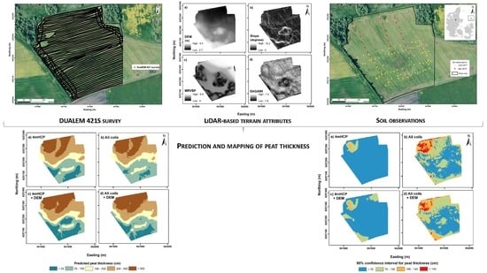
Mapping of Peat Thickness Using a Multi-Receiver Electromagnetic Induction Instrument


Department of Agroecology, Aarhus University, 8830 Tjele, Denmark
*
Author to whom correspondence should be addressed.
Remote Sens. 2020, 12(15), 2458; https://doi.org/10.3390/rs12152458
Submission received: 29 June 2020
/
Revised: 24 July 2020
/
Accepted: 30 July 2020
/
Published: 31 July 2020
(This article belongs to the Special Issue Estimation and Mapping of Soil Properties Based on Multi-Source Data Fusion)
Abstract
:Peatlands constitute extremely valuable areas because of their ability to store large amounts of soil organic carbon (SOC). Investigating different key peat soil properties, such as the extent, thickness (or depth to mineral soil) and bulk density, is highly relevant for the precise calculation of the amount of stored SOC at the field scale. However, conventional peat coring surveys are both labor-intensive and time-consuming, and indirect mapping methods based on proximal sensors appear as a powerful supplement to traditional surveys. The aim of the present study was to assess the use of a non-invasive electromagnetic induction (EMI) technique as an augmentation to a traditional peat coring survey that provides localized and discrete measurements. In particular, a DUALEM-421S instrument was used to measure the apparent electrical conductivity (ECa) over a 10-ha field located in Jutland, Denmark. In the study area, the peat thickness varied notably from north to south, with a range from 3 to 730 cm. Simple and multiple linear regressions with soil observations from 110 sites were used to predict peat thickness from (a) raw ECa measurements (i.e., single and multiple-coil predictions), (b) true electrical conductivity () estimates calculated using a quasi-three-dimensional inversion algorithm and (c) different combinations of ECa data with environmental covariates (i.e., light detection and ranging (LiDAR)-based elevation and derived terrain attributes). The results indicated that raw ECa data can already constitute relevant predictors for peat thickness in the study area, with single-coil predictions yielding substantial accuracies with coefficients of determination (R2) ranging from 0.63 to 0.86 and root mean square error (RMSE) values between 74 and 122 cm, depending on the measuring DUALEM-421S coil configuration. While the combinations of ECa data (both single and multiple-coil) with elevation generally provided slightly higher accuracies, the uncertainty estimates for single-coil predictions were smaller (i.e., smaller 95% confidence intervals). The present study demonstrates a high potential for EMI data to be used for peat thickness mapping.
1. Introduction
Under natural conditions, peatlands constitute carbon sinks. However, they have been used both for fuel mining and agriculture for over 1000 years. Climate change and rapid land use change have turned peatlands into carbon sources. Within the European Union 2030 climate and energy framework, all member states have to report on the emissions and removals of greenhouse gases from wetlands, including peatlands [1]. The assessment of key peat soil properties, such as the extent, thickness (or depth to mineral soil) and bulk density, is highly relevant for the precise calculation of the amount of stored soil organic carbon (SOC) at the field scale. Several methods have been used to measure peat thickness (or depth to mineral layer) in the field. Conventional measurements using hand augers are still commonly used, although this process is labor-intensive and time-consuming and only provides depth observations at single point locations. In different Digital Soil Mapping (DSM) studies, models were derived to predict peat thickness using conventional field observations and environmental data. Considering environmental data, a few studies mostly used terrain attributes, including elevation and slope [2,3], only elevation [4] or the distance to a river [5]. More recently, machine learning models have also been used [6,7,8] as well as regression kriging [9]. Rudiyanto et al. [6] (2016) and Young et al. [9] (2018) built models using a relatively limited amount of environmental data (i.e., elevation, slope, aspect, System of Automated Geoscientific Analyses Wetness Index (SAGAWI) and nearest distance to river for the first study, and elevation, slope, aspect, vegetation type and soil for the latter). Rudiyanto et al. [8] (2018) and Aitkenhead [7] (2017) used a wide array of environmental covariates: topography (i.e., elevation, vegetation-corrected elevation, and two derived terrain attributes—the Multi-Resolution Index of Valley Bottom Flatness (MRVBF) and SAGAWI—Euclidean distances to rivers, seas and combined rivers and seas, radar images (i.e., Sentinal-1A and ALOS-PALSAR) and vegetation (i.e., seven Landsat raw bands and the normalized difference vegetation index) in Rudiyanto et al. [8] (2018), and topography (i.e., elevation and seven derived terrain attributes), climate (i.e., 24 different meteorological layers), soil (i.e., land cover, geology and soil maps) and vegetation (i.e., Landsat raw bands and derived vegetation indices) in Aitkenhead [7] (2017).
Within soil sensing, geophysical techniques constitute a powerful supplement to traditional coring in the attempt to map peat properties at different scales. These methods cannot represent a complete alternative to field coring although they can significantly reduce costs by limiting the dependency on the latter only for calibration purposes. Peat displays particular electric properties, making geoelectric methods more suitable for mapping its thickness or extent. Its electrical conductivity depends mainly on the water content and amount of dissolved ions [10,11,12]). Peat also presents a high relative dielectric permittivity due to its generally high water content, which allows it to be distinguished from mineral soils with lower permittivity values [13]. Remote sensing and airborne geophysical techniques represent the most suitable means to investigate peatlands at a large scale (>10 km2). Several recent studies have successfully used airborne electromagnetic (AEM) methods to estimate peatland thickness and extent [14,15,16,17]. Likewise, different proximal or ground-based geophysical sensors have been accurately applied to map peat properties at smaller scales. Ground-penetrating radar (GPR) and electrical conductivity or resistivity surveys have been predominantly used to map peatlands [12]. In particular, GPR, which detects the contrast in dielectric permittivity, has been extensively used to map peat thickness for the last three decades [18,19,20,21,22]. Other studies have used complex electrical conductivity surveys [23] and electrical resistivity surveys [24] to explore the stratigraphy of peat. Electrical conductivity surveys based on electromagnetic induction (EMI) measure the apparent electrical conductivity (ECa) for a volume of soil. Recent advances in EMI technology have resulted in the advent of on-the-go sensing systems, making it possible to determine ECa for varying depths. ECa can further be used to determine true electrical conductivity () estimates from quasi-three-dimensional (quasi-3D) inversion models [25,26], thereby enabling the variation of soil properties in 3D to be inferred [27,28,29]. To our knowledge, EMI surveys have only been implemented in a few studies on peatlands: Theimer et al. [19] (1994) studied peat thickness, Slater and Reeve [21] (2002) investigated peatland stratigraphy and hydrology, Comas et al. [30] (2011) focused on peat basin morphology, and Koszinski et al. [31] (2015) and Altdorff et al. [32] (2016) estimated bulk density, SOC content and stock. Furthermore, a recent study by Boaga et al. [33] (2020) hypothesized that the combination of proximal and airborne electromagnetic data could be successfully used in a joint inversion scheme with the aim of enhancing the AEM survey resolution where ground-based EMI data are available and extending the results to larger areas where only AEM data might be available.
The aim of the present case study is to assess the use of data collected from a single-frequency multi-receiver EMI instrument—namely a DUALEM-421S—for the prediction of peat thickness. Soil observations were used for calibration and validation purposes. Linear regression (LR) and multiple linear regression (MLR) were used to investigate the spatial variability of peat thickness over a 10 ha field area located in Jutland, Denmark. This was done solely from ECa measurements (i.e., single and multiple-coil predictions) or from estimates calculated using a quasi-3D inversion algorithm and from the combination of ECa data with environmental covariates (i.e., topography variables comprising elevation and derived terrain attributes).
2. Materials and Methods
2.1. Study Area
The study area is a 10 ha agricultural field with a high peat thickness gradient (3–730 cm), located in the Nørre Å valley in central Jutland, Denmark (Figure 1). The field mainly comprises organic soil areas and small zones with mineral soils (coarse sand). This site is considered as a riparian fen peatland [34] where vascular plants such as reeds and sedges dominate [12]. As will be discussed later, and similar to Walter et al. [12] (2015), its specific configuration, underlain by sandy soils characterized by low electrical conductivity, ensured a contrast with the peat layers, which generally present higher electrical conductivity. The field belongs to the East Jutland glacial landscape and borders a young moraine landscape to the West [35]. The originally uneven tunnel-valley bottom has been covered by sea and organic sediments deposited after the last glaciation [36]. The study area is characterized by a temperate oceanic climate with a winter mean temperature of 0 °C and a summer mean temperature of 17 °C. The annual precipitation ranges from 650 to 750 mm [37]. The field is tile-drained and currently used as extensive grassland.
2.2. Soil Observations and Sampling Design
Soil observations were collected during two sampling survey campaigns in June 2017 and May 2019 (Figure 1). The thickness of peat deposits (or depth to the mineral layer) was investigated using a peat probe including a 120 cm main part and 94 cm extension rods. During the 2017 campaign, 76 soil observations were carried out following five pseudo-transects roughly in a southwest–northeast orientation. These first observations were restricted to the southern half of the study area as a plot experiment was running in the northern part. The locations were selected directly in the field using the results from a DUALEM-21S survey carried out at the same time. Preliminary ECa maps were generated using kriging within ArcMap [39]. During the 2019 campaign, 34 soil observations were carried out following three transects in a northwest–southeast orientation. Their locations were selected using preliminary kriged ECa maps from a recent DUALEM-421S survey (i.e., from April 2019). In total, 110 soil observations were used as calibration and validation data within the predictive modeling of peat thickness. The sampling approach can be compared to that recommended by Rudiyanto et al. [6] (2016), which was based on (1) stratifying the study area by elevation (in our case, kriged ECa data) and (2) sampling locations along transects crossing all strata or random locations within each stratum (in our case, along transects). The precise location of each soil observation was determined in the field using a conventional portable GPS system (Trimble SPS851 Global Navigation Satellite System, Trimble Navigation Limited, Sunnyvale, CA, USA).
2.3. DUALEM-421S Data Collection
An EMI instrument typically comprises a transmitter (Tx) and a receiver (Rx) coil. A primary magnetic field is generated by powering the Tx coil with an alternating current. This primary field creates eddy currents in the conductive media present in the subsurface inducing a secondary magnetic field. Both the primary and secondary fields are detected at the Rx coil. Since the primary field is known depending on the Tx–Rx configuration, the secondary field can be calculated in relation to the response to the actual subsurface properties [40]. The quadrature-phase and in-phase signal response of an EMI instrument are representative of the ECa and magnetic susceptibility of the soil [41].
In our study, the ECa data were collected using a single-frequency multi-receiver DUALEM-421S instrument. The instrument operates at a low frequency (9 kHz) and comprises three pairs of perpendicular (PRP) and horizontal coplanar (HCP) coil arrays. The Tx coil is located at one end and is shared by all Rx coils. The distances from the Tx to the PRP and HCP Rx coils are 1.1, 2.1 and 4.1 m, and 1, 2 and 4 m, respectively. The depth of exploration (DOE) is the depth at which the signal accumulates 70% of its total sensitivity [41]. At low induction numbers, the DOE is a function of the coil spacing (S) and orientation, and the DOEs for the PRP and HCP configurations are 0.5 S and 1.6 S, respectively, when the instrument is placed on the ground [42]. As such, the DOE sfor the different coil configurations are as follows: for the 1 m Rx coils, 0–50 cm (1mPRP), 0–160 cm (1mHCP); for the 2 m Rx coils, 0–100 cm (2mPRP) and 0–320 cm (2mHCP); and for the 4 m Rx coils, 0–200 cm (4mPRP) and 0–640 cm (4mHCP).
The DUALEM-421S survey consisted of crossing the field in about 60 roughly parallel transects in a southwest–northeast orientation (Figure 2). The transects were spaced approximately 5–6 m apart with the instrument held 0.3 m above the surface of the ground. Notably, two small zones in the northwestern part of the study area could not be surveyed because of the prohibitively dense vegetation due to the former plot experiment (Figure 2). A total of 48,150 ECa measurements were collected and georeferenced using a real-time kinematic (RTK) Trimble SPS851 global navigation satellite system (GNSS, Trimble Navigation Limited, Sunnyvale, CA, USA) installed on the top of the Tx coil. The RTK/GNSS georeferencing and ECa data were logged using an ALGIZ 10X data logger and StarPal HGIS Professional logging software.
2.4. DUALEM-421S Data Processing and Inversion
Aarhus Workbench software [43] was used for dedicated data processing and inversion. Firstly, data processing was performed using both automatic and manual steps. In the automatic data processing, the negative ECa values were removed and the measurements from different channels were corrected for the offset between the RTK/GNSS and the center of the Tx–Rx arrays. An average sounding distance of 1 m was chosen, and the data from all channels were averaged using a running mean width of 3 m to improve the signal-to-noise ratio. An appropriate choice of the sounding distance and running mean width was necessary in order not to smear the data generated by the soil variability at hand and to discard the redundant information to reduce the computation time for performing inversions. Later, a manual inspection of the raw data was performed to remove the potential noise due to anthropogenic coupling; for example, this relates to buried cables, field monitoring installations or the proximity of the instrument to the ATV when making turns. The changes made in the raw data were integrated back into the averaged data generated through the automatic processing step.
After data processing, the inversions were performed using a fully nonlinear inversion routine (AarhusInv code) with a quasi-3D spatially constrained algorithm that applied constraints in both in-line and cross-line directions using Delaunay triangulation [25,26]. The inversions were executed using two-layered, three-layered, four-layered, smooth, blocky and sharp models with an initial estimate of 25 mS/m. Later, the estimates were retrieved using a depth interval of 50 cm starting from 0 to 750 cm (i.e., 15 layers for each model). As a final step, quality control was accomplished by plotting the total residual, data residuals and depth of investigation (DOI) to assess the quality of inversions. We refer to a report [44] for a detailed explanation on the regularization schemes employed and Christiansen et al. [45] (2016) for a more comprehensive overview of the data processing and inversion of a DUALEM instrument using the Aarhus Workbench software.
2.5. Environmental Covariates
In addition to the six ECa and six -based variables (i.e., 1mPRP, 1mHCP, 2mPRP, 2mHCP, 4mPRP, and 4mHCP, and 2-layered, 3-layered, 4-layered, blocky, smooth, and sharp), we tested a few environmental covariates (i.e., topography variables) as predictors for the peat thickness modeling: (a) a Digital Elevation Model (DEM) derived from the national 1.6 m resolution airborne LiDAR data and (b) terrain attributes derived from the DEM using ArcGIS [31] or SAGAGIS [36]. The different terrain attributes were as follows: slope gradient, MRVBF (an indicator of depositional areas to identify valley bottoms), SAGAWI (a topographic wetness index calculated from the slope gradient and modified catchment area), profile curvature (curvature parallel to the maximum slope) and plan curvature (curvature perpendicular to the maximum slope) and the sine and cosine of the surface aspect (see Figure 3 for examples). Depending on the topography and peat formation, different terrain attributes can display different prediction capacities [13].
2.6. Predictive Modelling of Peat Thickness
Linear regression (LR) was used in order to predict peat thickness from the raw ECa measured by the different coils of the DUALEM-421S (i.e., single-coil predictions) and also from the estimates calculated using quasi-3D inversion models. Multiple linear regressions (MLR) enabled the prediction of peat thickness from different combinations of ECa (i.e., multiple-coil predictions) and of ECa and environmental covariates (i.e., elevation and derived terrain attributes). Leave-one-out cross validation (LOOCV) enabled the assessment of the performance of LR and MLR models for the calibration and prediction of peat thickness. The metrics used were the coefficient of determination (R2), root mean square error (RMSE) and Lin’s concordance correlation coefficient (CCC). In the present study, all maps were generated at a 1.6 m spatial resolution with UTM zone 32N, ETRS 1989 as the projected coordinate system.
3. Results and Discussion
3.1. Preliminary Analysis of ECa Data
Table 1 shows the summary statistics for ECa measured by the DUALEM-421S for the whole survey area and at the soil observation sites. As expected in a typical fen [12], ECa values were relatively low, ranging from 1.6 to 65.9 mS/m when considering all the coil arrays (Table 1). Considering the mean and maximal values, ECa generally increased with the theoretical DOE of the measuring coil configurations. On average, 4mPRP and 4mHCP coil configurations (27.1 and 25.6 mS/m, respectively) were higher than 2mPRP and 2mHCP (23.7 and 24.7 mS/m, respectively), followed by 1mPRP and 1mHCP (17.1 and 20.9 mS/m, respectively).
The summary statistics of the ECa values for the 110 soil observation sites were slightly lower compared to the entirety of the survey data. This was mainly because we had relatively few soil observations in areas in which thick peat layers were expected. Nevertheless, as the sampling was done with consideration to the coverage of the areas representing ECa variability from low to high, the soil observations can be approximated to provide a relatively accurate representation of the survey data.
3.2. Spatial Distribution of Peat Thickness and ECa
Figure 4 represents the peat thickness measured at the soil observation sites. It shows that the peat thickness mainly decreases from north to south over the study area. The maximal value of 730 cm was measured in the northwest corner of the study area, while minimal values, close to zero, were recorded in the southeast border area (Table 2). In general, relatively large peat thicknesses (i.e., >250 cm) were observed to the northern half of the study area, while small peat thicknesses (i.e., <250 cm) to no peat layer were observed in the southern half.
A preliminary map representing ECa (Figure 5) was generated using ordinary kriging within ArcMap [39]. The interpolated ECa contour plots (Figure 5) all indicate the same general pattern with a decrease from north to south over the study area. The maximal ECa values (>40 mS/m) were measured in the northwest corner of the study area, while the minimal values (<10 mS/m) were recorded in the southeast border area (Figure 5). Again, ECa values generally increased with the theoretical DOE of the measuring coil configurations.
3.3. Direct Correlation between Peat Thickness and Predictor Variables
Table 3 shows the zero-order correlations (Pearson’s r correlation coefficient) of the different predictor variables to the target variable. The ECa-based variables correlated best with peat thickness, with r values ranging from 0.80 to 0.93. The DEM and -based predictor variables were also highly correlated with peat thickness, with r values of −0.69 and a range from 0.70 to 0.72, respectively. MRVBF and SAGAWI were moderately correlated (r values of 0.41 and 0.31, respectively), while the remaining topography-based variables were not correlated significantly with the target variable (r values ranging from −0.19 to 0.16). Subsequently, DEM and MRVBF were used to build the models in combination with single or multiple-coil ECa measurements.
3.4. Predicting Peat Thickness with ECa Data from Single-Coil Configurations
Figure 6 shows the measured peat thickness versus the measured ECa collected using the six different coil configurations of the DUALEM-421S instrument, including the corresponding LR equations and R2. R2 values ranged between 0.63 and 0.86. The highest R2 (0.86) was recorded for 4mHCP, while the lowest (0.63) was for 1mPRP. This finding is coherent as the peat thickness ranged from 3 to 730 cm and was thus best represented by the 4mHCP coil configuration, which presents the largest DOE (0–640 cm), in contrast to the 1mPRP coil configuration with the smallest DOE (0–50 cm).
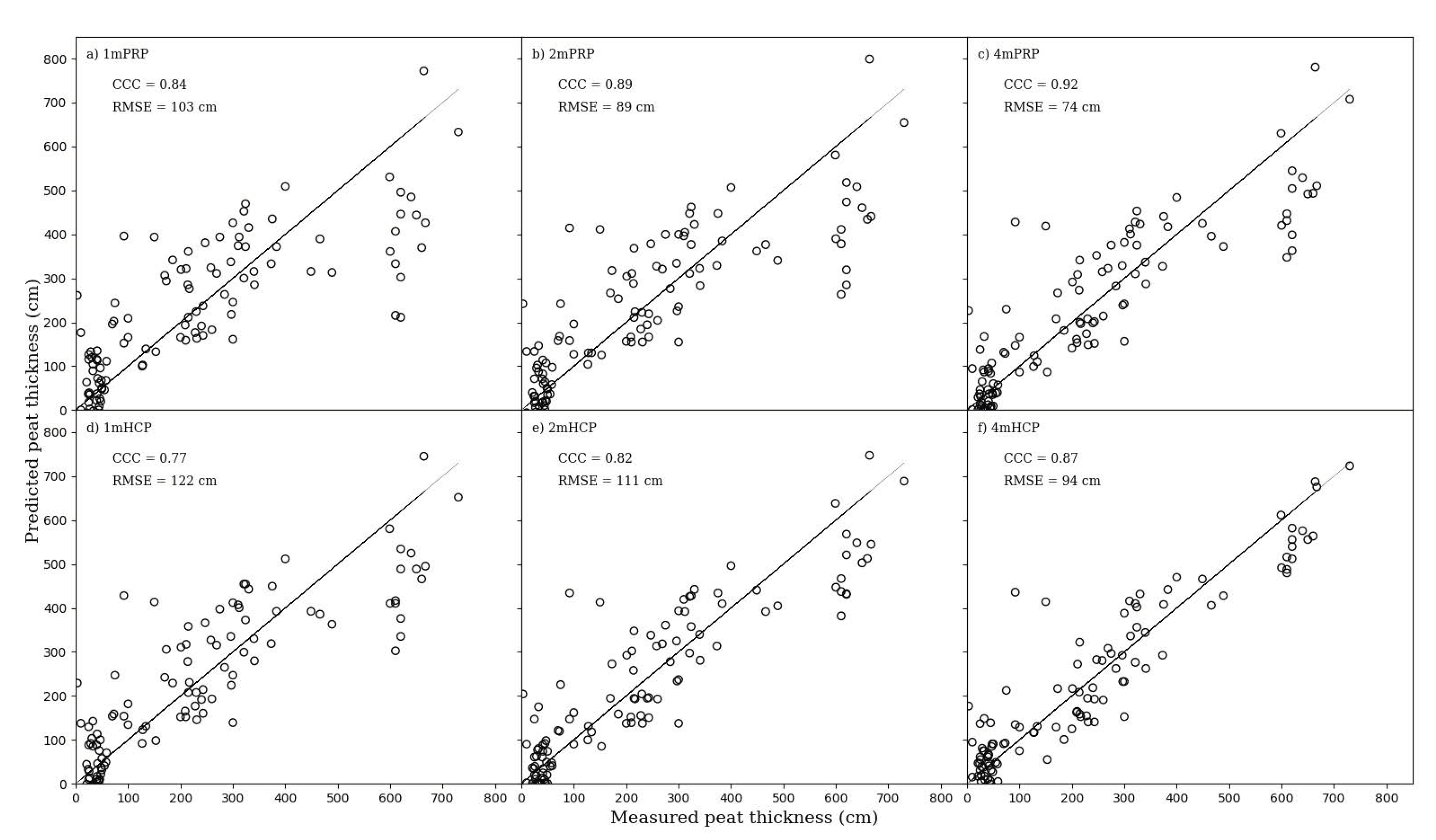
Figure 7 shows the measured peat thickness versus that predicted by the LR models for each coil configuration including the LR equations and LOOCV performance metrics. From Figure 7, it is evident that peat thickness is clearly underestimated for values larger than 500 cm, especially in the shallow measuring channels (1mPRP, 2mPRP, and 1mHCP) due to their limited DOE. The underestimation becomes less prominent with an increase in DOE, with the 4mHCP providing the most accurate predictions for the larger (i.e., >500 cm) peat thicknesses. Table 4 summarizes the LOOCV performance metrics (R2, RMSE, and CCC) for the different LR models. RMSE and CCC values ranged between 74 and 122 cm and 0.77 and 0.92, respectively. In accordance with the R2 variation previously described, the lowest RMSE and highest CCC were found for 4mHCP, while the highest RMSE and lowest CCC were recorded for 1mPRP. The RMSE variation represented about 7% of the measured peat thickness range. CCC was ranked excellent (i.e., >0.75) for all predictions using the Fleiss interpretation [46]. In accordance with Altdorff et al. [32] (2016), we suggest that these particularly good prediction results demonstrate the suitability of EMI surveys for soils with high variability.
3.5. Predicting Peat Thickness with Combinations of ECa Data and Environmental Covariates
From Table 4, we can compare the results of all models predicting peat thickness. Multiple-coil ECa MLR models yielded better predictions than single-coil ECa LR models: while R2 values were comparable or higher, RMSE and CCC were consistently lower and higher, respectively. Moreover, considering the MLR models built with different combinations of ECa data and environmental covariates, the addition of elevation data (i.e., DEM) improved the single and multiple-coil predictions. The R2 value did not increase drastically (with gains ranging from 0.02 to 0.11), which indicates that the MLR models comprising the DEM explained between 2% and 11% more variation than the LR models. While RMSE generally decreased (variation between −33 and +7 cm), CCC mostly increased (with a variation between −0.02 and +0.11). However, the addition of other terrain attributes only provided small improvements to some of the single-coil predictions and did not generate any upgrade for the multiple-coil predictions. According to Nathans et al. [47] (2012), a predictor variable displaying no or a very weak correlation to a target variable can still contribute significantly to a MLR model. Acting as a noise suppressor, the predictor variable removes irrelevant variance from other predictors within the regression [47]. In contrast to Altdorff et al. [32] (2016), the prediction accuracy was not impacted by the use of additional topography-based variables, which did not act as noise suppressors in our study. Table 4 displays the results obtained with the addition of MRVBF for illustration. Here, R2 and CCC increased by 0.01 and RMSE decreased by 1 cm for only three different combinations.
Figure 8 shows the measured peat thickness versus that predicted by the models yielding the best performances in the categories of single-coil or multiple-coil ECa models and their respective combinations with the DEM (i.e., 4mHCP, all coils, 4mHCP plus DEM and all coils plus DEM). For these selected models, R2 values ranged from 0.86 to 0.90, while RMSE values ranged from 65 to 94 cm. In particular, the predictions were more accurate for the larger (i.e., >500 cm) peat thicknesses when compared to the single-coil configurations. These results can be compared with previous DSM studies. Using elevation and slope data, Holden and Connolly [2] (2011) and Parry et al. [3] (2012) obtained lower R2 values ranging from 0.58 to 0.63 for the former and a value of 0.53 (with a RMSE of 14 cm) for the latter. Similar to Altdorff et al. [32] (2016), Parry et al. [3] (2012) suggested that the predictions were worsened in the case of shallow peat and a lesser variation in peat thickness. Several studies by Rudiyanto et al. [4,6,8] reported predictions with similar performances. Using LR or an empirical peat thickness model with elevation data, Rudiyanto et al. [4] (2015) obtained R2 values of 0.90 and 0.93 and RMSE values of 69 and 58 cm, respectively. A study by Rudiyanto et al. [6] (2016) compared four machine learning algorithms (i.e., cubist, random forest, quantile regression forest and artificial neural networks) using several environmental covariates (i.e., elevation, slope, aspect, SAGAWI and nearest distance to river). The best models yielded R2 values ranging from 0.67 to 0.92 and RMSE values ranging from 60 to 110 cm. Finally, Rudiyanto et al. [8] (2018) compared an array of machine learning algorithms (e.g., partial least squares regression, cubist, random forest, quantile regression forest, artificial neural networks and support vector machines) using many environmental covariates (i.e., DEM and derived terrain attributes, Euclidean distances to water bodies and radar and optical satellite images). The best models demonstrated better performance for calibration data (R2 from 0.95 to 0.99, and RMSE from 28 to 110 cm) than for validation data (with all models presenting similar mean values of R2 and RMSE of 0.6 and 250 cm, respectively). Notably, the predictions of these studies were carried out on larger study areas (ranging from 1000 to 100,000 ha).
3.6. Predicting Peat Thickness from Average Calculated Using a Quasi-3D Inversion Algorithm
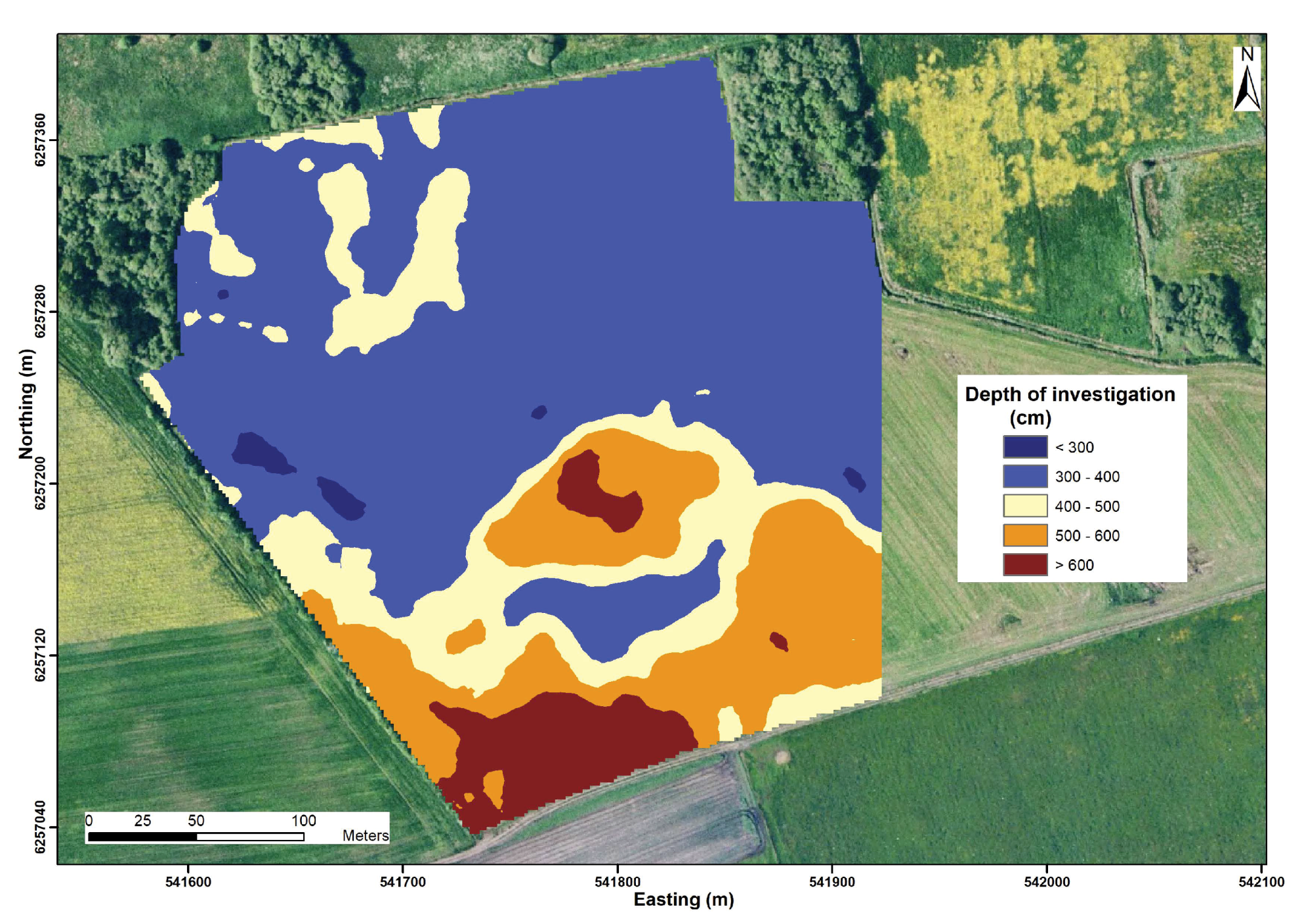
For each soil observation site, we calculated the average value from the estimates for the range corresponding to the peat thickness measured at the specific point. For instance, for the soil observation site with the maximum measured thickness of 730 cm, we calculated the average value from 15 estimates derived for each 50 cm layer corresponding to the depth interval from 0 down to 750 cm. Table 4 summarizes the LOOCV performance metrics for the LR models between peat thickness and the different average estimates. The three metrics were similar for the six different inversion models. In comparison with the predictions obtained from single-coil ECa, -based predictions were poorer for all metrics: R2 and CCC values were lower (ranging between 0.48 and 0.51, and 0.65 and 0.68, respectively) while RMSE values were higher (ranging between 141 and 145 cm). R2 values indicate that the -based models explain between 12% and 38% less variation, and CCC values were ranked as fair to good [46]. Altdorff et al. [32] (2016) reported that inversion did not provide substantial estimates of peat thickness. However, they associated these weak results to the narrow range of peat thickness in their study area, among others, which is not the case in the present investigation. While represents the true electrical conductivity estimated at different depth intervals for a specific location, the peat thickness corresponds to a sole measurement at a precise location. It is therefore difficult to predict peat thickness directly from estimates. We attempted to avoid this pitfall by calculating the average separately for each soil observation site; unfortunately, this still resulted in poor predictions in comparison with the predictions made directly from ECa. One explanation lies in the DOI. Figure 9 shows the DOI for smooth, which provided the lowest total residual of 0.88 out of all models: two-layered (1.73), three-layered (1.43), four-layered (1.20), blocky (0.91) and sharp (0.98). The smooth model was selected for illustration as it requires the least strict assumptions regarding the subsurface architecture and provides reasonable estimates in most cases. From Figure 9, areas with expected peat layers located in the northern half of the study area presented a shallow DOI (generally smaller than 400 cm, which is the average DOI value considering the whole study area). These shallow DOIs could explain the poor predictions for areas with peat layers thicker than 400 cm.
Although the inversions yielded poorer predictions, they can be advantageous to understand the conductivity distribution with depth. This is particularly important as the electrical conductivity of peat is highly dependent on the water content [10,11,12]. After inverting the data, we have derived the distribution of smooth estimates at the 110 observation points (Figure 10) to determine if there was a contrast between the peat and underlying layers. We observed that the transition is more gradual; however, overall, it can be deduced that the peat presents a conductive overburden on resistive sandy soils.
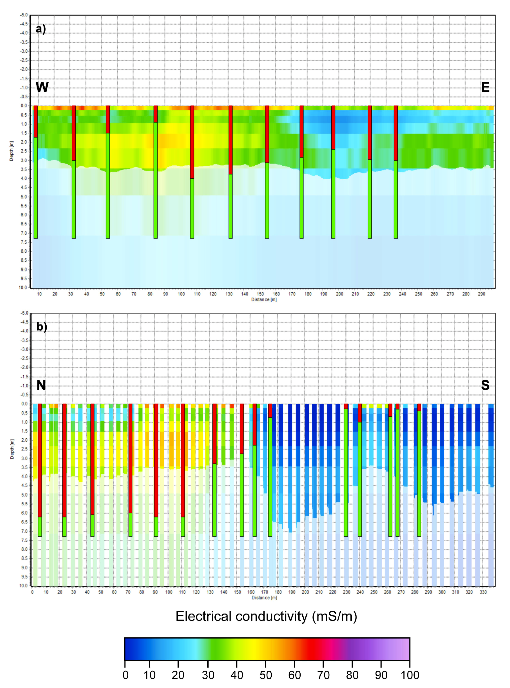
Two cross-sections (i.e., S1 and S2, represented in Figure 4) showing the calculated smooth estimates are used for further interpretation (Figure 11). S1 is approximately oriented in the west–east direction and S2 in the north-.south direction (Figure 4). S1 is located in the northern half of the study area; accordingly, the soil observation sites along this cross-section mostly present relatively large peat thicknesses (i.e., >250 cm). Along S1 (Figure 11a), the correlations between and peat thickness were not evident. For example, large peat thicknesses occur to the eastern side (i.e., 170–290 m in the profile) even though values were low (i.e., <25 mS/m) in the topsoil (i.e., 0–2 m). Likewise, the values were generally high to the western side (i.e., 0–90 m in the profile) where the observed peat thicknesses were small. Interestingly, the expected relationship (i.e., high at large peat thickness locations) was only observed at the center of the profile (i.e., within 100–160 m). These variations could result from variations in water content or cation exchange capacity within the soil, which are associated with peat properties such as bulk density, SOC content and degree of decomposition [32]. However, the expected patterns were evidently observed along S2—a cross-section along which high variability in peat thicknesses was observed (Figure 4). Along S2 (Figure 11b), the section to the northern side showed higher values where relatively large peat thicknesses (i.e., >250 cm) occur, in comparison to the southern side with shallow or no peat. In both cross-sections, it can be seen that the DOI does not reach the bottom of peat layers at the locations where the values were high, thereby limiting our capability for interpretation.
3.7. Predictive Maps for Peat Thickness
Predictive maps for peat thickness were generated using ordinary kriging within ArcMap [39]. Figure 12 displays the interpolated contour plots for peat thickness predicted by the single-coil ECa LR models. All six predictive maps show the same general pattern with a decrease of peat thickness from north to south over the study area, which is consistent with Figure 4. The main variation is in the size of the area, with a predicted peat thickness larger than 500 cm in the northern part of the study area. This area increases with the theoretical DOE of the measuring coil arrays. Figure 13 presents the predictions from the four best models selected previously (i.e., 4mHCP, all coils, 4mHCP plus DEM and all coils plus DEM). These four models show the same general patterns, with the only clear variation being the extent of the predicted areas with the largest and smallest peat thicknesses in the northern and southern parts of the study area, respectively.
3.8. Uncertainty Assessment
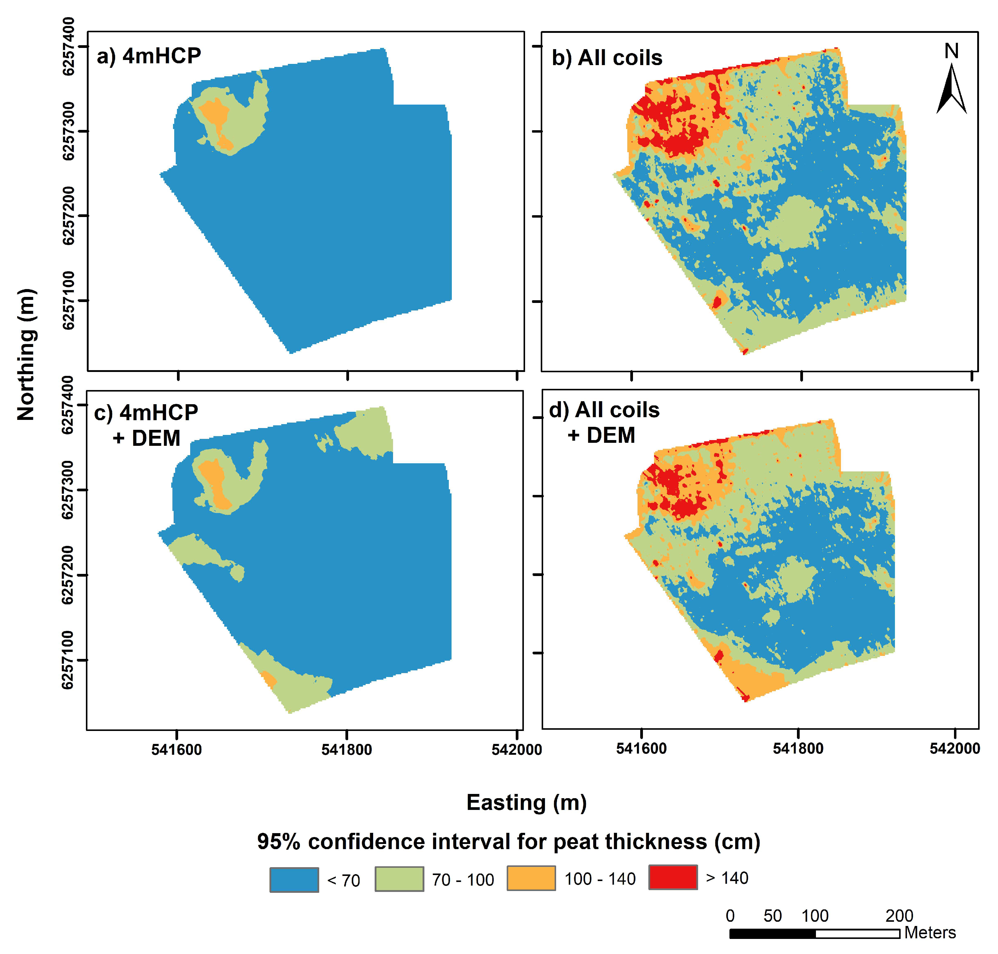
Figure 14 shows the 95% confidence interval (CI) for each selected model over the study area. The northwestern part of the study area presents both the largest predicted peat thickness values and the largest CIs in all four models. The large CIs in this particular area can be explained by (a) a relative under-sampling in comparison with the middle/southern areas (Figure 1); (b) the limitation due to the DOE for 4mHCP (i.e., 0 to 640 cm) when the largest peat thickness recorded in the area was 730 cm and (c) the fact that the DUALEM-421S could not be used to survey two small areas covered by overly dense vegetation resulting from the former plot experiment (Figure 2). The other area with large CIs in three models (i.e., 4mHCP plus DEM, all coils and all coils plus DEM) is located in the southwestern part of the study area and presents small predicted peat thickness values (Figure 13b–d). The large CIs in this specific area can be attributed to the lack of soil observations (Figure 1). Notably, the CIs for peat thickness predictions are much smaller for 4mHCP and 4mHCP plus DEM models (Figure 14a,c) than for all coils and all coils plus DEM models (Figure 14b,d). These results suggest that the single-coil predictions, using 4mHCP with or without the DEM as an additional predictor, provided the most reliable results (i.e., high accuracy and low uncertainty) in our case, which can be further used for decision-making; for example, in the case of peatland restoration.
4. Conclusions
The present case study demonstrated that data collected with a single-frequency multi-receiver electromagnetic induction (EMI) instrument enabled the non-invasive and reliable prediction of peat thickness over a 10 ha field. The results indicated that raw ECa data can already constitute valuable predictors for peat thickness (i.e., within single-coil predictions). The use of estimates calculated from quasi-3D inversion resulted in poor predictions for this case study. This outcome can be explained by the shallow depths of investigation obtained in areas with thick peat layers after the inversion of the ECa measurements. Peat thickness could also be predicted with multiple linear regression based on the combination of ECa data (i.e., multiple-coil predictions), and further with the addition of environmental covariates (i.e., elevation and different derived terrain attributes). While multiple-coil predictions and the addition of elevation data generally provided slightly higher accuracies than single-coil predictions, their corresponding uncertainty estimates calculated from 95% confidence intervals were larger. Therefore, we suggest that for our case study, the single-coil predictions—in particular using 4mHCP with or without elevation as an additional predictor—provided the most reliable results (i.e., high accuracy and low uncertainty) for use in decision-making; for example, in the case of peatland restoration. Notably, the significant results obtained in this study can be explained by the high variability in peat thickness of the selected field area. Finally, this study demonstrates the considerable potential of EMI data for use in peat thickness mapping.
A future development of the present study will aim at the intensive investigation of the spatial variability of different key peat soil properties, such as soil organic carbon content, bulk density and soil organic carbon stock. This subsequent study would greatly benefit from inversion modeling and the use of an EMI instrument which can reach a larger DOI over the whole field, yielding more detailed information on the peat and underlying layers. To achieve this, a comprehensive soil sampling procedure guided by a more appropriate soil sampling design (for example, from a conditioned Latin hypercube sampling approach; the procedure in [48] can be adopted to measure different soil properties at consistent depth intervals). Furthermore, this study can greatly benefit from the use of a combination of complementary techniques such as visible near-infrared (vis–NIR) spectroscopy for a more accurate representation of peat and the underlying layers. Fusing EMI and vis–NIR data will allow the SOC content to be mapped at different depths and enable the further assessment of the SOC stocks over the study area.
Author Contributions
Conceptualization: A.B. and T.K.; data curation: A.B. and T.K.; visualization: A.B.; supervision and funding: M.H.G. and B.V.I.; writing—original draft preparation: A.B. and T.K.; writing—review and editing: M.H.G. and B.V.I.; methodology, software, and validation: A.B. and T.K. All authors have read and agreed to the published version of the manuscript.
Funding
This research received no external funding.
Acknowledgments
The authors would like to thank Henrik No rgaard for assisting with the collection of DUALEM data and Jesper Bjergsted Pedersen for help with the Aarhus Workbench software.
Conflicts of Interest
The authors declare no conflict of interest.
References
- European Parliament. Inclusion of greenhouse gas emissions and removals from land use, land use change and forestry into the 2030 climate and energy framework. In P8-TA-PROV(2018)0096; Parliament, E., Ed.; European Parliament: Strasbourg, France, 2018. [Google Scholar]
- Holden, N.M.; Connolly, J. Estimating the carbon stock of a blanket peat region using a peat depth inference model. Catena 2011, 86, 75–85. [Google Scholar] [CrossRef]
- Parry, L.E.; Charman, D.J.; Noades, J.P. A method for modelling peat depth in blanket peatlands. Soil Use Manag. 2012, 28, 614–624. [Google Scholar] [CrossRef]
- Rudiyanto; Setiawan, B.I.; Arief, C.; Saptomo, S.K.; Gunawan, A.; Kuswarman; Sungkono; Indriyanto, H. Estimating Distribution of Carbon Stock in Tropical Peatland Using a Combination of an Empirical Peat Depth Model and GIS. Procedia Environ. Sci. 2015, 24, 152–157. [Google Scholar] [CrossRef] [Green Version]
- Hooijer, A.; Vernimmen, R. Peatland Maps for Indonesia. Including Accuracy Assessment and Recommendations for Improvement, Elevation Mapping and Evaluation of Future Flood Risk. Quick Assessment and Nationwide Screening (QANS) of Peat and Lowland Resources and Action Planning for the Implementation of a National Lowland Strategy-PVW3A10002; 2013; Available online: https://www.deltares.nl/app/uploads/2015/03/QANS-Peat-mapping-report-final-with-cover.pdf (accessed on 20 July 2020).
- Rudiyanto; Minasny, B.; Setiawan, B.I.; Arif, C.; Saptomo, S.K.; Chadirin, Y. Digital mapping for cost-effective and accurate prediction of the depth and carbon stocks in Indonesian peatlands. Geoderma 2016, 272, 20–31. [Google Scholar] [CrossRef]
- Aitkenhead, M.J. Mapping peat in Scotland with remote sensing and site characteristics. Eur. J. Soil Sci. 2017, 68, 28–38. [Google Scholar] [CrossRef] [Green Version]
- Rudiyanto; Minasny, B.; Setiawan, B.I.; Saptomo, S.K.; McBratney, A.B. Open digital mapping as a cost-effective method for mapping peat thickness and assessing the carbon stock of tropical peatlands. Geoderma 2018, 313, 25–40. [Google Scholar] [CrossRef]
- Young, D.M.; Parry, L.E.; Lee, D.; Ray, S. Spatial models with covariates improve estimates of peat depth in blanket peatlands. PLoS ONE 2018, 13, 1–19. [Google Scholar] [CrossRef] [PubMed]
- Asadi, A.; Huat, B.B. Electrical resistivity of tropical peat. Electron. J. Geotech. Eng. 2009, 14, 1–9. [Google Scholar]
- Ponziani, M.; Slob, E.C.; Ngan-Tillard, D.J.M.; Vanhala, H. Influence of water content on the electrical conductivity of peat. Int. Water Technol. J. 2011, 1, 14–21. [Google Scholar]
- Walter, J.; Lück, E.; Bauriegel, A.; Richter, C.; Zeitz, J. Multi-scale analysis of electrical conductivity of peatlands for the assessment of peat properties. Eur. J. Soil Sci. 2015, 66, 639–650. [Google Scholar] [CrossRef]
- Minasny, B.; Berglund, Ö.; Connolly, J.; Hedley, C.; de Vries, F.; Gimona, A.; Kempen, B.; Kidd, D.; Lilja, H.; Malone, B.; et al. Digital mapping of peatlands—A critical review. Earth-Sci. Rev. 2019, 196, 102870. [Google Scholar] [CrossRef]
- Silvestri, S.; Christensen, C.W.; Lysdahl, A.O.; Anschütz, H.; Pfaffhuber, A.A.; Viezzoli, A. Peatland Volume Mapping Over Resistive Substrates With Airborne Electromagnetic Technology. Geophys. Res. Lett. 2019, 46, 6459–6468. [Google Scholar] [CrossRef] [Green Version]
- Silvestri, S.; Knight, R.; Viezzoli, A.; Richardson, C.J.; Anshari, G.Z.; Dewar, N.; Flanagan, N.; Comas, X. Quantification of Peat Thickness and Stored Carbon at the Landscape Scale in Tropical Peatlands: A Comparison of Airborne Geophysics and an Empirical Topographic Method. J. Geophys. Res. Earth Surf. 2019, 124, 3107–3123. [Google Scholar] [CrossRef] [Green Version]
- Siemon, B.; Ibs-von Seht, M.; Frank, S. Airborne electromagnetic and radiometric peat thickness mapping of a bog in Northwest Germany (Ahlen-Falkenberger Moor). Remote Sens. 2020, 12, 203. [Google Scholar] [CrossRef] [Green Version]
- Siemon, B.; von Seht, M.I.; Steuer, A.; Deus, N.; Wiederhold, H. Airborne electromagnetic, magnetic, and radiometric surveys at the German North Sea coast applied to groundwater and soil investigations. Remote Sens. 2020, 12, 1629. [Google Scholar] [CrossRef]
- Theimer, B. Principles of Bog Characterization Using Ground Penetrating Radar. Master’s Thesis, University of Waterloo, Waterloo, ON, USA, 1990. [Google Scholar]
- Theimer, B.D.; Nobes, D.C.; Warner, B.G. A study of the geoelectrical properties of peatlands and their influence on ground-penetrating radar surveying. Geophys. Prospect. 1994, 42, 179–209. [Google Scholar] [CrossRef]
- Holden, J.; Burt, T.P.; Vilas, M. Application of ground-penetrating radar to the identification of subsurface piping in blanket peat. Earth Surf. Process. Landf. 2002, 27, 235–249. [Google Scholar] [CrossRef]
- Slater, L.D.; Reeve, A. Investigating peatland stratigraphy and hydrogeology using integrated electrical geophysics. Geophysics 2002, 67, 365–378. [Google Scholar] [CrossRef] [Green Version]
- Rosa, E.; Larocque, M.; Pellerin, S.; Gagné, S.; Fournier, B. Determining the number of manual measurements required to improve peat thickness estimations by ground penetrating radar. Earth Surf. Process. Landf. 2009, 34, 377–383. [Google Scholar] [CrossRef]
- Kettridge, N.; Comas, X.; Baird, A.; Slater, L.; Strack, M.; Thompson, D.; Jol, H.; Binley, A. Ecohydrologically important subsurface structures in peatlands revealed by ground-penetrating radar and complex conductivity surveys. J. Geophys. Res. Biogeosci. 2008, 113, 1–15. [Google Scholar] [CrossRef] [Green Version]
- Sass, O.; Friedmann, A.; Haselwanter, G.; Wetzel, K.F. Investigating thickness and internal structure of alpine mires using conventional and geophysical techniques. Catena 2010, 80, 195–203. [Google Scholar] [CrossRef]
- Viezzoli, A.; Christiansen, A.V.; Auken, E.; Sørensen, K. Quasi-3D modeling of airborne TEM data by spatially constrained inversion. Geophysics 2008, 73, F105–F113. [Google Scholar] [CrossRef]
- Auken, E.; Christiansen, A.V.; Kirkegaard, C.; Fiandaca, G.; Schamper, C.; Behroozmand, A.A.; Binley, A.; Nielsen, E.; Effersø, F.; Christensen, N.B.; et al. An overview of a highly versatile forward and stable inverse algorithm for airborne, ground-based and borehole electromagnetic and electric data. Explor. Geophys. 2015, 46, 223–235. [Google Scholar] [CrossRef] [Green Version]
- Davies, G.; Huang, J.; Monteiro Santos, F.A.; Triantafilis, J. Modeling coastal salinity in Quasi 2D and 3D using a DUALEM-421 and inversion software. Groundwater 2015, 53, 424–431. [Google Scholar] [CrossRef]
- Zare, E.; Beucher, A.; Huang, J.; Boman, A.; Mattbäck, S.; Greve, M.H.; Triantafilis, J. Three-dimensional imaging of active acid sulfate soil using a DUALEM-21S and EM inversion software. J. Environ. Manag. 2018, 212, 99–107. [Google Scholar] [CrossRef]
- Koganti, T.; Narjary, B.; Zare, E.; Pathan, A.L.; Huang, J.; Triantafilis, J. Quantitative mapping of soil salinity using the DUALEM-21S instrument and EM inversion software. Land Degrad. Dev. 2018, 29, 1768–1781. [Google Scholar] [CrossRef]
- Comas, X.; Slater, L.; Reeve, A.S. Pool patterning in a northern peatland: Geophysical evidence for the role of postglacial landforms. J. Hydrol. 2011, 399, 173–184. [Google Scholar] [CrossRef]
- Koszinski, S.; Miller, B.A.; Hierold, W.; Haelbich, H.; Sommer, M. Spatial Modeling of organic carbon in degraded Peatland soils of northeast Germany. Soil Sci. Soc. Am. J. 2015, 79, 1496–1508. [Google Scholar] [CrossRef]
- Altdorff, D.; Bechtold, M.; van der Kruk, J.; Vereecken, H.; Huisman, J.A. Mapping peat layer properties with multi-coil offset electromagnetic induction and laser scanning elevation data. Geoderma 2016, 261, 178–189. [Google Scholar] [CrossRef]
- Boaga, J.; Viezzoli, A.; Cassiani, G.; Deidda, G.P.; Tosi, L.; Silvestri, S. Resolving the thickness of peat deposits with contact-less electromagnetic methods: A case study in the Venice coastland. Sci. Total Environ. 2020, 737, 139361. [Google Scholar] [CrossRef]
- Kandel, T.P.; Elsgaard, L.; Lærke, P.E. Annual balances and extended seasonal modelling of carbon fluxes from a temperate fen cropped to festulolium and tall fescue under two-cut and three-cut harvesting regimes. GCB Bioenergy 2017, 9, 1690–1706. [Google Scholar] [CrossRef]
- Madsen, H.B.; Nørr, A.H.; Holst, K.A. The Danish Soil Classification. Atlas Over Denmark I Vol. 3; The Royal Danish Geographical Society: Copenhagen, Denmark, 1992. [Google Scholar]
- Knadel, M.; Thomsen, A.; Greve, M.H. Multisensor on-the-go mapping of soil organic carbon content. Soil Sci. Soc. Am. J. 2011, 75, 1799–1806. [Google Scholar] [CrossRef]
- Wang, P.R. Teknisk Rapport 12-23. Referenceværdier: Måneds- og årskort 2001–2010, Danmark for Temperatur, Relativ Luftfugtighed, Vindhastighed, Globalstråling og Nedbør; 2013; pp. 1–40. Available online: https://www.dmi.dk/fileadmin/Rapporter/TR/tr12-23.pdf (accessed on 20 July 2020).
- Agency for Data Supply and Efficiency, GeoDanmark. 2019. Available online: https://sdfe.dk/hent-data/fotos-og-509geodanmark-data/ (accessed on 20 July 2020).
- ESRI. ArcGIS Desktop: Release 10.7.1; Environmental Systems Research Institute: Redlands, CA, USA, 2019. [Google Scholar]
- Everett, M. Electromagnetic induction. Near-Surface Applied Geophysics; Cambridge University Press: New York, NY, USA, 2013; pp. 200–238. [Google Scholar]
- McNeill, J.D. Electromagnetic Terrain Conductivity Measurement at Low Induction Numbers: Technical Note TN-6; Geonic Ltd.: Mississauga, ON, Canada, 1980. [Google Scholar]
- Dualem, Inc. DUALEM-21S User’s Manual; Dualem Inc.: Milton, ON, Canada, 2008. [Google Scholar]
- Auken, E.; Viezzoli, A.; Christensen, A. A single software for processing, inversion, and presentation of AEM data of different systems: The Aarhus Workbench. ASEG Ext. Abstr. 2009, 2009, 1. [Google Scholar] [CrossRef]
- Sharp Model Inversion Setup for Inversion of Geophysical Data—Guidelines and Examples. Hydrogeophysics Group, Department of Geoscience, Aarhus University, Denmark. 2018. Available online: http://www.hgg.geo.au.dk/rapporter/Sharp_report.pdf (accessed on 20 July 2020).
- Christiansen, A.V.; Pedersen, J.B.; Auken, E.; Søe, N.E.; Holst, M.K.; Kristiansen, S.M. Improved geoarchaeological mapping with electromagnetic induction instruments from dedicated processing and inversion. Remote Sens. 2016, 8, 1022. [Google Scholar] [CrossRef] [Green Version]
- Fleiss, J. Statistical Methods for Rates and Proportions, 1st ed.; John Wiley & Sons, Inc.: Hoboken, NJ, USA, 1981. [Google Scholar]
- Nathans, L.L.; Oswald, F.L.; Nimon, K. Interpreting multiple linear regression: A guidebook of variable importance. Pract. Assess. Res. Eval. 2012, 17, 1–19. [Google Scholar]
- Minasny, B.; McBratney, A.B. A conditioned Latin hypercube method for sampling in the presence of ancillary information. Comput. Geosci. 2006, 32, 1378–1388. [Google Scholar] [CrossRef]
Figure 1.
Location of soil observations collected during two sampling survey campaigns within the study area (orthophoto from the spring 2006 as background [38]).
Figure 1.
Location of soil observations collected during two sampling survey campaigns within the study area (orthophoto from the spring 2006 as background [38]).
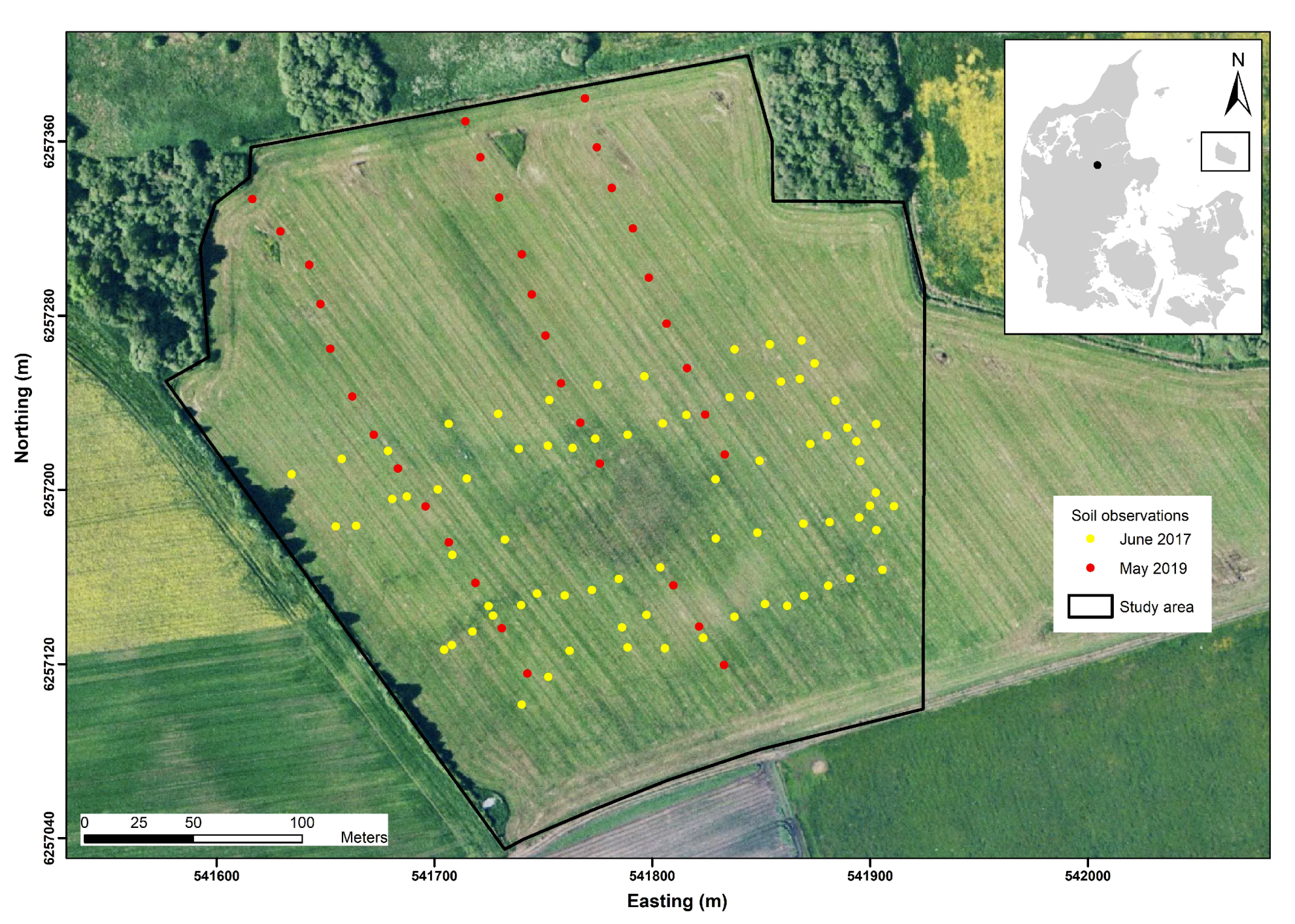
Figure 2.
Location of the DUALEM-421S survey transects within the study area.

Figure 3.
Examples of environmental covariates tested for the prediction of peat thickness: (a) Digital Elevation Model (DEM), (b) slope gradient, (c) Multi-Resolution Index of Valley Bottom Flatness (MRVBF), and (d) System of Automated Geoscientific Analyses Wetness Index (SAGAWI).
Figure 3.
Examples of environmental covariates tested for the prediction of peat thickness: (a) Digital Elevation Model (DEM), (b) slope gradient, (c) Multi-Resolution Index of Valley Bottom Flatness (MRVBF), and (d) System of Automated Geoscientific Analyses Wetness Index (SAGAWI).

Figure 4.
Peat thickness (cm) measured at soil observation points and locations of cross-sections S1 and S2.
Figure 4.
Peat thickness (cm) measured at soil observation points and locations of cross-sections S1 and S2.
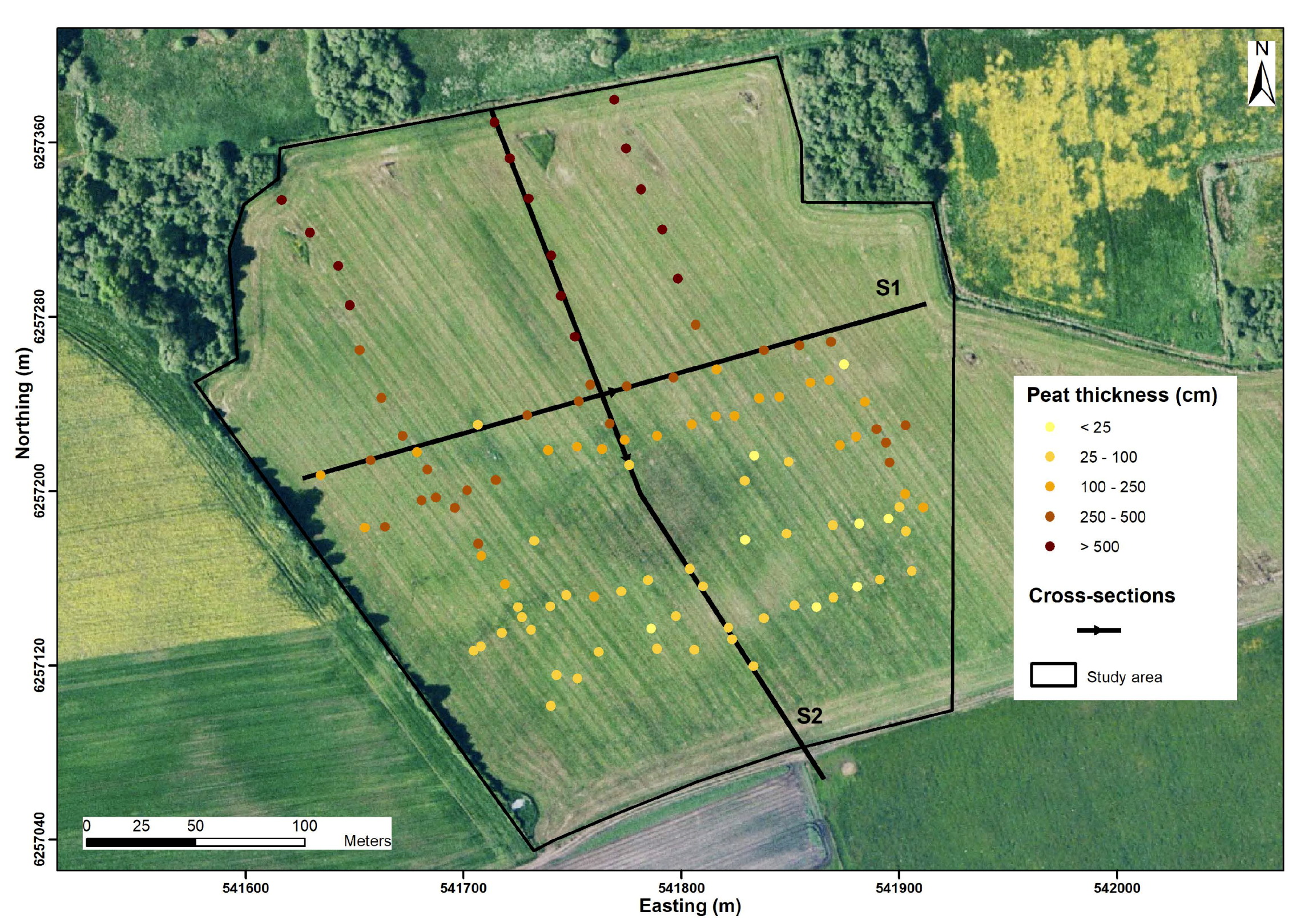
Figure 5.
Contour plots of the interpolated apparent electrical conductivity (ECa—mS/m) collected using the six different coils configurations of a DUALEM-421S instrument: (a) 1mPRP, (b) 1mHCP, (c) 2mPRP, (d) 2mHCP, (e) 4mPRP and (f) 4mHCP.
Figure 5.
Contour plots of the interpolated apparent electrical conductivity (ECa—mS/m) collected using the six different coils configurations of a DUALEM-421S instrument: (a) 1mPRP, (b) 1mHCP, (c) 2mPRP, (d) 2mHCP, (e) 4mPRP and (f) 4mHCP.
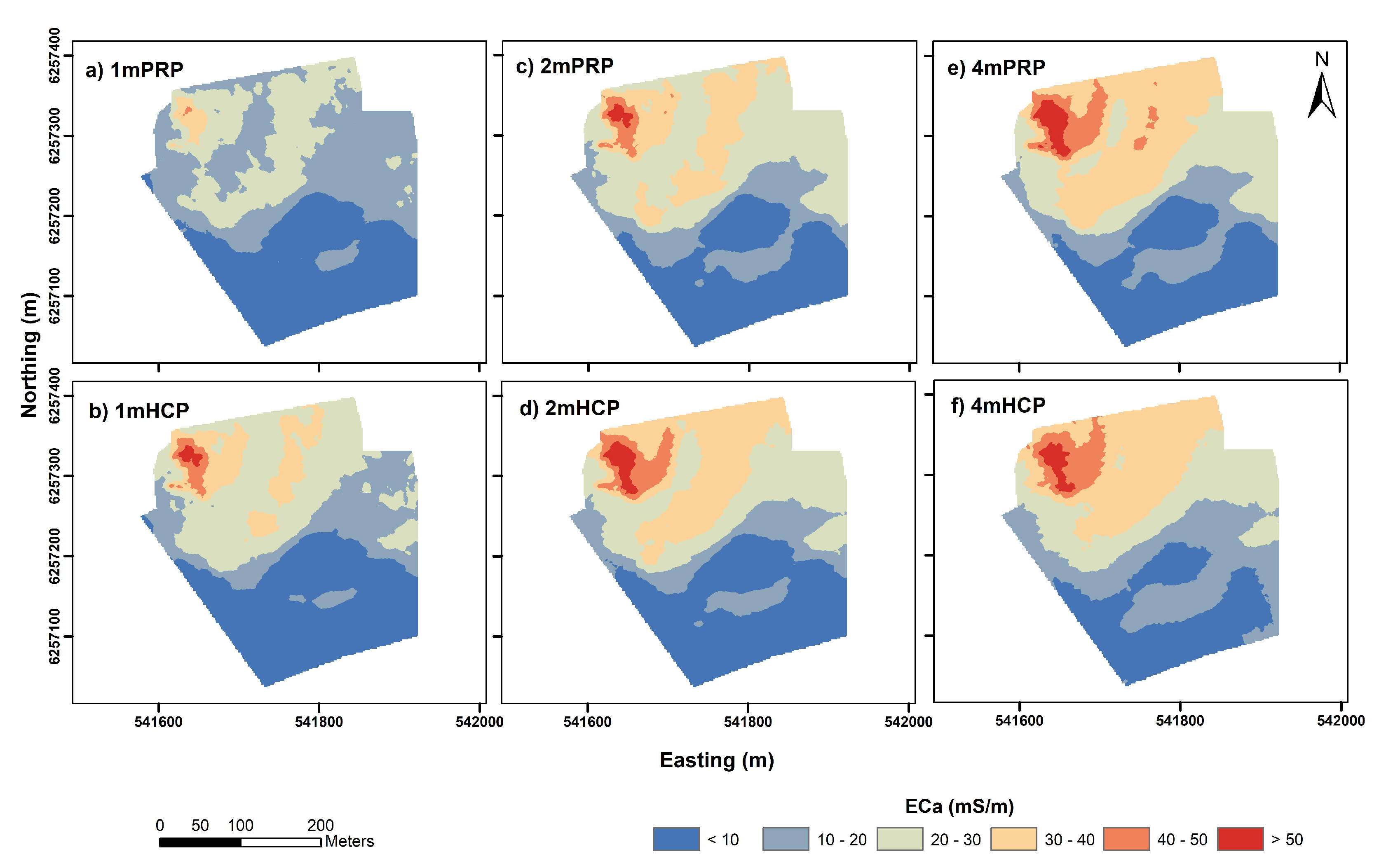
Figure 6.
Measured peat thickness (cm) vs. measured apparent electrical conductivity (ECa—mS/m) collected using the six different coil configurations of a DUALEM-421S instrument: (a) 1mPRP, (b) 2mPRP, (c) 4mPRP, (d) 1mHCP, (e) 2mHCP and (f) 4mHCP (fitted regression line represented on each plot).
Figure 6.
Measured peat thickness (cm) vs. measured apparent electrical conductivity (ECa—mS/m) collected using the six different coil configurations of a DUALEM-421S instrument: (a) 1mPRP, (b) 2mPRP, (c) 4mPRP, (d) 1mHCP, (e) 2mHCP and (f) 4mHCP (fitted regression line represented on each plot).
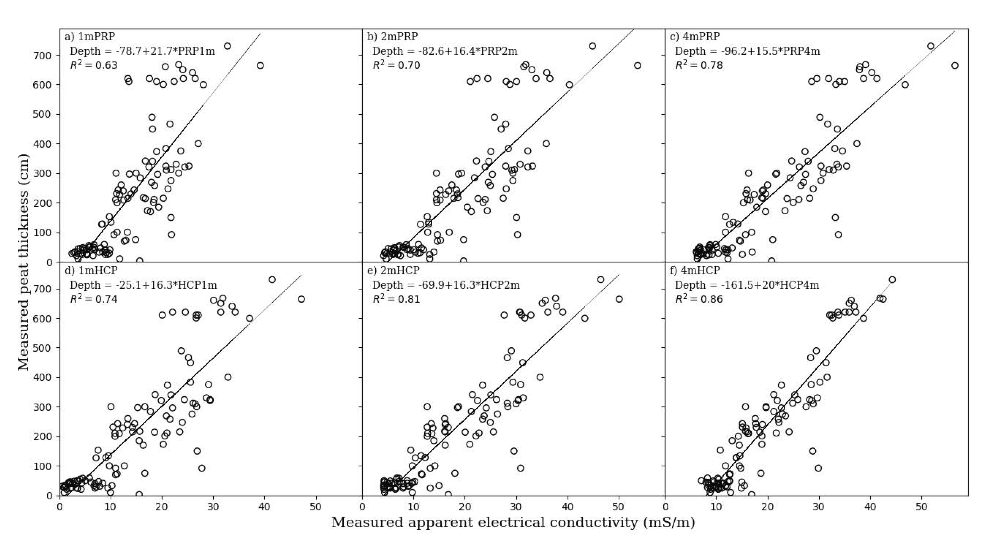
Figure 7.
Measured vs. predicted peat thickness (cm) using leave-one-out cross validation (LOOCV) for ECa collected from the six different coil configurations of a DUALEM-421S instrument: (a) 1mPRP, (b) 2mPRP, (c) 4mPRP, (d) 1mHCP, (e) 2mHCP and (f) 4mHCP (1:1 identity line represented on each plot).

Figure 8.
Measured vs. predicted peat thickness (cm) using (a) 4mHCP, (b) the combination of all six coils, (c) the combination of 4mHCP and DEM and (d) the combination of all six coils and DEM (1:1 identity line represented on each plot).
Figure 8.
Measured vs. predicted peat thickness (cm) using (a) 4mHCP, (b) the combination of all six coils, (c) the combination of 4mHCP and DEM and (d) the combination of all six coils and DEM (1:1 identity line represented on each plot).

Figure 9.
Depth of investigation (DOI) for the calculated true electrical conductivity (smooth) estimates over the study area.
Figure 9.
Depth of investigation (DOI) for the calculated true electrical conductivity (smooth) estimates over the study area.

Figure 10.
Distribution of the calculated average true electrical conductivity (smooth) estimates over the study area for peat and the underlying layers.
Figure 10.
Distribution of the calculated average true electrical conductivity (smooth) estimates over the study area for peat and the underlying layers.
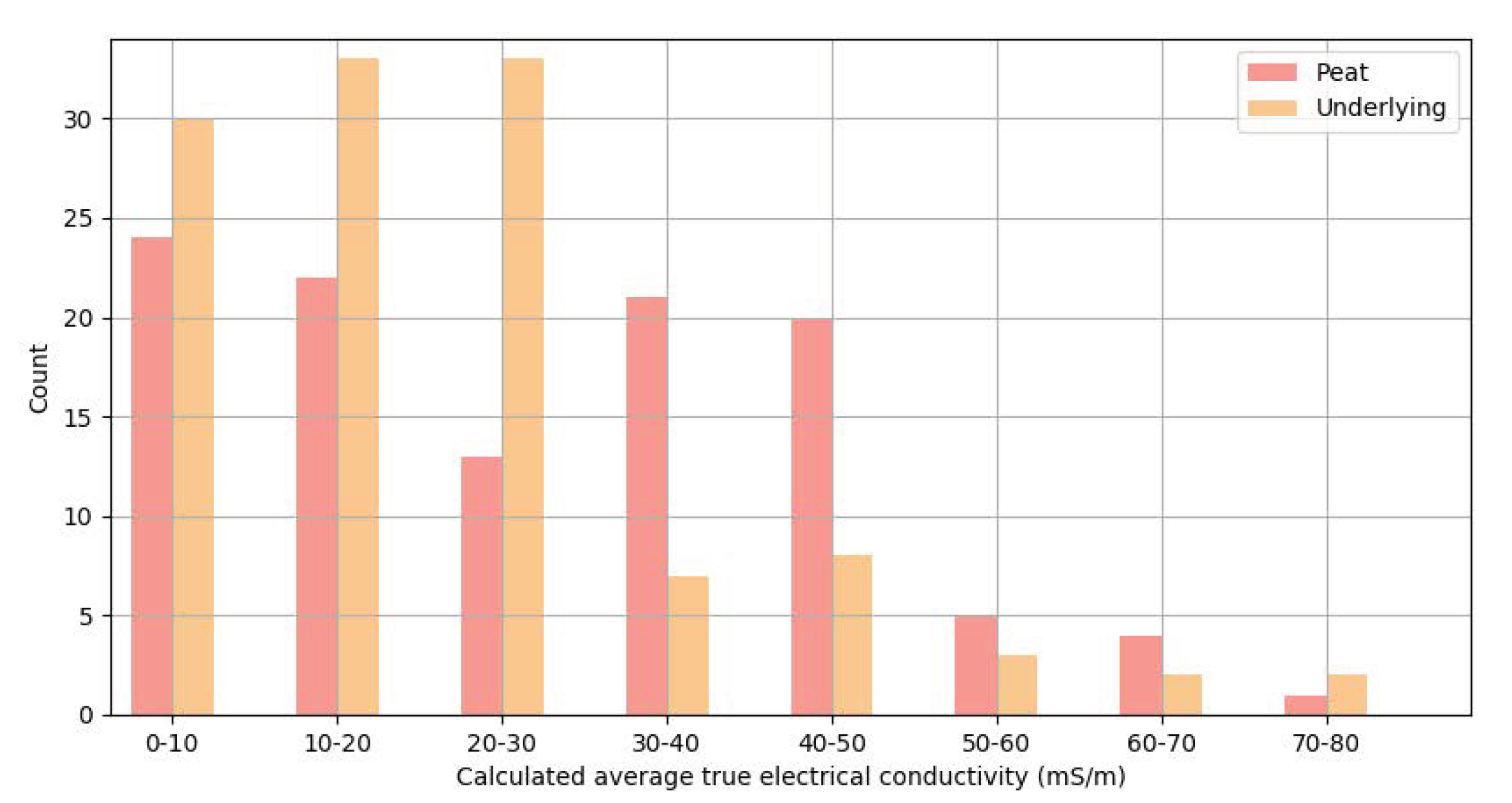
Figure 11.
Cross-sections S1 (a) and S2 (b) showing the calculated smooth estimates (for each soil observation site, peat layers are represented in red and underlying layers in green).
Figure 11.
Cross-sections S1 (a) and S2 (b) showing the calculated smooth estimates (for each soil observation site, peat layers are represented in red and underlying layers in green).

Figure 12.
Contour plots of the interpolated peat thickness (cm) predicted from the apparent electrical conductivity (ECa—mS/m) collected using the six different coil configurations of a DUALEM-421S instrument: (a) 1mPRP, (b) 1mHCP, (c) 2mPRP, (d) 2mHCP, (e) 4mPRP and (f) 4mHCP.
Figure 12.
Contour plots of the interpolated peat thickness (cm) predicted from the apparent electrical conductivity (ECa—mS/m) collected using the six different coil configurations of a DUALEM-421S instrument: (a) 1mPRP, (b) 1mHCP, (c) 2mPRP, (d) 2mHCP, (e) 4mPRP and (f) 4mHCP.
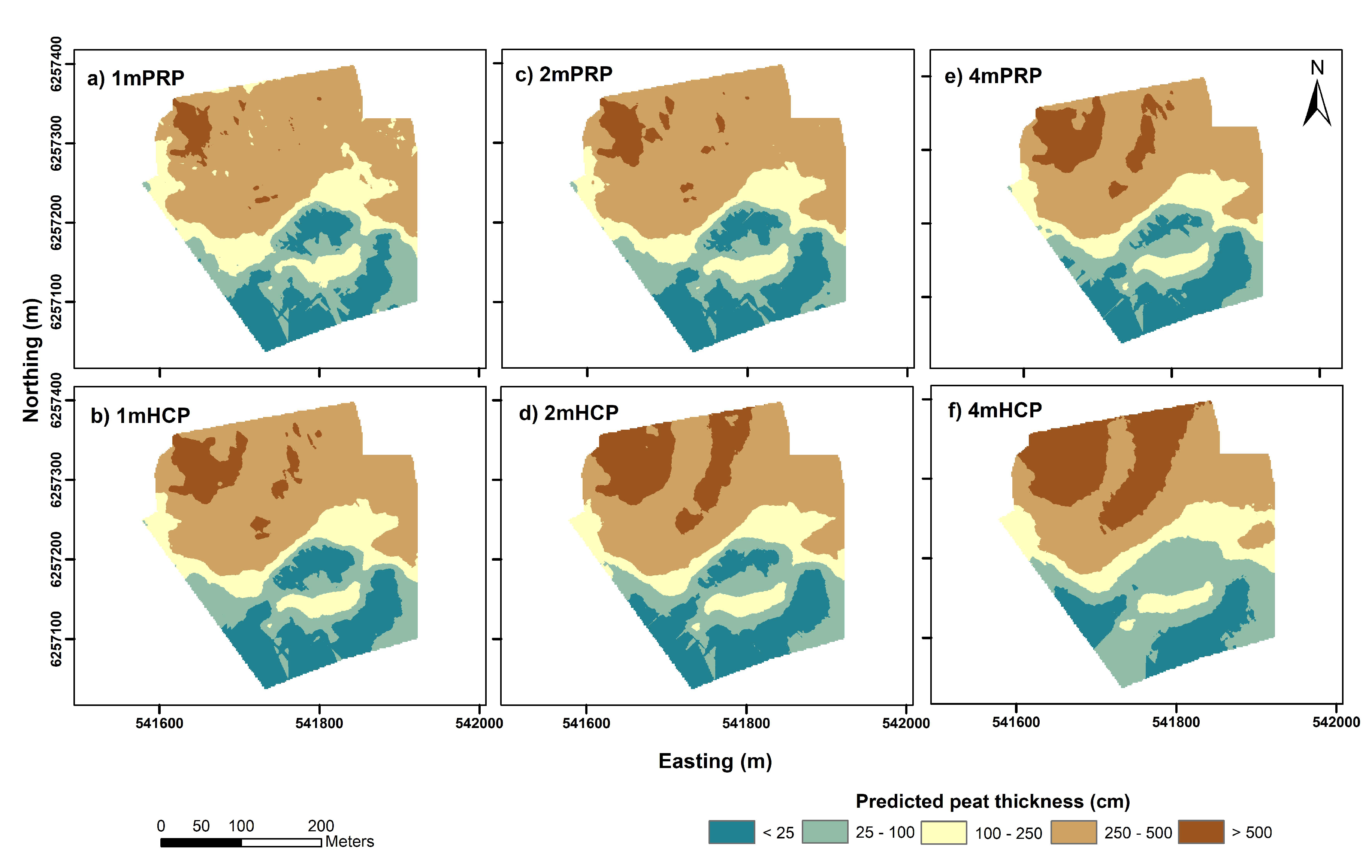
Figure 13.
Contour plots of the interpolated peat thickness (cm) predicted from (a) 4mHCP, (b) the combination of all six coils, (c) the combination of 4mHCP and the DEM and (d) the combination of all six coils and the DEM.
Figure 13.
Contour plots of the interpolated peat thickness (cm) predicted from (a) 4mHCP, (b) the combination of all six coils, (c) the combination of 4mHCP and the DEM and (d) the combination of all six coils and the DEM.
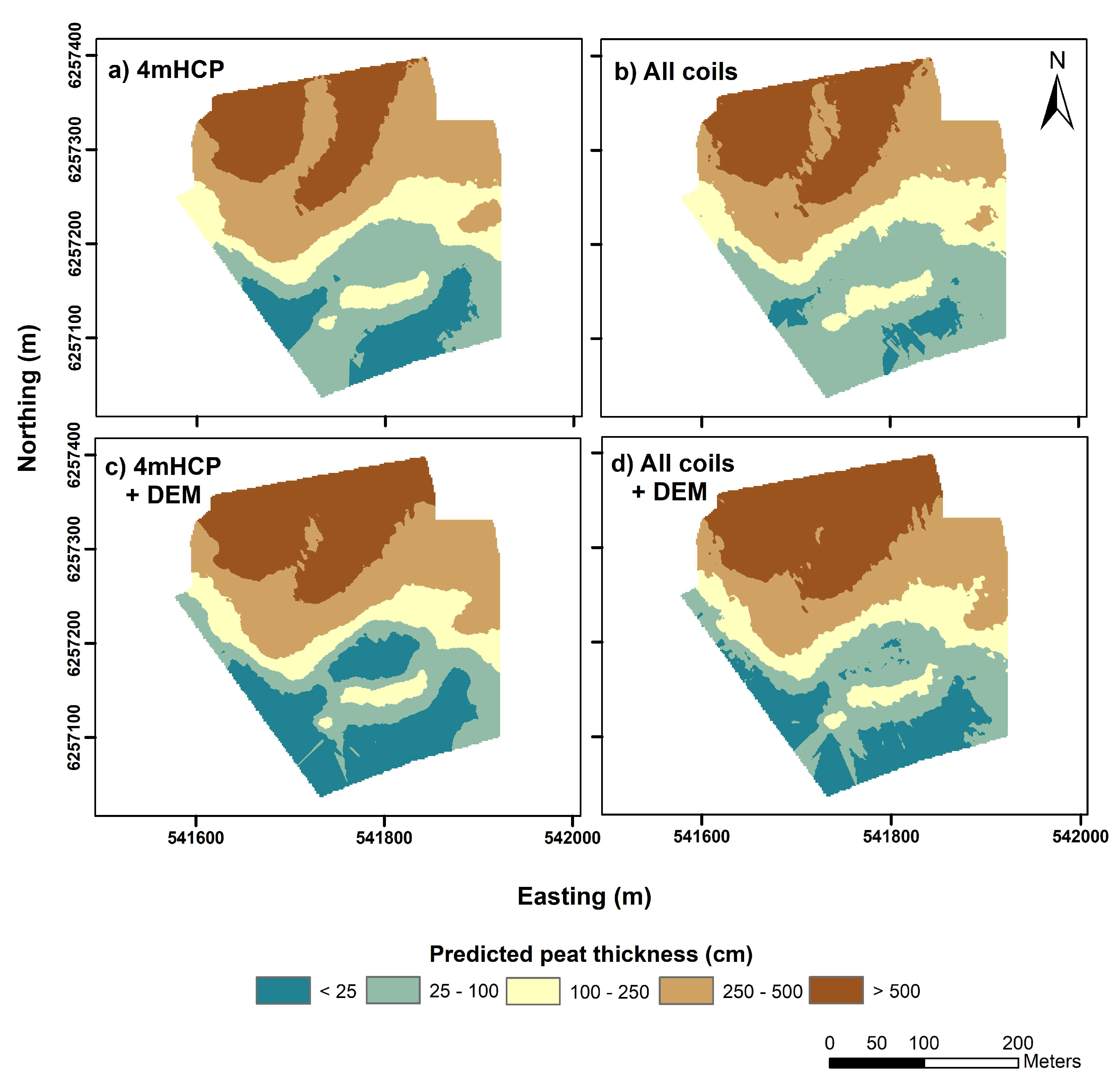
Figure 14.
Plots of 95% confidence intervals for the peat thickness (cm) predicted from (a) 4mHCP, (b) the combination of all six coils, (c) the combination of 4mHCP and the DEM and (d) the combination of all six coils and the DEM.
Figure 14.
Plots of 95% confidence intervals for the peat thickness (cm) predicted from (a) 4mHCP, (b) the combination of all six coils, (c) the combination of 4mHCP and the DEM and (d) the combination of all six coils and the DEM.

Table 1.
Summary statistics for the apparent electrical conductivity (ECa—mS/m) measured by a DUALEM-421S for the whole survey area and at the soil observation sites.
Table 1.
Summary statistics for the apparent electrical conductivity (ECa—mS/m) measured by a DUALEM-421S for the whole survey area and at the soil observation sites.
| ECa (mS/m) | |||||||
|---|---|---|---|---|---|---|---|
| Data Source | n | Min. | Mean | Median | Max. | Skewness | CV (%) |
| Survey data | |||||||
| 1mPRP | 48,150 | 3.7 | 17.1 | 17.5 | 43.6 | 0.17 | 37.4 |
| 1mHCP | 48,150 | 1.6 | 20.9 | 21.8 | 56.4 | 0.09 | 47.8 |
| 2mPRP | 48,150 | 5.1 | 23.7 | 24.5 | 58 | 0.07 | 39 |
| 2mHCP | 48,150 | 4.3 | 24.7 | 25.5 | 62.6 | 0.14 | 45.9 |
| 4mPRP | 48,150 | 6.2 | 27.1 | 28.1 | 65.9 | 0.12 | 41.4 |
| 4mHCP | 48,150 | 8.1 | 25.6 | 25.1 | 60.8 | 0.29 | 41.6 |
| Soil observation sites | |||||||
| 1mPRP | 110 | 2.5 | 14.1 | 13.4 | 39.2 | 0.47 | 52.4 |
| 1mHCP | 110 | 0.6 | 15.5 | 14.3 | 47.2 | 0.46 | 68.7 |
| 2mPRP | 110 | 4.2 | 18.9 | 17.9 | 53.7 | 0.54 | 54.5 |
| 2mHCP | 110 | 4.2 | 18.2 | 16.1 | 50.1 | 0.59 | 61.2 |
| 4mPRP | 110 | 6.1 | 20.8 | 19 | 56.5 | 0.60 | 55.3 |
| 4mHCP | 110 | 7.1 | 19.4 | 16.2 | 44.3 | 0.76 | 48.5 |
n: number of measurements/observations; Min.: minimum; Max.: maximum; CV: coefficient of variation; PRP: perpendicular coplanar coil array; HCP: horizontal coplanar coil array.
Table 2.
Summary statistics for peat thickness at the soil observation sites.
| Soil Observation Sites | n | Min. | Mean | Median | Max. | Skewness | CV (%) |
|---|---|---|---|---|---|---|---|
| Peat thickness (cm) | 110 | 3 | 230 | 210 | 730 | 0.91 | 89.7 |
n: number of measurements/observations; Min.: minimum; Max.: maximum; CV: coefficient of variation.
Table 3.
Pearson’s r correlation coefficient between the target variable (i.e., peat thickness) and the ECa, and topography-based predictor variables.
Table 3.
Pearson’s r correlation coefficient between the target variable (i.e., peat thickness) and the ECa, and topography-based predictor variables.
| 1mPRP | 1mHCP | 2mPRP | 2mHCP | 4mPRP | 4mHCP | ||
| 0.80 | 0.86 | 0.84 | 0.90 | 0.88 | 0.93 | ||
| 2-layered | 3-layered | 4-layered | blocky | sharp | smooth | ||
| 0.71 | 0.72 | 0.71 | 0.70 | 0.71 | 0.71 | ||
| DEM | slope | MRVBF | SAGAWI | plan curv | prof curv | cos aps | sin asp |
| −0.69 | −0.19 | 0.41 | 0.31 | −0.15 | −0.04 | 0.16 | −0.04 |
DEM: Digital Elevation Model; MRVBF: Multi-Resolution Index of Valley Bottom Flatness; SAGAWI: System of Automated Geoscientific Analyses Wetness Index; prof curv: profile curvature; plan curv: plan curvature; cos asp and sin asp: cosine and sine of aspect.
Table 4.
LOOCV performance metrics for models predicting peat thickness from single-coil ECa data (LR), different combinations of ECa data (i.e., multiple-coil predictions) and environmental covariates (MLR), and from the average calculated using different inversion models (LR).
Table 4.
LOOCV performance metrics for models predicting peat thickness from single-coil ECa data (LR), different combinations of ECa data (i.e., multiple-coil predictions) and environmental covariates (MLR), and from the average calculated using different inversion models (LR).
| R2 | RMSE (cm) | CCC | |
|---|---|---|---|
| Single-coil ECa | |||
| 1mPRP | 0.63 | 103 | 0.84 |
| 1mHCP | 0.74 | 122 | 0.77 |
| 2mPRP | 0.70 | 89 | 0.89 |
| 2mHCP | 0.81 | 111 | 0.82 |
| 4mPRP | 0.78 | 74 | 0.92 |
| 4mHCP | 0.86 | 94 | 0.87 |
| Multiple-coil ECa | |||
| 1m coils | 0.80 | 90 | 0.88 |
| 2m coils | 0.85 | 78 | 0.91 |
| 4m coils | 0.87 | 73 | 0.92 |
| PRP coils | 0.85 | 78 | 0.91 |
| HCP coils | 0.87 | 72 | 0.92 |
| All coils | 0.87 | 72 | 0.92 |
| Single-coil ECa + DEM | |||
| 1mPRP + DEM | 0.74 | 103 | 0.84 |
| 1mHCP + DEM | 0.80 | 89 | 0.88 |
| 2mPRP + DEM | 0.78 | 93 | 0.87 |
| 2mHCP + DEM | 0.85 | 78 | 0.91 |
| 4mPRP + DEM | 0.84 | 81 | 0.90 |
| 4mHCP + DEM | 0.89 | 67 | 0.93 |
| Multiple-coil ECa + DEM | |||
| 1m coils + DEM | 0.85 | 79 | 0.91 |
| 2m coils + DEM | 0.88 | 70 | 0.93 |
| 4m coils + DEM | 0.89 | 66 | 0.93 |
| PRP coils + DEM | 0.88 | 70 | 0.93 |
| HCP coils + DEM | 0.89 | 66 | 0.94 |
| All coils + DEM | 0.90 | 65 | 0.94 |
| Single-coil ECa + DEM + MRVBF | |||
| 1mPRP + DEM + MRVBF | 0.74 | 102 | 0.85 |
| 1mHCP + DEM + MRVBF | 0.81 | 88 | 0.89 |
| 2mPRP + DEM + MRVBF | 0.79 | 93 | 0.87 |
| 2mHCP + DEM + MRVBF | 0.85 | 78 | 0.91 |
| 4mPRP + DEM + MRVBF | 0.84 | 81 | 0.90 |
| 4mHCP + DEM + MRVBF | 0.89 | 67 | 0.93 |
| Multiple-coil ECa + DEM + MRVBF | |||
| 1m coils + DEM + MRVBF | 0.85 | 79 | 0.91 |
| 2m coils + DEM + MRVBF | 0.88 | 70 | 0.93 |
| 4m coils + DEM + MRVBF | 0.89 | 66 | 0.93 |
| PRP coils + DEM + MRVBF | 0.88 | 70 | 0.93 |
| HCP coils + DEM + MRVBF | 0.89 | 66 | 0.94 |
| All coils + DEM + MRVBF | 0.90 | 65 | 0.94 |
| Average | |||
| 2-layered | 0.50 | 142 | 0.67 |
| 3-layered | 0.51 | 141 | 0.68 |
| 4-layered | 0.51 | 141 | 0.67 |
| blocky | 0.48 | 145 | 0.65 |
| sharp | 0.50 | 143 | 0.66 |
| smooth | 0.50 | 143 | 0.66 |
R2: coefficient of determination; RMSE: root mean square error; CCC: Lin’s concordance correlation coefficient.
© 2020 by the authors. Licensee MDPI, Basel, Switzerland. This article is an open access article distributed under the terms and conditions of the Creative Commons Attribution (CC BY) license (http://creativecommons.org/licenses/by/4.0/).
Share and Cite
MDPI and ACS Style
Beucher, A.; Koganti, T.; Iversen, B.V.; Greve, M.H. Mapping of Peat Thickness Using a Multi-Receiver Electromagnetic Induction Instrument. Remote Sens. 2020, 12, 2458. https://doi.org/10.3390/rs12152458
AMA Style
Beucher A, Koganti T, Iversen BV, Greve MH. Mapping of Peat Thickness Using a Multi-Receiver Electromagnetic Induction Instrument. Remote Sensing. 2020; 12(15):2458. https://doi.org/10.3390/rs12152458
Chicago/Turabian StyleBeucher, Amélie, Triven Koganti, Bo V. Iversen, and Mogens H. Greve. 2020. "Mapping of Peat Thickness Using a Multi-Receiver Electromagnetic Induction Instrument" Remote Sensing 12, no. 15: 2458. https://doi.org/10.3390/rs12152458
Note that from the first issue of 2016, this journal uses article numbers instead of page numbers. See further details here.