Retrieval of Vertical Foliage Profile and Leaf Area Index Using Transmitted Energy Information Derived from ICESat GLAS Data

 ,
,  ,
, 
Abstract
:
1. Introduction
2. Materials
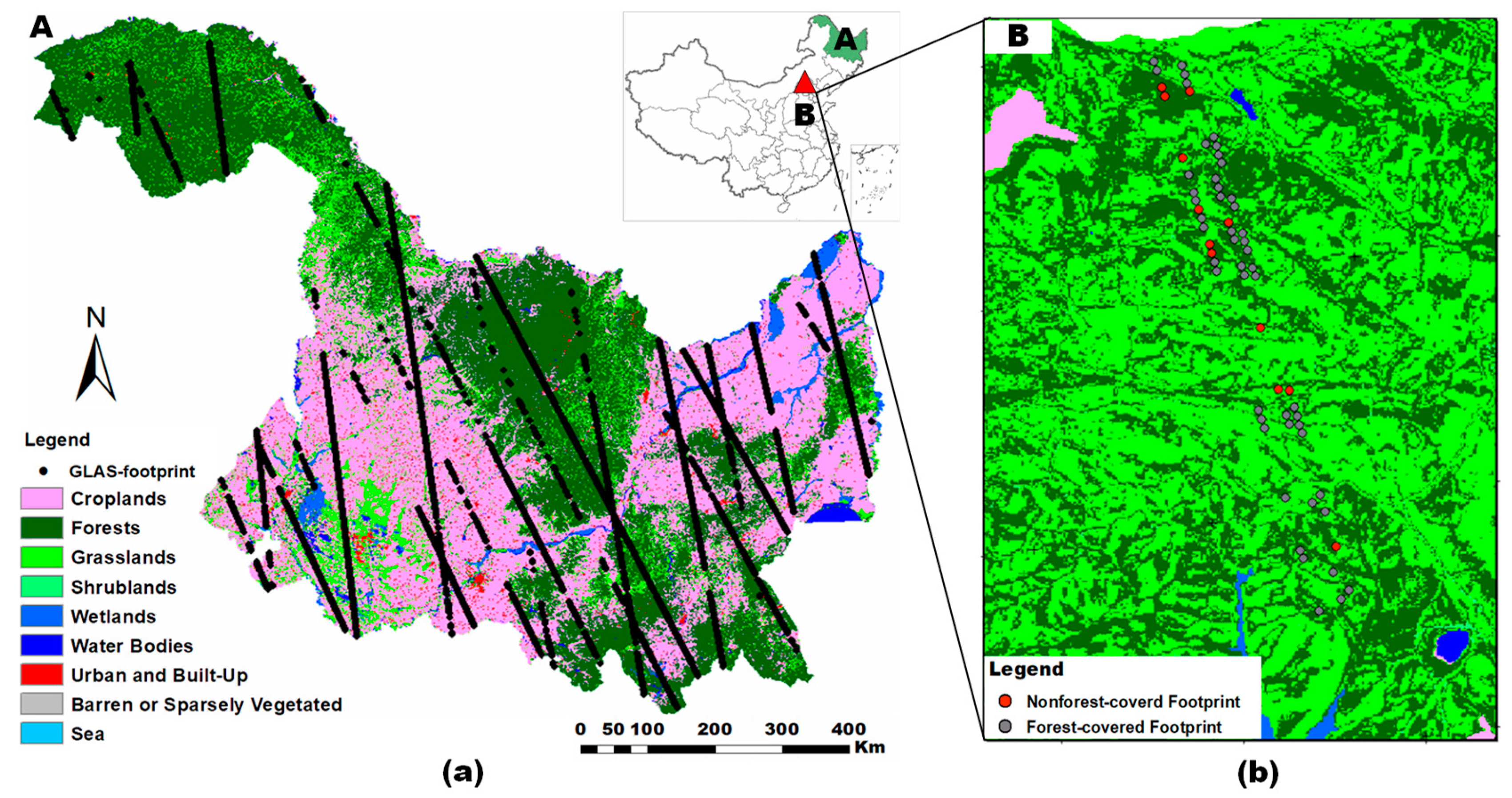
2.1. Study Area
2.2. Data used for Geoscience Laser Altimeter System (GLAS) Leaf Area Index (LAI) Inversion
2.2.1. Ice, Cloud and land Elevation Satellite (ICESat) GLAS Data
2.2.2. GlobeLand30 Landcover Data
2.2.3. Shuttle Radar Topography Mission (SRTM) Data
2.3. Moderate Resolution Imaging Spectroradiometer (MODIS) LAI Product
2.4. Ground-Based Data from Tracing Radiation and Architecture of Canopies (TRAC)
3. Models and Methods
3.1. Models
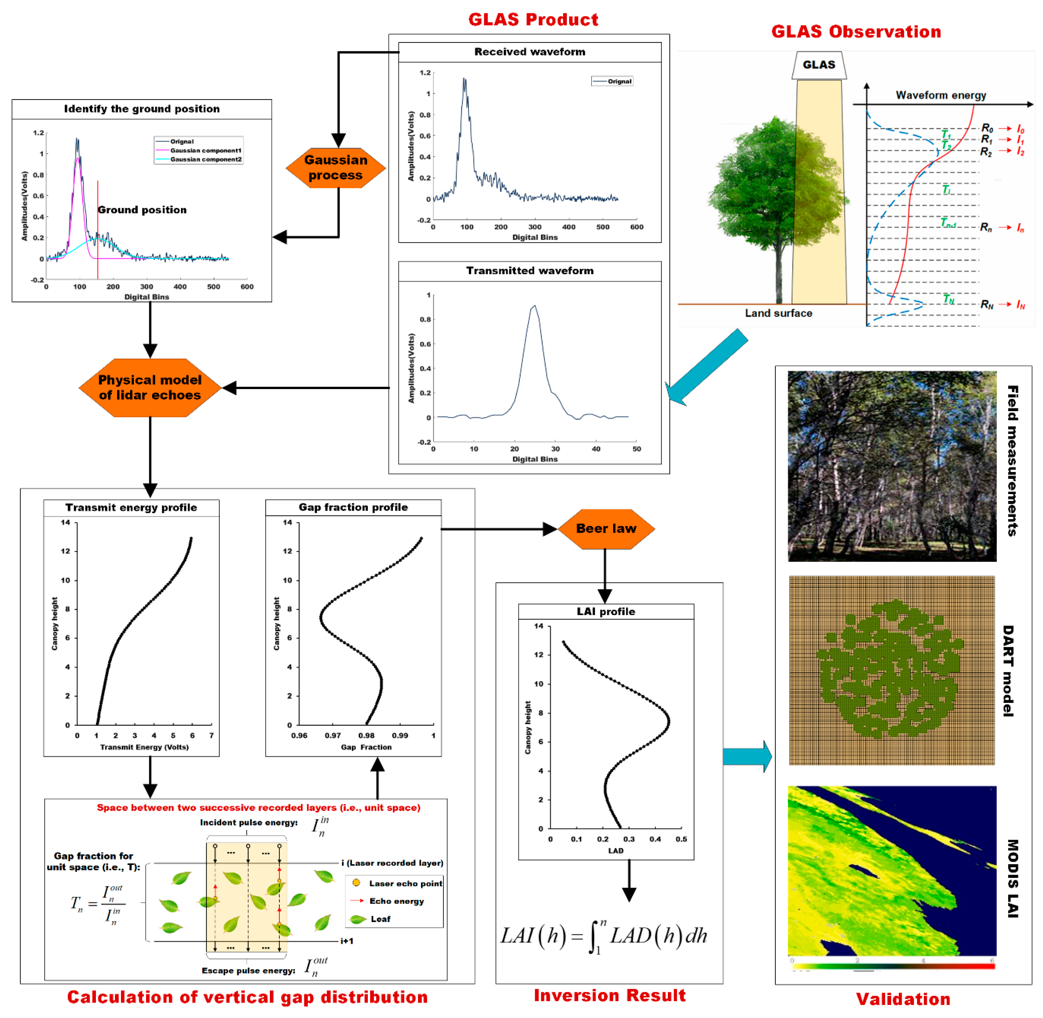
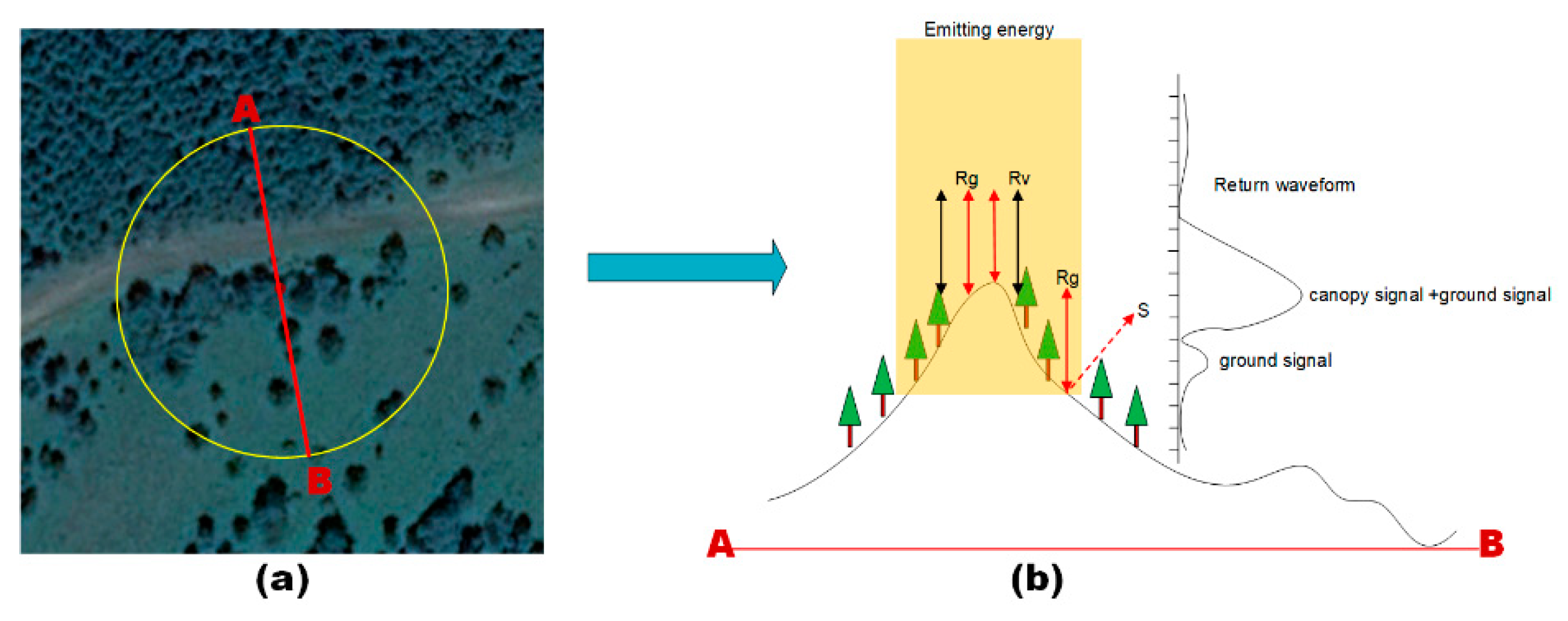
3.1.1. Physical Model of Light Detection and Ranging (Lidar) Echoes for Forest
3.1.2. Discrete Anisotropic Radiative Transfer (DART) Model
3.2. Methods
3.2.1. Vertical Foliage Profile (VFP) and LAI Calculation
3.2.2. Transmitted Energy Profile (TEP) Calculation
4. Results and Analysis
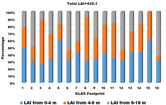
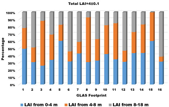
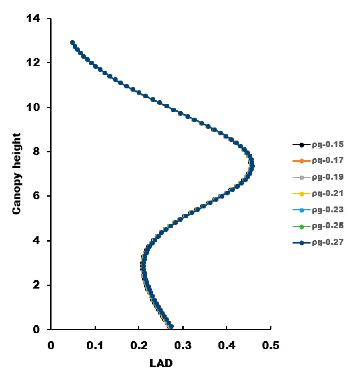
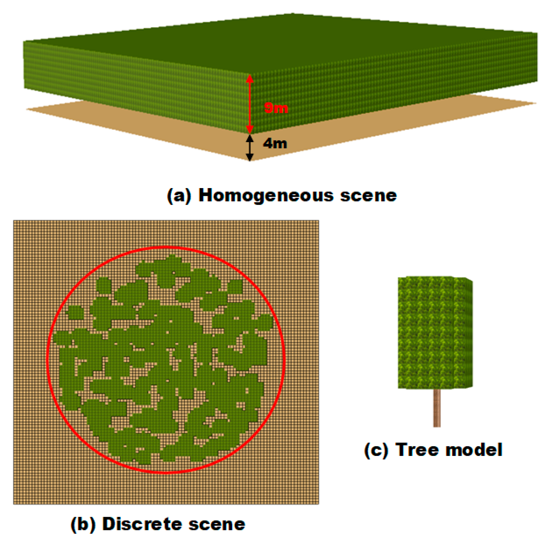
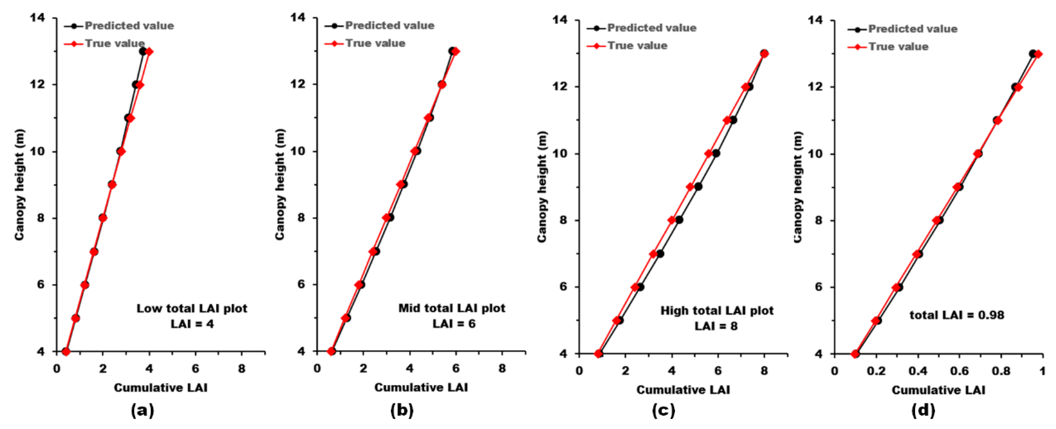
4.1. LAI Retrieval in Virtual Scenes
4.2. LAI Retrieval in Saihanba National Forest Park
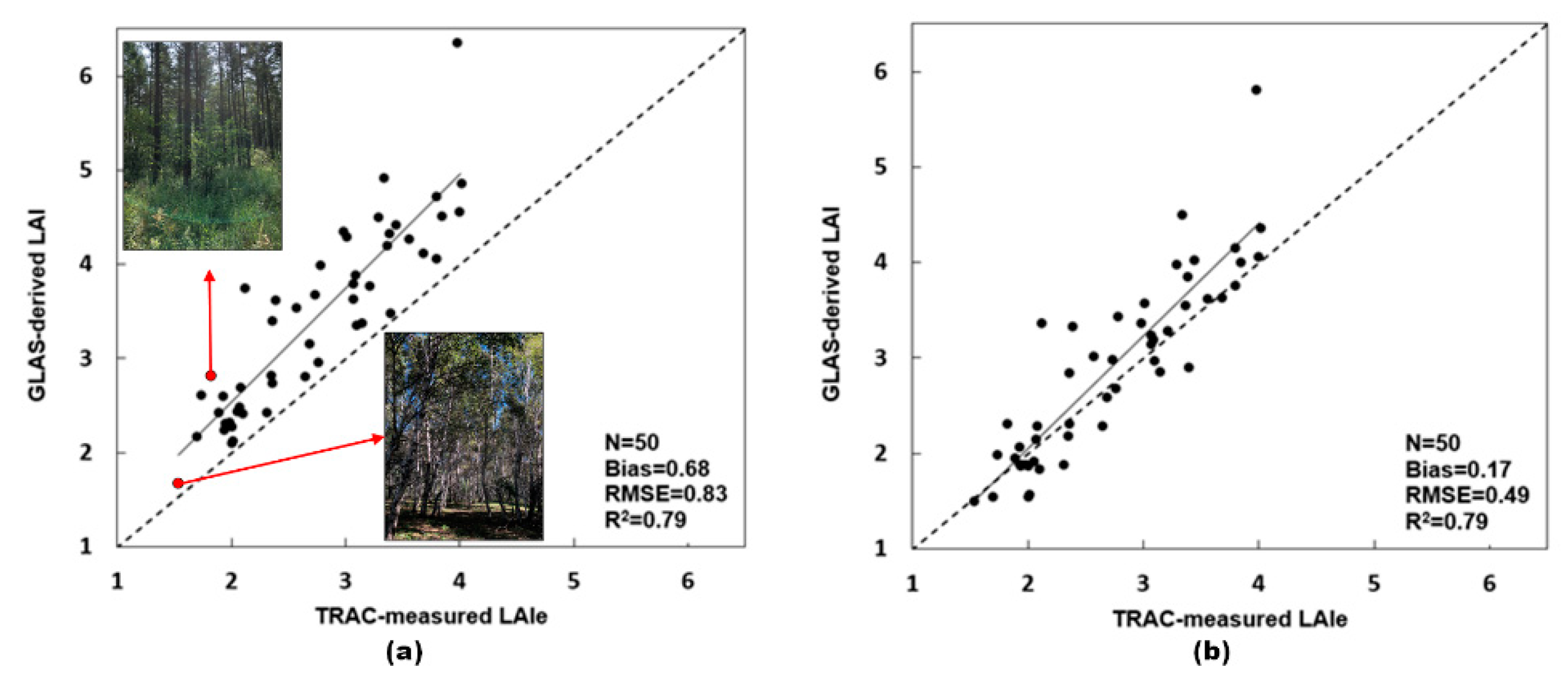
4.2.1. GLAS LAI vs. TRAC LAI
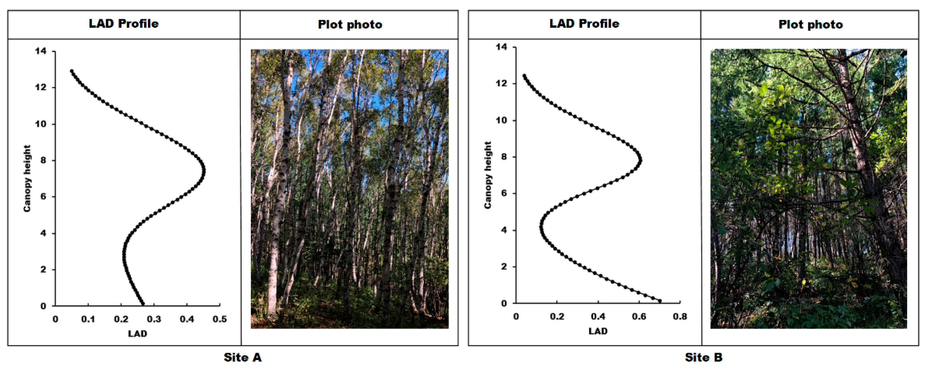
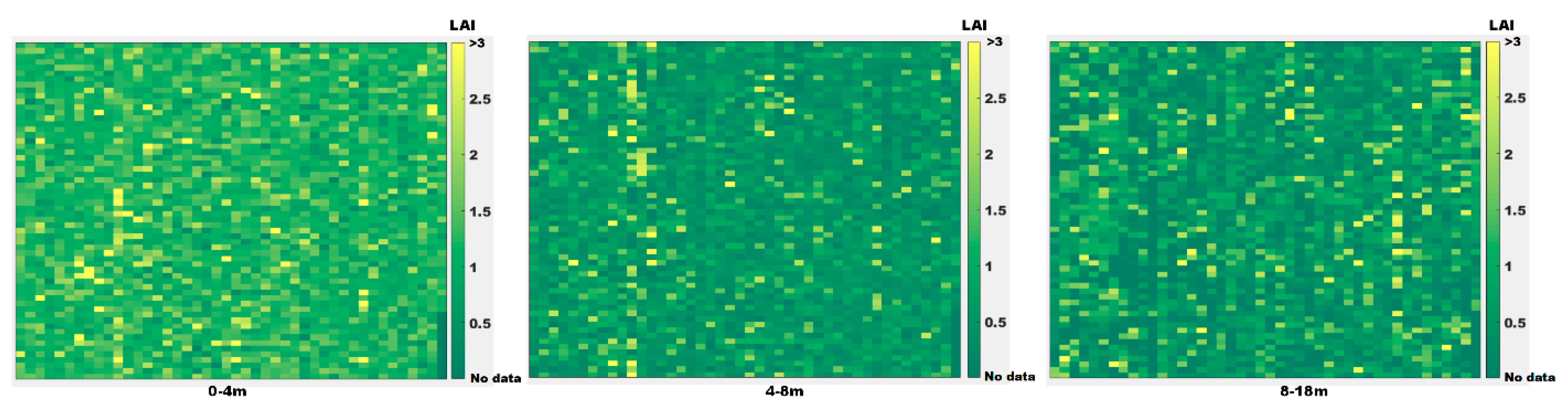
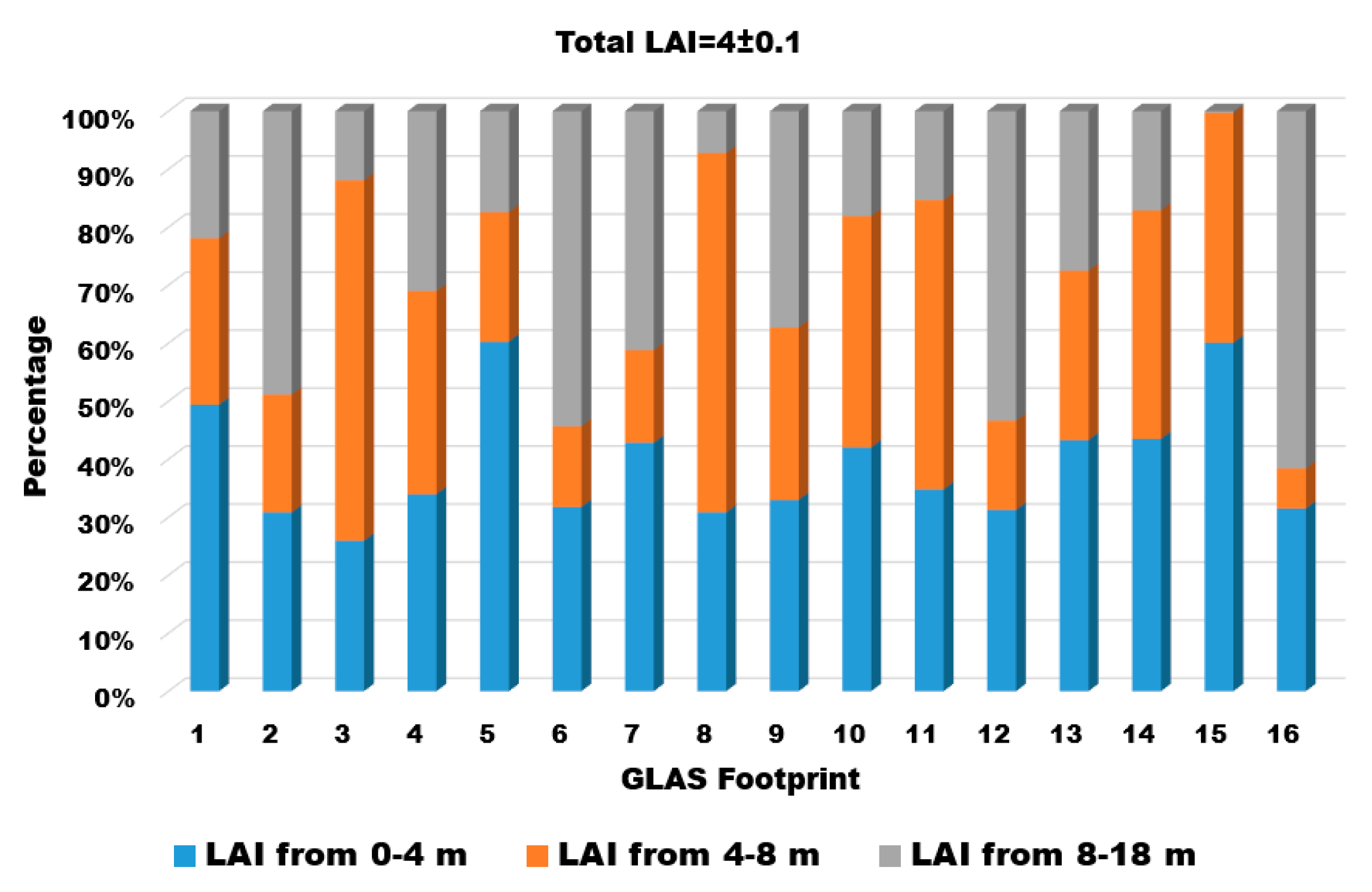
4.2.2. GLAS VFP Inversion
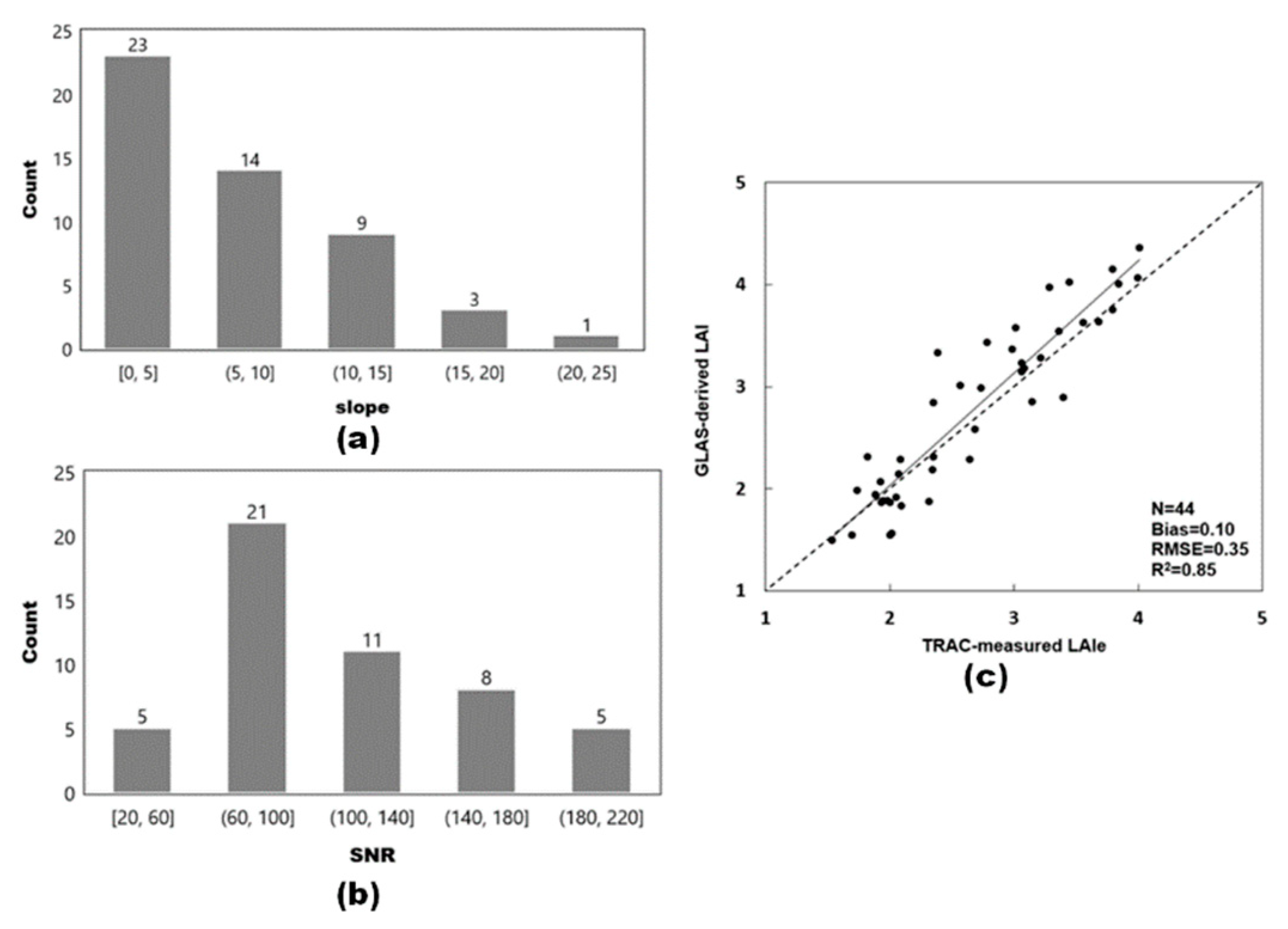
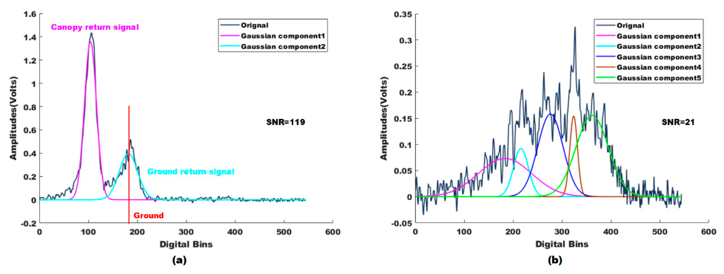
4.2.3. Uncertainty Analysis for Ground Validation
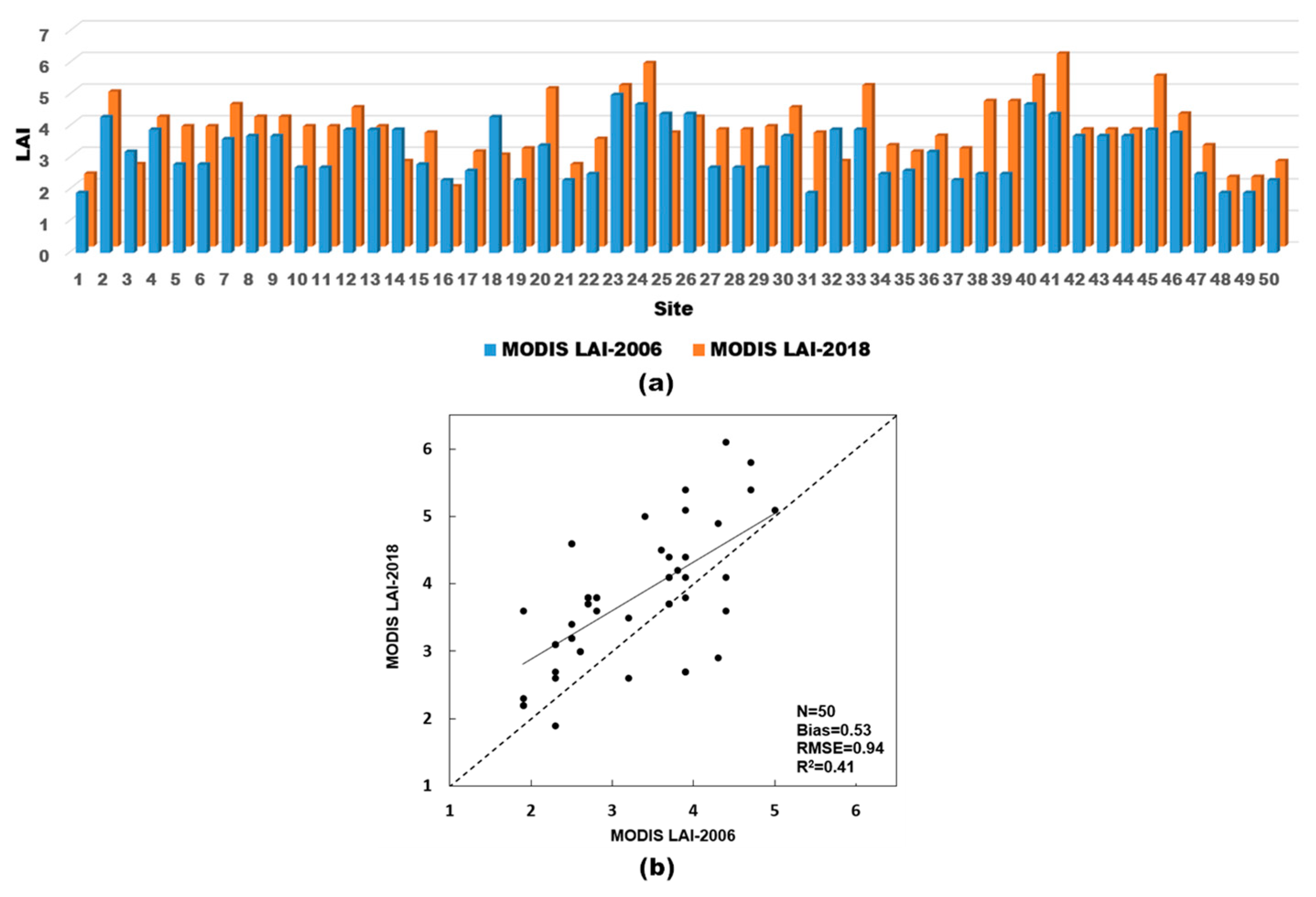
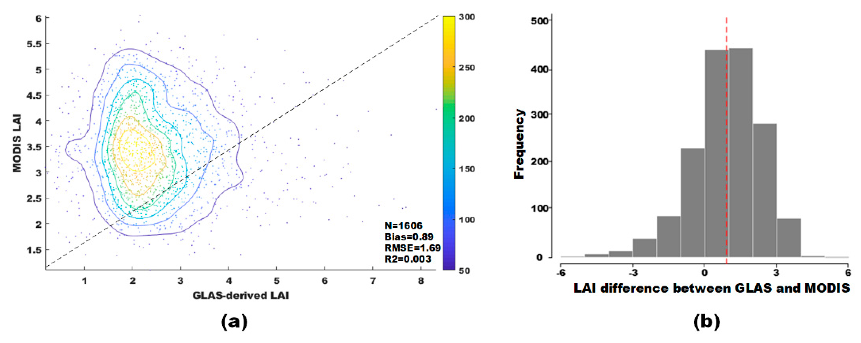
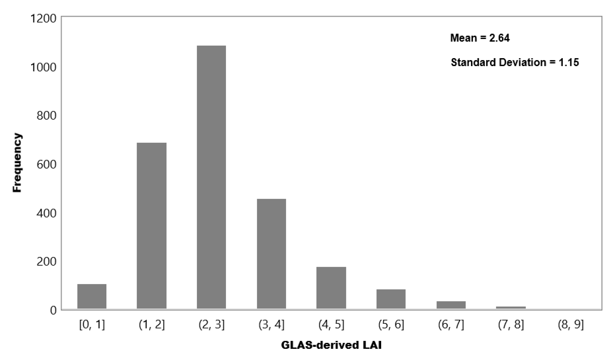
4.3. LAI Retrieval in Heilongjiang Province
GLAS LAI vs. MODIS LAI
4.4. Model Uncertainty Analysis
5. Discussion
6. Conclusions
Author Contributions
Funding
Conflicts of Interest
Appendix A

| Parameter | Symbol | Unit | Values |
|---|---|---|---|
| GLAS receiver calibration constant | α | dimensionless | Transmitted pulse: 1.21 Return pulse: 1.00 |
| Electronic throughput | dimensionless | 92.3% | |
| Optical throughput | dimensionless | Transmitted pulse: 2.97 × 10⁻¹⁴ for Laser 1, 2.79 × 10⁻¹⁴ for Laser 2, and 2.79 × 10⁻¹⁴ for Laser 3 Return pulse: 0.67 | |
| Detector responsibility | V/W | 2.28 × 10⁷ | |
| Variable gain amplifier (VGA) gain | G | dimensionless | Gtel/255, Gtel is an 8-b integer recorded in GLA05 product |
| Pulse waveform | W(i) | V | Transmitted pulse: r_tx_wf, which recorded in GLA01 product Return pulse: r_rng_wf, which recorded in GLA01 product. |
| Waveform sample numbers | N | dimensionless | Transmitted pulse: 48 Return pulse: 544. |
| Sample time of the receiver | △t | ns | 1 |
References
- Muiruri, E.W.; Barantal, S.; Iason, G.R.; Salminen, J.; Perez-Fernandez, E.; Koricheva, J. Forest diversity effects on insect herbivores: Do leaf traits matter? New Phytol. 2019, 221, 2250–2260. [Google Scholar] [CrossRef] [Green Version]
- Zhao, K.; Jackson, R.B. Biophysical forcings of land-use changes from potential forestry activities in North America. Ecol. Monogr. 2014, 84, 329–353. [Google Scholar] [CrossRef]
- Swantaran, A.; Dubayah, R.; Roberts, D.; Hofton, M.; Blair, J.B. Mapping biomass and stress in the Sierra Nevada using lidar and hyperspectral data fusion. Remote Sens. Environ. 2011, 115, 2917–2930. [Google Scholar] [CrossRef] [Green Version]
- Yan, G.; Hu, R.; Luo, J.; Weiss, M.; Jiang, H.; Mu, X.; Xie, D.; Zhang, W. Review of indirect optical measurements of leaf area index: Recent advances, challenges, and perspectives. Agric. For. Meteorol. 2019, 265, 390–411. [Google Scholar] [CrossRef]
- Parker, G.G.; Lefsky, M.; Harding, D. Light transmittance in forest canopies determined using airborne laser altimetry and in-canopy quantum measurements. Remote Sens. Environ. 2001, 76, 298–309. [Google Scholar] [CrossRef]
- Stark, S.C.; Leitold, V.; Wu, J.; Hunter, M.O.; De Castilho, C.V.; Costa, F.R.C.; McMahon, S.M.; Parker, G.G.; Shimabukuro, M.T.; Lefsky, M.A.; et al. Amazon forest carbon dynamics predicted by profiles of canopy leaf area and light environment. Ecol. Lett. 2012, 15, 1406–1414. [Google Scholar] [CrossRef] [PubMed] [Green Version]
- Chen, J.M.; Rich, P.M.; Gower, S.T.; Norman, J.M.; Plummer, S. Leaf area index of boreal forests: Theory, techniques, and measurements. J. Geophys. Res. Space Phys. 1997, 102, 29429–29443. [Google Scholar] [CrossRef]
- Myneni, R.B.; Hoffman, S.; Knyazikhin, Y.; Privette, J.L.; Glassy, J.; Tian, Y.; Wang, Y.; Song, X.; Zhang, Y.; Smith, G.R.; et al. Global products of vegetation leaf area and fraction absorbed PAR from year one of MODIS data. Remote Sens. Environ. 2002, 83, 214–231. [Google Scholar] [CrossRef] [Green Version]
- Morsdorf, F.; Kötz, B.; Meier, E.; Itten, K.; Allgöwer, B. Estimation of LAI and fractional cover from small footprint airborne laser scanning data based on gap fraction. Remote Sens. Environ. 2006, 104, 50–61. [Google Scholar] [CrossRef]
- Ganguly, S.; Schull, M.A.; Samanta, A.; Shabanov, N.V.; Milesi, C.; Nemani, R.R.; Knyazikhin, Y.; Myneni, R. Generating vegetation leaf area index earth system data record from multiple sensors. Part 1: Theory. Remote Sens. Environ. 2008, 112, 4333–4343. [Google Scholar] [CrossRef]
- Xiao, Z.; Liang, S.; Wang, J.; Chen, P.; Yin, X.; Zhang, L.; Song, J. Use of General Regression Neural Networks for Generating the GLASS Leaf Area Index Product from Time-Series MODIS Surface Reflectance. IEEE Trans. Geosci. Remote Sens. 2013, 52, 209–223. [Google Scholar] [CrossRef]
- He, B.; Li, X.; Quan, X.; Qiu, S. Estimating the Aboveground Dry Biomass of Grass by Assimilation of Retrieved LAI into a Crop Growth Model. IEEE J. Sel. Top. Appl. Earth Obs. Remote Sens. 2014, 8, 550–561. [Google Scholar] [CrossRef]
- Morisette, J.; Baret, F.; Privette, J.; Myneni, R.; Nickeson, J.; Garrigues, S.; Shabanov, N.V.; Weiss, M.; Fernandes, R.; Leblanc, S.; et al. Validation of global moderate-resolution LAI products: A framework proposed within the CEOS land product validation subgroup. IEEE Trans. Geosci. Remote Sens. 2006, 44, 1804–1817. [Google Scholar] [CrossRef] [Green Version]
- Xie, Q.; Huang, W.; Liang, N.; Chen, P.; Wu, C.; Yang, G.; Zhang, J.; Huang, L.; Zhang, N. Leaf Area Index Estimation Using Vegetation Indices Derived from Airborne Hyperspectral Images in Winter Wheat. IEEE J. Sel. Top. Appl. Earth Obs. Remote Sens. 2014, 7, 3586–3594. [Google Scholar] [CrossRef]
- Lei, C.; Jiao, Z.; Dong, Y.; Sun, M.; Zhang, X.; Yin, S.; Ding, A.; Chang, Y.; Guo, J.; Xie, R. Estimating Forest Canopy Height Using MODIS BRDF Data Emphasizing Typical-Angle Reflectances. Remote Sens. 2019, 11, 2239. [Google Scholar] [CrossRef] [Green Version]
- Dubayah, R.O.; Drake, J.B. Lidar Remote Sensing for Forestry. J. For. 2000, 98, 44–46. [Google Scholar]
- Zhao, K.; Suarez, J.; García, M.; Hu, T.; Wang, C.; Londo, A. Utility of multitemporal lidar for forest and carbon monitoring: Tree growth, biomass dynamics, and carbon flux. Remote Sens. Environ. 2018, 204, 883–897. [Google Scholar] [CrossRef]
- Tang, H.; Dubayah, R.; Swantaran, A.; Hofton, M.A.; Sheldon, S.; Clark, D.B.; Blair, B. Retrieval of vertical LAI profiles over tropical rain forests using waveform lidar at La Selva, Costa Rica. Remote Sens. Environ. 2012, 124, 242–250. [Google Scholar] [CrossRef]
- Ma, H.; Song, J.; Wang, J. Forest Canopy LAI and Vertical FAVD Profile Inversion from Airborne Full-Waveform LiDAR Data Based on a Radiative Transfer Model. Remote Sens. 2015, 7, 1897–1914. [Google Scholar] [CrossRef] [Green Version]
- Zhao, K.; García, M.; Liu, S.; Guo, Q.; Chen, G.; Zhang, X.; Zhou, Y.; Meng, X. Terrestrial lidar remote sensing of forests: Maximum likelihood estimates of canopy profile, leaf area index, and leaf angle distribution. Agric. For. Meteorol. 2015, 209, 100–113. [Google Scholar] [CrossRef]
- Hu, R.; Yan, G.; Mu, X.; Luo, J. Indirect measurement of leaf area index on the basis of path length distribution. Remote Sens. Environ. 2014, 155, 239–247. [Google Scholar] [CrossRef]
- Zhao, K.; Popescu, S.C. Lidar-based mapping of leaf area index and its use for validating GLOBCARBON satellite LAI product in a temperate forest of the southern USA. Remote Sens. Environ. 2009, 113, 1628–1645. [Google Scholar] [CrossRef]
- García, M.; Popescu, S.C.; Riaño, D.; Zhao, K.; Neuenschwander, A.; Agca, M.; Chuvieco, E. Characterization of canopy fuels using ICESat/GLAS data. Remote Sens. Environ. 2012, 123, 81–89. [Google Scholar] [CrossRef]
- Luo, S.; Wang, C.; Li, G.; Xi, X. Retrieving leaf area index using ICESat/GLAS full-waveform data. Remote Sens. Lett. 2013, 4, 745–753. [Google Scholar] [CrossRef]
- Tang, H.; Dubayah, R.; Brolly, M.; Ganguly, S.; Zhang, G. Large-scale retrieval of leaf area index and vertical foliage profile from the spaceborne waveform lidar (GLAS/ICESat). Remote Sens. Environ. 2014, 154, 8–18. [Google Scholar] [CrossRef]
- Tang, H.; Brolly, M.; Zhao, F.; Strahler, A.H.; Schaaf, C.; Ganguly, S.; Zhang, G.; Dubayah, R. Deriving and validating Leaf Area Index (LAI) at multiple spatial scales through lidar remote sensing: A case study in Sierra National Forest, CA. Remote Sens. Environ. 2014, 143, 131–141. [Google Scholar] [CrossRef]
- Yang, X.; Yang, X.; Pan, F.; Nie, S.; Xi, X.; Luo, S. Retrieving leaf area index in discontinuous forest using ICESat/GLAS full-waveform data based on gap fraction model. ISPRS J. Photogramm. Remote Sens. 2019, 148, 54–62. [Google Scholar] [CrossRef]
- Tian, J.; Wang, L.; Li, X.; Shi, C.; Gong, H. Differentiating Tree and Shrub LAI in a Mixed Forest with ICESat/GLAS Spaceborne LiDAR. IEEE J. Sel. Top. Appl. Earth Obs. Remote Sens. 2016, 10, 87–94. [Google Scholar] [CrossRef]
- North, P.; Rosette, J.; Suárez, J.C.; Los, S. A Monte Carlo radiative transfer model of satellite waveform LiDAR. Int. J. Remote Sens. 2010, 31, 1343–1358. [Google Scholar] [CrossRef]
- Brown, S.D.; Blevins, D.D.; Schott, J.R. Time-gated topographic LIDAR scene simulation. Def. Secur. 2005, 5791, 342–353. [Google Scholar]
- Govaerts, Y.; Verstraete, M. Raytran: A Monte Carlo ray-tracing model to compute light scattering in three-dimensional heterogeneous media. IEEE Trans. Geosci. Remote Sens. 1998, 36, 493–505. [Google Scholar] [CrossRef]
- Disney, M.; Lewis, P.; Bouvet, M.; Prieto-Blanco, A.; Hancock, S. Quantifying Surface Reflectivity for Spaceborne Lidar via Two Independent Methods. IEEE Trans. Geosci. Remote Sens. 2009, 47, 3262–3271. [Google Scholar] [CrossRef]
- Kobayashi, H.; Iwabuchi, H. A coupled 1-D atmosphere and 3-D canopy radiative transfer model for canopy reflectance, light environment, and photosynthesis simulation in a heterogeneous landscape. Remote Sens. Environ. 2008, 112, 173–185. [Google Scholar] [CrossRef]
- Gastellu, J.-P.; Yin, T.; Lauret, N.; Grau, E.; Rubio, J.; Cook, B.; Morton, D.; Sun, G. Simulation of satellite, airborne and terrestrial LiDAR with DART (I): Waveform simulation with quasi-Monte Carlo ray tracing. Remote Sens. Environ. 2016, 184, 418–435. [Google Scholar] [CrossRef]
- Yin, T.; Lauret, N.; Gastellu, J.-P. Simulation of satellite, airborne and terrestrial LiDAR with DART (II): ALS and TLS multi-pulse acquisitions, photon counting, and solar noise. Remote Sens. Environ. 2016, 184, 454–468. [Google Scholar] [CrossRef]
- Widlowski, J.-L.; Pinty, B.; Lopatka, M.; Atzberger, C.; Buzica, D.; Chelle, M.; Disney, M.; Gastellu, J.-P.; Gerboles, M.; Gobron, N.; et al. The fourth radiation transfer model intercomparison (RAMI-IV): Proficiency testing of canopy reflectance models with ISO-13528. J. Geophys. Res. Atmos. 2013, 118, 6869–6890. [Google Scholar] [CrossRef] [Green Version]
- Heilongjiang Forestry and Grassland Bureau. Available online: http://hljforest.com/ (accessed on 18 July 2020).
- Ting-ting, X.I.; Shun-long, L.I. Analysis of Forestry Carbon Mitigation Potential in Heilongjiang Province. Probl. For. Econ. 2006, 26, 519–522. [Google Scholar]
- Hebei Saihanba Mechanical Forestry Farm. Available online: http://www.saihanba.com.cn/ (accessed on 18 July 2020).
- Dong-zhi, W.; Hong-zhuo, M.I.; Dong-yan, Z.; Zhi-dong, Z.; Xuan-rui, H. Prediction of the Diameter Annual Radial Growth of Larix Principis-Rupprechtii and Betula Platyphylla Mixed Forest in Saihanba. J. Northwest For. Univ. 2017, 32, 1–6. [Google Scholar]
- Jun, C.; Ban, Y.; Li, S. Open Access to Earth Land-Cover Map. Nature 2014, 514, 434. [Google Scholar] [CrossRef] [Green Version]
- National Geomatics Center of China (NGCC). 30-Meter Global Land Cover Dataset (GlobeLand30)-Product Description Data. 2014. Available online: http://www.globallandcover.com/GLC30Download/index.aspx (accessed on 10 July 2019).
- Yan, K.; Park, T.; Yan, G.; Liu, Z.; Yang, B.; Chen, C.; Nemani, R.; Knyazikhin, Y.; Myneni, R. Evaluation of MODIS LAI/FPAR Product Collection 6. Part 2: Validation and Intercomparison. Remote Sens. 2016, 8, 460. [Google Scholar] [CrossRef] [Green Version]
- Chen, J.M.; Cihlar, J. Plant canopy gap-size analysis theory for improving optical measurements of leaf-area index. Appl. Opt. 1995, 34, 6211–6222. [Google Scholar] [CrossRef] [PubMed] [Green Version]
- Gastellu, J.-P.; Demarez, V.; Pinel, V.; Zagolski, F. Modeling radiative transfer in heterogeneous 3-D vegetation canopies. Remote Sens. Environ. 1996, 58, 131–156. [Google Scholar] [CrossRef] [Green Version]
- Baldocchi, D.D.; Hutchison, B.A.; Matt, D.R.; McMillen, R.T. Canopy Radiative Transfer Models for Spherical and Known Leaf Inclination Angle Distributions: A Test in an Oak-Hickory Forest. J. Appl. Ecol. 1985, 22, 539. [Google Scholar] [CrossRef]
- Sun, X.; Abshire, J.B.; Borsa, A.A.; Fricker, H.A.; Yi, D.; DiMarzio, J.P.; Paolo, F.S.; Brunt, K.M.; Harding, D.J.; Neumann, G.A. ICESAT/GLAS Altimetry Measurements: Received Signal Dynamic Range and Saturation Correction. IEEE Trans. Geosci. Remote Sens. 2017, 55, 5440–5454. [Google Scholar] [CrossRef]
- Nie, S.; Wang, C.; Li, G.; Pan, F.; Xi, X.; Luo, S. Signal-to-noise ratio–based quality assessment method for ICESat/GLAS waveform data. Opt. Eng. 2014, 53, 103104. [Google Scholar] [CrossRef]
- Hayashi, M.; Saigusa, N.; Oguma, H.; Yamagata, Y. Forest canopy height estimation using ICESat/GLAS data and error factor analysis in Hokkaido, Japan. ISPRS J. Photogramm. Remote Sens. 2013, 81, 12–18. [Google Scholar] [CrossRef]
- Hilbert, C.; Schmullius, C. Influence of Surface Topography on ICESat/GLAS Forest Height Estimation and Waveform Shape. Remote Sens. 2012, 4, 2210–2235. [Google Scholar] [CrossRef] [Green Version]
- KelleriD, M.; Lefsky, M.A.; Pang, Y.; De Camargo, P.B.; Hunter, M. Revised method for forest canopy height estimation from Geoscience Laser Altimeter System waveforms. J. Appl. Remote Sens. 2007, 1, 013537. [Google Scholar] [CrossRef]
- Pang, Y.; Li, Z.; Lefsky, M.; Guoqing, S.; Yu, X. Model Based Terrain Effect Analyses on ICEsat GLAS Waveforms. In Proceedings of the 2006 IEEE International Symposium on Geoscience and Remote Sensing, Denver, CO, USA, 31 July–4 August 2006; p. 3232. [Google Scholar]
- Wang, X.; Huang, H.; Gong, P.; Liu, C.; Li, C.; Li, W. Forest Canopy Height Extraction in Rugged Areas with ICESat/GLAS Data. IEEE Trans. Geosci. Remote Sens. 2013, 52, 4650–4657. [Google Scholar] [CrossRef]
- Wang, M.; Sun, R.; Xiao, Z. Estimation of Forest Canopy Height and Aboveground Biomass from Spaceborne LiDAR and Landsat Imageries in Maryland. Remote Sens. 2018, 10, 344. [Google Scholar] [CrossRef] [Green Version]
- Huang, D.; Knyazikhin, Y.; Dickinson, R.E.; Rautiainen, M.; Stenberg, P.; Disney, M.; Lewis, P.; Cescatti, A.; Tian, Y.; Verhoef, W.; et al. Canopy spectral invariants for remote sensing and model applications. Remote Sens. Environ. 2007, 106, 106–122. [Google Scholar] [CrossRef] [Green Version]
- Knyazikhin, Y.; Martonchik, J.V.; Myneni, R.; Diner, D.J.; Running, S.W. Synergistic algorithm for estimating vegetation canopy leaf area index and fraction of absorbed photosynthetically active radiation from MODIS and MISR data. J. Geophys. Res. Space Phys. 1998, 103, 32257–32275. [Google Scholar] [CrossRef] [Green Version]
- Jensen, J.L.; Humes, K.S.; Vierling, L.A.; Hudak, A.T. Discrete return lidar-based prediction of leaf area index in two conifer forests. Remote Sens. Environ. 2008, 112, 3947–3957. [Google Scholar] [CrossRef] [Green Version]
- Jiao, Z.; Zhang, X.; Bréon, F.-M.; Dong, Y.; Schaaf, C.B.; Roman, M.; Wang, Z.; Cui, L.; Yin, S.; Ding, A.; et al. The influence of spatial resolution on the angular variation patterns of optical reflectance as retrieved from MODIS and POLDER measurements. Remote Sens. Environ. 2018, 215, 371–385. [Google Scholar] [CrossRef]
- Jiao, Z.; Dong, Y.; Schaaf, C.B.; Chen, J.M.; Roman, M.; Wang, Z.; Zhang, H.; Ding, A.; Erb, A.; Hill, M.J.; et al. An algorithm for the retrieval of the clumping index (CI) from the MODIS BRDF product using an adjusted version of the kernel-driven BRDF model. Remote Sens. Environ. 2018, 209, 594–611. [Google Scholar] [CrossRef]
- Dong, Y.; Jiao, Z.; Yin, S.; Zhang, H.; Zhang, X.; Lei, C.; He, D.; Ding, A.; Chang, Y.; Yang, S. Influence of Snow on the Magnitude and Seasonal Variation of the Clumping Index Retrieved from MODIS BRDF Products. Remote Sens. 2018, 10, 1194. [Google Scholar] [CrossRef] [Green Version]
- Jiao, Z.; Schaaf, C.; Dong, Y.; Román, M.; Hill, M.J.; Chen, J.M.; Wang, Z.; Zhang, H.; Saenz, E.; Poudyal, R.; et al. A method for improving hotspot directional signatures in BRDF models used for MODIS. Remote Sens. Environ. 2016, 186, 135–151. [Google Scholar] [CrossRef] [Green Version]
- Dong, Y.; Jiao, Z.; Cui, L.; Zhang, H.; Zhang, X.; Yin, S.; Ding, A.; Chang, Y.; Xie, R.; Guo, J. Assessment of the Hotspot Effect for the PROSAIL Model with POLDER Hotspot Observations Based on the Hotspot-Enhanced Kernel-Driven BRDF Model. IEEE Trans. Geosci. Remote Sens. 2019, 57, 8048–8064. [Google Scholar] [CrossRef]
- Chen, J.M.; Menges, C.; Leblanc, S. Global mapping of foliage clumping index using multi-angular satellite data. Remote Sens. Environ. 2005, 97, 447–457. [Google Scholar] [CrossRef]
- Pinker, R.T.; Stowe, L.L. Modelling planetary bidirectional reflectance over land. Int. J. Remote Sens. 1990, 11, 113–123. [Google Scholar] [CrossRef]
- Liang, S. A direct algorithm for estimating land surface broadband albedos from MODIS imagery. IEEE Trans. Geosci. Remote Sens. 2003, 41, 136–145. [Google Scholar] [CrossRef]
- Nilsson, M.C.; Wardle, D.A. Understory Vegetation as a Forest Ecosystem Driver: Evidence from the Northern Swedish Boreal Forest. Front. Ecol. Environ. 2005, 3, 421–428. [Google Scholar] [CrossRef]
- Kotchenova, S.Y.; Song, X.; Shabanov, N.V.; Potter, C.S.; Knyazikhin, Y.; Myneni, R. Lidar remote sensing for modeling gross primary production of deciduous forests. Remote Sens. Environ. 2004, 92, 158–172. [Google Scholar] [CrossRef]
- Sprintsin, M.; Chen, J.M.; Desai, A.R.; Gough, C.M. Evaluation of leaf-to-canopy upscaling methodologies against carbon flux data in North America. J. Geophys. Res. Space Phys. 2012, 117. [Google Scholar] [CrossRef] [Green Version]


| Parameter | Unit | Values |
|---|---|---|
| Pulse energy | mJ | 73 |
| Half pulse duration | dimensionless | 6 |
| Lidar acquisition rate | ns | 1 |
| Wavelength | nm | 1064 |
| Bandwidth | ns | 0.08 |
| Area of lidar sensor | m2 | 0.785 |
| Effective telescope diameter | m | 0.95 |
| Sensor altitude | km | 600 |
| Footprint radius | m | 35 |
| Field of view (FOV) radius | m | 48 |
| Parameter | Symbol | Unit | Values |
|---|---|---|---|
| Optics transmission | dimensionless | 0.67 | |
| Telescope area | m2 | 0.709 | |
| Roundtrip atmosphere transmission | dimensionless | is equal to the value of “d_reflCor_atm”. | |
| Range between GLAS sensor and ground | D | m | where C is the light transmission speed. |
| GLAS sensor emitted total pulse energy | J | I0 is calculated from the GLAS transmitted waveform recorded in the GLAS product (i.e., r_tx_wf), and the calculation details are shown in the Appendix A. | |
| GLAS sensor received echo energy at each recorded layer | Ri | J | Ri is calculated from the GLAS received waveform recorded in the GLAS product (i.e., r_rng_wf), and the calculation details are shown in the Appendix A. |
© 2020 by the authors. Licensee MDPI, Basel, Switzerland. This article is an open access article distributed under the terms and conditions of the Creative Commons Attribution (CC BY) license (http://creativecommons.org/licenses/by/4.0/).
Share and Cite
Cui, L.; Jiao, Z.; Zhao, K.; Sun, M.; Dong, Y.; Yin, S.; Li, Y.; Chang, Y.; Guo, J.; Xie, R.; et al. Retrieval of Vertical Foliage Profile and Leaf Area Index Using Transmitted Energy Information Derived from ICESat GLAS Data. Remote Sens. 2020, 12, 2457. https://doi.org/10.3390/rs12152457
Cui L, Jiao Z, Zhao K, Sun M, Dong Y, Yin S, Li Y, Chang Y, Guo J, Xie R, et al. Retrieval of Vertical Foliage Profile and Leaf Area Index Using Transmitted Energy Information Derived from ICESat GLAS Data. Remote Sensing. 2020; 12(15):2457. https://doi.org/10.3390/rs12152457
Chicago/Turabian StyleCui, Lei, Ziti Jiao, Kaiguang Zhao, Mei Sun, Yadong Dong, Siyang Yin, Yang Li, Yaxuan Chang, Jing Guo, Rui Xie, and et al. 2020. "Retrieval of Vertical Foliage Profile and Leaf Area Index Using Transmitted Energy Information Derived from ICESat GLAS Data" Remote Sensing 12, no. 15: 2457. https://doi.org/10.3390/rs12152457