Climatology of Planetary Boundary Layer Height-Controlling Meteorological Parameters Over the Korean Peninsula


Korea Institute of Civil Engineering and Building Technology, Ilsan 10223, Korea
*
Author to whom correspondence should be addressed.
Remote Sens. 2020, 12(16), 2571; https://doi.org/10.3390/rs12162571
Submission received: 21 July 2020
/
Accepted: 6 August 2020
/
Published: 10 August 2020
(This article belongs to the Special Issue Remote Sensing for Climate Change Studies)
Abstract
:Planetary boundary layer (PBL) height plays a significant role in climate modeling, weather forecasting, air quality prediction, and pollution transport processes. This study examined the climatology of PBL-associated meteorological parameters over the Korean peninsula and surrounding sea using data from the ERA5 dataset produced by the European Centre for Medium-range Weather Forecasts (ECMWF). The data covered the period from 2008 to 2017. The bulk Richardson number methodology was used to determine the PBL height (PBLH). The PBLH obtained from the ERA5 data agreed well with that derived from sounding and Global Positioning System Radio Occultation datasets. Significant diurnal and seasonal variability in PBLH was observed. The PBLH increases from morning to late afternoon, decreases in the evening, and is lowest at night. It is high in the summer, lower in spring and autumn, and lowest in winter. The variability of the PBLH with respect to temperature, relative humidity, surface pressure, wind speed, lower tropospheric stability, soil moisture, and surface fluxes was also examined. The growth of the PBLH was high in the spring and in southern regions due to the low soil moisture content of the surface. A high PBLH pattern is evident in high-elevation regions. Increasing trends of the surface temperature and accordingly PBLH were observed from 2008 to 2017.
1. Introduction
The planetary boundary layer (PBL) is the lowest portion of the troposphere and is directly influenced by the Earth’s surface forcings over short periods of time (1 h or less) [1,2]. The exchange processes between the Earth and the atmosphere play a crucial role in the development of the PBL. PBL patterns are also influenced by atmospheric conditions, topographic features, and land use. The vertical transport of heat, momentum, moisture, turbulence, and air pollutants between the Earth’s surface and free atmosphere take place via the PBL. Thus, the PBL plays an important role in the occurrence of extreme weather events and is used in numerical weather prediction models.
The PBL structure can be estimated using the datasets of various in situ remote sensing tools, such as radio detection and ranging (RADAR), sound detection and ranging (SODAR), light detection and ranging (LIDAR), and radiosonde [3,4,5,6,7,8]. However, in situ instruments cannot adequately cover some areas (e.g., oceans, mountains, and deserts). Thus, satellite and reanalysis datasets are used to describe PBL characteristics around the world. Several researchers [9,10,11,12,13,14,15,16] have developed methods for estimating PBL height (PBLH) using reanalysis and radiosonde datasets. Seidel et al. [13] described the global climatology of the PBL over a 10-years period using 505 sonde datasets. They used seven methods to compute PBLH from various atmospheric parameters. They also evaluated the effect of uncertainty in the parameters on PBL estimation. Subsequently, Seidel et al. [14] studied PBL climatology over the continental United States and Europe using radiosonde, ERA, and climate model datasets for a 2 years period (ERA stands for “ECMWF Re-Analysis” and refers to a series of research projects conducted at the European Centre for Medium-range Weather Forecasts (ECMWF), which have produced the ERA-Interim, ERA-40, ERA-5, and various other datasets). The properties of the PBL over oceans were studied by Guo et al. [17] using global positioning system radio occultation (GPSRO) data for a 1 year period. The authors validated the PBLH determined from the GPSRO data by comparison with radiosonde and ECMWF data measurements. They demonstrated that the spatial and temporal variability of the PBL estimated from the GPSRO data was consistent with that estimated from the ECMWF data. The PBL climatology over land, ocean, and desert regions was described by von Engeln and Teixeira [15] and Basha et al. [12] using ECMWF and GPSRO observations, respectively. These researchers also examined the PBL structure over the inter-tropical convergence zone.
PBL characteristics over mountainous terrain differ significantly from those over plain regions. Orographic forcing, wind speed, convection, air pollution transport, and momentum exchange processes are more pronounced over mountainous terrain. Few studies have examined PBL characteristics over complex topographies. De Wekker et al. [18] found that the PBLH over mountainous terrain varies with terrain elevation. They also found that the presence of a deep mixing layer over these high elevation regions is caused by vigorous mixing of thermals and is associated with high aerosol layer heights. Lieman and Alpert [19] observed that the displacement/convergence of thermal ridges over mountains produces strong mixed layers that influence the dispersion of air pollutants and create a high PBLH. Kalthoff et al. [20] found a correlation between convective boundary layer (CBL) growth and orography. They reported that CBL growth follows the shape of orography because of the strong horizontal gradients of moisture and pollutants. De Wekker and Kossmann [21] reviewed the variability of PBLH over mountainous terrain and reported that CBL height differs significantly over slopes, valleys and basins, and plateaus and mountain ridges. They also found that thermally induced upslope winds increase CBL height. Bulging of the CBL height occurred at higher elevations as a result of upslope winds, heating of slopes and ridge tops, and strong convection. They concluded that the evolution of the CBL is closely related to a complex terrain wind system that contributes to the vertical transport/mixing of air pollutants.
The PBL structure over the Korean peninsula differs significantly from that over other regions because of the peninsula’s complex topography. The topography of the Korean peninsula is illustrated in Figure 1. Approximately 70% of the land area of Korea is occupied by mountains, especially concentrated in the northeast. The peninsula is bordered by the East Sea, Yellow Sea, and East China Sea to the east, west, and south, respectively. This complex topography substantially impacts the PBL via orography and sea breezes. Very few studies have focused on characterizing the PBL pattern over this region. The PBLH over South Korea has been estimated using radiosonde [22], LIDAR [23], and wind profiler [24] data as well as with a regional model [25]. Lee and Kawai [24] computed the mixing layer (ML) height from the range-corrected signal-to-noise ratio (RCSNR) of wind profilers for two sites (Munsan and Gangneung) in a case study. A new data transfer method was proposed by Lee et al. [25] to calculate the ML height from the virtual potential temperature (VPT), water vapor mixing ratio (MX), and relative humidity (RH) of sounding datasets for two sites (Osan and Gwangju) collected over a 1-year period. The elevated (summer) and depressed (winter) ML heights obtained were attributed to high and low skin temperatures, respectively. The spatial and temporal variability of the PBL over South Korea was studied by Lee et al. [26] using regional grid model data. They described the morning growth rate of the ML and maximum daytime ML height for a period of 1 year.
The reported studies over the Korean peninsula have selected only limited (two or three) sites to study PBL characteristics. Furthermore, these studies considered only short time durations (approximately 1 year), and the reasons for the spatial and temporal variability of the PBL were not extensively described. Therefore, it is difficult to define any detailed pattern or climatology of the PBLH over this region based on these studies. Thus, considering this aspect, the present study focuses on the following objectives: (i) comprehensively examine the characteristics of the PBL over the entire Korean peninsula (south and north) over a 10 years period (2008–2017) using high-resolution ERA5 datasets; (ii) describe the spatial and temporal variability of the PBL and its relation (controlling factors) with various atmospheric parameters; (iii) examine the patterns of diurnal and seasonal variations and orographic modification of the PBL, and further, latitudinal variation of the PBLH with respect to various atmospheric controlling factors is also described; (iv) examine how the soil moisture influences the PBLH growth during different seasons; (v) describe the variability of surface temperature, and accordingly PBLH, for the 10-years period; and (vi) validate the PBLH derived from the ERA datasets against the PBLH determined from the sounding and GPSRO datasets.
The remainder of this paper is organized as follows. The data and methods used to estimate the PBLH are presented in Section 2. The diurnal, seasonal, and orographic variabilities, as well as the growth rate of the PBL, are discussed in Section 3. The variability of PBLH for the 10 years period from 2008 to 2017 is also described in Section 3. Finally, a summary and conclusions are presented in Section 4.
2. Data and Methods
2.1. Meteorological Data
The ERA5 and radiosonde datasets were used to describe the PBL climatology of the Korean peninsula (~32–43°N, 123–131°E) from 2008 to 2017. The ERA5 is the fifth generation ECMWF atmospheric reanalysis of the global climate, which was produced by assimilating several satellite and radiosonde observational datasets [27]. It also includes various observational datasets obtained from the World Meteorological Organization’s Global Telecommunication System (GTS). It covers the entire global atmosphere and provides spatial and temporal data products. ERA5 data has a 0.25° × 0.25° grid horizontal resolution and a height resolution of 37 pressure levels with hourly temporal resolution. ERA captures the boundary layer reasonably well with these resolutions [14]. We used data from 2008–2017 to characterize the PBL climatology. Vertical profiles of the temperature (T), potential temperature (PT), virtual potential temperature (VPT), relative humidity (RH), specific humidity (SH), refractivity (N), and water vapor mixing ratio (MX) as well as the surface parameters of the T, RH, pressure (P), 10 m wind speed (WS), lower tropospheric stability (LTS), and ozone mixing ratio were derived from the ERA data to describe PBL characteristics. The difference between the PT at 700 hPa and surface PT values reflects the LTS [28]. The surface flux (latent and sensible) data were collected from MERRA-2 (not available from ERA) to relate with the PBLH. Further, the Bowen ratio (ratio between surface sensible heat flux and latent heat flux) was derived to describe the soil moisture, absorption, and evaporation of the solar radiation that influences the PBLH.
We used sounding data to validate the PBLH derived from ERA5. The University of Wyoming provides sounding data collected worldwide, typically two or four times a day. The T, PT, VPT, RH, mixing ratio (MR), and P profiles were obtained from this sounding data; profiles of N and SH were derived for use in estimating the PBLH. This provides data at various resolutions at specified heights on each day. The sounding data are only available for four locations (Osan, Gwangju, Gangneung, and Pohang) over the Korean peninsula; therefore, we used these four sites for the validation. We discarded the erroneous and rainy datasets to maintain quality control over the data. Further, to validate the ERA PBLH throughout the Korean peninsula, we used the Constellation Observing System for Meteorology, Ionosphere, and Climate (COSMIC) GPSRO measurements. The COSMIC GPSRO measurements provide the parameters of temperature, water vapor, refractivity, and bending angle profiles. Several studies have used GPSRO measurements for PBLH estimation [12,15,29], and inferred that the GPSRO estimated the PBLH reasonably well.
2.2. Methods to Determine PBLH
Various methods have been described in previous studies to estimate the PBLH. For the sake of completeness, these methods are briefly described here. PT is a combination of P and T and represents the static stability of the atmosphere. It also affects the adiabatic change of air parcels and air pollutant dispersion. The maximum gradient of the PT indicates the mixing height (PBLH), which signifies the transition from a convectively less stable (lower) region to a more stable (upper) region. The VPT is the potential temperature that dry air should have to possess the same density as moist air. It considers the moisture and temperature to represent buoyancy and stability. The maximum gradient of the VPT signifies the mixing of warm air parcels with the surrounding air (PBLH) and provides atmospheric buoyancy information [14,15]. RH is a function of the water vapor content and temperature. It is a measure of the amount of water vapor in the air compared to the total amount that can exist at the current temperature. The minimum gradient of RH is an indicator of the height of the PBL top, which refers to the top of the cloud layer [15]. Specific humidity (SH) is the mass of water vapor per unit mass of moist air. The minimum gradient of SH indicates the PBLH. The MR is the ratio of the mass of water vapor to the mass of dry air. It decreases with the mixing of dry air and moist air. Thus, the minimum gradient of the MR is an indicator of the PBLH. Refractivity (N) is a function of P, T, and RH and is thus sensitive to variations in all three parameters. The minimum N is an indicator of the PBLH.
Some of the above methods may estimate the PBLH under turbulent and strong solar conditions. However, it has recently been proven that the bulk Richardson number (Ri) method is suitable for studying PBL climatology [14,30]. Further, it is adequate for both stable and convective boundary layers and thus can be used for sounding and reanalysis datasets. Therefore, in the present study, we used a Ri-based methodology [31] to estimate the PBLH. Ri values ranging from 0.2 to 0.3 were used for the PBLH estimation. We tested different Ri values and selected 0.25 as the critical value for PBLH estimation and compared it with the sounding datasets. Ri is defined as:
where g is the acceleration due to gravity, z is the height (m), s represents the surface, θv is the virtual potential temperature, and u and v are the wind speed components. The height level that exceeds or corresponds to the critical value 0.25 of Ri represents the PBLH. To avoid noisy data and overestimated PBLH values, we used data ranging between 10 m and 4 km for accurate PBLH estimation [30]. Thus, the cases related to deep convection that produce high PBLH (>4 km) may not be included. Initially, we estimated the hourly PBLH for each day for all ten years of data. Then, we computed the mean PBLH for each month to obtain the monthly diurnal cycle. Further, to obtain the seasonal cycles, the corresponding months were averaged over hourly snapshots: (1) December, January, and February for winter; (2) March, April, and May for spring; (3) June, July, and August for summer; and (4) September, October, and November for autumn. Similarly, the surface parameters were also averaged seasonally for all ten years of data.
3. Results and Discussion
The PBLH above ground level was estimated using the method described above. We validated the PBLH values estimated from the ERA data with those derived from the sounding measurements using the bulk Richardson number methodology. Figure 2a shows the scatter plots between ERA PBLH and radiosonde PBLH over four different geographical locations (Osan, Gwangju, Pohang, and Gangneung). The days with rain, severe convection, and erroneous data were discarded from the comparison to maintain quality control over the data. On some days, the sounding data are also not available. The 15-local time (LT = Universal Time UT + 09:00) data of the ERA and sounding were considered for comparison. The elevations of Osan and Gwangju are 0 m above ground level (agl). The Pohang and Gangneung stations are at 300 m and ~1200 m agl, respectively. The elevation of Gangneung is higher than those of other stations. The top left panel corresponds to the Osan station, which shows that the correlation between ERA and radiosonde is 0.78 with a standard deviation of 0.19. A total of 223 soundings were used after discarding the above-mentioned datasets. The maximum PBLH is 2.4 km, and the minimum is 0.6 km. The Gwangju site shows a 0.76 correlation with a standard deviation of 0.23. The maximum and minimum PBLH are 2.5 km and 0.6 km, respectively, with the 232 available sounding datasets. The Pohang station has a 0.76 correlation between ERA and sounding PBLH with a standard deviation of 0.19, and 148 sounding datasets were used for the comparison. Finally, the bottom right panel corresponds to the Gangneung higher elevation site, which shows a 0.89 correlation with a standard deviation of 0.15. However, the Gangneung station (Lat: 37.74, Lon: 128.89) consists of sounding datasets from 2017 onward, and one year (2017) data are used for comparison, thus showing fewer scatter points. Overall, all the stations show an average 0.76 correlation and a standard deviation of 0.2. Several studies have validated the relationship between the ERA PBLH and radiosonde observations and presented the climatology of the PBLH over different regions [13,15,16]. In the present study, the comparison between the ERA and sounding data provided satisfactory results. Further, we validated the ERA PBLH against the PBLH derived from COSMIC GPSRO measurements. The minimum gradient of the refractivity methodology was used to determine the PBLH in the GPSRO datasets. Figure 2b shows the spatial distribution of the PBLH over the Korean peninsula calculated using ERA and GPSRO for 2008. It can be observed that the GPSRO produces slightly higher values of PBLH over the northeast compared to ERA due to the resolution differences. Further, it is known that even when using the same datasets, different PBLH detection methods may produce different results (Seidel et al., 2012). Thus, the PBLHs estimated from ERA and GPSRO show a large bias due to the different methods. However, the ERA agrees relatively well with the GPSRO measurements and obtained a correlation of 0.69. Guo et al. [17] and Basha et al. [12] also showed good agreement between the GPSRO and ERA PBLH. Therefore, it is inferred that ERA5 data can be used to study PBL characteristics. Thus, we used ERA5 data to describe the PBL climatology over the Korean peninsula for ten years (2008–2017).
3.1. Seasonal Variations of PBLH
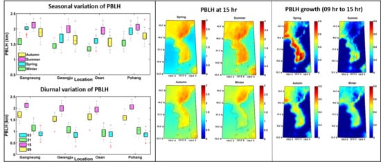
We calculated the PBLH throughout the peninsula at specific times (09:00, 15:00, 21:00, and 03:00 LT). To examine the seasonal variability of the PBLH, we averaged the PBLH seasonally for all years. A box plot with the 5th, 25th, 75th, and 95th percentiles of the average PBLH over each location in each season is shown in Figure 3. This plot shows the mean, maximum, and minimum values of the PBLH at 15:00 LT. It is clearly observed that the PBLH is highest in summer, followed by spring, autumn, and then winter over the Osan (Lat: 37.14, Lon: 127.07), Gwangju (Lat: 35.15, Lon: 126.85), Gangneung (Lat: 37.74, Lon: 128.89), and Pohang (Lat: 36.01, Lon: 129.34) stations. The mean PBLH over Gangneung shows higher values in all four seasons compared to other locations due to the station being located in the mountains. The PBLH is greater than 2 km in summer and less than 1.8 km in winter; while in spring and autumn, it is between 1.5 and 2.1 km. Various atmospheric factors influence the development of the PBL.
The spatial distributions of the mean PBLH throughout the Korean peninsula for all seasons at 09:00, 15:00, 21:00, and 03:00 LT are shown in Figure 4. Figure 4 also clearly shows the seasonal pattern of the PBLH over land. The PBLH reaches its maximum in summer and its minimum in winter. Slightly higher PBLH values tend to occur in spring than in autumn. To describe this PBLH variability in different seasons, we evaluated the controlling factors of the atmosphere. Thus, the seasonal mean values (for each year) of atmospheric surface parameters, such as T, RH, WS, LTS, and Bowen ratio, were estimated. All of these parameters were derived for 09:00, 15:00, 21:00, and 03:00 LT. The spatial distributions of the surface T, RH, WS, LTS, and Bowen ratio are shown in Figures S1–S5 (Supplementary Material), respectively. T and RH were highest in summer and lowest in winter. The strong solar radiation favors intense mixing, and this turbulence causes the PBLH to be high in summer. High RH indicates higher moisture content in the air, which is conducive to strong convection and thus the development of the PBLH. It is interesting to note that the Bowen ratio is low in summer due to the higher number of rainy days, which makes soil moisture high. Further, in summer, the southwesterly hot humid air collides with dry air over the Korean peninsula. As a result, an unstable atmosphere is created at the surface, which induces strong convection. This persistent atmospheric instability leads to the development of the PBLH. Thus, strong insolation caused by solar heating and convection contributed to the high PBLH during this season. Despite the Bowen ratio being high in winter (due to less rain), the low insolation produces a low/negative temperature, leading to shallow PBLH. T and RH are slightly higher (or similar) in autumn than in spring, while the Bowen ratio is lower in autumn than in spring, which is caused by soil moisture. Dry soil content is high in spring compared to autumn. The lifting condensation level (LCL) is high in dry soil because of the strong surface heating causing buoyant lifting of surface air; consequently, the mixing layer becomes deeper. In wet soil (autumn), low surface heating tended to decrease the LCL and form a shallow mixed layer. Furthermore, wet soil has a low surface temperature and high moist static energy, implying a higher convective available potential energy (CAPE) compared to the dry soil. Additionally, the majority of the available energy is converted into latent heat due to the high soil moisture content during wet periods. The latent heat flux dominates the surface fluxes and reduces the surface forcings, which decreases the growth of the PBLH. The high surface latent heat flux, low air temperature, and high CAPE cause weaker solenoidal forcing and produce weaker anabatic flow, resulting in a more stable and shallower PBL in wet periods compared to dry periods. Therefore, soil moisture is a critical parameter that characterizes the PBLH. Furthermore, in dry periods, sensible heat flux is higher, which enhances thermal transportation and mixing, thereby increasing the PBLH, and the opposite is true for wet periods. Thus, the dry soil in spring may develop a slightly higher PBLH than in autumn. Intriguing patterns in the variability of the WS and LTS were also observed (see Figures S3 and S4). The WS, LTS, and pressure (not shown) were lowest in summer and highest in winter. The minimum value of the LTS indicates that the unstable condition of the surface may be due to strong turbulence transport or intense convection, which leads to a high PBLH in summer. Further, the LTS is lower in spring compared to autumn, which may be responsible for higher values of PBLH. It is also observed that WS tends to be higher in spring than in autumn (see Figure S3b). It is interesting to note that the eastern part of Korea is occupied by mountainous terrain (see Figure 1), and especially high-elevation terrain is present in the northeast region. Thus, the PBLH produces the highest values over the northeast compared to the lower elevations due to orographic forcing (detailed description is given in the next section). The east coast area also presents higher PBLH than the west coast area for all seasons due to the high elevation. Furthermore, the sea breezes enter from the west coast area, which influences the eddy diffusivity and produces low PBLH. It is also noteworthy that the east coast area consists of low LTS, while the west coast region experiences high LTS and correspondingly presents high (east coast) and low PBLH (west coast) values.
Figure 4 shows the seasonal variability of the PBLH over land, while it does not exhibit the same seasonal pattern over the ocean. It is interesting to note that during the daytime and nighttime hours, the PBLH over the ocean is high (0.8–2 km) in winter and autumn and low (0–1.5 km) in spring and summer. Figure S3 shows that the wind speed is higher (≥4 ms−1) in winter and autumn than in spring and summer (2–3.5 ms−1). High wind speeds cause intense surface forcing that enhances the PBLH. Furthermore, the LTS (Figure S4) exhibits high values in spring and summer, signifying stable conditions, while low values in autumn and winter indicate instability of the atmosphere. However, in spring and summer, the PBLH values during the daytime (0.5–1.5 km) are higher than during the nighttime (<1 km), which may be induced by solar radiation.
3.2. Diurnal Variation of PBLH
Figure 5a shows the diurnal variability of the mean PBLH over four different locations in the summer season. The PBLH is typically high in the daytime and low in the nighttime. It is known that during the daytime, net surface radiation enhances exchange processes; thus, increases in the PBLH are associated with the CBL. At night, the Earth’s surface is cooled by radiative cooling. Thus, the surface is stable, and the CBL is replaced by a nocturnal boundary layer (NBL). At 09:00 LT, solar radiation increases and creates unstable convective conditions at the surface, producing an increasing trend of the PBLH. It is also notable that in the late afternoon (15:00 LT), the PBLH tends to peak at heights greater than 2 km. Several atmospheric factors may influence the PBLH. The diurnal distributions of the PBLH, T, RH, WS, and LTS over the Korean peninsula at 09:00, 15:00, 21:00, and 03:00 LT are shown in Figure 4 and Figures S1–S4, respectively. Figure 4 also shows similar features of diurnal PBLH through the Korean peninsula. High temperature and low RH values prevail during the daytime. Thus, T and RH may play a crucial role in producing high PBLH values [13]. The surface sensible heat flux is also high during the daytime and low at night (figure not shown), indicating the soil moisture. In all four seasons, PBLH was highest at 15:00 LT and lowest at 03:00 LT.
Figure 5b shows the diurnal and seasonal variation of the PBLH throughout the Korean peninsula. The PBLH is averaged for all the land regions of the Korean peninsula for each hour and season. All the above-mentioned features of the PBLH are clearly visible. The PBLH peaks at ~1.9 km during the late afternoon hours (15 LT) and in summer, while it is lowest at ~0.3 km during the night hours (04 or 05 LT) and in winter.
3.3. Latitudinal Variability of PBLH
It is known that a region with high elevation may produce a high PBLH [21]. The high-elevation mountains in the northeastern region cause significant changes in weather conditions. The spatial distributions of T (Figure S1), RH (Figure S2), WS (Figure S3), LTS (Figure S4), and P (figure not shown) show the weather conditions over the mountainous terrain region. The PBLH pattern at 127.5°E longitude over all latitudes considered and is presented in Figure 6. The patterns of the associated atmospheric parameters (T, RH, P, WS, LTS, surface fluxes, and the ozone mass mixing ratio) are shown in Figure 7. The flux data below 34°N are not reported (see Figure 7) because MERRA2 provides them only for the land regions. Figure 6 illustrates the latitudinal variation in the PBLH with minimum PBLH at low latitudes and maximum PBLH at high latitudes, which reflects the impact of terrain forcing. The pressure is lower at higher altitudes than at lower altitudes, while the wind speeds are higher at higher altitudes. Furthermore, the temperature and LTS decrease from lower to higher latitudes. The presence of complex orography creates upward forcing that, together with convective turbulence, increases the PBLH. Then, pollutants may mix within this increased PBLH. The transport of air pollutants from the CBL to the free atmosphere is due to thermally driven wind flows and is reflected as an elevated aerosol layer [21]. Furthermore, mountain and advective venting are the main mechanisms of pollution transport and turbulence mixing caused by convection [18].
Figure 7 shows that high wind speeds cause unstable (low-LTS) conditions in mountainous terrain areas, and orographic forcing takes place. Thus, pollution transport and air mixing (represented by ozone mixing ratio) are high in mountainous terrain areas. As a result, an aerosol layer and the PBL are formed. Previous studies have also shown that pollutant transport is high over mountainous terrain, and accordingly, an aerosol layer is present at high altitudes [21]. Figure 7 also shows the surface sensible and latent heat fluxes (SFLX and LFLX, respectively). The SFLX and LFLX show increasing and decreasing trends, respectively, from low to high latitudes, indicating soil moisture and supporting growth of the PBLH over high latitudes. During the daytime, the PBLH is high in summer; however, during the nighttime, it is most similar in all seasons. Temperature and wind speed play vital roles in the development of the PBL. Finally, we inferred that the PBL is more positively correlated with the wind speed and more negatively correlated with P and LTS at high altitudes than at low altitudes.
3.4. PBLH Growth Rate
The PBLH increases from the morning (07:00 LT) to late afternoon hours (14:00 or 15:00 LT) due to insolation, and then it gradually decreases during night hours. Usually, the maximum PBLH is reached between 14:00 and 15:00 LT over this region, and we used 15:00 LT data. The difference between the PBLH at 15:00 LT and at 09:00 LT is considered as the growth of the PBLH. Figure 8 shows the spatial distribution of the PBLH growth rate (km/6 h) during different seasons. It can clearly be observed that the PBLH growth is higher in spring than in other seasons. The surface sensible flux (figure not shown) is high in spring, indicating dry air on the surface. High wind speed also occurs during this season (see Figure S3b), which may support surface forcing. Thus, the dry air entrainment and surface forcing favor the mixing layer aloft, which influence/increase the PBLH. The latent flux dominates in the summer and autumn seasons (figure not shown) that diminishes the growth of the PBLH. It is interesting to note that the southern region shows the highest growth of the PBLH due to the high insolation. The solar radiation and its growth are higher over the southern region compared to the northern region, which may produce strong turbulence on the surface, leading to higher PBLH.
Finally, we evaluated the correlations between variations in the PBLH and surface atmospheric factors (T, RH, P, WS, and LTS). Table 1, Table 2, Table 3 and Table 4 present the correlations (R) and standard deviations (SD) of the PBLH and surface parameters for the Osan and Gangneung stations. It can be seen that the PBLH is positively correlated with temperature in all four seasons. PBLH is negatively correlated with RH during both the daytime and nighttime; this indicates that any region with a lower-than-average RH has a higher-than-average PBLH [32]. In the daytime, P is negatively correlated with PBLH, whereas during nighttime, there is no significant relationship between them. The wind speed tends to be positively correlated with PBLH. These correlations indicate that turbulence favors PBLH enhancement. In addition, a high PBLH favors atmospheric dispersion of pollutants. As mentioned above, the stability of the air at the Earth’s surface is influenced by both the temperature and wind speed; thus, the LTS is negatively correlated with the PBLH.
3.5. Climatological Trends of PBLH
This section describes the trends of the PBLH and surface temperature for all years. Figure 9 shows the variability of maximum PBLH during summer from 2008 to 2017 at eight different locations. Figure 9 clearly shows an increasing PBLH trend from 2008 to 2017, which increased nearly 0.2 to 0.8 km in all locations over Korea. Several factors, such as temperature, wind, and soil moisture, control/influence PBLH development. However, here, we presented the variability of T. Figure 10 shows the increasing trend of T from 2008 to 2017, which increased by approximately 1–2 °C. The change in the climate/weather may influence the temperature accordingly with PBLH. It is interesting to note that the Gwangju station located in the southwest shows that the PBLH is mostly stable, which may be due to the sea breezes entering Korea through the southwest region during summer. The southwesterly winds may diminish the development of the PBLH. The Osan and Paju (Lat: 37.7, Lon: 126.7) stations (located on the west side) also showed a diminished increase in the PBLH, which caused the southwesterly winds to influence its increment. However, the Wonju and Daegu stations are in the middle region (not coastal areas) of South Korea; thus, westerly winds may have less effect on PBLH. Furthermore, the surface temperature was also high at these stations (especially Daegu) (see Figure 10 and Figure S1). Therefore, the PBLH was enhanced in the central part of Korea. On the other hand, the Gangneung and Pohang stations are located at the east side and occupied by mountainous terrain, and the Toksong station (Lat: 40.3, Lon: 128.2) is in the high-terrain region located in the northeast region of the Korean peninsula (see Figure 1). The strong winds present over these mountainous locations (see Figure S3) produce strong turbulence, and terrain forcing may increase the PBLH. Further, Figure 10 shows that T also increased from 2007 to 2018. The distributions of PBLH and T over these eight geographical stations are shown in Figure 11, and their statistics are presented in Table 5. It can be clearly observed that the Daegu and Wonju stations show high PBLH and T. However, Osan shows low PBLH and T. Wind and other parameters also influence the PBLH (sea breezes affect the east side and strong winds over mountainous terrain); however, PBLH and T showed mostly similar distributions. Table 5 shows the quantile 95 (Q95) values of PBLH and T as well as Spearman’s correlation between the two. The Osan, Gwangju, Toksong, and Gangneung stations were influenced by wind speed, thus showing low Spearman’s correlations. Finally, from Figure 9 and Figure 10, we inferred that the climate changed from 2007 to 2018 over the Korean peninsula.
4. Summary and Conclusions
This paper presented the climatology of the PBLH over the Korean peninsula for the period from 2008 to 2017. We estimated the PBLH using the bulk Richardson number method with a critical value of 0.25. This method is effective for both stable and convective boundary layers. The PBLH values derived from ERA5 data were validated using radiosonde and GPSRO measurements. The PBLH is highest in summer, followed by spring, autumn, and then winter (similar to Lee et al., 2011). Strong solar radiation in summer favors turbulence mixing and PBLH enhancement. The Bowen ratio is high (low soil moisture) in spring compared to autumn, which leads to a slightly higher PBLH in spring. The low/negative temperature (low insolation) is responsible for the low PBLH in winter. During the daytime, the PBLH increases with increasing solar radiation, peaking in the late afternoon (around 15:00 LT). During the nighttime, the PBLH decreases because of radiative cooling. Over the high-elevation region, high wind speeds enhance wind shearing and upward forcing, which generates turbulence and increases the PBLH. Furthermore, the low pressure allows strong airflow over the mountains, thus producing a low LTS. The mountainous region had high PBLH owing to orographic lifting and strong convection. The PBLH over land in plain areas is mostly positively correlated with T and WS and negatively correlated with RH, LTS, and P. The growth rate of the PBLH is high in spring because of the low soil moisture indicated by the high SFLX. Southern regions have strong solar insolation growth, leading to large growth of the PBL. The PBLH seasonal patterns do not persist over the oceans. Over the ocean regions, the PBLH is greater during winter and autumn owing to high wind speeds, while the opposite is true in spring and summer. We also observed that the PBLH increased from 2008 to 2017 over the Korean peninsula. Further, an increasing trend of T was also observed from 2008 to 2017. Thus, we inferred that the temperature and PBLH increased due to changing of the climate in the last decade over this region.
The climatology of the PBLH over the Korean peninsula described in this paper can be useful for better understanding the formation of convection, clouds, and extreme precipitation due to rainfall and snowfall. In the future, the merits and demerits associated with PBLH estimations can be studied based on wind profiling radar and radiosonde networks over this region. Further, a comprehensive investigation of the PBLH-associated aerosol layer structure over urban areas during air pollution episodes will be conducted. The PBLH change/enhancement due to climate change over 40 years will also be studied.
Supplementary Materials
The following are available online at https://www.mdpi.com/2072-4292/12/16/2571/s1, Figure S1: Spatial distribution of average surface temperature from 2008 to 2017: (a) 09:00 LT, (b) 15:00 LT, (c) 21:00 LT, and (d) 03:00 LT, Figure S2: Spatial distribution of average surface relative humidity from 2008 to 2017: (a) 09:00 LT, (b) 15:00 LT, (c) 21:00 LT, and (d) 03:00 LT, Figure S3: Spatial distribution of average 10-m wind speed from 2008 to 2017: (a) 09:00 LT, (b) 15:00 LT, (c) 21:00 LT, and (d) 03:00 LT, Figure S4: Spatial distribution of average LTS from 2008 to 2017: (a) 09:00 LT, (b) 15:00 LT, (c) 21:00 LT, and (d) 03:00 LT, Figure S5: Spatial distribution of average Bowen ratio from 2008 to 2017: (a) 09:00 LT, (b) 15:00 LT, (c) 21:00 LT, and (d) 03:00 LT.
Author Contributions
S.A. performed data analyses and conceptualization and wrote the first manuscript draft. S.L. provided helpful discussions on the analyses of data, conceptualization, methodology, and review and edited the manuscript. All authors have read and agreed to the published version of the manuscript.
Funding
This work was supported by the Korea Institute of Civil Engineering and Building Technology Strategic Research Project (Establishment of 3D Fine Dust Information Based on AI Image Analysis).
Acknowledgments
This work was supported by the Korea Institute of Civil Engineering and Building Technology Strategic Research Project (Establishment of 3D Fine Dust Information Based on AI Image Analysis). The authors would like to thank the ECMWF and the University of Wyoming for providing the datasets used in this study.
Conflicts of Interest
The authors declare no conflicts of interest.
References
- Stull, R.B. An Introduction to Boundary Layer Meteorology; Kluwer Academic Publishers: Norwell, MA, USA, 1988; p. 666. [Google Scholar]
- Garratt, J.R. The atmospheric boundary layer. In Cambridge Atmospheric and Space Science Series; Cambridge University Press: Cambridge, UK, 1992; Volume 416, p. 444. [Google Scholar]
- White, A.B.; Fairall, C.W.; Wolfe, D.E. Use of 915 MHz wind profiler data to describe the diurnal variability of the mixed layer. In Proceedings of the 7th Symposium on Meteorological Observations and Instrumentations, New Orleans, LA, USA, 14–18 January 1991; pp. J161–J166. [Google Scholar]
- Allabakash, S.; Yasodha, P.; Bianco, L.; Venkatramana Reddy, S.; Srinivasulu, P.; Lim, S. Improved boundary layer height measurement using a fuzzy logic method: Diurnal and seasonal variabilities of the convective boundary layer over a tropical station. J. Geophys. Res. Atmos. 2017, 122, 9211–9232. [Google Scholar] [CrossRef]
- Basha, G.; Ratnam, M.V. Identification of atmospheric boundary layer height over a tropical station using high-resolution radiosonde refractivity profiles: Comparison with GPS radio occultation measurements. J. Geophys. Res. Atmos. 2009, 114, D16101. [Google Scholar] [CrossRef]
- Bianco, L.; Djalalova, I.V.; King, C.W.; Wilczak, J.M. Diurnal evolution and annual variability of boundary-layer height and its correlation to other meteorological variables in California’s Central Valley. Bound. Layer Meteorol. 2011, 140, 491–511. [Google Scholar] [CrossRef] [Green Version]
- Emeis, S.; Münkel, C.; Vogt, S.; Müller, W.J.; Schäfer, K. Atmospheric boundary-layer structure from simultaneous SODAR, RASS, and ceilometer measurements. Atmos. Environ. 2004, 38, 273–286. [Google Scholar] [CrossRef]
- Coulter, R.L. A comparison of three methods for measuring mixing-layer height. J. Appl. Meteorol. 1979, 18, 1495–1499. [Google Scholar] [CrossRef] [Green Version]
- Seibert, P.; Beyrich, F.; Gryning, S.E.; Joffre, S.; Rasmussen, A.; Tercier, P. Review and intercomparison of operational methods for the determination of the mixing height. Dev. Environ. Sci. 2002, 1, 569–613. [Google Scholar] [CrossRef]
- Cornman, L.B.; Goodrich, R.K.; Morse, C.S.; Ecklund, W.L. A fuzzy logic method for improved moment estimation from Doppler spectra. J. Atmos. Ocean. Technol. 1998, 15, 1287–1305. [Google Scholar] [CrossRef] [Green Version]
- Ao, Y.; Li, J.; Li, Z.; Lyu, S.; Jiang, C.; Wang, M. Relation between the atmospheric boundary layer and impact factors under severe surface thermal conditions. Adv. Meteorol. 2017, 2017, 1–12. [Google Scholar] [CrossRef]
- Basha, G.; Kishore, P.; Ratnam, M.V.; Babu, S.R.; Velicogna, I.; Jiang, J.H.; Ao, C.O. Global climatology of planetary boundary layer top obtained from multi-satellite GPS RO observations. Clim. Dyn. 2019, 52, 2385–2398. [Google Scholar] [CrossRef]
- Seidel, D.J.; Ao, C.O.; Li, K. Estimating climatological planetary boundary layer heights from radiosonde observations: Comparison of methods and uncertainty analysis. J. Geophys. Res. Atmos. 2010, 115, D16113. [Google Scholar] [CrossRef] [Green Version]
- Seidel, D.J.; Zhang, Y.; Beljaars, A.; Golaz, J.C.; Jacobson, A.R.; Medeiros, B. Climatology of the planetary boundary layer over the continental United States and Europe. J. Geophys. Res. Atmos. 2012, 117, D17106. [Google Scholar] [CrossRef]
- von Engeln, A.; Teixeira, J. A planetary boundary layer height climatology derived from ECMWF reanalysis data. J. Clim. 2013, 26, 6575–6590. [Google Scholar] [CrossRef]
- Guo, J.; Miao, Y.; Zhang, Y.; Liu, H.; Li, Z.; Zhang, W.; He, J.; Lou, M.; Yan, Y.; Bian, L.; et al. The climatology of planetary boundary layer height in China derived from radiosonde and reanalysis data. Atmos. Chem. Phys. 2016, 16, 13309–13319. [Google Scholar] [CrossRef] [Green Version]
- Guo, P.; Kuo, Y.H.; Sokolovskiy, S.V.; Lenschow, D.H. Estimating atmospheric boundary layer depth using COSMIC radio occultation data. J. Atmos. Sci. 2011, 68, 1703–1713. [Google Scholar] [CrossRef]
- De Wekker, S.F.J.; Kossmann, M.; Fielder, F. Observations of daytime mixed layer heights over mountainous terrain during the TRACT field campaign. In Proceedings of the 12th American Meteorological Society Symposium on Boundary Layers and Turbulence, Vancouver, BC, Canada, 28 July–1 August 1997; pp. 498–499. [Google Scholar]
- Lieman, R.; Alpert, P. Investigation of the planetary boundary layer height variations over complex terrain. Bound. Layer Meteorol. 1993, 62, 129–142. [Google Scholar] [CrossRef]
- Kalthoff, N.; Binder, H.J.; Kossmann, M.; Vögtlin, R.; Corsmeier, U.; Fiedler, F.; Schlager, H. Temporal evolution and spatial variation of the boundary layer over complex terrain. Atmos. Environ. 1998, 32, 1179–1194. [Google Scholar] [CrossRef]
- De Wekker, S.F.; Kossmann, M. Convective boundary layer heights over mountainous terrain—A review of concepts. Front. Earth Sci. 2015, 3, 77. [Google Scholar] [CrossRef] [Green Version]
- Choi, J.S.; Baek, S.O. An approach to estimate daily maximum mixing height (DMMH) in Pohang, Osan, and Kwangju areas—Analysis of 10 years data from 1983 to 1992. J. Korea Air Pollut. Res. Assoc. 1998, 14, 379–385. [Google Scholar]
- Yoon, S.C.; Won, J.G.; Kim, S.W.; Lim, G.M. Measurement of Mixed Layer Height Using Lidar. Proceedings of the Korean Society for Atmospheric Environment. 1999, pp. 436–437. Available online: https://scholar.google.com/scholar_lookup?title=Measurement%20of%20mixed%20layer%20height%20using%20Lidar&author=S.-C.%20Yoon&author=J.-G.%20Won&author=S.-W.%20Kim&author=&author=G.-M.%20Lim&publication_year=1999 (accessed on 8 August 2020).
- Lee, S.J.; Kawai, H. Mixing depth estimation from operational JMA and KMA wind-profiler data and its preliminary applications: Examples from four selected sites. J. Meteorol. Soc. Jpn. Ser. II 2011, 89, 15–28. [Google Scholar] [CrossRef] [Green Version]
- Lee, S.J.; Kim, J.; Cho, C.H. An automated monitoring of atmospheric mixing height from routine radiosonde profiles over South Korea using a web-based data transfer method. Environ. Monitor. Assess. 2014, 186, 3253–3263. [Google Scholar] [CrossRef]
- Lee, S.J.; Lee, J.; Greybush, S.J.; Kang, M.; Kim, J. Spatial and temporal variation in PBL height over the Korean Peninsula in the KMA operational regional model. Adv. Meteorol. 2013, 2013, 1–16. [Google Scholar] [CrossRef]
- Hersbach, H.; Dee, D. ERA5 reanalysis is in production. ECMWF Newslett. 2016, 147, 7. [Google Scholar]
- Slingo, J.M. The development and verification of a cloud prediction scheme for the ECMWF model. Q. J. R. Meteorol. Soc. 1987, 113, 899–927. [Google Scholar] [CrossRef]
- Sokolovskiy, S.; Kuo, Y.H.; Rocken, C.; Schreiner, W.S.; Hunt, D.; Anthes, R.A. Monitoring the atmospheric boundary layer by GPS radio occultation signals recorded in the open-loop mode. Geophys. Res. Lett. 2006, 33, L12813. [Google Scholar] [CrossRef] [Green Version]
- Davy, R. The climatology of the atmospheric boundary layer in contemporary global climate models. J. Clim. 2018, 31, 9151–9173. [Google Scholar] [CrossRef]
- Vogelezang, D.H.P.; Holtslag, A.A.M. Evaluation and model impacts of alternative boundary-layer height formulations. Bound. Layer Meteorol. 1996, 81, 245–269. [Google Scholar] [CrossRef]
- Zhang, Y.; Seidel, D.J.; Zhang, S. Trends in planetary boundary layer height over Europe. J. Clim. 2013, 26, 10071–10076. [Google Scholar] [CrossRef]
Figure 1.
Topography of the Korean peninsula.
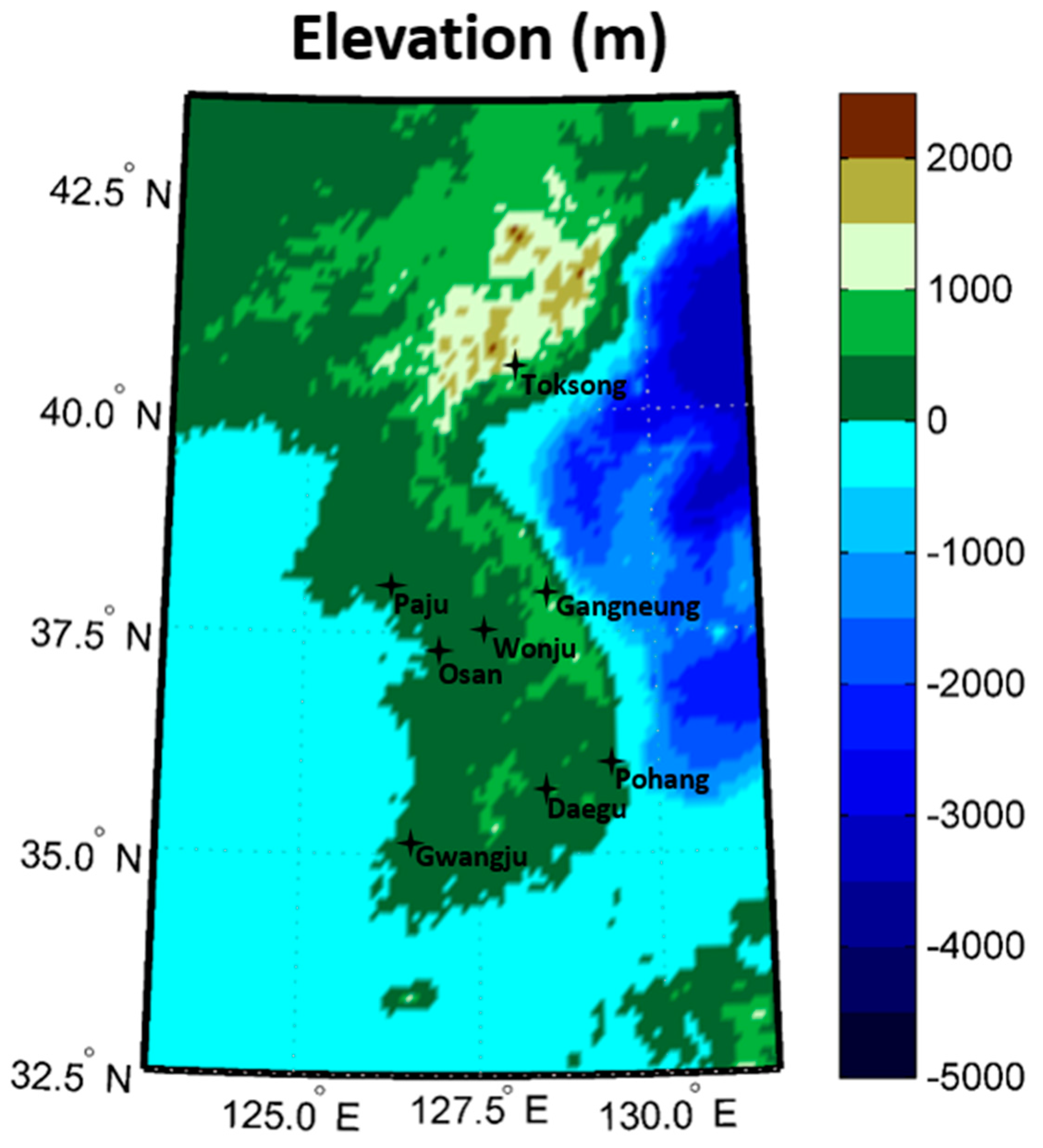
Figure 2.
(a) Scatter plots of planetary boundary layer height (PBLH) derived from ERA5 and sounding datasets over four different geographical locations (Osan, Gwangju, Gangneung, and Pohang). (b) PBLH derived from ERA5 and global positioning system radio occultation (GPSRO) for the year 2008.
Figure 2.
(a) Scatter plots of planetary boundary layer height (PBLH) derived from ERA5 and sounding datasets over four different geographical locations (Osan, Gwangju, Gangneung, and Pohang). (b) PBLH derived from ERA5 and global positioning system radio occultation (GPSRO) for the year 2008.
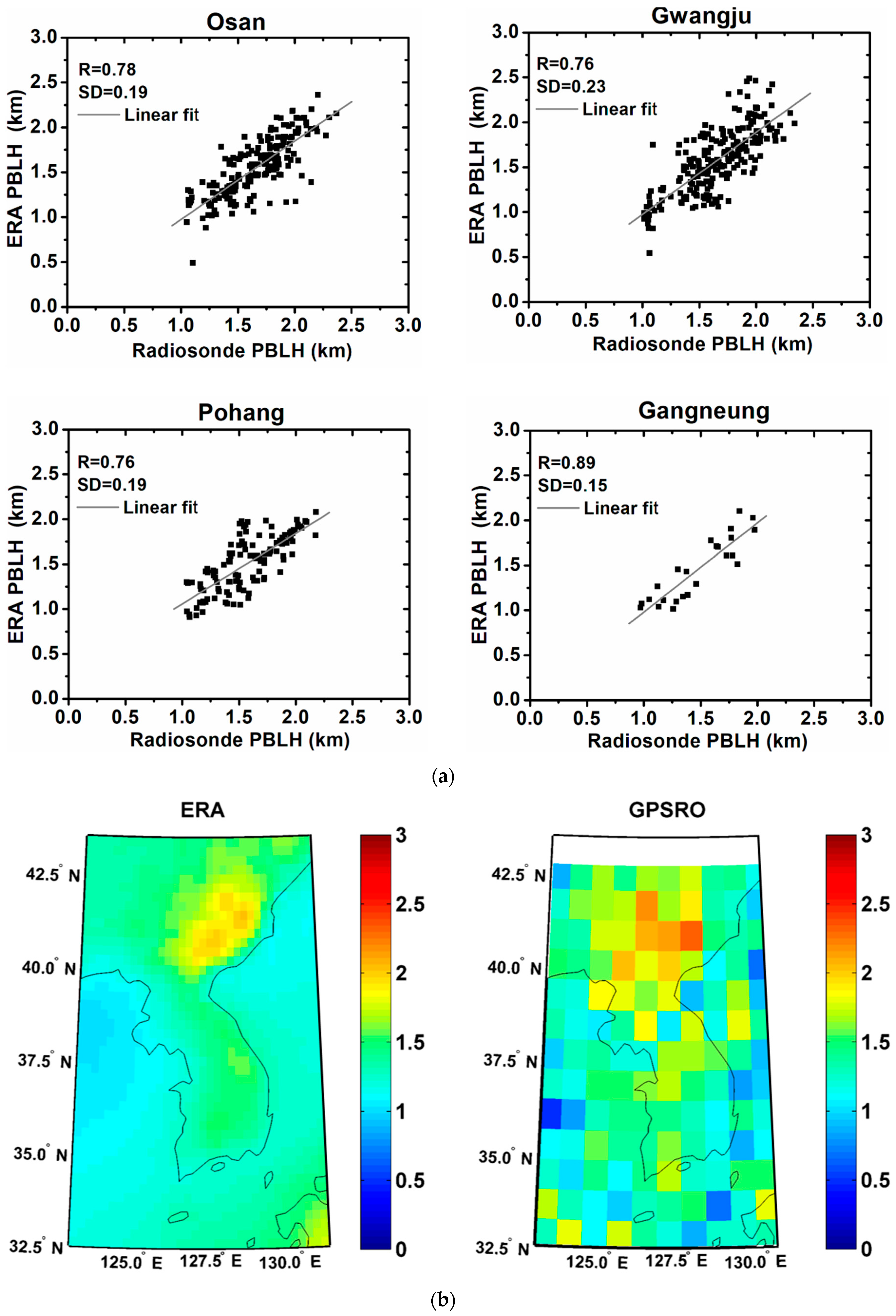
Figure 3.
Box plot of the 5th, 25th, 75th, and 95th percentiles of the average PBLH in each season for 10 years (2008–2017) over Osan, Gwangju, Gangneung, and Pohang stations.
Figure 3.
Box plot of the 5th, 25th, 75th, and 95th percentiles of the average PBLH in each season for 10 years (2008–2017) over Osan, Gwangju, Gangneung, and Pohang stations.
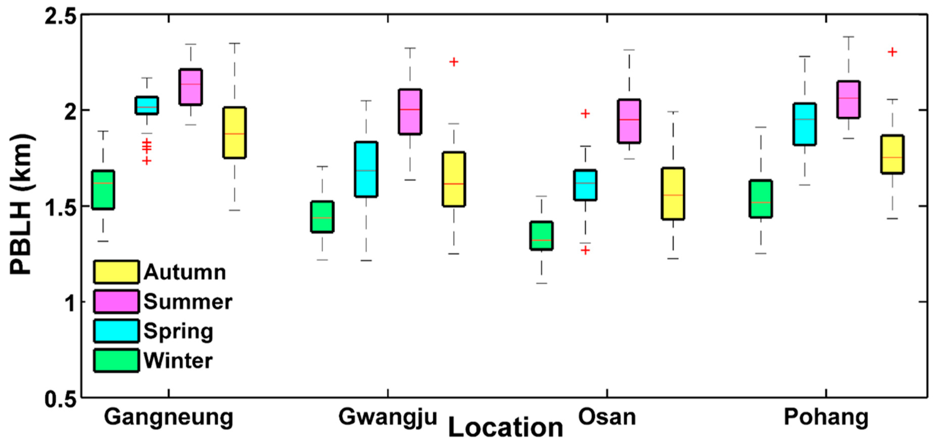
Figure 4.
Spatial distribution of average PBLH from 2008 to 2017: (a) 09:00 LT, (b) 15:00 LT, (c) 21:00 LT, and (d) 03:00 LT.
Figure 4.
Spatial distribution of average PBLH from 2008 to 2017: (a) 09:00 LT, (b) 15:00 LT, (c) 21:00 LT, and (d) 03:00 LT.

Figure 5.
(a) Diurnal variability of the average PBLH (2008–2017) in summer for the Osan, Gwangju, Gangneung, and Pohang stations. (b) Diurnal and seasonal variation of the mean PBLH throughout Korean peninsula.
Figure 5.
(a) Diurnal variability of the average PBLH (2008–2017) in summer for the Osan, Gwangju, Gangneung, and Pohang stations. (b) Diurnal and seasonal variation of the mean PBLH throughout Korean peninsula.

Figure 6.
Latitudinal variation of average PBLH at 127.5°E longitude from 2008 to 2017 at 09:00, 15:00, 21:00, and 03:00 LT (local time).
Figure 6.
Latitudinal variation of average PBLH at 127.5°E longitude from 2008 to 2017 at 09:00, 15:00, 21:00, and 03:00 LT (local time).

Figure 7.
(a) Latitudinal variation of average surface temperature, relative humidity, pressure, and wind speed at 127.5°E longitude from 2008 to 2017 at 09:00, 15:00, 21:00, and 03:00 LT. (b) Latitudinal variation of average surface LTS, ozone mixing ratio, surface sensible heat flux (SFLX), and latent heat flux (LFLX) at 127.5°E longitude. However, the fluxes over land and at 09:30, 15:30, 21:30, and 03:30 LT.
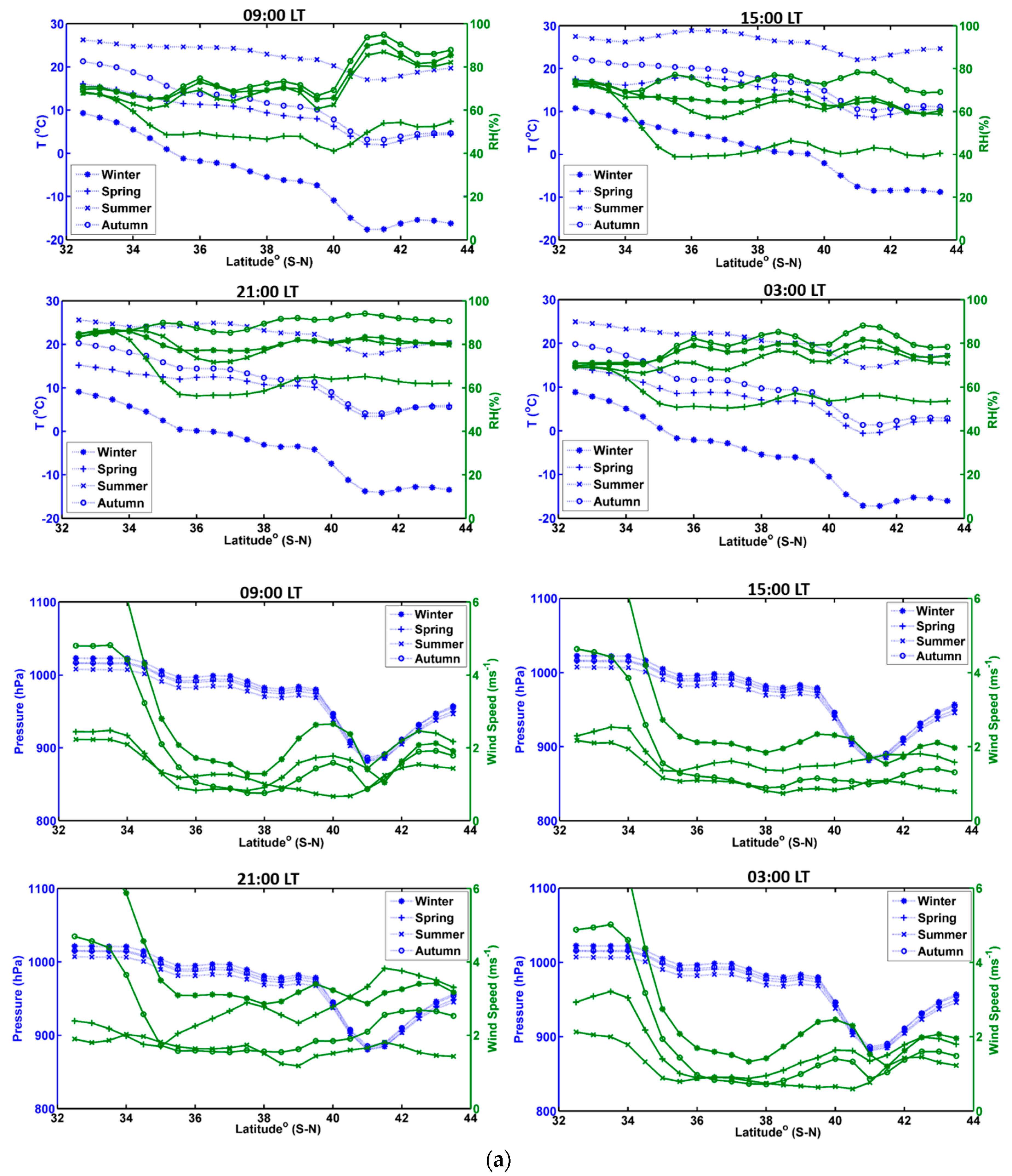

Figure 8.
Spatial distribution of average PBLH growth rate from 09:00 LT to 15:00 LT (km/6 h).

Figure 9.
Variability of the maximum PBLH during summer from 2008 to 2017. The error bars and dashed red lines indicate the standard deviation and linear fit of the data, respectively.
Figure 9.
Variability of the maximum PBLH during summer from 2008 to 2017. The error bars and dashed red lines indicate the standard deviation and linear fit of the data, respectively.
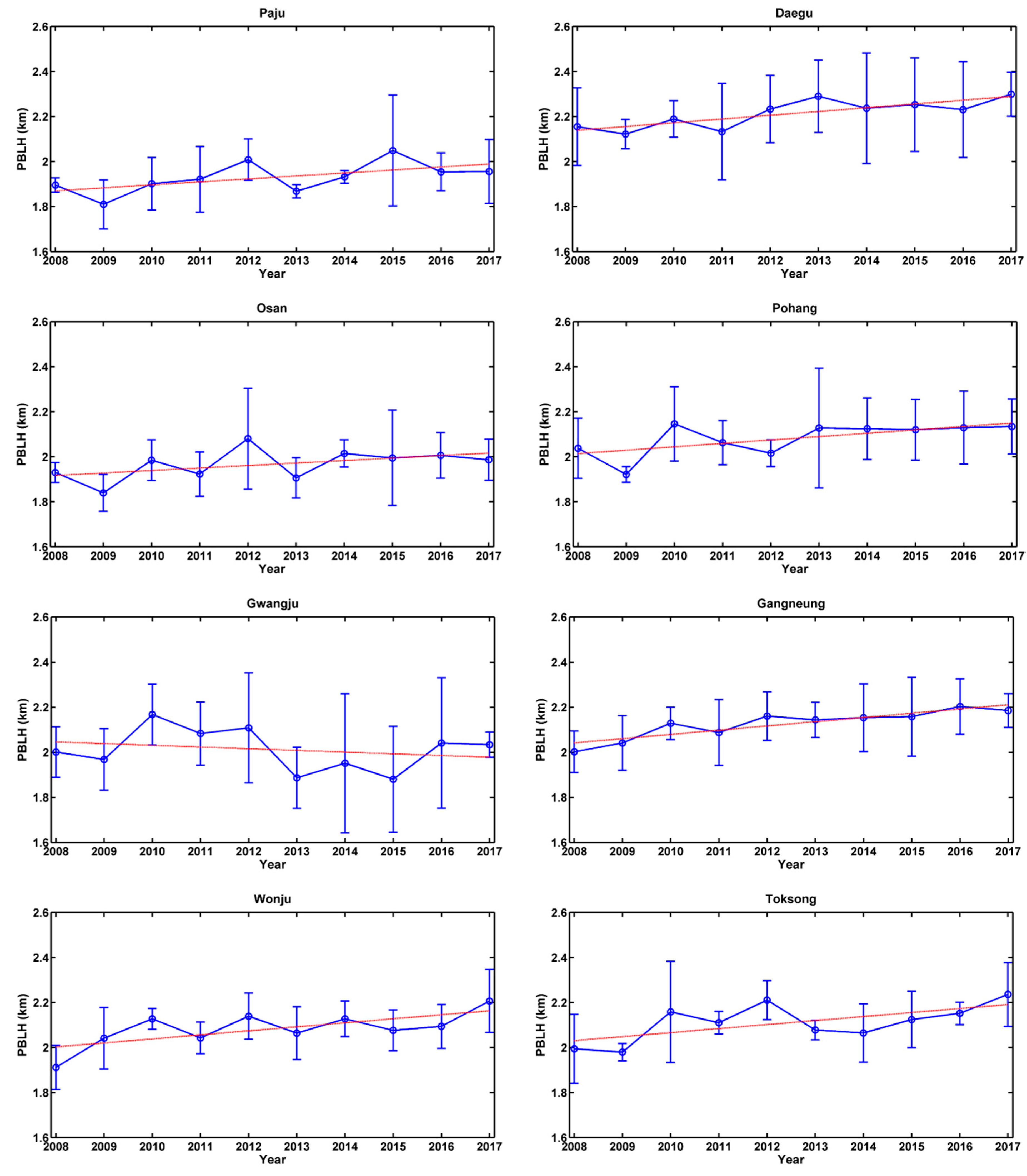
Figure 10.
Variability of the maximum surface temperature during summer from 2008 to 2017. The error bars and dashed red lines indicate the standard deviation and linear fit of the data, respectively.
Figure 10.
Variability of the maximum surface temperature during summer from 2008 to 2017. The error bars and dashed red lines indicate the standard deviation and linear fit of the data, respectively.

Figure 11.
Distributions of PBLH and temperature (T) over different geographical stations.


Table 1.
Correlations between PBLH and meteorological parameters during winter.
| Station | Winter (Daytime) | Winter (Nighttime) | ||||||||||||||||||
|---|---|---|---|---|---|---|---|---|---|---|---|---|---|---|---|---|---|---|---|---|
| T | RH | P | WS | LTS | T | RH | P | WS | LTS | |||||||||||
| R | SD | R | SD | R | SD | R | SD | R | SD | R | SD | R | SD | R | SD | R | SD | R | SD | |
| Osan | 0.3 | 3.4 | −0.5 | 7.5 | −0.07 | 214 | 0.5 | 0.82 | −0.5 | 2.1 | 0.07 | 2.3 | −0.4 | 4.3 | 0.1 | 195 | 0.4 | 0.4 | −0.3 | 2.0 |
| Gangneung | 0.6 | 2.6 | −0.6 | 7.9 | −0.4 | 198 | 0.03 | 0.9 | −0.6 | 1.8 | 0.2 | 2.2 | −0.2 | 6.7 | 0.2 | 180 | −0.2 | 0.7 | −0.4 | 1.6 |
Table 2.
Correlations between PBLH and meteorological parameters during spring.
| Station | Spring (Daytime) | Spring (Nighttime) | ||||||||||||||||||
|---|---|---|---|---|---|---|---|---|---|---|---|---|---|---|---|---|---|---|---|---|
| T | RH | P | WS | LTS | T | RH | P | WS | LTS | |||||||||||
| R | SD | R | SD | R | SD | R | SD | R | SD | R | SD | R | SD | R | SD | R | SD | R | SD | |
| Osan | 0.5 | 5.5 | −0.7 | 0.5 | −0.3 | 348 | 0.7 | 0.8 | −0.7 | 2.0 | −0.1 | 5.1 | −0.1 | 6.6 | 0.1 | 362 | 0.2 | 0.6 | 0.2 | 1.9 |
| Gangneung | 0.3 | 5.7 | −0.6 | 9.0 | −0.2 | 300 | −0.07 | 0.7 | −0.6 | 2.14 | −0.4 | 4.7 | −0.3 | 6.1 | 0.3 | 287 | 0.1 | 0.6 | −0.1 | 2.3 |
Table 3.
Correlations between PBLH and meteorological parameters during summer.
| Station | Summer (Daytime) | Summer (Nighttime) | ||||||||||||||||||
|---|---|---|---|---|---|---|---|---|---|---|---|---|---|---|---|---|---|---|---|---|
| T | RH | P | WS | LTS | T | RH | P | WS | LTS | |||||||||||
| R | SD | R | SD | R | SD | R | SD | R | SD | R | SD | R | SD | R | SD | R | SD | R | SD | |
| Osan | 0.4 | 2.3 | −0.1 | 13 | −0.2 | 140 | 0.3 | 0.9 | −0.05 | 2.2 | 0.6 | 1.7 | −0.03 | 8.1 | −0.04 | 119 | 0.1 | 0.6 | −0.1 | 1.6 |
| Gangneung | 0.6 | 1.8 | −0.2 | 9.8 | −0.1 | 152 | 0.1 | 0.8 | −0.2 | 1.8 | 0.6 | 1.8 | −0.09 | 5.8 | −0.07 | 143 | 0.09 | 0.6 | 0.01 | 1.8 |
Table 4.
Correlations between PBLH and meteorological parameters during autumn.
| Station | Autumn (Daytime) | Autumn (Nighttime) | ||||||||||||||||||
|---|---|---|---|---|---|---|---|---|---|---|---|---|---|---|---|---|---|---|---|---|
| T | RH | P | WS | LTS | T | RH | P | WS | LTS | |||||||||||
| R | SD | R | SD | R | SD | R | SD | R | SD | R | SD | R | SD | R | SD | R | SD | R | SD | |
| Osan | 0.4 | 5.9 | −0.3 | 10 | −0.3 | 341 | 0.2 | 0.7 | −0.6 | 2.3 | 0.2 | 5.5 | −0.2 | 5.6 | −0.1 | 346 | 0.1 | 0.4 | −0.2 | 1.9 |
| Gangneung | 0.5 | 4.9 | −0.2 | 11 | −0.4 | 260 | −0.2 | 1.03 | −0.4 | 1.8 | 0.03 | 5.4 | −0.2 | 7.1 | 0.2 | 261 | −0.04 | 0.8 | −0.08 | 1.5 |
Table 5.
Q95 and Spearman correlations of PBLH and T.
| Station | Q95 | Spearman’s Correlation | |
|---|---|---|---|
| PBLH (km) | T (°C) | ||
| Paju | 2.0 | 31.1 | 0.84 |
| Osan | 2.0 | 29.9 | 0.51 |
| Gwangju | 2.1 | 29.7 | −0.23 |
| Wonju | 2.2 | 31.1 | 0.76 |
| Daegu | 2.2 | 31.9 | 0.78 |
| Pohang | 2.1 | 32.3 | 0.66 |
| Gangneung | 2.1 | 31.5 | 0.16 |
| Toksong | 2.2 | 30.4 | −0.13 |
© 2020 by the authors. Licensee MDPI, Basel, Switzerland. This article is an open access article distributed under the terms and conditions of the Creative Commons Attribution (CC BY) license (http://creativecommons.org/licenses/by/4.0/).
Share and Cite
MDPI and ACS Style
Allabakash, S.; Lim, S. Climatology of Planetary Boundary Layer Height-Controlling Meteorological Parameters Over the Korean Peninsula. Remote Sens. 2020, 12, 2571. https://doi.org/10.3390/rs12162571
AMA Style
Allabakash S, Lim S. Climatology of Planetary Boundary Layer Height-Controlling Meteorological Parameters Over the Korean Peninsula. Remote Sensing. 2020; 12(16):2571. https://doi.org/10.3390/rs12162571
Chicago/Turabian StyleAllabakash, Shaik, and Sanghun Lim. 2020. "Climatology of Planetary Boundary Layer Height-Controlling Meteorological Parameters Over the Korean Peninsula" Remote Sensing 12, no. 16: 2571. https://doi.org/10.3390/rs12162571
Note that from the first issue of 2016, this journal uses article numbers instead of page numbers. See further details here.