A New Modeling Approach for Spatial Prediction of Flash Flood with Biogeography Optimized CHAID Tree Ensemble and Remote Sensing Data

 , ,
, ,  , , , and
Abstract
:
1. Introduction
2. Study Area and Data
2.1. Study Area
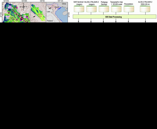
2.2. Data
2.2.1. Land-Use/Land-Cover (LULC)
2.2.2. Soil Type
2.2.3. Lithology
3. The Employed Methods
3.1. Chi-Square Automatic Interaction Detection (CHAID)
3.2. Random Subspace Ensemble (RSE)
3.3. Biogeography-Based Optimization (BBO)
4. Proposed CHAID-RS-BBO Model for Flash Flood Susceptibility Modeling
4.1. Flash-Flood Database Establishment, Coding and Checking
4.2. Establishing the CHAID-RS and the Cost Function
4.3. Optimizing the CHAID-RS Using the BBO Algorithm
4.4. Final CHAID-RS-BBO Model and Flash Flood Susceptibility
5. Results
5.1. Correlation of the Predictors of Flash Floods
5.2. Training the Flash Flood Models
5.3. Validating the Fflash Flood Models
5.4. Flash Flood Susceptibility Maps
6. Discussion
7. Concluding Remarks
- ▪
- With the flash flood inventories and six predictors, the remote sensing data, Sentinel-1 SAR, Sentinel-2 and ALOS–PALSAR DEM, are important sources for flash flood modeling.
- ▪
- With its high performance, it can be concluded that CHAID-RS-BBO is a new tool for flash flood modeling.
- ▪
- The susceptibility map, which reveals the flash flood hotspots in Luc Yen, might help the local government and decision-makers to minimize the flash flood impacts in the selection and collection of the water of the flash floods for life requirements and development projects.
- ▪
- The current study recommends the creation of precise and updated meteorology, morphometry, hydrology, geology, topography, and socioeconomic studies. Early warning systems (EWS) have to be developed to predict flash floods and consequently minimize losses and reduce damage. Last, but not least, a national plan for flash-flood disaster management and risk reduction has to be enabled.
Author Contributions
Funding
Conflicts of Interest
References
- Fernandes, O.; Murphy, R.; Adams, J.; Merrick, D. Quantitative Data Analysis: CRASAR Small Unmanned Aerial Systems at Hurricane Harvey. In Proceedings of the 2018 IEEE International Symposium on Safety, Security, and Rescue Robotics (SSRR), Philadelphia, PA, USA, 6–8 August 2018. [Google Scholar]
- Marchi, L.; Borga, M.; Preciso, E.; Gaume, E. Characterisation of selected extreme flash floods in Europe and implications for flood risk management. J. Hydrol. 2010, 394, 118–133. [Google Scholar] [CrossRef]
- Kjeldsen, T.R. Modelling the impact of urbanization on flood frequency relationships in the UK. Hydrol. Res. 2010, 41, 391–405. [Google Scholar] [CrossRef] [Green Version]
- Alexander, L.V. Global observed long-term changes in temperature and precipitation extremes: A review of progress and limitations in IPCC assessments and beyond. Weather Clim. Extrem. 2016, 11, 4–16. [Google Scholar] [CrossRef] [Green Version]
- Shafapour Tehrany, M.; Kumar, L.; Shabani, F. A novel GIS-based ensemble technique for flood susceptibility mapping using evidential belief function and support vector machine: Brisbane, Australia. PeerJ 2019, 7, e7653. [Google Scholar] [CrossRef]
- Lyu, H.M.; Sun, W.J.; Shen, S.L.; Arulrajah, A. Flood risk assessment in metro systems of mega-cities using a GIS-based modeling approach. Sci. Total Environ. 2018, 626, 1012–1025. [Google Scholar] [CrossRef]
- Yu, J.J.; Qin, X.S.; Larsen, O. Joint Monte Carlo and possibilistic simulation for flood damage assessment. Stoch. Environ. Res. Risk Assess. 2012, 27, 725–735. [Google Scholar] [CrossRef]
- Merz, B.; Kreibich, H.; Schwarze, R.; Thieken, A. Review article “Assessment of economic flood damage”. Nat. Hazards Earth Syst. Sci. 2010, 10, 1697–1724. [Google Scholar] [CrossRef]
- Ogie, R.I.; Adam, C.; Perez, P. A review of structural approach to flood management in coastal megacities of developing nations: Current research and future directions. J. Environ. Plan. Manag. 2019, 63, 127–147. [Google Scholar] [CrossRef]
- Gourley, J.J.; Flamig, Z.L.; Vergara, H.; Kirstetter, P.E.; Clark, R.A.; Argyle, E.; Arthur, A.; Martinaitis, S.; Terti, G.; Erlingis, J.M.; et al. The FLASH Project: Improving the Tools for Flash Flood Monitoring and Prediction across the United States. Bull. Am. Meteorol. Soc. 2017, 98, 361–372. [Google Scholar] [CrossRef]
- Archer, D.R.; Fowler, H.J. Characterising flash flood response to intense rainfall and impacts using historical information and gauged data in Britain. J. Flood Risk Manag. 2015, 11, S121–S133. [Google Scholar] [CrossRef]
- Chang, H.; Franczyk, J. Climate change, land-use change, and floods: Toward an integrated assessment. Geogr. Compass 2008, 2, 1549–1579. [Google Scholar] [CrossRef]
- Rahmati, O.; Darabi, H.; Haghighi, A.T.; Stefanidis, S.; Kornejady, A.; Nalivan, O.A.; Tien Bui, D. Urban Flood Hazard Modeling Using Self-Organizing Map Neural Network. Water 2019, 11, 2370. [Google Scholar] [CrossRef] [Green Version]
- Mansur, A.V.; Brondizio, E.S.; Roy, S.; de Miranda Araújo Soares, P.P.; Newton, A. Adapting to urban challenges in the Amazon: Flood risk and infrastructure deficiencies in Belém, Brazil. Reg. Environ. Chang. 2017, 18, 1411–1426. [Google Scholar] [CrossRef]
- Zhou, Z.; Liu, S.; Zhong, G.; Cai, Y. Flood Disaster and Flood Control Measurements in Shanghai. Nat. Hazards Rev. 2017, 18. [Google Scholar] [CrossRef]
- Papaioannou, G.; Efstratiadis, A.; Vasiliades, L.; Loukas, A.; Papalexiou, S.; Koukouvinos, A.; Tsoukalas, I.; Kossieris, P. An Operational Method for Flood Directive Implementation in Ungauged Urban Areas. Hydrology 2018, 5, 24. [Google Scholar] [CrossRef] [Green Version]
- Barredo, J.I.; Engelen, G. Land Use Scenario Modeling for Flood Risk Mitigation. Sustainability 2010, 2, 1327–1344. [Google Scholar] [CrossRef] [Green Version]
- Winsemius, H.C.; Van Beek, L.P.H.; Jongman, B.; Ward, P.J.; Bouwman, A. A framework for global river flood risk assessments. Hydrol. Earth Syst. Sci. 2013, 17, 1871–1892. [Google Scholar] [CrossRef] [Green Version]
- Tsakiris, G. Flood risk assessment: Concepts, modelling, applications. Nat. Hazards Earth Syst. Sci. 2014, 14, 1361–1369. [Google Scholar] [CrossRef] [Green Version]
- Tien Bui, D.; Pradhan, B.; Nampak, H.; Bui, Q.T.; Tran, Q.A.; Nguyen, Q.P. Hybrid artificial intelligence approach based on neural fuzzy inference model and metaheuristic optimization for flood susceptibilitgy modeling in a high-frequency tropical cyclone area using GIS. J. Hydrol. 2016, 540, 317–330. [Google Scholar] [CrossRef]
- Lee, B.J.; Kim, S. Gridded Flash Flood Risk Index Coupling Statistical Approaches and TOPLATS Land Surface Model for Mountainous Areas. Water 2019, 11, 504. [Google Scholar] [CrossRef] [Green Version]
- Giustarini, L.; Chini, M.; Hostache, R.; Pappenberger, F.; Matgen, P. Flood Hazard Mapping Combining Hydrodynamic Modeling and Multi Annual Remote Sensing data. Remote Sens. 2015, 7, 14200–14226. [Google Scholar] [CrossRef] [Green Version]
- Li, C.; Cheng, X.; Li, N.; Du, X.; Yu, Q.; Kan, G. A Framework for Flood Risk Analysis and Benefit Assessment of Flood Control Measures in Urban Areas. Int. J. Environ. Res. Public Health 2016, 13, 787. [Google Scholar] [CrossRef] [Green Version]
- Komi, K.; Neal, J.; Trigg, M.A.; Diekkrüger, B. Modelling of flood hazard extent in data sparse areas: A case study of the Oti River basin, West Africa. J. Hydrol. 2017, 10, 122–132. [Google Scholar] [CrossRef] [Green Version]
- Seejata, K.; Yodying, A.; Wongthadam, T.; Mahavik, N.; Tantanee, S. Assessment of flood hazard areas using Analytical Hierarchy Process over the Lower Yom Basin, Sukhothai Province. Procedia Eng. 2018, 212, 340–347. [Google Scholar] [CrossRef]
- Wang, Y.; Hong, H.; Chen, W.; Li, S.; Pamučar, D.; Gigović, L.; Drobnjak, S.; Bui, D.T.; Duan, H. A Hybrid GIS Multi-Criteria Decision-Making Method for Flood Susceptibility Mapping at Shangyou, China. Remote Sens. 2018, 11, 62. [Google Scholar] [CrossRef] [Green Version]
- Pham, T.D.; Xia, J.; Ha, N.T.; Bui, D.T.; Le, N.N.; Takeuchi, W. A Review of Remote Sensing Approaches for Monitoring Blue Carbon Ecosystems: Mangroves, Seagrassesand Salt Marshes during 2010–2018. Sensors 2019, 19, 1933. [Google Scholar] [CrossRef] [Green Version]
- Schlaffer, S.; Matgen, P.; Hollaus, M.; Wagner, W. Flood detection from multi-temporal SAR data using harmonic analysis and change detection. Int. J. Appl. Earth Obs. Geoinf. 2015, 38, 15–24. [Google Scholar] [CrossRef]
- Twele, A.; Cao, W.; Plank, S.; Martinis, S. Sentinel-1-based flood mapping: A fully automated processing chain. Int. J. Remote Sens. 2016, 37, 2990–3004. [Google Scholar] [CrossRef]
- Chatziantoniou, A.; Psomiadis, E.; Petropoulos, G. Co-Orbital Sentinel 1 and 2 for LULC Mapping with Emphasis on Wetlands in a Mediterranean Setting Based on Machine Learning. Remote Sens. 2017, 9, 1259. [Google Scholar] [CrossRef] [Green Version]
- Samanta, S.; Pal, D.K.; Palsamanta, B. Flood susceptibility analysis through remote sensing, GIS and frequency ratio model. Appl. Water Sci. 2018, 8, 66. [Google Scholar] [CrossRef] [Green Version]
- Arora, A.; Pandey, M.; Siddiqui, M.A.; Hong, H.; Mishra, V.N. Spatial flood susceptibility prediction in Middle Ganga Plain: Comparison of frequency ratio and Shannon’s entropy models. Geocarto Int. 2019, 1–32. [Google Scholar] [CrossRef]
- Ngo, P.T.; Hoang, N.D.; Pradhan, B.; Nguyen, Q.; Tran, X.; Nguyen, Q.; Nguyen, V.; Samui, P.; Tien Bui, D. A Novel Hybrid Swarm Optimized Multilayer Neural Network for Spatial Prediction of Flash Floods in Tropical Areas Using Sentinel-1 SAR Imagery and Geospatial Data. Sensors 2018, 18, 3704. [Google Scholar] [CrossRef] [PubMed] [Green Version]
- Chang, L.C.; Amin, M.; Yang, S.N.; Chang, F.J. Building ANN-Based Regional Multi-Step-Ahead Flood Inundation Forecast Models. Water 2018, 10, 1283. [Google Scholar] [CrossRef] [Green Version]
- Jahangir, M.H.; Mousavi Reineh, S.M.; Abolghasemi, M. Spatial predication of flood zonation mapping in Kan River Basin, Iran, using artificial neural network algorithm. Weather Clim. Extrem. 2019, 25, 100215. [Google Scholar] [CrossRef]
- Pham, B.T.; Prakash, I.; Bui, D.T. Spatial prediction of landslides using a hybrid machine learning approach based on random subspace and classification and regression trees. Geomorphology 2018, 303, 256–270. [Google Scholar] [CrossRef]
- Chen, W.; Hong, H.; Li, S.; Shahabi, H.; Wang, Y.; Wang, X.; Ahmad, B.B. Flood susceptibility modelling using novel hybrid approach of reduced-error pruning trees with bagging and random subspace ensembles. J. Hydrol. 2019, 575, 864–873. [Google Scholar] [CrossRef]
- Jiang, M.; Fang, Y.; Su, Y.; Cai, G.; Han, G. Random Subspace Ensemble With Enhanced Feature for Hyperspectral Image Classification. IEEE Geosci. Remote Sens. Lett. 2019. [Google Scholar] [CrossRef]
- Atieh, M.A.; Pang, J.K.; Lian, K.; Wong, S.; Tawse-Smith, A.; Ma, S.; Duncan, W.J. Predicting peri-implant disease: Chi-square automatic interaction detection (CHAID) decision tree analysis of risk indicators. J. Periodontol. 2019, 90, 834–846. [Google Scholar] [CrossRef]
- Althuwaynee, O.F.; Pradhan, B.; Park, H.J.; Lee, J.H. A novel ensemble decision tree-based CHi-squared Automatic Interaction Detection (CHAID) and multivariate logistic regression models in landslide susceptibility mapping. Landslides 2014, 11, 1063–1078. [Google Scholar] [CrossRef]
- Díaz-Pérez, F.M.; Bethencourt-Cejas, M. CHAID algorithm as an appropriate analytical method for tourism market segmentation. J. Destin. Mark. Manag. 2016, 5, 275–282. [Google Scholar] [CrossRef] [Green Version]
- Pham, B.T.; Nguyen, M.D.; Bui, K.T.T.; Prakash, I.; Chapi, K.; Bui, D.T. A novel artificial intelligence approach based on Multi-layer Perceptron Neural Network and Biogeography-based Optimization for predicting coefficient of consolidation of soil. Catena 2019, 173, 302–311. [Google Scholar] [CrossRef]
- Kaveh, M.; Mesgari, M.S. Improved biogeography-based optimization using migration process adjustment: An approach for location-allocation of ambulances. Comput. Ind. Eng. 2019, 135, 800–813. [Google Scholar] [CrossRef]
- Jaafari, A.; Panahi, M.; Pham, B.T.; Shahabi, H.; Bui, D.T.; Rezaie, F.; Lee, S. Meta optimization of an adaptive neuro-fuzzy inference system with grey wolf optimizer and biogeography-based optimization algorithms for spatial prediction of landslide susceptibility. Catena 2019, 175, 430–445. [Google Scholar] [CrossRef]
- SYB. Yen Bai Statistical Year Book 2017; Statistical Publishing House: Hanoi, Vietnam, 2018; p. 470. [Google Scholar]
- Tien Bui, D.; Hoang, N.D. A Bayesian framework based on a Gaussian mixture model and radial-basis-function Fisher discriminant analysis (BayGmmKda V1.1) for spatial prediction of floods. Geosci. Model Dev. 2017, 10, 3391–3409. [Google Scholar] [CrossRef] [Green Version]
- Viet Nghia, N. Study to Build Flash Flood Prediction and Zoning Maps with High Resolution for Some Northwestern Provinces of Vietnam to Enhance Community’s Ability to Respond to Natural Disasters and New Rural Development Strategies; The Ministry of Agriculture and Rural Development of Vietnam: Hanoi, Vietnam, 2020.
- Costache, R.; Popa, M.C.; Bui, D.T.; Diaconu, D.C.; Ciubotaru, N.; Minea, G.; Pham, Q.B. Spatial predicting of flood potential areas using novel hybridizations of fuzzy decision-making, bivariate statistics, and machine learning. J. Hydrol. 2020, 124808. [Google Scholar] [CrossRef]
- Tehrany, M.S.; Lee, M.J.; Pradhan, B.; Jebur, M.N.; Lee, S. Flood susceptibility mapping using integrated bivariate and multivariate statistical models. Environ. Earth Sci. 2014, 72, 4001–4015. [Google Scholar] [CrossRef]
- Duong, P.C.; Trung, T.H.; Nasahara, K.N.; Tadono, T. JAXA High-Resolution Land Use/Land Cover Map for Central Vietnam in 2007 and 2017. Remote Sens. 2018, 10, 1406. [Google Scholar] [CrossRef] [Green Version]
- Armenakis, C.; Du, E.; Natesan, S.; Persad, R.; Zhang, Y. Flood Risk Assessment in Urban Areas Based on Spatial Analytics and Social Factors. Geosciences 2017, 7, 123. [Google Scholar] [CrossRef] [Green Version]
- Youssef, A.M.; Pradhan, B.; Sefry, S.A. Flash flood susceptibility assessment in Jeddah city (Kingdom of Saudi Arabia) using bivariate and multivariate statistical models. Environ. Earth Sci. 2015, 75. [Google Scholar] [CrossRef]
- Chen, Y.; Liu, R.; Barrett, D.; Gao, L.; Zhou, M.; Renzullo, L.; Emelyanova, I. A spatial assessment framework for evaluating flood risk under extreme climates. Sci. Total Environ. 2015, 538, 512–523. [Google Scholar] [CrossRef]
- Bui, D.T.; Ngo, P.-T.T.; Pham, T.D.; Jaafari, A.; Minh, N.Q.; Hoa, P.V.; Samui, P. A novel hybrid approach based on a swarm intelligence optimized extreme learning machine for flash flood susceptibility mapping. CATENA 2019, 179, 184–196. [Google Scholar] [CrossRef]
- Khosravi, K.; Pham, B.T.; Chapi, K.; Shirzadi, A.; Shahabi, H.; Revhaug, I.; Prakash, I.; Tien Bui, D. A comparative assessment of decision trees algorithms for flash flood susceptibility modeling at Haraz watershed, northern Iran. Sci. Total Environ. 2018, 627, 744–755. [Google Scholar] [CrossRef] [PubMed]
- Tien Bui, D.; Hoang, N.D.; Pham, T.D.; Ngo, P.T.T.; Hoa, P.V.; Minh, N.Q.; Tran, X.T.; Samui, P. A new intelligence approach based on GIS-based Multivariate Adaptive Regression Splines and metaheuristic optimization for predicting flash flood susceptible areas at high-frequency tropical typhoon area. J. Hydrol. 2019, 575, 314–326. [Google Scholar] [CrossRef]
- Japan Aerospace Exploration Agency ALOS Global Digital Surface Model ALOS World 3D—30m. Available online: https://www.eorc.jaxa.jp/ALOS/en/aw3d30/index.htm (accessed on 8 July 2019).
- Tien Bui, D.; Hoang, N.D.; Martínez-Álvarez, F.; Ngo, P.T.T.; Hoa, P.V.; Pham, T.D.; Samui, P.; Costache, R. A novel deep learning neural network approach for predicting flash flood susceptibility: A case study at a high frequency tropical storm area. Sci. Total Environ. 2020, 701, 134413. [Google Scholar] [CrossRef] [PubMed]
- Hölting, B.; Coldewey, W.G. Hydrogeology. In Springer Textbooks in Earth Sciences, Geography and Environment; Springer: Berlin/Heidelberg, Geramny, 2019. [Google Scholar]
- Cosby, B.J.; Hornberger, G.M.; Clapp, R.B.; Ginn, T.R. A Statistical Exploration of the Relationships of Soil Moisture Characteristics to the Physical Properties of Soils. Water Resour. Res. 1984, 20, 682–690. [Google Scholar] [CrossRef] [Green Version]
- Roger, F.; Leloup, P.H.; Jolivet, M.; Lacassin, R.; Trinh, P.T.; Brunel, M.; Seward, D. Long and complex thermal history of the Song Chay metamorphic dome (Northern Vietnam) by multi-system geochronology. Tectonophysics 2000, 321, 449–466. [Google Scholar] [CrossRef]
- Clift, P.D.; Sun, Z. The sedimentary and tectonic evolution of the Yinggehai–Song Hong basin and the southern Hainan margin, South China Sea: Implications for Tibetan uplift and monsoon intensification. J. Geophys. Res. Solid Earth 2006, 111. [Google Scholar] [CrossRef]
- Polyakov, G.V.; Shelepaev, R.A.; Hoa, T.T.; Izokh, A.E.; Balykin, P.A.; Phuong, N.T.; Hung, T.Q.; Nien, B.A. The Nui Chua layered peridotite-gabbro complex as manifestation of Permo-Triassic mantle plume in northern Vietnam. Russ. Geol. Geophys. 2009, 50, 501–516. [Google Scholar] [CrossRef]
- Lepvrier, C.; Faure, M.; Van, V.N.; Vu, T.V.; Lin, W.; Trong, T.T.; Hoa, P.T. North-directed Triassic nappes in Northeastern Vietnam (East Bac Bo). J. Asian Earth Sci. 2011, 41, 56–68. [Google Scholar] [CrossRef] [Green Version]
- Pham, B.T.; Bui, D.T.; Dholakia, M.B.; Prakash, I.; Pham, H.V.; Mehmood, K.; Le, H.Q. A novel ensemble classifier of rotation forest and Naïve Bayer for landslide susceptibility assessment at the Luc Yen district, Yen Bai Province (Viet Nam) using GIS. Geomat. Nat. Hazards Risk 2017, 8, 649–671. [Google Scholar] [CrossRef] [Green Version]
- Quan, V.T.H.; Giao, P.H. Geochemical evaluation of shale formations in the northern Song Hong basin, Vietnam. J. Pet. Explor. Prod. Technol. 2019, 9, 1839–1853. [Google Scholar] [CrossRef] [Green Version]
- Glenn, E.P.; Morino, K.; Nagler, P.L.; Murray, R.S.; Pearlstein, S.; Hultine, K.R. Roles of saltcedar (Tamarix spp.) and capillary rise in salinizing a non-flooding terrace on a flow-regulated desert river. J. Arid Environ. 2012, 79, 56–65. [Google Scholar] [CrossRef]
- Jeong, H.G.; Ahn, J.B.; Lee, J.; Shim, K.M.; Jung, M.P. Improvement of daily precipitation estimations using PRISM with inverse-distance weighting. Theor. Appl. Climatol. 2020, 139, 923–934. [Google Scholar] [CrossRef] [Green Version]
- Tehrany, M.S.; Pradhan, B.; Jebur, M.N. Flood susceptibility mapping using a novel ensemble weights-of-evidence and support vector machine models in GIS. J. Hydrol. 2014, 512, 332–343. [Google Scholar] [CrossRef]
- Chen, C.Y.; Yu, F.C. Morphometric analysis of debris flows and their source areas using GIS. Geomorphology 2011, 129, 387–397. [Google Scholar] [CrossRef]
- Grabs, T.; Seibert, J.; Bishop, K.; Laudon, H. Modeling spatial patterns of saturated areas: A comparison of the topographic wetness index and a dynamic distributed model. J. Hydrol. 2009, 373, 15–23. [Google Scholar] [CrossRef] [Green Version]
- Rahmati, O.; Pourghasemi, H.R.; Zeinivand, H. Flood susceptibility mapping using frequency ratio and weights-of-evidence models in the Golastan Province, Iran. Geocarto Int. 2015, 31, 42–70. [Google Scholar] [CrossRef]
- Mojaddadi, H.; Pradhan, B.; Nampak, H.; Ahmad, N.; Ghazali, A.H.B. Ensemble machine-learning-based geospatial approach for flood risk assessment using multi-sensor remote-sensing data and GIS. Geomat. Nat. Hazards Risk 2017, 8, 1080–1102. [Google Scholar] [CrossRef] [Green Version]
- Althuwaynee, O.F.; Pradhan, B.; Ahmad, N. Landslide susceptibility mapping using decision-tree based CHi-squared automatic interaction detection (CHAID) and Logistic regression (LR) integration. IOP Conf. Ser. 2014, 20, 012032. [Google Scholar] [CrossRef] [Green Version]
- Amalita, N.; Kurniawati, Y.; Fitria, D. Characteristics of bidikmisi’s scholarship awardee in FMIPA UNP using chi-squared automatic interaction detection. J. Phys. 2019, 1317, 012012. [Google Scholar] [CrossRef] [Green Version]
- Kass, G.V. Significance Testing in Automatic Interaction Detection (A.I.D.). Appl. Stat. 1975, 24, 178. [Google Scholar] [CrossRef]
- Yeon, Y.K.; Han, J.G.; Ryu, K.H. Landslide susceptibility mapping in Injae, Korea, using a decision tree. Eng. Geol. 2010, 116, 274–283. [Google Scholar] [CrossRef]
- Park, S.J.; Lee, C.W.; Lee, S.; Lee, M.J. Landslide Susceptibility Mapping and Comparison Using Decision Tree Models: A Case Study of Jumunjin Area, Korea. Remote Sens. 2018, 10, 1545. [Google Scholar] [CrossRef] [Green Version]
- Baker, S.; Cousins, R.D. Clarification of the use of CHI-square and likelihood functions in fits to histograms. Nucl. Instrum. Methods Phys. Res. 1984, 221, 437–442. [Google Scholar] [CrossRef]
- Tin Kam, H. The random subspace method for constructing decision forests. IEEE Trans. Pattern Anal. Mach. Intell. 1998, 20, 832–844. [Google Scholar] [CrossRef] [Green Version]
- Pham, B.T.; Tien Bui, D.; Prakash, I.; Dholakia, M.B. Hybrid integration of Multilayer Perceptron Neural Networks and machine learning ensembles for landslide susceptibility assessment at Himalayan area (India) using GIS. CATENA 2017, 149, 52–63. [Google Scholar] [CrossRef]
- Simon, D. Biogeography-Based Optimization. IEEE Trans. Evol. Comput. 2008, 12, 702–713. [Google Scholar] [CrossRef] [Green Version]
- Mirjalili, S.; Mirjalili, S.M.; Lewis, A. Let a biogeography-based optimizer train your Multi-Layer Perceptron. Inf. Sci. 2014, 269, 188–209. [Google Scholar] [CrossRef]
- Roy, B.; Singh, M.P.; Singh, A. A novel approach for rainfall-runoff modelling using a biogeography-based optimization technique. Int. J. River Basin Manag. 2019, 1–14. [Google Scholar] [CrossRef]
- Moayedi, H.; Osouli, A.; Tien Bui, D.; Foong, L.K. Spatial Landslide Susceptibility Assessment Based on Novel Neural-Metaheuristic Geographic Information System Based Ensembles. Sensors 2019, 19, 4698. [Google Scholar] [CrossRef] [Green Version]
- Kaur, H.; Bhatia, R. Medical Image Segmentation using Penalized FCM and Pollination based Optimization Approach. Int. J. Comput. Appl. 2015, 118, 32–35. [Google Scholar] [CrossRef]
- Hadidi, A. A robust approach for optimal design of plate fin heat exchangers using biogeography based optimization (BBO) algorithm. Appl. Energy 2015, 150, 196–210. [Google Scholar] [CrossRef]
- Zeiler, M.; Murphy, J. Modeling Our World: The ESRI Guide to Geodatabase Concep; ESRI Press: Redlands, CA, USA, 2010; p. 297. [Google Scholar]
- Gnecco, G.; Morisi, R.; Roth, G.; Sanguineti, M.; Taramasso, A.C. Supervised and semi-supervised classifiers for the detection of flood-prone areas. Soft Computing 2017, 21, 3673–3685. [Google Scholar] [CrossRef]
- Costache, R.; Bui, D.T. Spatial prediction of flood potential using new ensembles of bivariate statistics and artificial intelligence: A case study at the Putna river catchment of Romania. Sci. Total Environ. 2019, 691, 1098–1118. [Google Scholar] [CrossRef]
- Rahmati, O.; Yousefi, S.; Kalantari, Z.; Uuemaa, E.; Teimurian, T.; Keesstra, S.; Pham, T.D.; Tien Bui, D. Multi-hazard exposure mapping using machine learning techniques: A case study from Iran. Remote Sens. 2019, 11, 1943. [Google Scholar] [CrossRef] [Green Version]
- Ibarguren, I.; Lasarguren, A.; Pérez, J.M.; Muguerza, J.; Gurrutxaga, I.; Arbelaitz, O. BFPART: Best-First PART. Inf. Sci. 2016, 367, 927–952. [Google Scholar] [CrossRef]
- Costache, R.; Tien Bui, D. Identification of areas prone to flash-flood phenomena using multiple-criteria decision-making, bivariate statistics, machine learning and their ensembles. Sci. Total Environ. 2020, 712, 136492. [Google Scholar] [CrossRef]
- Tehrany, M.S.; Jones, S.; Shabani, F.; Martínez-Álvarez, F.; Bui, D.T. A novel ensemble modeling approach for the spatial prediction of tropical forest fire susceptibility using logitboost machine learning classifier and multi-source geospatial data. Theor. Appl. Climatol. 2019, 137, 637–653. [Google Scholar] [CrossRef]
- Rahmati, O.; Kornejady, A.; Samadi, M.; Deo, R.C.; Conoscenti, C.; Lombardo, L.; Dayal, K.; Taghizadeh-Mehrjardi, R.; Pourghasemi, H.R.; Kumar, S. PMT: New analytical framework for automated evaluation of geo-environmental modelling approaches. Sci. Total Environ. 2019, 664, 296–311. [Google Scholar] [CrossRef]
- Dormann, C.F.; Elith, J.; Bacher, S.; Buchmann, C.; Carl, G.; Carré, G.; Marquéz, J.R.G.; Gruber, B.; Lafourcade, B.; Leitão, P.J. Collinearity: A review of methods to deal with it and a simulation study evaluating their performance. Ecography 2013, 36, 27–46. [Google Scholar] [CrossRef]
- Avand, M.; Janizadeh, S.; Tien Bui, D.; Pham, V.H.; Ngo, P.T.T.; Nhu, V.H. A tree-based intelligence ensemble approach for spatial prediction of potential groundwater. Int. J. Digit. Earth 2020, 1–22. [Google Scholar] [CrossRef]


| Factor | Source | Flash Flood Relating | Reference |
|---|---|---|---|
| LULC | Sentinel-2, and ALOS-PALSAR (Advanced Land Observing Satellite- Phased Array type L-band Synthetic Aperture Radar) images [50] | Each type of land use/land cover(LULC) has a different role in the flash flood event | [51,52] |
| Soil type | The soil texture map 1:50,000 scale of Vietnam | Soil type has a significant influence on water infiltration | [52,53] |
| Lithology | Geologic map 1:50,000 scale of Vietnam | Affects water infiltration | [54] |
| River density | National topographic map 1:50,000 scale | The presence of rivers in any area causes floods | [55] |
| Rainfall | Rainfall stations | One of the most important factors is flooding | [56] |
| Elevation | ALOS-PALSAR DEM (Digital Elevation Model) 30 m [57] | High altitude areas connect the water flow to the rivers | [56] |
| TWI | ALOS-PALSAR DEM 30 m [57] | Impact on water flow accumulation rate | [5,54] |
| Slope | ALOS-PALSAR DEM 30 m [57] | It affects the speed and flow of water | [58] |
| Aspect | ALOS-PALSAR DEM 30 m [57] | It affects the direction of runoff and sunlight | [55] |
| Curvature | ALOS-PALSAR DEM 30 m [57] | Influence on surface infiltration. | [55,58] |
| No | Formation Structures | Main Lithology |
|---|---|---|
| 1 | Song Chay | Granit biotit, granit muscovit, granit hai mica, plagiogranit biotit. |
| 2 | Song Hong comlex | Gneiss silimanite granite, granite biotite gneiss, calcite marble lenses, quartz schist silimanite granite, quarzite, gneis biotit granat, gneis biotit silimanit granat, gneis silimanit biotit, quarzit, biotite quartz slate, biotite silimanite quartz schist. |
| 3 | Quanternary | Granule, grit, breccia, boulder, pebbles, stone, cobble, sand, clay, and silt. |
| 4 | Nui Chua | Gabro, gabrodibas, horblend, Ordovician–Silurian quartzites, siliceous-sericitic schists, quartz porphyry, tuffstones, Devonian schists, limestones, sandstones, Triassic molasse sand-shaly and coarse-clastic deposits. |
| 5 | Pia Bioc Complex | Granit microclin, granit aplit, granit pegmatit. |
| 6 | Others | Rhyolite, dacite, felsite, and andesite rocks, plagioclase–granite, granophyre, granosyenite, granodiorite, diorite, andquartz–diorite. |
| Metrics | CHAID-RS-BBO | CHAID | J48DT | Logistic Regression | MLP-NN |
|---|---|---|---|---|---|
| True positive | 867 | 832 | 893 | 835 | 868 |
| True negative | 828 | 823 | 786 | 654 | 774 |
| False positive | 41 | 76 | 15 | 73 | 40 |
| False negative | 80 | 85 | 122 | 254 | 134 |
| PPV (%) | 95.48 | 91.63 | 98.35 | 91.96 | 95.59 |
| NPV (%) | 91.19 | 90.64 | 86.56 | 72.03 | 85.24 |
| Sensitivity (%) | 91.55 | 90.73 | 87.98 | 76.68 | 86.63 |
| Specificity (%) | 95.28 | 91.55 | 98.13 | 89.96 | 95.09 |
| Accuracy (%) | 93.34 | 91.13 | 92.46 | 81.99 | 90.42 |
| Kappa | 0.867 | 0.823 | 0.849 | 0.634 | 0.808 |
| AUC | 0.979 | 0.949 | 0.955 | 0.871 | 0.953 |
| Metrics | CHAID-RS-BBO | CHAID | J48DT | Logistic Regression | MLP-NN |
|---|---|---|---|---|---|
| True positive | 364 | 338 | 363 | 350 | 367 |
| True negative | 344 | 337 | 315 | 283 | 323 |
| False positive | 25 | 51 | 26 | 39 | 22 |
| False negative | 45 | 52 | 74 | 106 | 66 |
| PPV (%) | 93.57 | 86.89 | 93.32 | 89.97 | 94.34 |
| NPV (%) | 88.43 | 86.63 | 80.98 | 72.75 | 83.03 |
| Sensitivity (%) | 89.00 | 86.67 | 83.07 | 76.75 | 84.76 |
| Specificity (%) | 93.22 | 86.86 | 92.38 | 87.89 | 93.62 |
| Accuracy (%) | 91.00 | 86.76 | 87.15 | 81.36 | 88.69 |
| Kappa | 0.820 | 0.735 | 0.743 | 0.627 | 0.774 |
| AUC | 0.960 | 0.899 | 0.893 | 0.880 | 0.942 |
© 2020 by the authors. Licensee MDPI, Basel, Switzerland. This article is an open access article distributed under the terms and conditions of the Creative Commons Attribution (CC BY) license (http://creativecommons.org/licenses/by/4.0/).
Share and Cite
Nguyen, V.-N.; Yariyan, P.; Amiri, M.; Dang Tran, A.; Pham, T.D.; Do, M.P.; Thi Ngo, P.T.; Nhu, V.-H.; Quoc Long, N.; Tien Bui, D. A New Modeling Approach for Spatial Prediction of Flash Flood with Biogeography Optimized CHAID Tree Ensemble and Remote Sensing Data. Remote Sens. 2020, 12, 1373. https://doi.org/10.3390/rs12091373
Nguyen V-N, Yariyan P, Amiri M, Dang Tran A, Pham TD, Do MP, Thi Ngo PT, Nhu V-H, Quoc Long N, Tien Bui D. A New Modeling Approach for Spatial Prediction of Flash Flood with Biogeography Optimized CHAID Tree Ensemble and Remote Sensing Data. Remote Sensing. 2020; 12(9):1373. https://doi.org/10.3390/rs12091373
Chicago/Turabian StyleNguyen, Viet-Nghia, Peyman Yariyan, Mahdis Amiri, An Dang Tran, Tien Dat Pham, Minh Phuong Do, Phuong Thao Thi Ngo, Viet-Ha Nhu, Nguyen Quoc Long, and Dieu Tien Bui. 2020. "A New Modeling Approach for Spatial Prediction of Flash Flood with Biogeography Optimized CHAID Tree Ensemble and Remote Sensing Data" Remote Sensing 12, no. 9: 1373. https://doi.org/10.3390/rs12091373