Using Apparent Electrical Conductivity as Indicator for Investigating Potential Spatial Variation of Soil Salinity across Seven Oases along Tarim River in Southern Xinjiang, China

Abstract

Soil salinization is a major soil health issue globally. Over the past 40 years, extreme weather and increasing human activity have profoundly changed the spatial distribution of land use and water resources across seven oases in southern Xinjiang, China. However, knowledge of the spatial distribution of soil salinization in this region has not been updated since a land survey in the 1970s to 1980s (the harmonized world soil database, HWSD) due to scarce observational data. Now, given the uncertainty raised by near future climate change, it is important to develop quick, reliable and accurate estimates of soil salinity at larger scales for a better manage strategy to the local fragile ecosystem that with limited land and water resources. This study collected electromagnetic induction (EMI) readings near surface soil to update on the spatial distribution and changes of water and salt in the region and to map apparent electrical conductivity (ECa, mS·m⁻¹), in four coil configurations: vertical dipole in 1.50 m (ECav01) and 0.75 m (ECav05), so as the horizontal dipole in 0.75 m (ECah01) and 0.37 m (ECah05), then all the ECa coil configurations were modeled with random forest algorithm. The validation results showed an R² range of 0.77–0.84 and an RMSE range of 115.17–142.76 mS·m⁻¹. The validation accuracy of deep ECa dipole (ECah01, ECav05, and ECav01) was greater than that of shallow ECa (ECah05), as the former integrated a thicker portion of the subsurface. The range of EC spatial variability that can be explained by ECa is 0.19–0.36 (farmland, mean value is 0.28), grassland is 0.16–0.49 (shrub/grassland, mean value is 0.34), and bare land is 0.28–0.70 (bare land, mean value is 0.56). Among them, ECav01 has the best predictive ability. As the depth increased, the influence of soil-related variables decreased, and the contribution of climate-related variables increased. The main factor affecting ECa variation was climate-related variables, followed by vegetation-related variables and soil-related variables. Scatter plot show ECa was significantly correlated with ECe_HWSD_030 (0–30 cm, r = 0.482, p < 0.01) and ECe_HWSD_30100 (30–100 cm, r = 0.556, p < 0.01). The predicted spatial ECa maps were similar to the ECe values from HWSD, but also implies that the distribution of soil water and salt has undergone tremendous changes since 1980s. The study demonstrates that EMI data provide a reliable and cost-effective tool for obtaining high-resolution soil maps that can be used for better land evaluation and soil improvement at larger scales.

1. Introduction

Approximately one billion hectares of saline soil are distributed throughout more than 100 countries and regions [1], most commonly in China [2], India, Pakistan, Iran [3], Australia [4] and the United States [5]. China alone hosts 10% of global saline soil [6], most distributed in Xinjiang province (36.8%) [7], typically at the oasis-desert ecosystem of southern Xinjiang (close to 50%) [8]. Soil salinization causes an annual global agricultural loss of ~$12.7–27.3 billion, reducing agricultural output by up to 97% in some regions [9]. Overall, soil salinization has caused a 50% reduction in agricultural production so far in the 21st century. However, the United Nations Food and Agriculture Organization (FAO) has estimated that the world’s population is expected to grow to 10 billion by 2050; with moderate economic growth, the demand for agricultural production will increase by ~50% compared to 2013 [10]. Lightly to moderately salinized soil have economic benefits roughly 50% those of excellent soil, making saline agricultural land half as valuable as non-saline land [11]. Since the 1980s, China has conducted research on improving low- and medium-level saline soils. For example, genetically modified rice can be planted on salinized farmland; this has been successfully tested in the Yellow River Delta [12] and Xinjiang [13]. As the increasingly food demanding in the future, properly managed saline-alkali soil is still attractive and profitable to food production for local stakeholders and policy makers at this arid region, therefore, high- quality and spatial resolution soil salinity maps is in urgent need, especially new dynamic in climate change and fast developed technology are both meet the accurate assessments requirement of local existing soil and water resources.

Tracking water and salt dynamics can indirectly help with inferring hydrological and soil physicochemical processes in Xinjiang’s oasis-desert ecosystem as soil water and salt changes are closely related to groundwater cycles, inorganic carbon sequestration [14], soil respiration [15], soil organic carbon [16] and soil pH. For example, groundwater depth and mineralization have a significant effect on the accumulation of surface soil salinity. When groundwater depth is constant, surface soil salinity is linearly and positively correlated with groundwater salinity; when groundwater salinity is constant, surface soil salinity is linearly and negatively correlated with groundwater depth [17]. Saline soils lead to soil organic carbon loss of 3.47 t·h⁻¹ on average during the saline leaching process. Furthermore, soil salinization is related to global climate change given its carbon sink function [16].

Xinjiang’s current land use pattern and climate have undergone significant changes since a land survey was last conducted in the 1970s–1980s. For example, oasis areas increased by 21.39% [18] and 83.96% of the increase in artificial oasis area occurred in low-density grasslands (51.21%) and natural oases (32.75%) [18]; such changes have further altered the spatial distribution of soil salinity. Furthermore, the rate of climate change in Central Asia and Xinjiang has accelerated during this period with a warmer and dryer trend [19,20]. The annual average air temperature and precipitation in Xinjiang increased significantly from 1961 to 2015. From 1997 to 2015, the average temperature increased by 1.1 °C relative to the period of 1961 to 1996, exceeding the global average rate (0.177 °C/10 yr). For the average precipitation, it showed a slight downward trend (−0.679 mm·yr⁻¹, p < 0.05) from 1997 to 2015 (Yao et al. 2018), after experienced a rapid rise from 1987 to 1990 [21]. Rapidly rising temperatures significantly reduced glaciers and seasonal snowfall water reserves in the Tianshan Mountains from 2003 to 2015 [22]. Ongoing changes in climate, vegetation, hydrology, human activity, and other external environmental covariates that affect soil formation will inevitably change transport rate of the soil water and salt, leading to a new soil salinization pattern.

Existing soil salinity maps cannot accurately or comprehensively represent current soil health status and urgently need to be updated in southern Xinjiang. Following the United Nations Convention on Climate Change, the International Institute for Applied Systems Analysis (IIASA) and the FAO have urged new estimations of global soil carbon stocks (GAEZ 3.0) and have jointly advocated the establishment of a next-generation world soil database (HWSD v1.1). The basic data for this product were determined in the 1970s to 1980s, making it difficult to characterize more recent dynamic changes in soil water and salt. However, HWSD was the only database for local of southern Xinjiang to macroscopic understanding soil salinization pattern, because the scarcity of current observation data on a large scale. The coefficient of determination of the cation exchange capacity (CEC) related to soil salinity initial in the HWSD was improved to 0.29 following an upgrade to the SoilGrid1km dataset (spatial resolution of 1000 m) [23]. However, these database lacked a proxy parameter for soil salinity, such as soil electric conductivity (ECe, mS·m⁻¹). A second upgrade (SoilGrid250, spatial resolution of 250 m) improved the CEC prediction accuracy to 67% [24], but the accuracy in Central Asia and Xinjiang remains unknown and may not refine the characterization of the current soil salinity today. To date, soil salinity mapping in Xinjiang is mostly concentrated in localized areas such as single or partial oases. The lasted category map of soil salinity for southern Xinjiang produced 13 years ago [25]. Given the rising frequency of extreme climate events and the increasing impact of human activity, efficiently obtaining information on soil water and salt changes has become key to current land management.

Electromagnetic induction (EMI) can quickly and reliably collect the apparent conductivity of bulk soils (ECa) without physical contact, making it a well-received equipment for highly effective investigation of soil parameters and improving their simulating ability [26]. This technique allows us to continuous, rapid and affordable monitoring of terrestrial variable. EMI was first used to evaluate soil salinity in the early 1970s and was gradually extended to the simulation of other key soil parameters such as soil moisture, soil texture, clay content, organic carbon, soil compactness, exchangeable cations and soil pH [26], however, most studies conducted at a small scale. For quantitative estimation of soil salinity, previous studies have demonstrated a close relationship between EMI and laboratory-analyzed ECe1:5 in California with R² = 0.87 [27], in Australia with R² = 0.92 [28], in Spain with R² = 0.88 and 0.94 in 2009 and 2011, respectively [29], in the Yellow River Delta with R² = 0.86 [30] and in Xinjiang with R² = 0.85, 0.75 and 0.95 for three fields of Chenopodiaceae and Tamaricaceae [31]. Nowadays, EMI’s convenience and reliability has led to its widespread use in soil surveys and the identification of specific soil information. These inspired us prediction results of soil property can be generalized to a regional scale when combined with digital soil mapping (DSM) technology, but currently no large-scale EMI surveys have been conducted in Xinjiang.

Various remote sensors and approaches that used for identification and mapping of salt-affected areas were reviewed by Metternicht and Zinck [32] and techniques and vegetation and salinity indices that used for detecting, monitoring and mapping for soil salinity were discussed by Allbed and Kumar [33], both of which introduced the fundamental theory in brief. Even though considerable studies have proved that remote sensing are more effective than traditional methods on soil salinity mapping [34], it still remains limitations for higher mapping accuracy requirements [3]. Here listed several limitations that are mostly concerned: coarse spatial and spectral resolutions and confused reflectance values originated from multispectral satellite sensors imageries, the incapable observation of subsurface soil on the whole profile and the highly spatial heterogeneity character of saline soil itself. Add to these problems, compared to using mapping approaches individually, the incorporation of field survey data, proximal sensed and remotely sensed data combination are potential attractive options for DSM. Some researchers have explored that prediction accuracy can be improved by combining field sourced data and multitemporal or multispectral (e.g., optical, infrared) imagery data. Recently, machine learning has been widely used in DSM to obtain the relationship between spatial changes in soil properties and environmental variables, then infer the spatial distribution of soil properties; this approach can assess non-linear relationships between soil and environmental covariates more effectively. Many machine learning algorithms have been assessed for soil property prediction [35], including support vector machines, regression trees/decision trees, neural networks, random forests and stochastic gradient algorithms. Random forests (RF) has been found to be an outstanding algorithm for DSM at regional and national scales [36], providing powerful modeling because it (1) is robust for noise in predictors, (2) minimizes over-fitting, (3) produces predictions with low biases and variances and (4) can identify the most important covariates [37]. After a comprehensive assessment of algorithm performance, Wang et al. [38] also recommended RF for mapping soil salinity in arid environments. RF also has successfully predicted soil organic carbon [39], soil organic matter [40], soil texture [41], soil parent material [42], groundwater depth [43] and invertebrate distribution [44] in multiple geographic contexts.

Aim of this study is to explore an quick knowledge updating method on soil salinity at fine resolution with EMI since 1980s, which related to highly local water and salt changes in soil that mainly caused by human activities within the Tarim Basin, southern Xinjiang, the main procedures are as follows:

(1)

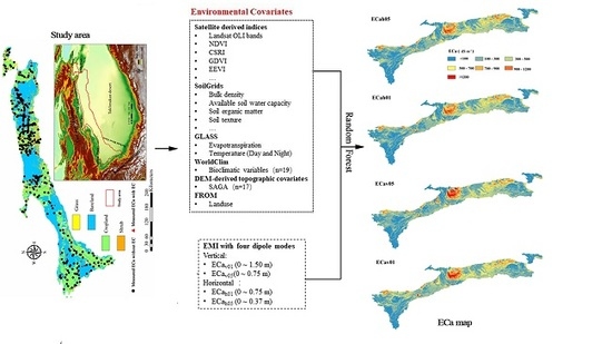
establish quantitative RF–based EMI prediction model (horizontal and vertical modes, ECa, mS·m⁻¹) using RF algorithm and other auxiliary remote sensing environmental products, then,

(2)

predict ECa spatial distribution at the predefined bulk soil depths (0–37.5 cm, 0–75 cm and 0–150 cm) and analyze the spatial distribution characteristics of soil salinity by the predicted ECa maps,

Finally, (3) evaluate this study by analyze on the representiveness of predicted ECa to measured EC and analyze the reason of the differences on the spatial distribution characteristics by the predicted ECa of this study and ECe data of 1980s that achieved from HWSD database.

2. Study Area

This study was conducted in an oasis group of Tarim Basin (latitudes 37°45′47″N and 42°31′430″N and longitudes 77°26′580″E and 86°28′430″E) located between the Tianshan Mountains and the Taklimakan Desert, the most arid region in China (Figure 1). The Tarim Basin belong to Xinjiang located at northwestern China region has an arid climate and fragile ecological environment. Oasis areas account for only ~3–5% of Xinjiang’s area, but support >95% of the population and >80% of social wealth. The established study area (a total area of 572,858 km²) covered seven oases (Yanqi, Korla, Luntai, Weigan River-Kucha, Bachu, Yarkant River and Kashi), which support the most human activity and consume the most water in the Tarim Basin (Figure 1). In this extremely arid climate, the average annual precipitation is 50–100 mm and the interannual evaporation is 2000–3000 mm [45]. The average air temperature from 1961 to 2015 was 7.6 °C. Melting ice/snow from the Kunlun and Tianshan Mountains and precipitation are the main water sources in the area (45–60% and 18–33% of river replenishment, respectively). Historically, all nine major river systems in the Tarim River Basin flowed into the main channel of the Tarim River. However, due to the impact of human activity and climate change, only the Aksu, Yarkant, and Hotan Rivers still supply the Tarim River (the so-called “upstream three source streams”). In the past 60 years, mountain runoff has increased in the upstream source region of the Tarim River, but the amount of water reaching the Tarim River at the Alar hydrological station has decreased significantly [46]. This is mainly due to increased water consumption by increasing human activity in source regions (such as the expansion of oasis farming), which increased from 50 × 10⁸ m³ in the 1950s to 278 × 10⁸ m³ in 2015.

Land use types in the area include farmland, grassland, shrub land, riparian forests, sandy land, saline land and other unused land. The main crop types include cotton, wheat, corn and fruit. Natural vegetation consists of drought- and salt-tolerant shrubs and riparian forests with common species including Tamarix ramosissima, Populus euphratica, Phragmires communis, Poacynum hendersonii and Alhagi sparsifolia. The soil type primarily comprises Haplic Gypsisols, Cumulic Anthrosols, Calcaric Fluvisols, Gypsic Solonchaks and Gleyic Phaeozems according to the harmonized world soil database (HWSD v1.2) (http://www.fao.org/soils-portal/soil-survey/soil-maps-and-databases/harmonized-world-soil-database-v12/en/) [47]. The study area is also characterized by alkalized desert soils or salinized meadow soils. The vegetation types include annual crops and drought-resistant economic crops inside farmlands, include cotton, corn, sunflower, pear, walnut, jujube, beet and various vegetables. Most saline soil in the study area was developed on the basis of loose Quaternary sedimentary parent material. The sloping plains at the foot of the mountain are composed primarily of brown gypsum desert soil. At the lower edge of the oases, salinized soil is common because of the shallow groundwater level and strong evaporation.

3. Data and Methods

3.1. Environment Variables

Soil patterns are formed by the type, intensity and spatial arrangement of land uses as well as underlying environmental landscape properties. The SCORPAN conceptual model provides a framework for quantitative mapping of soils at the landscape scale [48]. In this model soils are predicted as a function of mapped soil properties (S), climate (C), organisms/vegetation (O), relief (R), parent material (P) that are also dependent on age/time (A) and geographic space (N). Our objectives were to apply the SCORPAN model to soil–landscape conditions in Tarim Basin and implement a quantitative ECa-landscape model. All environmental data sets are shown in

Table 1. Land surface parameters used for spatial prediction of ECa.

Auxiliary Data	Land Surface Parameters	Definition	Reference/Source	Soil Forming Factors
SoilGrids (250 m)	CRFVOL	Coarse fragments volumetric in %	[24]	S
	OCSTHA	Soil organic carbon stock in tons/ha		S
	OCDENS	Soil organic carbon density in kg/cubic-m		S
	CECSOL	Cation exchange capacity of soil in cmolc/kg		S,P
	PHIKCL	Soil pH × 10 in H2O		S,P
	SNDPPT	Sand content (50–2000 micrometer) mass fraction in %		S,P
	SLTPPT	Silt content (2–50 micrometer) mass fraction in %		S,P
Remote sensing data (30 m)	Landsat OLI	Band 1–7		P,S,NS,A
	Minimum noise Fraction of OLI bands	MNF1,MNF2,MNF3		P,S,NS,A
	CSRI	Canopy response salinity index	[5]	O
	EEVI	Extended enhanced vegetation index	[51]	O
	GDVI	Generalized difference vegetation index	[52]	O
	CAI	carbonate index	[52]	P,S
	SIT	Salinity index	[53]	P,S
	CI	Clay index	[54]	P,S
	BI	Brightness index	[54]	P,S
Land use (30 m)	Land use	Global 30-m surface land use\cover products (finer resolution observation and monitoring (FROM)	[69]	P,S,O,C
Climate (1 km)	AT	Air temperature	National Earth System Science Data Center	C
	ET	evapotranspiration
	TEM_NIGHT	Night surface temperature
	TEM_DAY	Day surface temperature
	Bioclimatic variables	Bio1, Bio2, Bio3… Bio19	WorldClim
Terrain attributes (90 m)	VD	Valley depth	SAGA GIS	R
	VDCN	Vertical distance to channel network
	TWI	Topographic wetness index
	SL	Slope length
	SVF	Sky view factor
	TPI	Topographic position index
	MRVBF/MRRTF	Multiresolution index of valley bottom Flatness
	SH	Slope height
	NH	Normalized height
	STH	Standardized height
	MSP	Mid-slope position
	TEX	Terrain surface texture
	FA	Flow accumulation
	CSC	Cross-section curvature
	LC	Longitudinal curvature
	RSP	Relative slope position

and unified to a spatial resolution of 90 m by nearest neighbor.

Bioclimatic variables (BIO01—annual mean temperature; BIO 02—mean diurnal range (mean of monthly (max temp–min temp)), BIO 03—isothermality (BIO2/BIO7) (∗100), BIO 04—temperature seasonality (standard deviation ∗ 100), BIO 05—max temperature of warmest month, BIO 06—min temperature of coldest month, BIO 07—temperature annual range (BIO5–BIO6); BIO 08—mean temperature of wettest quarter; BIO 09—mean temperature of driest quarter; BIO 10—mean temperature of warmest quarter; BIO 11—mean temperature of coldest quarter; BIO 12—annual precipitation; BIO 13—precipitation of wettest month); BIO 14—precipitation of the driest month; BIO 15—precipitation seasonality (coefficient of variation); BIO16—precipitation of the driest quarter; BIO17—precipitation of the wettest quarter; BIO18—precipitation of warmest quarter; BIO19—precipitation of the coldest quarter; S—soils; C—climate; O—organisms; R—relief; P—parent material; A—age; N—space).

Of the climatic factors, air temperature, ground temperature and evapotranspiration are important external environment covariates for causes of soil salinization. Temperature data were obtained by interpolation using the ANUSPLIN (Australian National University Spline) method, which takes into account the influence of topographic factors on temperature and is currently recognized as a superior method for meteorological data interpolation. The GLASS evapotranspiration (ET) product is a Bayesian method that integrates five traditional latent heat-flux algorithms (MOD16, improved PM, PT–JPL, MS–PT, and semi-empirical Penman) [49], was used. Temperature and GRASS_ET data were acquired in 2015 from the National Earth System Science Data Center (http://www.geodata.cn/). Day and night surface temperature data from MODIS were also used. Nineteen bioclimatic variables from WorldClim (Bio1, Bio2, Bio3… Bio19) [50] also served as potential predictors. Bioclimatic variables are more environmentally relevant as climate proxy indicators than simply using annual average temperature and precipitation. The bioclimatic variables in these data set were calculated from monthly temperature and rainfall data from 1970 to 2000. These biologically significant variables represented annual trends (e.g., average annual temperature and precipitation) and climatic characteristics under extreme or restrictive conditions (e.g., temperature in the coldest and hottest months and precipitation in wet and dry seasons).

The six bands in Landsat–8 OLI and their derivatives were also used. Prior to deriving the various spectral indices, the Landsat–8 OLI data underwent radiometric calibration and atmospheric correction. The vegetation and soil indices used in this study have been confirmed by many studies as typical indicators for use in soil property prediction and play an important role in soil property modeling; these included canopy response salinity index (CSRI) [5], extended enhanced vegetation index (EEVI) [51], generalized difference vegetation index (GDVI) [52], salinity index (SIT) [53], Clay index (CI) [54], brightness index (BI) [54]. Minimum-noise fraction (MNF) components (MNF1, soil-moisture-related; MNF2, vegetation-related; MNF3, bare-soil-related) transformed from Landsat-8 OLI data were also considered.

Under different land use patterns, the differences that in hydrothermal conditions have significant effects on water and salt transport, therefore, land use were chosen as auxiliary identification data. The product used in this study are 30-m global surface land use/cover product, the selection version is 2017, product details may be found in Gong et al. [55]; the download address is http://data.ess.tsinghua.edu.cn/. The Level1 land cover types of this product are farmland, grassland, shrubbery, desert, unused land, urban land and water bodies.

SoilGrids provides global predictions for standard numeric soil properties (organic carbon, CEC, pH, soil texture fractions, available soil water capacity and coarse fragments) at seven standard depths (0, 5, 15, 30, 60, 100 and 200 cm) [24]. This study’s ECa modeling used six SoilGrids products as environmental covariates. Each product contained seven standard depth values (0, 5, 15, 30, 60, 100, 200 cm), adding an adjacent depth for each predicted depth to avoid producing unexplained results. For example, an ECa_h05 prediction model at a depth of 0–37 cm used SoilGrids products at 0 and 30 cm. At the same time, the products were marked by depth; for example, BD_1 and BD_4 were the bulk density at depths of 0 and 30 cm, respectively.

The DEM-derived topographic covariates indicated (directly or indirectly) the direction of movement of the parent material and water while suggesting the location of accumulated soil salts. The topographic fluctuations directly affect the transportation and distribution of surface and underground runoff. Terrain-derived covariates were employed in this study with a spatial resolution of 30 m (Table 1). A 30-m DEM (ASTER GDEM V2) was downloaded from the Geospatial Data Cloud (http://www.resdc.cn) and preprocessed with mosaicking and sink filling using SAGA (System for Automated Geoscientific Analyses) GIS software.

3.2. Field Sampling

Sampling locations (Figure 1) were determined using the conditional Latin hypercube sampling (cLHS) [56] design method based on a wide range of environmental covariates: climate (air temperature, precipitation and evapotranspiration), vegetation (CSRI, GDVI, EEVI), topography (MRVBF, MRRTF), soil–related indices (SIT, CI, BI) and CAI [52]) and land use type.

Field measurements were conducted during 2 to 17 August 2018. The locations of some unreachable samples were adjusted by considering accessibility and the soil landscape’s spatial variability. Sample density was increased in the oasis-desert areas south of Luntai Oasis and east of Kuqa Oasis, as landscape types typical of the study area were common in these areas and the traffic roads are relatively dense. In this campaign, ECa was measured at 474 locations, of which 132 individual sites were visited according to local landscape and soil was sampled at multiple depth (0–10 cm, 10–20 cm, 20–40 cm, 40–60 cm, 60–80 cm and 80–100 cm). In actual field sampling, try to ensure that the soil landscape inside each plot (90 * 90 m) is relatively homogeneous.

An EMI survey was conducted used electromagnetic instrument (EM38-MK2) for soil sensing developed by Geonics, Ltd. (EM38MK2, ON, Canada), along a non-linear path at time intervals of ~5 s with 2-minute-long in each study plot. The instrument was carried at a height of 5 cm above the ground surface. Before each measurement, the instrument was calibrated at 1.5 m above the ground with a PVC ladder, following the study of McNeill [57]. Any metallic objects were avoided during the survey. EMI readings were conducted in both vertical (V, ECav, mS·m⁻¹) and horizontal (H, ECah, mS·m⁻¹) dipole mode, the specific measurement depths are: 0–1.50 m (ECav01) and 0–0.75 m (ECav05) for the V mode and 0–0.75 m (ECah01) and 0–0.375 m (ECah05) for the H mode [58], separately. ECa measurement points numbered 400–650 per study plot. The average of reads of four dipole modes was taken as the last observation at each plot.

The preliminary ECa data were downloaded to a spreadsheet and subjected to preprocessing. First, stationary measurements were identified and removed (particularly at the beginning or end) by viewing the ECa data as a time series and deleting values of 0 and nearby low values by checking the data against the GPS speed. Negative values were also removed together with surrounding data. Temperature correction was also needed; based on the average soil temperature at a depth of 0.5 m, an equivalent of 25 °C was chosen to standardize the ECa values using a widely accepted formula [59]:

ECa_{25 °C} = ECa * (0.4779 + 1.3801e^{(−T/25.654)})

(1)

Of the 474 sampling points, the temperature of the 0–100-cm profile at 132 points was measured. After calculation, it is found that the difference between the average temperature of 0–50 cm and the average temperature of 0–100 cm is about 2%. In addition, the temperature has relatively little influence on ECa and in order to improve the sampling efficiency, the average temperature of 0–50 cm is collected for the remaining 342 points.

Electrical conductivity (EC, mS·m⁻¹) was measured at 25 °C with a LeiCi DDS-307 (ShengKe, Shanghai, China) conductivity meter on a 1: 5 soil: water extraction of each sample created according to experimental literature [60]: the air-dried, ground and sieved (0.5 mm) soil samples were mixed with water with a 1:5 (weight: volume) ratio at room temperature (25 °C). Grind the air-dried sample, use a 0.5-mm-pore-size filter with a sieve to prepare a standard temperature of 25 °C, extract the extract according to the ratio of soil to water 1:5 and measure the soil electrical conductivity EC1:5 and soil salinity.

3.3. Machine Learning Algorithms

3.3.1. Random Forest

To construct the RF relationships between ECe and environmental covariates, the random forest package in statistical software R was used [61]. The RF classifier uses numerous decision trees, ntree, that are grown from bootstrap samples (63%) from the entire sample population, n [62]. RF modeling requires three user-defined parameters: the number of covariates used to grow each tree (mtry), the number of trees in the forest (ntree) and the minimum number of terminal nodes (nodesize). The RF classifier uses a bootstrapped sample to create decision trees. At each binary split, the predictor that produces the best split is chosen from a random subset, mtry, of the entire predictor set, p, where the number of predictors tried at each split, mtry, is defined by the user. As a result, mtry is recognized as the main tuning parameter of RF and should therefore by optimized [63]. The use of bootstrap sampling in RF modeling allows the remaining unused subset (37%, i.e., the out-of-bag data (OOB)) to be used for the estimation of general errors. RF predictions are the averaged output of all aggregations. The default mtry value of random forest relates to p/3. However, in the case of RF, this is particularly true for datasets with correlated predictor variables, for which several mtry values should be considered [64]. To optimize the primary tuning parameter, mtry values ranging from 1 to 30 were tested, and the OOB error rates from 50 replicates from each mtry value were assessed. Then, mtry were further assessed using RMSE (root mean squared error) obtained from the replication of a 5-fold cross-validation. Nodesize = 5 was used. The default value for the number of trees (ntree, 200) proved to be insufficient to yield stable results [65]. Therefore, we set ntree = 1000 for the test that applied to the RF model.

3.3.2. Variable Selection

Variable reduction has been previously used to reduce errors in predictions [63] through the removal of potentially irrelevant predictor variables. This process progressively increases the accuracy of the prediction by reducing the chance of obtaining outliers since weak learners also produce weak outliers. This study utilized recursive feature elimination (RFE) [66] to identify the minimum dataset (with relatively low errors) from all covariates. This method identifies the minimum dataset by building a prediction model with all predictor covariates, uses variable rankings to eliminate the least important predictor, and repeats until only a single variable remains. Variable reduction approaches include correlation-based feature selection [67] and utilization of the RF algorithm to select covariates based on variable importance metrics. In this study, RF was used to calculate the importance of the predictors because it is not highly sensitive to data distribution [68]; the optimal subset was identified using the minimum OOB error.

3.4. Model Validation

Each ECa model data set was assigned a calibration set (342 samples, 70%) and a validation set (132 samples, 30%) based on the cLHS. In order to ensure model stability and increase reliability, this study adopted the nonparametric bootstrap [69]. The aim was to guarantee credibility of the predicted value, where the procedure was repeated 10 times using 70% of the sampled data. The mean estimates of soil salinity from 10 times RF predictions then represented as the final result for each model. Finally, we refitted the best model with all 474 observations to predict the ECa within unknown areas of the 90 m grid. The coefficient of determination (R²) was used to assess variation and correspondence between the predictions and original data, while the root mean squared error (RMSE) was used to quantify the inaccuracy of the predictions. The formula for calculation of these indices and their applicability in soil attribute mapping can be found elsewhere [70]

$$R^2={[\frac{{\displaystyle {\sum }_{i=1}^{\mathrm{n}}(O_i-P_{ave})(P_i-P_{ave})}}{{\displaystyle \sum _{i=1}^n{(O_i-P_{ave})}^2{(P_i-P_{ave})}^2}}]}^2$$

(2)

$$PMSE=\sqrt{\frac{{\displaystyle \sum _{i=0}^n(O_i-P_i)}}{n}}$$

(3)

where O_i is the observed value, P_i denotes the predicted values, O_ave and P_ave shows the average of observed and predicted values, n is the number of data.

4. Results

4.1. Statistical Description of ECa and EC Data

The statistical characteristics of ECa varied in vertical and horizontal dipole mode (

Table 2. Statistical summary of the four ECa coil configurations and electrical conductivity (EC) at six depths.

ECa/EC	Min	Max	Mean	SD	CV
ECah05	0.98	1292.41	329.45	315.10	1.18
ECah01	1.53	1279.92	325.86	310.89	1.17
ECav05	0.67	1898.60	350.14	336.87	1.15
ECav01	1.39	1763.94	354.43	338.12	1.11
EC0–10 cm	0.08	88.35	7.27	12.75	1.75
EC10–20 cm	0.07	29.15	4.19	6.20	1.48
EC20–40 cm	0.05	21.23	3.33	5.14	1.54
EC40–60 m	0.06	18.88	2.96	4.47	1.51
EC60–80 cm	0.05	15.20	2.30	3.48	1.51
EC80–100 cm	0.07	13.75	2.08	2.94	1.41

CV: coefficient of variation; SD: standard deviation; ECa (mS·m⁻¹); EC (dS·m⁻¹).

). Both the maximum and minimum values appeared in ECav05. The average values of ECav05 and ECav01 were higher than ECa_h05 and ECah01, which was related to the continuous increase of total amount of soil water content from top to bottom layer in the study area, relatively [71]. Bennett and George [72] and Mcfarlane and Ryder [73] reported that moisture content plays an important role in electromagnetic induction measurements. Misra and Padhi [74] assessed field-scale soil water distribution by EMI, as increasing soil water would promote a high degree of confidence (P < 0.01) and coefficient of determination (R² = 0.6–0.7) for the fitted models of ECa-soil water. As the depth increased, the coefficient of variation (CV) of ECa gradually decreased, the maximum value appeared in ECa_h05, and the minimum value appeared in ECa_v01. This is because of biophysical heterogeneity in surface soil is higher than in deep layer. The CV coefficients of the four ECa coil configurations exceeded 100%, suggesting that the combination of water and salt in this area exhibited strong spatial variability according to Wang et al. [75]. The distribution characteristics of the ECa data in this study were similar to the distribution range of ECa values measured for four typical land uses in the Aksu Oasis [76].

As the depth increases, the average value of EC tends to decrease (Table 2). The maximum value appears in the surface layer, with value of 88.50 dS m⁻¹. From 10–20 cm to 80–100 cm, the average value are 7.27 dS·m⁻¹, 4.19 dS·m⁻¹, 3.33d S m⁻¹, 2.96 dS·m⁻¹, 2.30 dS·m⁻¹, 2.08 dS·m⁻¹. Handbook 60 (US Salinity Laboratory Staff, 1954) defines various general categories of soil salinity [77]: 0–2 dS·m⁻¹ (non-saline), 2–4 dS·m⁻¹ (slightly saline ), 4–8 dS·m⁻¹ (moderately saline), 8–16 dS·m⁻¹ (strongly saline) and >16 dS·m⁻¹ (extremely saline). According to this classification, the soils at all depths are subject to different degrees of soil salinization and show obvious surface aggregation. This is due to the continuous loss of water and the accumulation of salt during the rise of groundwater under strong evaporation. The CV value of EC at all depths exceeds 100% (CV lower than 0.1, indicating low variability while CV higher than 1.0 indicates great variability) [75], where the maximum value is 1.75 in 0–20 cm, and the minimum value is 1.41 in 80–100 cm, That is, the depth increases while the CV value decreases sequentially, which indicates strong spatial variability with respect to soil salinity in the study area.

Dividing ECa (ECav01 and ECh05) samples into 3 groups (farmland, shrub/grassland, bare land) and calculated their box plots (Figure 2). The statistical results show that the average values of ECah05 and ECav01 of bare land (481.10 and 483.35 dS·m⁻¹) are higher than those of shrub/grassland (366.73 and 336.96 dS·m⁻¹) and farmland (100.05 and 108.91 dS·m⁻¹). Most of the samples in bare land are collected in highly salinized areas, where the groundwater level is latent (1–3 m) and the soil type belongs to solonchak. The outliers in farmland areas are caused by improper farmland managements and abandonment of wasteland accompanied with soil salinization. In addition, as the salinity level continues to increase (from non-saline 0–2 dS·m⁻¹, 2–8 dS·m⁻¹, 8–16 dS·m⁻¹ to >16 dS·m⁻¹), the average values of ECah05 and ECav01 increase in sequence, which are 58.69, 212.51; 325.17, 585.99; 68.95, 206.56; 279.13, 597.04 dS·m⁻¹. The reason the value of ECav01 is higher than that of ECah05 is that the measured profile depth of the former is twice that of the latter, therefor the content of water and salt is higher.

4.2. Correlation between ECa and EC at Different Depths

The Pearson correlation coefficient (r) among EC at all depths is significant (p < 0.01) (

Table 3. Pearson’s correlation coefficient among soil salinity at different depths (n = 132).

Depth	EC0–10 cm	EC10–20 cm	EC20–40 cm	EC40–60 m	EC60–80 cm	EC80–100 cm
EC0–10 cm	1.00 **
EC10–20 cm	0.83 **	1.00 **
EC20–40 cm	0.71 **	0.94 **	1.00 **
EC40–60 m	0.67 **	0.90 **	0.95 **	1.00 **
EC60–80 cm	0.71 **	0.88 **	0.91 **	0.93 **	1.00 **
EC80–100 cm	0.58 **	0.81 **	0.85 **	0.90 **	0.89 **	1.00 **

**: p < 0.01.

). The r value between surface EC (0–10 cm) and other depths from lower to deeper are 0.83, 0.71, 0.67, 0.71 and 0.58; the correlation between EC (10–20 cm) and EC at other depths in sequence are 0.94, 0.90, 0.88 and 0.81. The r value between EC (10–20 cm) and EC at other depths is above 0.85. The aforementioned results indicate that there is a linkage between the changes of EC at different depths, that is, the area where the surface soil salinity is high, the probability of a high salinity value in the deep profiles of its location will also be relatively high. This phenomenon has been repeatedly demonstrated by previous study such as Li et al. [78] and Lv et al. [79] in the oasis located at Xinjiang.

Table 4. Pearson’s correlation coefficient between ECa and EC at different depths and land use types.

Land Use	ECa/EC	EC0–10 cm	EC10–20 cm	EC20–40 cm	EC40–60 m	EC60–80 cm	EC80–100 cm
Farmland	ECah05	0.72 **	0.64 **	0.56 **	0.55 **	0.57 **	0.45 **
	ECah01	0.75 **	0.70 **	0.57 **	0.56 **	0.61 **	0.50 **
	ECav05	0.63 **	0.61 **	0.57 **	0.55 **	0.58 **	0.52 **
	ECav01	0.74 **	0.73 **	0.65 **	0.64 **	0.66 **	0.57 **
Shrub/grass	ECah05	0.29	0.40 **	0.57 **	0.54 **	0.56 **	0.34 *
	ECah01	0.35 *	0.40 **	0.58 **	0.53 **	0.64 **	0.47 **
	ECav05	0.37 *	0.43 **	0.64 **	0.63 **	0.56 **	0.40 **
	ECav01	0.37 *	0.44 **	0.65 **	0.64 **	0.62 **	0.53 **
Bare land	ECah05	0.33 *	0.63 **	0.66 **	0.66 **	0.63 **	0.61 **
	ECah01	0.36 *	0.70 **	0.74 **	0.75 **	0.71 **	0.68 **
	ECav05	0.36 *	0.64 **	0.71 **	0.69 **	0.66 **	0.62 **
	ECav01	0.41 *	0.71 **	0.77 **	0.76 **	0.72 **	0.68 **

**—p < 0.05; *—p < 0.01.

shows the correlation between ECa–EC. Taking land use types as an example, the ECa–EC correlation in bare land is relatively highest. Comparing the ECa–EC relationship at different depths, it is found that the shallow correlation (0–20 cm) in farmland area is relatively highest (r = 0.75), and the maximum correlation appears at 20–40 cm within shrub/grassland (r = 0.65) and bare land (r = 0.77). In addition, among the four ECa models, the correlation of ECav01–EC is the highest among all land types. At the same time, it was also found that the sensitivity of ECa to EC is on the surface of farmland, but in the deep layer of non-farmland. Similar results were also found by Wu et al. (2019) [80], which conducted EMI soil salinity local modeling research within Alear Oasis at southern Xinjiang and the soil samples mainly collected at the two typical desert and farmland classification in July, 2017, their results showed that regardless of the degree of soil salinization are slight, moderate or severe, the correlation between EC and ECa is relatively lower at the surface layer while the higher value showed in the deep layer. The correlation of ECa–EC in the surface layer is weaker than that in the deep layer, which may be due to the low moisture content of the surface layer, which is not conducive to EMI perception of changes in soil properties [81]. Nevertheless, considering the high correlation between ECa and EC (10–80 cm) and the close linkage between EC (10–80 cm) and EC (0–10 cm), it implies that ECa still has a strong indication for EC changes for the soil profile.

4.3. Important Variables

The dominate contributor for the four ECa models were identified by the RF algorithm using RFE (Figure 3). Normalizing the contribution of the preferred covariates to 100% and the relative importance of single covariates for all models showed in Figure 3. The main control factors for horizontal dipole mode was soil-related variables, shows 42.69% in ECa_h05 and 37.36% in ECa_h01 and for vertical dipole mode was climate-related variables, shows 34.51% in ECav05 and 41.22% in ECa_v01. At each dipole mode, as the depth down from shallow to deep profile, the influence of soil-related covariates decreased from 42.69% to 37.36% at horizontal and 33.50% to 29.38% in vertical, vegetation covariates reduced from 31.53% to 26.87% in horizontal and 31.99% to 29.40% in vertical, while the climate-related contributors appeared opposite trend, with an number up to 38.33% come from 25.87% in horizontal and 34.51% to 41.22% in vertical. Climate is the main traction force for the vertical movement of water and salt in the soil profile [32]. Babaeian et al. [82] and Toby [83] have showed that the most important parameter affecting spatial variability of soil moisture is land surface temperature. In the long term, vegetation and soil are relatively stable.

For all the four ECa models, the primary two predictors confirmed by RF are MNF2 (highly correlated with vegetation information in this study) and temperature at night (TEM_NIGHT) and MNF2 taken the first position at ECah05, while temperature is the most important variable at the left three models. Then, the followed important predictors are: SIT for both h01 and v01 mode, land use for V05 and SNDPPT_4 for h05. All of these predictors mentioned have over 40% of relative importance at each model, at least. In specific, surface temperature at night for the climate variables, MNF3 and SIT (surface reflectance) and the proportion of sand for the soil variables and MNF2 for the vegetation-related covariates were the mainly contributors.

In addition, the SoilGrids dataset contributed 20.00% to the ECa_h05 model, followed by ECa_h01 (13.28%), implying that SoilGrids was more sensitive to changes in surface properties than deep ones. Coincidentally, the results of variable importance from study of Liang et al. [84] show that SoilGrids data were the best predictors for defining the soil-landscape relationship during regression modeling for oil organic carbon. Hengl et al. [24] reported that SoilGrids is not expected to be as accurate or relevant as locally produced maps but can be used as an important variable in the construction of local models.

4.4. Correlation between Environmental Covariates and Measured ECa

The correlation between selected environmental covariates by RFE and ECa was significant at p < 0.01 (Figure 4). Although the ranking order was different, the top three covariates that positively correlated with ECa were similar (TEM_NIGHT, B2, B1/Land use/B3), due to the high correlation between the four ECa coil configurations. The most relevant variable in all four ECa modes was TEM_NIGHT, with correlation coefficients after rounding of R² = 0.57. This is consistent with the fact that soil moisture information reflected by night temperature (closely related to thermal inertia) is the main limiting factor for landscape spatial heterogeneity in arid areas. The covariates related to vegetation indices (CSRI, EEVI, GDVI and MNF2) and evapotranspiration (ET) were all negatively correlated with ECa. These relationship was proved by Taghizadeh-Mehrjardi et al. [54] and Scudiero et al. [5] who pointed over-accumulated salt in soil will suppress vegetation growth and reduce coverage and biodiversity [85], subsequently, decreased the total amount of evapotranspiration [32]. For ECah05 and ECah01, the largest negative correlation coefficients were SLTPPT_4 (r = −0.50) and CSRI (r = −0.48), respectively. The largest negative correlation coefficients were all ET with r = −0.47 and r = −0.49, respectively, for ECav05 and ECav01. Rainfall-related covariates and ECa were weakly related, such as BIO15 and BIO12. Limited and unevenly distributed rainfall in this area greatly weakened indications of its redistribution with regard to soil salinity [86]. The correlation between SNDPPT and SLTPPT from the SoilGrids dataset and ECa was significant at p < 0.01, indicating that these parameters can be used for the interpretation of local water and salt changes.

4.5. Calibration and Validation of the ECa Model

All calibration and validation RF-ECa models were highly significant (p < 0.001) (Figure 5 and Figure 6). The calibration model had an R² range of 0.68–0.71 and an RMSE range of 205.65–227.83 mS·m⁻¹ (Figure 5), while the validation results had an R² range of 0.77–0.84 and an RSME range of 115.17–142.76 (Figure 6). The best validation accuracy was achieved using data from ECav05, possibly due to the wider ECa range which covered more knowledge with respect to ECa–landscape relationship. The validation results of this study are better than Taghizadeh-Mehrjardi et al. [54], the training-based prediction (80% of the data, R² = 0.75 and 0.69 in vertical and horizontal mode, respectively) and independent validation data set (20% of all data) showed more reasonable results with R² values around 0.49 on the validation dataset. This may be related to the type and number of covariates used in prediction of soil salinity. Such as the various key physical and chemical attributes from SoilGrids dataset with multiple depths and bioclimatic parameters from WorldClim enrich the information dimension of surface heterogeneity. The validation accuracy of the deeper EMI coil configurations (ECa_h01, ECav05 and ECav01) provided generally better predictions of average ECa than the shallower ECah₀₅ as the former integrated a thicker portion of the subsurface. Specific reasons for this include (1) the coefficient of variation of ECa_h05, which was higher near the surface than at other depths and (2) the complex surface and lower soil moisture content, which reduced the correlation between ECa and external environmental covariates. On the contrary, soil depth of 40–100 cm was the main distribution area for vegetation roots and soil moisture (increasing with depth), caused by groundwater-dependent ecosystem [87]. Li [88] also showed that the landscape pattern in arid areas was significantly affected by deep water and salt in dryland areas.

The prediction ability of the ECa model is investigated based on land use (

Table 5. Summary of the performance of ECa model in farmland, shrub/grass and bare land according to R² and RMSE.

Land Use	Ecah05		Ecah01		Ecav05		Ecav01
	R2	RMSE	R2	RMSE	R2	RMSE	R2	RMSE
Farmland	0.43	115.57	0.48	126.27	0.49	116.52	0.44	115.62
Shrub/grass	0.57	171.49	0.77	138.07	0.66	124.77	0.74	111.23
Bare land	0.84	151.27	0.88	129.27	0.89	143.24	0.91	120.70

). Through comparison, it is found that the prediction accuracy of ECa in the bare land area is relatively highest (the R² values in the four ECa models are 0.84, 0.88, 0.89 and 0.91, respectively). The predictive power of ECa values in farmland areas is relatively lowest (the R² values under the four ECa models are 0.43, 0.48, 0.49 and 0.44, respectively). The predictive power of ECa located in shrubs and grasslands lies between them. For the detect depths, both the bare land and shrubs and grassland have a better accuracy with R² all over 0.74 at 1-m depth (ECah01 and ECav01).

4.6. Spatial Distribution Characteristics of ECa

Based on all samples, this study established an RF model for simulating the Eca of oasis agroecosystems and desert-oasis ecotones. The average values of the two vertical modes (Ecav01 and Ecav05, 312.32 and 296.05 mS·m⁻¹, respectively) were generally higher than those of the horizontal modes (Ecah01 and Ecah05, 280.06 and 282.89 mS·m⁻¹, respectively), roughly consistent with the statistical distribution of the observed data. The spatial distribution of the predicted results (Figure 7) showed that pixels with Eca values greater than 1200 mS·m⁻¹ were mainly located in southern Luntai Oasis, eastern Kuqa Oasis, eastern Aksu Oasis and northern Kashi Oasis. These areas were also marked as having highly salinized soil due to the presence of solonchak (a saline–alkali soil) revealed by previous studies in southern Luntai Oasis [89], southeastern and western Kuqa Oasis [75] and eastern Aksu Oasis [90]. Pixels with Eca values in the 500–1200 mS·m⁻¹ interval were primarily distributed around pixel with values > 1200 mS·m⁻¹. Pixels with Eca values in the 100–500 mS·m⁻¹ interval were mainly distributed within oasis areas. Pixels with ECa values < 100 mS·m⁻¹ were concentrated in farmland within individual oases and in desert land (dry soil and low soil salinity).

Figure S1 (in the Supplementary Materials) shows the relationship between ECa measured in this study and historical soil salinity data (ECe from HWSD at the depth of 0–30 cm and 30–100 cm, named ECe_HWSD_030, ECe_HWSD_30100) (Figure 8). The extractive observations from HWSD based on current samples show that the maximum, minimum and average values of ECe_HWSD_030 and ECe_HWSD_30100 are 42.80 and 32.20 dS·m⁻¹, 0.1 and 0.1 dS·m⁻¹, 13.74 and 12.94 dS·m⁻¹, respectively. From this statistical data we can see, the artificially induced soil salinity and natural salinization covered the whole range from non-saline (ECe < 2 dS·m⁻¹) to extremely saline soils (ECe > 16 dS·m⁻¹) [77] and the average values revealed the universality and severity of soil salinization in that era. The soil salinity of the surface layer is higher than that of the deep layer, which is consistent with the distribution characteristics of the statistical results of saline soil of China [7] and soil in Xinjiang [91]. Scatter plot presented ECa was significantly correlated with ECe_HWSD_030 (p < 0.01) and ECe_HWSD_30100 (p < 0.01), the average correlation coefficient of the latter (r = 0.556) was higher than the former (r = 0.482) (Figure S2). This result suggested that HWSD had a certain degree of interpretation of the current pattern of soil water and salt in the range of 0–1.5 m, but it also implies that the distribution of soil water and salt has undergone large changes since 1980s.

These spatial patterns of ECa were similar to the ECe values in the HWSD v1.2 database (Figure 8). In particular, the spatial distribution of soil salinity ECe > 30 mS·m⁻¹ in the 1970s and 1980s from HWSD had a high degree of overlap with the spatial distribution of salinity ECa > 1200 mS·m⁻¹ in this study, but the former covered a larger area. This result may imply that the level of soil salinization in the study area has declined.

5. Discussion and Perspectives

For soil salinity quantification modeling, the relationship between EMI derived ECa and laboratory-analyzed EC were confirmed by previous studies: in the California archives R² = 0.87 with EC (soil:water-1:5) [27], in Australia with R² = 0.92 [92], in Spain with R² = 0.88 and 0.94 in 2009 and 2011, respectively [29], in the Yellow River Delta with R² = 0.86 [30], and in Xinjiang with R² = 0.85, 0.75 and 0.95 for three fields of Chenopodiaceae and Tamaricaceae [31]. This result showed that the ECa-EC correlation is generally lower than the aforementioned studies. Soil salinity is a highly spatiotemporal variability soil property, which related to the distribution characteristics of soil moisture, texture and structure etc. On the whole profile, especially under different land use types on a large landscape scale. Additionally, EMI derived ECa is a depth-weighted composite value for the volume soil. According to McNeill’s research [57,58], the contribution of soil properties within 40 cm on top of the profile is significantly higher than the lower 0.40–1.5 m. In this study, surface layer showed a relatively lower correlation between ECa and EC and the higher correlation are in 10–80 cm totally, this due to the soil moisture is the main factor that impacted the EMI readings in field. Previous studies showed that higher water content appeared in the deep layer in this area [93]. Therefore, the water–salt distribution characteristics and the calculation method of ECa measurements weaken the correlation between ECa and EC. According to the results in Table 4, ECav01 has the strongest ability to detect EC, therefore, the overall soil salinity value in the range of 0–1 m should be supplemented in the future field campaign. Even so, EMI is still the ideal instrument and made the ECa as a better indicator for quickly detecting changes in soil water and salt in profile without destruction of soil structure.

The ECa accuracy of bare land is higher than grass/shrubs land and farmland. Bare land includes sand, Gobi desert and saline-alkali land, which all with a relatively lower vegetation coverage at the surface. The spectral and salinity characteristics of the sand, Gobi and saline–alkali land contained in the bare land are significantly different from each other. In addition, the wide range of ECa/EC value distribution in reality is conducive for obtaining more soil-landscape interaction, which is beneficial to improving ECa modeling accuracy. At the depth of 10–80 cm in profile, the correlation between ECa and EC is around 0.7, indicating that ECa better represented the soil salinized characteristics in bare land. For farmland, frequent and regular irrigation strategies and agricultural management practices dominated the inherent spectrum characteristics of soil. Agricultural activities that artificially increased crop yields with the purpose of economic profits, such as salt-leaching and using organic fertilizer, both made the soil salt content relatively keeping in a lower status within the crop growth area (1 m) on the profile. Especially in the arid irrigation area, soil moisture is the main control factor for vegetation growth [5]. Coupled with the sheltering effect of vegetation, the information loss of indirect acquisition of soil characteristics based on vegetation weakens the modeling accuracy of ECa in farmland. For shrub land and grassland, which have obvious seasonal growth characteristics and different water use strategies. Herbage with shallow root systems tend to use shallow water, while shrubs that have well developed root systems preferred to the underground water in deeper, which made obvious differences on water and salt characteristics in profile. Therefore, the total correlation between ECa and EC within range of 0.29–0.65, especially at 20–80 cm (the overlap growth interval for grassland and shrub) is around 0.6 and ECa modeling accuracy R² is 0.57–0.74. In addition, ECa and EC would present more complicated relationships with difference land landscapes in reality. Other factors that would affect ECa modeling accuracy are as follows: different combinations of vegetation types, pests and vegetation diseases at a single pixel scale and the spectrum noise caused by the severe salinization inside some farmland plots and so on.

Vegetation and temperature are the main contributors to the spatial change of ECa (change in water and salt) in the study area. Vegetation in this area mainly depend on shallow soil water and shallow groundwater to survive [17], which made it a great indicator for the soil and the climate change [94] and a better indirect proxy for the soil salinity based on its convince at remote sensing monitoring [75]. Previous studies had identified a relationship between land surface temperature (LST) and normalized difference vegetation index (NDVI) and described a triangular shape for the data falling between these axes [95,96]. Based on this, a temperature vegetation dryness index (TVDI) was developed for soil moisture detection in Senegal [97]. More comprehensive reviews of the application of remotely sensed LST/vegetation indices for the estimation of soil surface moisture and evapotranspiration can be found in Carlson et al. [98] and Li et al. [99]. Among the environmental parameter sets, land surface temperature showed the highest impact on the spatial distribution of soil water in the Iran which had similar landscape to our sites. A general knowledge is that soil water content were the one of main drivers for salt ion moving in soil. A linear regression model demonstrated that soil water and salt could explain ~83% of variance in ECa values within the Qinghai-Tibet Plateau [100]. Other studies revealed a higher sensitivity of ECa to soil moisture when soils were wet [101]. Robinet et al. [102] found that deeper ECa could best predict the variability of soil water content using a non-linear relationship in southern Brazil. In Tarim river basin, ET is the key response factor for soil moisture and surface temperature which is enhanced by increasing net radiation and that also associated with warming atmosphere [103], favors the process of ET [94]. Mao et al. [104] used several years of experiments in the Yarkant River basin, Xinjiang, to show that the amount of phreatic evaporation from bare soil was closely related to factors including atmospheric evaporation capacity, soil texture and groundwater depth. Li et al. [94] concluded that solar radiation intensity, temperature and humidity had important effects on phreatic evaporation. In the driest condition (lowest moisture), thermal conductivity is associated with the salt amount-salinity [52]. These studies fully verified the closed logical relationship among water, salt and temperature.

The results showed that the predicted ECa maps have an explanation of 0.19–0.7 for the spatial variation of measured EC based on Table 4 and Table 5. Considering the correlation between ECa-EC and the modeling accuracy of ECa, the R² range of farmland is 0.19–0.36 (mean value is 0.28), grassland is 0.16–0.49 (mean value is 0.34), and bare land is 0.28–0.70 (mean value is 0.56). Among them, the predictive ability of ECav01 is more worthy of attention for all land use types. The modeling accuracy of farmland and grass land and shrub are lower than bare land, which means that the improvement of modeling accuracy on the former two land use types need to be done in the following ways in the future: (1) Make sufficient samples collection in farmland and grassland and shrub, use multi-period remote sensing data and land use products with higher spatial and temporal resolution; (2) Compared to single image data, multi-period remote sensing data could provide more information in each pixel. For example, single-period images could not better deal with different object with the same spectra characteristics, asymmetry of surface landscape and soil properties and non-periodicity (randomness) of external interference. For this, the Department of Earth System Science of Tsinghua University has released a new generation of earth observation data: seamless remote sensing observation data (seamless data cube, SDC) with a resolution of 30 m (daily data, 2000–2018). SDC is strongly supported by Amazon Cloud Services (AWS), which could make up for the shortcomings mentioned above for the single-period images, low-temporal resolution images, exploration need to be done in the future.

While shifts in farmland expansion and climate change were likely responsible for the differences of these two soil salinity baselines, the inconsistencies of sample sizes and ECa mapping methods tended to contribute to the uncertainties associated with the comparisons. (1) Since 2001, the proportions of cultivated land, grass and shrub land and bare land are 21.54%, 33.80%, 2.12% and 42.54% respectively. Moreover, in 2017, the ratio changed to 37.72%, 4.79%, 3.90% and 53.59%. In total, from 2001 to 2017, the area of cultivated land, shrub land and bare land were increased by 16.18%, 1.78% and 11.05% respectively, and the proportion of grassland has dropped approaching 30%. As previous studies reported, the annual average precipitation of this area has decreased since 2000, under the climate change condition, and station observation data showed that nearly half of the station measured precipitation showed a downward trend [21].The temperature of this area has been increasing since 2000, resulting a more intensive evaporation and serious loss of soil moisture [105]. These are not conducive to the shallow-rooted natural vegetation’s survival, for its weak drought resistance. Highly intense human activities, such as reclamation on natural land and regular irrigation of artificial crops, which directly changed the characteristics of land cover, soil physical and chemical properties and soil water dynamics, to a certain extent. The water and salt dynamic information that caused by these land use changes, cannot be derived from HWSD data. (2) The source data that HSWD database used for EC mapping only contained 30 sites for this study area [106], and the site data are derived from the national land survey in 1980s, outdated for the recent years. Our study collected 474 samples in the whole region, covering the main typical land use types, which can better represent the changes of natural and human-made landscapes. In addition, the soil salinity in the HWSD baseline was estimated by extending the sparse soil profiles according to soil map units. The soil map units were usually much coarser than the 1 km resolution adopted by HWSD and tended to be inconsistent with the spatial units of soil management practices, climate and land use changes. Consequently, the soil salinity predictions were inaccurate for those fine cells with similar soil management practice/land use characteristics but located in different soil map units. The large difference in the sampling data sizes could lead to different estimation accuracies, particularly at fine resolutions, with small sample sizes generally leading to higher mapping uncertainties [107]. While high uncertainties emerged in fine scale comparisons, the spatial patterns of the mapped ECa were generally consistent with the spatial distributions of the measured soil salinity and land use at large scales (Figure 1 and Figure 7). Given the current data availability, the comparison of these two soil salinity baseline provided valuable information on soil salt changes in southern Xinjiang.

6. Conclusions

This study used EMI observation data and machine learning algorithms to predict soil ECa and analyze its variations in spatial distribution in oasis agroecosystems and desert-oasis ecotones, taken the Tarim Basin of Xinjiang, China as a case study. All four EMI dipole modes based on RF showed good prediction results, though the ECa accuracy in vertical mode was a little bit better than that in horizontal mode. It is found that the shallow correlation (0–20 cm) in farmland area is relatively highest (r = 0.75), and the maximum correlation appears at 20–40 cm within shrub/grassland (r = 0.65) and bare land (r = 0.77). In addition, among the four ECa models, the correlation of ECav01–EC is the highest among all land types. Considering the correlation between ECa–EC and the modeling accuracy of ECa, the R² range for farmland is 0.19–0.36 (mean value is 0.28), for grassland is 0.16–0.49 (mean value is 0.34) and for bare land is 0.28–0.70 (mean value is 0.56). Compared to the EC within the HWSD dataset, the ECa predicted by this study had a similar pattern with it in spatial distribution characteristic and supplied more detail information in raster image with specific digital values. The prediction mapping method presented here can be used as an important alternative way for identifying high water and soil salinity for other similar dryland areas throughout a large-scale region.

References

1. FAO; ITPS. Status of the World’s Soil Resources (SWSR)—Main Report; Food and Agriculture Organization of the United Nations and Intergovernmental Technical Panel on Soils: Rome, Italy, 2015. [Google Scholar]
2. Wei, Y.; Shi, Z.; Biswas, A.; Yang, S.; Ding, J.; Wang, F. Updated information on soil salinity in a typical oasis agroecosystem and desert-oasis ecotone: Case study conducted along the Tarim River, China. Sci. Total Environ. 2019, 135387, in press. [Google Scholar] [CrossRef]
3. Fathizad, H.; Ardakani, M.A.H.; Sodaiezadeh, H.; Kerry, R.; Taghizadeh-Mehrjardi, R. Investigation of the spatial and temporal variation of soil salinity using random forests in the central desert of Iran. Geoderma 2020, 365, 114233. [Google Scholar] [CrossRef]
4. Huang, J.; Prochazka, M.J.; Triantafilis, J. Irrigation salinity hazard assessment and risk mapping in the lower Macintyre Valley, Australia. Sci. Total Environ. 2016, 551–552, 460–473. [Google Scholar] [CrossRef]
5. Scudiero, E.; Skaggs, T.H.; Corwin, D.L. Corwin; Regional-scale soil salinity assessment using Landsat ETM + canopy reflectance. Remote Sens. Environ. 2015, 169, 335–343. [Google Scholar] [CrossRef] [Green Version]
6. Ivushkin, K.; Bartholomeus, H.; Bregt, A.K.; Pulatov, A.; Kempen, B.; De Sousa, L. Global mapping of soil salinity change. Remote Sens. Environ. 2019, 231, 111260. [Google Scholar] [CrossRef]
7. Wang, Z. Saline Soil of China; Science Press: Beijing, China, 1993. [Google Scholar]
8. Tian, C.; Mai, W.; Zhao, Z. Study on key technologies of ecological management of saline alkali land in arid area of Xinjiang. Acta Ecol. Sin. 2016, 3636, 7064–7068. [Google Scholar]
9. Butcher, K.; Wick, A.F.; DeSutter, T.; Chatterjee, A.; Harmon, J. Soil Salinity: A Threat to Global Food Security. Agron. J. 2016, 108108, 2189–2200. [Google Scholar] [CrossRef]
10. Popp, J.; Lakner, Z.; Harangi-Rákos, M.; Fári, M. The effect of bioenergy expansion: Food, energy, and environment. Renew. Sustain. Energy Rev. 2014, 32, 559–578. [Google Scholar] [CrossRef] [Green Version]
11. Richards, J.A.; Nicholls, R.J. Impacts of climate change in coastal systems in Europe. PESETA-Coastal Systems study. JRC Work. Pap. 2009, 2009, 45–57. [Google Scholar]
12. Liu, G.; Li, J.; Zhang, X.; Wang, X.; Lv, Z.; Yang, J.; Shao, H.; Yu, S. GIS-mapping spatial distribution of soil salinity for Eco-restoring the Yellow River Delta in combination with Electromagnetic Induction. Ecol. Eng. 2016, 94, 306–314. [Google Scholar] [CrossRef]
13. Wang, Q.; Du, Y.; Sun, Y.; Wu, Z. Preliminary report on rice improvement experiment of Sea Rice in Yopurga county, Kashgar district, Xinjiang. Agr. Tech. 2019, 3939, 83–84. [Google Scholar]
14. Wang, X.; Jiang, Z.; Li, Y.; Kong, F.; Xi, M. Inorganic carbon sequestration and its mechanism of coastal saline-alkali wetlands in Jiaozhou Bay, China. Geoderma 2019, 351, 221–234. [Google Scholar] [CrossRef]
15. Mavi, M.S.; Marschner, B. Impact of Salinity on Respiration and Organic Matter Dynamics in Soils is More Closely Related to Osmotic Potential than to Electrical Conductivity. Pedosphere 2017, 27, 949–956. [Google Scholar] [CrossRef]
16. Setia, R.; Smith, P.; Marschner, B.; Gottschalk, P.; Baldock, J.A.; Verma, V.; Setia, D.; Smith, J. Simulation of salinity effects on past, present, and future soil organic carbon stocks. Environ. Sci. Technol. 2012, 4646, 1624–1631. [Google Scholar] [CrossRef] [PubMed]
17. Song, Y.D.; Pan, Z.L.; Lei, Z.D.; Zhang, F.W. Study on Water Resources and Ecology of Tarim River in China; Xinjiang People’s Publishing House: Urumqi, China, 2000. [Google Scholar]
18. He, K.; Wu, S.; Yang, Y.; Wang, D.; Zhang, S.; Yin, N. Dynamic changes of land use and oasis in Xinjiang in the past 40 years. Arid Land Geogr. 2018, 4141, 193–200. [Google Scholar]
19. Wei, K.; Wang, L. Reexamination of the Aridity Conditions in Arid Northwestern China for the Last Decade. J. Clim. 2013, 26, 9594–9602. [Google Scholar] [CrossRef]
20. Li, Z.; Chen, Y.; Fang, G.; Li, Y. Multivariate assessment and attribution of droughts in Central Asia. Sci. Rep. 2017, 77, 1316. [Google Scholar] [CrossRef]
21. Yao, J.; Zhao, Y.; Chen, Y.; Yu, X.; Zhang, R. Multi-scale assessments of droughts: A case study in Xinjiang, China. Sci. Total Environ. 2018, 630, 444–452. [Google Scholar] [CrossRef]
22. Deng, H.; Chen, Y. The glacier and snow variations and their impact on water resources in mountain regions:A case study in Tianshan Mountains of Central Asia. Acta Geog. Sin. 2018, 7373, 1309–1323. [Google Scholar]
23. Hengl, T.; De Jesus, J.M.; Macmillan, R.A.; Batjes, N.; Heuvelink, G.B.M.; Ribeiro, E.; Samuel-Rosa, A.; Kempen, B.; Leenaars, J.G.B.; Walsh, M.G.; et al. SoilGrids1km Global Soil Information Based on Automated Mapping. PLoS ONE 2014, 9, e105992. [Google Scholar] [CrossRef] [Green Version]
24. Hengl, T.; De Jesus, J.M.; Heuvelink, G.B.M.; Gonzalez, M.R.; Kilibarda, M.; Blagotić, A.; Shangguan, W.; Wright, M.N.; Geng, X.; Bauer-Marschallinger, B.; et al. SoilGrids250m: Global gridded soil information based on machine learning. PLoS ONE 2017, 12, e0169748. [Google Scholar] [CrossRef] [PubMed] [Green Version]
25. Qiao, M.; Zhou, S.B.; Lei, L.U.; Yan, J.J.; He-Ping, L.I. Temporal and spatial changes of soil salinization and improved countermeasures of Tarim Basin Irrigation District in recent 25 a. Arid Land Geogr. 2011, 39, 171–181. [Google Scholar]
26. Doolittle, J.A.; Brevik, E.C. The use of electromagnetic induction techniques in soils studies. Geoderma 2014, 223, 33–45. [Google Scholar] [CrossRef] [Green Version]
27. Scudiero, E.; Skaggs, T.H.; Corwin, D.L. Comparative regional-scale soil salinity assessment with near-ground apparent electrical conductivity and remote sensing canopy reflectance. Ecol. Indic. 2016, 70, 276–284. [Google Scholar] [CrossRef] [Green Version]
28. Huang, J.; Koganti, T.; Santos, F.M.; Triantafilis, J. Mapping soil salinity and a fresh-water intrusion in three-dimensions using a quasi-3d joint-inversion of DUALEM-421S and EM34 data. Sci. Total Environ. 2017, 577, 395–404. [Google Scholar] [CrossRef]
29. Casterad, M.A.; Herrero, J.; Betrán, J.A.; Ritchie, G.L. Sensor-Based Assessment of Soil Salinity during the First Years of Transition from Flood to Sprinkler Irrigation. Sensors 2018, 18, 616. [Google Scholar] [CrossRef] [Green Version]
30. Yao, R.; Yang, J. Quantitative evaluation of soil salinity and its spatial distribution using electromagnetic induction method. Agric. Water Manag. 2010, 97, 1961–1970. [Google Scholar] [CrossRef]
31. Hu, J.; Peng, J.; Zhou, Y.; Xu, D.; Zhao, R.; Jiang, Q.; Fu, T.; Wang, F.; Shi, Z. Quantitative Estimation of Soil Salinity Using UAV-Borne Hyperspectral and Satellite Multispectral Images. Remote Sens. 2019, 11, 736. [Google Scholar] [CrossRef] [Green Version]
32. Metternicht, G.; Zinck, J. Remote sensing of soil salinity: Potentials and constraints. Remote Sens. Environ. 2003, 85, 1–20. [Google Scholar] [CrossRef]
33. Allbed, A.; Kumar, L. Soil Salinity Mapping and Monitoring in Arid and Semi-Arid Regions Using Remote Sensing Technology: A Review. Adv. Remote Sens. 2013, 2, 373–385. [Google Scholar] [CrossRef] [Green Version]
34. Fathololoumi, S.; Vaezi, A.R.; Alavipanah, S.K.; Ghorbani, A.; Biswas, A. Comparison of spectral and spatial-based approaches for mapping the local variation of soil moisture in a semi-arid mountainous area. Sci. Total Environ. 2020, 724, 138319. [Google Scholar] [CrossRef] [PubMed]
35. Fathololoumi, S.; Vaezi, A.R.; Alavipanah, S.K.; Ghorbani, A.; Saurette, D.; Biswas, A. Improved digital soil mapping with multitemporal remotely sensed satellite data fusion: A case study in Iran. Sci. Total Environ. 2020, 721, 137703. [Google Scholar] [CrossRef] [PubMed]
36. Heung, B.; Ho, H.C.; Zhang, J.; Knudby, A.; Bulmer, C.E.; Schmidt, M.G. An overview and comparison of machine-learning techniques for classification purposes in digital soil mapping. Geoderma 2016, 265, 62–77. [Google Scholar] [CrossRef]
37. Barthold, F.; Wiesmeier, M.; Breuer, L.; Frede, H.-G.; Wu, J.; Blank, F. Land use and climate control the spatial distribution of soil types in the grasslands of Inner Mongolia. J. Arid. Environ. 2013, 88, 194–205. [Google Scholar] [CrossRef]
38. Wang, F.; Shi, Z.; Biswas, A.; Yang, S.; Ding, J. Multi-algorithm comparison for predicting soil salinity. Geoderma 2020, 365, 114211. [Google Scholar] [CrossRef]
39. Keskin, H.; Grunwald, S.; Harris, W.G. Digital mapping of soil carbon fractions with machine learning. Geoderma 2019, 339, 40–58. [Google Scholar] [CrossRef]
40. Wang, B.; Waters, C.; Orgill, S.; Cowie, A.; Clark, A.; Liu, D.L.; Simpson, M.; McGowen, I.; Sides, T. Estimating soil organic carbon stocks using different modelling techniques in the semi-arid rangelands of eastern Australia. Ecol. Indic. 2018, 88, 425–438. [Google Scholar] [CrossRef]
41. Chagas, C.D.S.; Júnior, W.D.C.; Bhering, S.B.; Filho, B.C. Spatial prediction of soil surface texture in a semiarid region using random forest and multiple linear regressions. Catena 2016, 139, 232–240. [Google Scholar] [CrossRef]
42. Heung, B.; Bulmer, C.E.; Schmidt, M.G. Predictive soil parent material mapping at a regional-scale: A Random Forest approach. Geoderma 2014, 214, 141–154. [Google Scholar] [CrossRef]
43. Rodriguez-Galiano, V.F.; Mendes, M.P.; Garcia-Soldado, M.J.; Olmo, M.C.; Ribeiro, L. Predictive modeling of groundwater nitrate pollution using Random Forest and multisource variables related to intrinsic and specific vulnerability: A case study in an agricultural setting (Southern Spain). Sci. Total Environ. 2014, 476, 189–206. [Google Scholar] [CrossRef]
44. Tajik, S.; Ayoubi, S.; Shirani, H.; Zeraatpisheh, M. Digital mapping of soil invertebrates using environmental attributes in a deciduous forest ecosystem. Geoderma 2019, 353, 252–263. [Google Scholar] [CrossRef]
45. Jiapaer, G.; Chen, X.; Bao, A. A comparison of methods for estimating fractional vegetation cover in arid regions. Agr. Forest. Meteorol. 2011, 151, 1698–1710. [Google Scholar] [CrossRef]
46. Zhou, H.; Shen, M.; Chen, J.; Xia, J.; Hong, S. Trends of natural runoffs in the Tarim River Basin during the last 60 years. Arid Land Geogr. 2018, 41, 4–12. [Google Scholar]
47. IUSS-Working-Group-WRB. World Reference Base for Soil Resources 2014, updAte 2015 International Soil Classification System for Naming Soils and Creating Legends for Soil Maps. In World Soil Resources Reports No. 106; FAO: Rome, Italy, 2015. [Google Scholar]
48. McBratney, A.B.; Santos, M.M.; Minasny, B. On digital soil mapping. Geoderma 2003, 117, 3–52. [Google Scholar] [CrossRef]
49. Yao, Y.; Liang, S.; Li, X.; Chen, J.; Wang, K.; Jia, K.; Cheng, J.; Jiang, B.; Fisher, J.; Mu, Q.; et al. A satellite-based hybrid algorithm to determine the Priestley–Taylor parameter for global terrestrial latent heat flux estimation across multiple biomes. Remote Sens. Environ. 2015, 165, 216–233. [Google Scholar] [CrossRef] [Green Version]
50. Hijmans, R.; Cameron, S.E.; Parra, J.L.; Jones, P.G.; Jarvis, A. Very high resolution interpolated climate surfaces for global land areas. Int. J. Climatol. 2005, 25, 1965–1978. [Google Scholar] [CrossRef]
51. Chen, H.; Zhao, G.; Chen, J.; Wang, R.; Gao, M. Remote sensing inversion of saline soil salinity based on modified vegetation index in estuary area of Yellow River. Trans. Chin. Soc. Agric. Eng. 2015, 31, 107–114. [Google Scholar]
52. Wu, W.; Mhaimeed, A.S.; Al-Shafie, W.M.; Ziadat, F.; Dhehibi, B.; Nangia, V.; De Pauw, E. Mapping soil salinity changes using remote sensing in Central Iraq. Geoderma Reg. 2014, 2, 21–31. [Google Scholar] [CrossRef]
53. Allbed, A.; Kumar, L.; Aldakheel, Y.Y. Assessing soil salinity using soil salinity and vegetation indices derived from IKONOS high-spatial resolution imageries: Applications in a date palm dominated region. Geoderma 2014, 230, 1–8. [Google Scholar] [CrossRef]
54. Taghizadeh-Mehrjardi, R.; Minasny, B.; Sarmadian, F.; Malone, B. Digital mapping of soil salinity in Ardakan region, central Iran. Geoderma 2014, 213, 15–28. [Google Scholar] [CrossRef]
55. Gong, P.; Liu, H.; Zhang, M.; Li, C.; Wang, J.; Huang, H.; Clinton, N.; Ji, L.; Li, W.; Bai, Y.; et al. Stable classification with limited sample: Transferring a 30-m resolution sample set collected in 2015 to mapping 10-m resolution global land cover in 2017. Sci. Bull. 2019, 64, 370–373. [Google Scholar] [CrossRef] [Green Version]
56. Yang, L.; Li, X.; Shi, J.; Shen, F.; Qi, F.; Gao, B.; Chen, Z.; Zhu, A.-X.; Zhou, C. Evaluation of conditioned Latin hypercube sampling for soil mapping based on a machine learning method. Geoderma 2020, 369, 114337. [Google Scholar] [CrossRef]
57. McNeill, J. Electrical Conductivity of Soils and Rock; Geonics Ltd.: Mississauga, ON, Canada, 1980. [Google Scholar]
58. McNeill, J. Geonics EM38 Ground Conductivity meTer: EM38 Operating Manual; Geonics Limited: Mississauga, ON, Canada, 1990. [Google Scholar]
59. Van Meerveld, H.J.I.; McDonnell, J.J. Assessment of multi-frequency electromagnetic induction for determining soil moisture patterns at the hillslope scale. J. Hydrol. 2009, 368, 56–67. [Google Scholar] [CrossRef]
60. Rukun, L. Analytical Methods of Soil and Agricultural Chemistry; China Agricultural Science and Technology Press: Beijing, China, 1999. [Google Scholar]
61. Liaw, A.; Wiener, M. Classification and Regression by randomForest. R News. 2002, 2, 18–22. [Google Scholar]
62. Breiman, L. Random Forests. Machine. Learn. 2001, 45, 5–32. [Google Scholar] [CrossRef] [Green Version]
63. Svetnik, V.; Liaw, A.; Tong, C.; Culberson, J.C.; Sheridan, R.P.; Feuston, B.P. Random Forest: A Classification and Regression Tool for Compound Classification and QSAR Modeling. J. Chem. Inf. Comput. Sci. 2003, 43, 1947–1958. [Google Scholar] [CrossRef]
64. Strobl, C.S.; Boulesteix, A.-L.; Kneib, T.; Augustin, T.; Zeileis, A. Conditional variable importance for random forests. BMC Bioinform. 2008, 9, 307. [Google Scholar] [CrossRef] [Green Version]
65. Grimm, R.; Behrens, T.; Märker, M.; Elsenbeer, H. Soil organic carbon concentrations and stocks on Barro Colorado Island—Digital soil mapping using Random Forests analysis. Geoderma 2008, 146, 102–113. [Google Scholar] [CrossRef]
66. Genuer, R.; Poggi, J.-M.; Tuleau-Malot, C. Variable selection using random forests. Pattern. Recogn. Lett. 2010, 31, 2225–2236. [Google Scholar] [CrossRef] [Green Version]
67. Taghizadeh-Mehrjardi, R.; Nabiollahi, K.; Minasny, B.; Triantafilis, J. Comparing data mining classifiers to predict spatial distribution of USDA-family soil groups in Baneh region, Iran. Geoderma 2015, 253–254, 67–77. [Google Scholar] [CrossRef]
68. Kuhn, M.; Johnson, K. Applied Predictive Modeling; Springer: New York, NY, USA, 2013. [Google Scholar]
69. Efron, B.; Tibshirani, R. An Introduction to the Bootstrap; Chapman & Hall: London, UK, 1993. [Google Scholar]
70. Adhikari, K.; Hartemink, A.E.; Minasny, B.; Kheir, R.B.; Greve, M.B.; Greve, M.H. Greve; Digital Mapping of Soil Organic Carbon Contents and Stocks in Denmark. PLoS ONE 2014, 9, 13. [Google Scholar] [CrossRef] [PubMed]
71. Mamat, Z.; Halik, Ü.; Muhtar, P.; Abliz, A.; Nurmamat, I. Temporal variation of significant soil hydrological parameters in the Yutian oasis in Northwest China from 2001 to 2010. Environ. Earth Sci. 2016, 75, 16. [Google Scholar] [CrossRef]
72. Bennett, D.; George, R. Using the EM38 to measure the effect of soil salinity on Eucalyptus globulus in south-western Australia. Agr. Water. Manag. 1995, 27, 69–85. [Google Scholar] [CrossRef]
73. Mcfarlane, D.J.; Ryder, A.T. Salinity and Waterlogging on the Esperance Downs Research Station; Department of Agriculture and Food: Perth, Australia, 1990; p. 108.
74. Misra, R.; Padhi, J. Assessing field-scale soil water distribution with electromagnetic induction method. J. Hydrol. 2014, 516, 200–209. [Google Scholar] [CrossRef]
75. Wang, F.; Yang, S.; Yang, W.; Yang, X.; Jianli, D. Comparison of machine learning algorithms for soil salinity predictions in three dryland oases located in Xinjiang Uyghur Autonomous Region (XJUAR) of China. Eur.J. Remote Sens. 2019, 52, 256–276. [Google Scholar] [CrossRef] [Green Version]
76. Jiang, Q.; Peng, J.; Biswas, A.; Hu, J.; Zhao, R.; He, K.; Shi, Z. Characterising dryland salinity in three dimensions. Sci. Total Environ. 2019, 682, 190–199. [Google Scholar] [CrossRef]
77. Richards, L.A. Diagnosis and Improvement of Saline and Alkali Soils; USDA Agriculture Handbook; US Department of Agriculture: Washington, DC, USA, 1954; Volume 60, p. 290.
78. Li, B.; Xiong, H.; Zhang, J. Dynamic of soil salt in soil profiles different in cultivation age and its affecting factors. Acta Geog. Sin. 2010, 47, 429–438. [Google Scholar]
79. Lv, Z.Z.; Liu, G.M.; Yang, J. Soil salinity characteristics of Manas River valley in Xinjiang. Acta Geog. Sin. 2013, 50, 289–295. [Google Scholar]
80. Wu, J.; Feng, C.; Liu, X.; Luo, D.; Qi, W.; Peng, J. Inversion of Soil Electrical Conductivity Based on Electromagnetic induction Data in the Arid Region of Southern Xinjiang. Chin. J. Soil. Sci. 2019, 50, 1278–1284. [Google Scholar]
81. Altdorff, D.; Galagedara, L.; Nadeem, M.; Cheema, M.; Unc, A. Effect of agronomic treatments on the accuracy of soil moisture mapping by electromagnetic induction. Catena 2018, 164, 96–106. [Google Scholar] [CrossRef]
82. Babaeian, E.; Sadeghi, M.; Franz, T.E.; Jones, S.B.; Tuller, M. Mapping soil moisture with the OPtical TRApezoid Model (OPTRAM) based on long-term MODIS observations. Remote Sens. Environ. 2018, 211, 425–440. [Google Scholar] [CrossRef]
83. Toby, C. An Overview of the “Triangle Method” for Estimating Surface Evapotranspiration and Soil Moisture from Satellite Imagery. Sensors 2007, 7, 1612–1629. [Google Scholar]
84. Liang, Z.; Chen, S.; Yang, Y.; Zhou, Y.; Shi, Z. High-resolution three-dimensional mapping of soil organic carbon in China: Effects of SoilGrids products on national modeling. Sci. Total Environ. 2019, 685, 480–489. [Google Scholar] [CrossRef] [PubMed]
85. Bui, E.N. Soil salinity: A neglected factor in plant ecology and biogeography. J. Arid. Environ. 2013, 92, 14–25. [Google Scholar] [CrossRef]
86. Akramkhanov, A.; Martius, C.; Park, S.; Hendrickx, J. Environmental factors of spatial distribution of soil salinity on flat irrigated terrain. Geoderma 2011, 163, 55–62. [Google Scholar] [CrossRef]
87. Zhang, S. Spatial and Temporal Distribution of Soil Water and Its Stochastic Simulation in an Oasis Desert Ecotone; Northwest A & F univsersity: Shanxi, China, 2017. [Google Scholar]
88. Li, X. Spatial-Temporal Variability of Soil Moisture and Influencing Factors in Northwest Arid Area of China; Institute of Soil and Water Conservation of Chinese Academy of Sciences: Beijing, China, 2019. [Google Scholar]
89. Zhao, Z.Y.; Wang, R.H.; Yin, C.H.; Wang, L. Influence of spatial heterogeneity of soil salinity on plant community structure and composition of plain at south piedmont of Tianshan Mountains. Arid Land Geogr. 2007, 30, 839–845. [Google Scholar]
90. Peng, J.; Biswas, A.; Jiang, Q.; Zhao, R.; Hu, J.; Hu, B.; Shi, Z. Estimating soil salinity from remote sensing and terrain data in southern Xinjiang Province, China. Geoderma 2019, 337, 1309–1319. [Google Scholar] [CrossRef]
91. Xinjiang-agriculture-department-soil-census-office. Soil in Xinjiang; Science Press: Beijing, China, 1996. [Google Scholar]
92. Huang, J.; McBratney, A.B.; Minasny, B.; Triantafilis, J. Monitoring and modelling soil water dynamics using electromagnetic conductivity imaging and the ensemble Kalman filter. Geoderma 2017, 285, 76–93. [Google Scholar] [CrossRef]
93. Yang, X.-D.; Ali, A.; Xu, Y.-L.; Jiang, L.-M.; Lv, G.H. Soil moisture and salinity as main drivers of soil respiration across natural xeromorphic vegetation and agricultural lands in an arid desert region. Catena 2019, 177, 126–133. [Google Scholar] [CrossRef]
94. Li, Z.; Chen, Y.; Li, W.; Deng, H.; Fang, G. Potential impacts of climate change on vegetation dynamics in Central Asia. J. Geophys. Res. Atmos. 2015, 120, 12345–12356. [Google Scholar] [CrossRef]
95. Price, J. Using spatial context in satellite data to infer regional scale evapotranspiration. IEEE Trans. Geosci. Remote Sens. 1990, 28, 940–948. [Google Scholar] [CrossRef] [Green Version]
96. Gillies, R.R.; Carlson, T.N. Thermal Remote Sensing of Surface Soil Water Content With Partial Vegetation Cover for Incorporation Into Climate Models. J. Appl. Meteorol. 1995, 34, 745–756. [Google Scholar] [CrossRef] [Green Version]
97. Sandholt, I.; Rasmussen, K.; Andersen, J. A simple interpretation of the surface temperature/vegetation index space for assessment of surface moisture status. Remote Sens. Environ. 2002, 79, 213–224. [Google Scholar] [CrossRef]
98. Petropoulos, G.P.; Carlson, T.; Wooster, M.J.; Islam, S. A review of Ts/VI remote sensing based methods for the retrieval of land surface energy fluxes and soil surface moisture. Prog. Phys. Geog. 2009, 33, 224–250. [Google Scholar] [CrossRef] [Green Version]
99. Li, Z.-L.; Tang, R.; Wan, Z.; Bi, Y.; Zhou, C.; Tang, B.-H.; Yan, G.; Zhang, X. A Review of Current Methodologies for Regional Evapotranspiration Estimation from Remotely Sensed Data. Sensors 2009, 9, 3801–3853. [Google Scholar] [CrossRef] [PubMed] [Green Version]
100. Jiang, Z.-Y.; Li, X.-Y.; Wu, H.-W.; Xiao, X.; Chen, H.-Y.; Wei, J.-Q. Using electromagnetic induction method to reveal dynamics of soil water and salt during continual rainfall events. Biosyst. Eng. 2016, 152, 3–13. [Google Scholar] [CrossRef]
101. Brevik, E.C.; Fenton, T.E.; Lazari, A. Soil electrical conductivity as a function of soil water content and implications for soil mapping. Precis Agric. 2006, 7, 393–404. [Google Scholar] [CrossRef]
102. Robinet, J.; Von Hebel, C.; Govers, G.; Van Der Kruk, J.; Minella, J.P.; Schlesner, A.; Ameijeiras-Mariño, Y.; Vanderborght, J. Spatial variability of soil water content and soil electrical conductivity across scales derived from Electromagnetic Induction and Time Domain Reflectometry. Geoderma 2018, 314, 160–174. [Google Scholar] [CrossRef]
103. Peng, D.; Zhou, T. Why was the arid and semiarid northwest China getting wetter in the recent decades? J. Geophys. Res. Atmos. 2017, 122, 9060–9075. [Google Scholar] [CrossRef]
104. Mao, X.; Li, M.; Shen, Y.; He, C. Analysis of the phreatic evaporation in Yarkant river basin, Xinjiang. Arid Land Geogr. 1998, 21, 44–49. [Google Scholar]
105. Yao, J.; Chen, Y.; Zhao, Y.; Mao, W.; Xu, X.; Liu, Y.; Yang, Q. Response of vegetation NDVI to climatic extremes in the arid region of Central Asia: A case study in Xinjiang, China. Theor. Appl. Clim. Theor. 2017, 131, 1503–1515. [Google Scholar] [CrossRef]
106. Liang, Z.; Chen, S.; Yang, Y.; Zhao, R.; Shi, Z.; Rossel, R.A.V. National digital soil map of organic matter in topsoil and its associated uncertainty in 1980’s China. Geoderma 2019, 335, 47–56. [Google Scholar] [CrossRef]
107. Wisz, M.; Hijmans, R.; Elith, J.; Peterson, A.T.; Graham, C.; Guisan, A.; NCEAS Predicting Species Distributions Working Group. Effects of sample size on the performance of species distribution models. Divers. Distrib. 2008, 14, 763–773. [Google Scholar] [CrossRef]
Figure 1. Study area setting within the Tarim Basin, Xinjiang, China and location of the 474 points measured by electromagnetic induction. Black solid represents that only apparent electrical conductivity (ECa) was collected, and the red triangle represents that the profile soil sample and ECa are collected simultaneously (n = 132).
Remotesensing 12 02601 g001
Figure 2. Calculated ECa box plot based on land use and salinity levels. A and H—farmland; B and I—shrub/grass; C and J—bare land; D and K—non-saline soil; E and L—slight and moderate saline soil (2–8 dS·m−1); F and M—severe saline soil (8–16 dS·m−1); G and N—extreme (>16 dS·m−1); A—G stands for ECav01; H–N stands for ECah05.
Remotesensing 12 02601 g002
Figure 3. Relative importance of covariates for ECa prediction per electromagnetic induction (EMI) coil configuration using the recursive feature elimination (RFE)-random forests (RF) model. Pie chart clarifies the contribution of various environmental factors related to climate, soil, vegetation and terrain.
Remotesensing 12 02601 g003
Figure 4. Correlation coefficients between environmental variables and measured ECa values. The RF algorithm showed the highest performance in the RFE selection; the most important variables were selected for each EMI coil configuration.
Remotesensing 12 02601 g004
Figure 5. Scatter plots of measured vs predicted values for calibration model using four EMI coil configurations with 1:1 (green) and overall trend (red) lines.
Remotesensing 12 02601 g005
Figure 6. Scatter plots of measured vs predicted values for validation model using four EMI coil configurations with 1:1 (green) and overall trend (red) lines.
Remotesensing 12 02601 g006
Figure 7. ECa maps derived from the RF model for four EMI coil configurations.
Remotesensing 12 02601 g007
Figure 8. Soil salinity map of the study area derived from the harmonized world soil database (V1.2), generated between the 1970s and 1980s.
Remotesensing 12 02601 g008