Monitoring Suaeda salsa Spectral Response to Salt Conditions in Coastal Wetlands: A Case Study in Dafeng Elk National Nature Reserve, China

Abstract

This paper reports on monitored Suaeda salsa spectral response to salt conditions in coastal wetlands, using spectral measurements and remotely sensed algorithms. Suaeda salsa seedlings were collected from the Dafeng Elk National Nature Reserve (DENNR) in Jiangsu Province, China. We treated 21 Suaeda salsa seedlings planted in pots with 7 different salt concentrations (n = 3 for each concentration) to assess their response to varying salt conditions. Various plant growth indicators, including chlorophyll content, fresh weight, dry weight, and canopy hyperspectral reflectance, were measured. One-way analysis of variance (ANOVA) and post hoc multiple comparisons of least-significant difference (LSD) were used to explore the physiological indicators of sensitivity to salt treatment. Red edge parameters and spectral reflectance indices were used to analyze spectral response to salt conditions and to investigate the potential for remotely sensing physiological parameters which are sensitive to salt conditions. The results indicated that among these physiological indicators, the total chlorophyll content differed significantly with salt conditions, being highest at 50 mmol/L, whereas the differences observed for the morphological parameters were highest at 200 mmol/L. In addition, new vegetation indices were significantly more responsive to salt concentrations than were traditional red edge parameters. The two vegetation indices, D₈₅₄/D₇₉₂ and (D₇₉₂ − D₈₅₄)/(D₇₉₂ + D₈₅₄), were the most sensitive to the total chlorophyll content, and these also strongly correlated with salt concentrations. An analysis of the responses of plant growth indicators to salt treatment showed that soil having a salt concentration of 50~200 mmol/L is most suitable for the growth of Suaeda salsa. These results suggest the potential for using remote sensing to effectively interpret the causes of salt-induced spectral changes in Suaeda salsa. This methodology also provides a new reference for the inversion model of estimating the total chlorophyll content of Suaeda salsa under different salt concentrations in similar coastal wetlands, whether in China or elsewhere.

1. Introduction

Coastal wetlands, which are among the most important ecosystems in the world, are important for the economic and social development of coastal areas, playing a significant role in the development of offshore fisheries and the protection of endangered species [1]. However, the overexploitation of coastal biotic resources for the purposes of economic development has degraded the ecological environment of coastal wetlands, endangering vegetation and wildlife habitats [2,3]. Because soil salinization has played a notable role in degrading coastal wetlands [4], the planting of halophyte vegetation [2] has been considered as a way of achieving ecological restoration of coastal wetlands. As an important salt-tolerant plant in coastal wetlands, Suaeda salsa has great potential for the ecological restoration of wetlands [5]. Not only can it absorb large amounts of soil salt for storage in its thick leaves, but it can also accumulate and absorb heavy metals from the soil, improving and restoring damaged coastal wetland ecosystems [6,7,8]. Furthermore, it can adapt to different water and salt environments in the intertidal and upper tidal zones by adjusting its morphological characteristics and biomass allocation, thus maintaining population stability and improving salinized soil [9].

Soil moisture and salinity are the two most important factors affecting halophyte growth [10,11,12]; therefore, some researchers have focused on the relationship between the growth and population distribution of Suaeda salsa and salt stress and chemical elements in the soil [13,14,15,16,17,18]. Salt-induced vegetation growth and physiology response, such as changes in biomass and chlorophyll content, usually lead to corresponding changes in canopy reflectance spectra. To monitor the response of Suaeda salsa to salt stress using information provided by remote sensors, further exploration of the response mechanism is needed, using detailed spectral signals [10].

Hyperspectral sensors can detect signals of hundreds of continuous spectral bands with a spectral interval of <10 nm within the visible and near-infrared spectrum [19,20]. By collecting information on plant spectra that are affected by biotic and abiotic stress, hyperspectral sensors become a powerful tool for quantitative vegetation monitoring [18]. Various studies have investigated the use of hyperspectral remote sensing techniques to classify halophyte plants [21], examine the responses of hyperspectral indices to soil chemical properties [22], analyze the spectral characteristics of halophyte plants [23], and estimate the Suaeda salsa biomass [24,25]. The red edge, as one of the most prominent features in the vegetation spectrum, is often used to detect various physical parameters of vegetation [26,27,28]. For example, red edge position can be used to estimate the leaf area index (LAI) and chlorophyll content of vegetation [29]; red edge area can be used to estimate the chlorophyll density of vegetation [30]; red edge amplitude can be used to estimate the biomass and relative water content of vegetation [31]; and red edge skewness and kurtosis are used to estimate chlorophyll content [32]. The high absorption of vegetation chlorophyll in the red light band, and the multiple reflections of the near-infrared band inside the vegetation leaves, form a strong reflection and, eventually, a unique “steep slope” phenomenon in the 680–750 nm region. In addition, vegetation indices are another method that is often used in the remote sensing of vegetation. This approach mainly uses specific bands for combined operations to improve correlation with the physiological parameters of vegetation. This method is widely applied in the dynamic monitoring of vegetation [33,34] and biophysical inversion. However, comparisons of these methods applied to Suaeda salsa communities have seldom been reported.

Taking a new approach, i.e., combining spectral characteristics with plant growth indicators under various salt conditions, this study investigates the response of salt stress to the growth indicators and hyperspectral reflectance spectra of Suaeda salsa. Its objectives are (1) to study changes in growth indicators of Suaeda salsa which are susceptible to salt treatment, (2) to monitor red edge parameters and the response of vegetation indices, and (3) to provide a reference for estimating the physiological parameters of Suaeda salsa under various salt conditions in degraded coastal wetlands.

2. Materials and Methods

2.1. Materials

Suaeda salsa seedlings were collected in the third core zone of the Dafeng Elk National Nature Reservation (120°47′–120°53′ E, 32°59′–33°03′ N) in Jiangsu Province, China (Figure 1), the largest elk nature reserve in the world. The study area is in the transition zone between the subtropics and a warm temperate zone, with relatively high humidity. Mean precipitation is 1068 mm/year, and the average annual temperature is 14.1 °C. The soil is mainly coastal saline soil in meadows and tidal beaches. The dominant plant species are Spartina alterniflora, Suaeda salsa, Zoysia macrostachya, Phragmites australis, and Imperata cylindrica. The national reserve’s total area is about 780 km², divided into a core zone, a buffer zone, and an experimental zone. The core zone is subdivided into three further zones: in the first and second, elk are kept in captivity, but in the third, they live in a “wild pastoral area” [35].

2.2. Experimental Design

2.2.1. Field Survey

Plant communities of Suaeda salsa and their habitat soil surveys were studied at the coastal saltmash in Dafeng City, Jiangsu Province, China, which previous studies have identified as having medium and heavily saline soil. A total of 34 topsoil samples (0–20 cm depth) from each 1000 m by 1000 m quadrant were taken in April 2016 (see Figure 1). An extract solution (gravimetric soil:water = 1:5) of a soil sample was used to measure soil EC and pH with a conductivity meter (Horiba, B-173, Tokyo, Japan) and digital pH meter (HI98121). The total soil salt content (SSC) was calculated based on the linear relationship between the conductivity and salinity of the standard KCL solution. The Kjeldahl method was used to determine the total nitrogen content (TN), the soil organic matter (SOM) content was determined by hydration thermal potassium dichromate oxidation-colorimetry, the nitrate nitrogen (NN) content was determined by ultraviolet spectrophotometry, the total carbon (TC) content was determined by the wet burning method, the content of available potassium (AK) was measured by the turbidimetric method of sodium tetraphenylborate, and the content of available phosphorus (AP) was measured using an ultraviolet/visible spectrophotometer.

2.2.2. Pot Experiment Design

Suaeda salsa seedlings of similar heights (13–15 cm ± 0.5 cm for plant height, 5–8 cm ± 0.5 cm for root length) were collected from the same experimental site (100 m × 100 m). Twenty-one pots were divided into seven groups by salt gradient treatment, with each set containing three replicates (Figure 2). Before planting, we used deionized water to wash the roots of each specimen, and then transplanted them into 21 pots (18.5 cm in diameter, 24.5 cm in height), using 20–40 mesh dry sand as the medium. Each plastic basin had a 1.5 cm vent hole that we covered with a layer of gauze to prevent the internal sand from flowing out during irrigation.

Before salt treatment, it took a week to restore Suaeda salsa to growth. During this period, 21 pots were irrigated with pure water every morning and evening. The amount of irrigation was twice the amount of dry sand in the pot, and it flowed out of the cavity to ensure that the small amount of salt contained in the dry sand was washed away. We started watering the Suaeda salsa seedlings with seven different levels of salt in Hogland’s nutrient solution (PH = 6.7~7.0) every morning and evening. Salt concentrations were 25 mmol/L (the control), 50 mmol/L, 100 mmol/L, 200 mmol/L, 300 mmol/L, 400 mmol/L, and 600 mmol/L, and irrigation amounts were twice the water content in the pot. Each treatment was conducted under the same conditions of natural light, atmospheric environment, temperature, and humidity. The control group was irrigated with 25 mmol/L, i.e., an extremely low salt concentration, close to that of the natural salt environment. By the 15th day of the experiment, the plants treated with the 600 mmol/L salt solution had begun to wither and were near death, so we concluded the experiment.

For the sake of simplicity, the treatment names will be simplified for the rest of the manuscript: control (25 mmol/L extremely low (E-L) salinity), 50 mmol/L very low (V-L) salinity, 100 mmol/L low (L) salinity, and 200 mmol/L medium (M) salinity, 300 mmol/L high (H) salinity, 400 mmol/L very high (V-H) salinity, and 600 mmol/L extremely high (E-H) salinity [36].

2.3. Plant Growth Indicators

The day before the end of the experiment, we measured plant height and the number of branches. After ending the experiment, we removed the harvested plants and washed away the sand and dust using distilled water, dried the plants using absorbent paper, and determined the fresh weight (FW) above ground and FW in the roots for each. We oven-dried the plant samples at 105 °C for 10 min, and then at 80 °C until a constant weight was achieved. Next, we measured the dry weight (DW). Based on FW and DW, we computed the degree of leaf succulence as FW:DW.

We collected and crushed about 0.5 g of fresh leaf of Suaeda salsa from each plant, and then extracted the chlorophyll content with 90% acetone for 24 h, using three plants for each salinity level. We used a spectrophotometer (Hitachi U-2001, Hitachi Ltd., Tokyo, Japan) to measure the absorbency of the extraction solution at 665 nm, 649 nm, and 470 nm. We then calculated the chlorophyll a content (chl-a), chlorophyll b content (chl-b), total chlorophyll content (chl_T), and carotenoid content (C_k) using Equations (1)–(4) [37]:

$$chl-a=13.95A_{665}-6.88A_{649}$$

(1)

$$chl-b=24.96A_{649}-7.32A_{665}$$

(2)

$$C_k=(1000A_{470}-2.05chl-a-114.8chl-b)/245$$

(3)

$$Ch{l}_T=chl-a+chl-b=18.08A_{649}+6.63A_{665}$$

(4)

where chl-a and chl-b are chlorophyll a and b content, respectively; C_k is carotenoid content; Chl_T is total chlorophyll content; and A is the absorbency of the extraction solution.

2.4. Hyperspectral Measurement and Pre-Processing

On the last day of the experiment, we measured the canopy hyperspectral reflectance spectra of Suaeda salsa. We made all canopy reflectance measurements using an SVC (Spectra Vista Corporation) HR-1024i field-portable spectroradiometer (SVC Inc., San Jose, CA, USA) that covered ultraviolet, visible, and near-infrared wavelengths from 350 nm to 2500 nm. Hyperspectral resolution was less than 3.5 nm, 9.5 nm, and 6.5 nm in the ranges 350–1000 nm, 1000–1850 nm, and 1850–2500 nm, respectively. We measured canopy reflectance spectra from 40 cm above the canopy using 25° field-of-view fiber optics between 10 a.m. and 2 p.m. (Beijing time) on a sunny day. The spectral measurement scan time for each pot was 5 s, with the average reflectance spectra of 10 measurements being taken as the final spectrum of each pot.

The hyperspectral reflectance spectra of Suaeda salsa at the canopy level were preprocessed by the following steps. First, the abnormal high and low hyperspectral reflectance due to light or wind conditions were identified and deleted. Second, the spectral data were resampled. Finally, the various sets of spectral data were merged using the SVC HR-1024i software. The 350 to 499 nm noise bands were removed from the spectral curve of each sample, and the 500–900 nm bands were selected. A Savitzky-Golay (S-G) smoothing filter was applied to smooth the reflectance data to reduce the instrument and environment noise for the further quantitative analysis.

2.5. Data Analysis

2.5.1. Calculation of Red Edge Parameters

First derivatives were calculated based on the preprocessed hyperspectral reflectance spectra, and were employed to obtain five red edge parameters between 680 and 750 nm, i.e., red edge area, red edge amplitude, red edge skew coefficient, red edge kurtosis coefficient, and red edge position (see

Table 1. Definition and algorithm of red edge parameters.

Red Edge Parameter	Definition	Algorithm
Red edge area [38]	The area of first derivative in the red edge (680~750nm)	$S_{red}={\displaystyle {\int }_{680}^{750}R\prime (\lambda )}d\lambda$
Red edge amplitude [31]	The maximum of first derivative in the red edge (680~750nm)	$D_{\lambda }=\mathrm{m}\mathrm{a}\mathrm{x}[R\prime {(\lambda )}_{\lambda =680~750nm}]$
Red edge skewness [32]	The skewness of first derivative in the red edge (680~750nm)	$s=\frac{E{(X-\mu )}^3}{{\sigma }^3}$
Red edge kurtosis [32]	The kurtosis of first derivative in the red edge (680~750nm)	$k_{red}=\frac{E{(X-\mu )}^4}{{\sigma }^4}$
Red edge position [39]	The wavelength (680~750nm) corresponding to the maximum of the first derivative	${\lambda }_{\mathrm{r}\mathrm{e}\mathrm{d}}$

Note: R(λ) is the primary reflectance spectra at each λ band. R’ (λ) is the first derivative of the hyperspectral reflectance spectra in each λ band, μ is the average value of vector X, E(X) is the expected value of vector X, and σ is the standard deviation of vector X.

).

2.5.2. Determination of Optimal Vegetation Indices

We refer to the two most widely used combinations of hyperspectral bands, i.e., the ratio of R_i to R_j [40] and the normalized ratio of (R_i − R_j) to (R_i + R_j) [41], which are extensively applied in quantitative remote sensing of vegetation. The correlation between the most significant plant growth indicators of salt-induced Suaeda salsa response and different hyperspectral band combinations was analyzed. Two new best vegetation indices (D_RVI and D_NDVI) were found. A combination of bands in the 500–900 nm based on the first derivatives was selected to construct the vegetation indices using the MATLAB 2019b software [42]. The correlation coefficient and significance level matrices were obtained based on the correlation analysis. The combination of the bands with the highest significance p < 0.01 and the highest correlation coefficient was used to establish the D_RVI and D_NDVI. The calculation formulas are shown in Equations (5) and (6):

$$D\_RVI=\frac{D_x}{D_y}$$

(5)

$$D\_NDVI=\frac{D_a-D_b}{D_a+D_b}$$

(6)

where D is the reflectance of the spectrum after the first derivative, while x, y, a, b are arbitrary bands between 500–900 nm.

2.5.3. Statistical Analysis

We then used Excel to calculate the mean values and standard deviations of each treatment, including its three controls (

Table 2. Statistical results of soil physical and chemical parameters.

Nutrition Items	Mean	SD	Max	Min	CV (%)
SSC (g/kg)	6.646	4.024	17.600	0.800	60.550
pH	8.393	0.230	8.940	8.020	2.740
TN (g/kg)	0.748	0.417	2.080	0.240	55.750
SOM (g/kg)	13.203	8.328	45.300	7.000	63.080
AK (mg/kg)	486.360	345.597	1160	99	71.060
TC (g/kg)	13.955	7.094	34.800	4.200	50.830
NN (mg/kg)	6.279	3.359	12.800	1.340	54.000
AP (mg/kg)	10.862	7.284	27.000	1.900	67.060

). We conducted a one-way analysis of variance (ANOVA) in SPSS 26.0 (SPSS Inc., Chicago, IL, USA) to assess the effects of the different salt treatments on plant growth indicators. We used a least-significant difference (LSD) comparison test to identify differences between individual treatments as significant (p < 0.01) or not. To better observe the changes in each growth indicator under different salt concentrations, we set the control group to 100%, counting the other six groups according to the proportion of the control group. Figures were drawn using Adobe Photoshop 2020 (Figure 2, Adobe Systems Inc., San Jose, CA, USA), and were plotted using Origin 2020 (OriginLab Corporation, Northampton, MA, USA). An error scatter plot between the vegetation indices and red edge parameters of plant growth indicators was produced, and the fitting curve was plotted. The F statistic and significance level p were used to evaluate the response of each vegetation index and red edge parameter to the growth indicators of Suaeda salsa under various salt conditions.

3. Results

3.1. Habitat Soil Survey

Table 2 shows a statistical analysis of the physical and chemical properties of topsoil samples. pH values ranged from 8.020 to 8.940, with a mean of 8.393, corresponding to saline soil. Soil salt content (SSC) values were 0.800–17.600 g/kg, with a mean of 6.646 g/kg. Based on the relationship between g/kg and mmol/L (100 mmol/L = 5.844 g/kg), salt concentrations in the pot experiment were 0–35.064 g/kg, further indicating that salt concentrations of 400 mmol/L and 600 mmol/L were out of range. The aim of this experiment was mainly to determine the possible tolerance threshold for salt concentrations. Compared with the Chinese classification standard of soil nutrient contents, the soil fertility level in the study area was relatively low because of its high salt contents.

3.2. Suaeda Salsa Response to Salt Treatemnts

Figure 3 shows morphological indicators such as plant height, root length, number of branches, leaf succulence, aboveground FW, root FW, aboveground DW, and root DW, as well as physiological indicators such as chlorophyll a, chlorophyll b, total chlorophyll contents, and carotenoid content of Suaeda salsa. Compared with the control group, a salt concentration of 50–600 mmol, plant height, root length, branching number, leaf succulence, root FW, and aboveground FW with M treatment were highest, whereas plant height, root length, branching number, leaf succulence, root FW, aboveground FW, aboveground DW, root DW, and carotenoid content with E-H treatment were lowest among the salt treatments. In addition, aboveground DW, root DW, and chlorophyll content with V-L treatment were highest.

Plant height (Figure 3) significantly differed with salt treatments (F_6,14 = 66.43, p < 0.0001). The plant height of Suaeda salsa for the H (p = 0.015), V-H (p < 0.0001), and E-H (p < 0.0001) treatments were significantly lower, whereas those for the L (p = 0.005) and M (p < 0.0001) treatments were significantly higher, than for the control. Root length significantly differed with salt treatment (F_6,14 = 38.74, p < 0.0001). Root lengths for the V-H (p = 0.023) and E-H (p = 0.023) treatments were significantly lower, whereas those for the V-L (p = 0.005), L (p = 0.00014), M (p < 0.0001), and H (p = 0.001) treatments were significantly higher, than for the control. Branching number significantly differed with salt treatment (F_6,14 = 30.8, p < 0.0001). Branching number for the M (p < 0.0001) treatment was significantly higher, whereas those for the E-H (p = 0.007) treatments were significantly lower, than for the control. Leaf succulence differed significantly with salt treatment (F_6,14 = 55.84, p < 0.0001); for the V-L salt treatment (p = 0.056), it was lower than for the control, but for the other salt treatments, it was higher.

Aboveground FW of Suaeda salsa significantly differed with salt treatment (F_6,14 = 371.72, p < 0.0001). Aboveground FW for the V-L, L, and M salt treatments was significantly higher (p < 0.0001), whereas that for the H, V-H, and E-H treatments was significantly lower (p < 0.0001), than for the control. Aboveground DW of Suaeda salsa significantly differed with salt treatment (F_6,14 = 58.44, p < 0.0001). Aboveground DW for the M (p < 0.0001), H (p = 0.003), V-H (p < 0.0001), and E-H (p < 0.0001) treatments was lower than for the control. Root FW of Suaeda salsa significantly differed with salt treatments (F_6,14 = 63.98, p < 0.0001). Root FW for the V-L (p = 0.001), L (p < 0.0001), M (p < 0.0001), and H (p = 0.03) treatments was higher, whereas that for the V-H (p = 0.003), E-H (p < 0.0001) treatments was lower, than for the control. However, root DW of Suaeda salsa for all treatments showed no significant differences (p > 0.05).

Chlorophyll a (F_6,56 = 6.648, p < 0.0001) and b (F_6,56 = 4.771, p = 0.001), total chlorophyll contents (F_6,56 = 6.689, p < 0.0001), and carotenoid content (F_6,56 = 4.887, p = 0.0040) differed with salt treatment. Chlorophyll a, b, and total chlorophyll contents for the V-L (p = 0.03) treatment were higher, and for other treatments were lower, than the control. However, the carotenoid content for all treatments was lower than for the control.

Based on the preceding analysis, the physiological indicator of Suaeda salsa which was most sensitive to salt treatment was total chlorophyll content.

3.3. Response of Canopy Reflectance Spectra of Suaeda Salsa to Salt Treatment

3.3.1. Spectral Properties of the Suaeda Salsa Canopy

The canopy reflectance (500–900 nm) (F_6,2800=13.17, p < 0.0001) of Suaeda salsa and its first derivative (500–900 nm) (F_6,2800 = 2.32, p = 0.031) showed significant differences among all salt treatments (Figure 4). For Suaeda salsa, increasing salt treatments did not show a positive or negative association with reflectance at 550 and 680 nm. However, reflectance at 550 and 680 nm in the control showed the largest reflectance, versus the lowest reflectance for the M treatment. The E-H treatment showed the lowest reflectance at 750 nm, whereas the L treatment showed the largest, followed by the V-L treatment. The increased level of salt ranging from V-L to H treatment flattened the red edge of Suaeda salsa and lowered the first derivative of reflectance (Figure 4b), indicating that the red edge amplitude and area had decreased.

As a result of experiment error, the growth of Suaeda salsa in the second pot experiment in the control (Figure 2B) was not the same as the other two pots. We set two types of the control groups, i.e., the mean reflectance values of three pots, but the mean values of two pots removed the second pot (Figure 2B). The results of an ANOVA analysis showed no significant difference between the two sets of reflectance (F_1,800 = 0.182, p = 0.67).

3.3.2. Response of Red Edge Parameters of Suaeda Salsa Canopy Reflectance to Salt Treatment

The red edge skewness (F_6,14 = 1.04, p = 0.44), red edge kurtosis (F_6,14 = 1.45, p = 0.26), and red edge position (F_6,14 = 1.32, p = 0.31) of Suaeda salsa did not show significant differences among all salt treatments (

Table 4. Five red edged parameters under different salt treatments with means ± standard errors (n = 3).

Indicator	Control	50 mmol/L	100 mmol/L	200 mmol/L	300 mmol/L	400 mmol/L	600 mmol/L
Area	0.27 ± 0.07	0.45 ± 0.06	0.4 ± 0.1	0.36 ± 0.03	0.34 ± 0.07	0.36 ± 0.01	0.24 ± 0.1
Amplitude	0.0063 ± 0.0013	0.0098 ± 0.0014	0.0088 ± 0.0018	0.0079 ± 0.0005	0.0072 ± 0.0015	0.0081 ± 0.0003	0.0056 ± 0.002
Skewness	−0.32 ± 0.19	−0.44 ± 0.04	−0.35 ± 0.14	−0.43 ± 0.12	−0.53 ± 0.12	−0.34 ± 0.02	−0.21 ± 0.37
Kurtosis	1.95 ± 0.04	1.96 ± 0.06	1.89 ± 0.16	1.88 ± 0.15	2.03 ± 0.15	1.81 ± 0.03	1.81 ± 0.14
Position	708 ± 3	713 ± 2	711 ± 3	713 ± 2	713 ± 4	712 ± 2	708 ± 6

and Figure 5). However, red edge area (F_6,14 = 3.18, p = 0.035) and red edge amplitude (F_6,14 = 3.28, p = 0.031) differed with salt treatments. The red edge areas for the V-L (p = 0.007) and L treatments (p = 0.042) were higher than that of the control. The red edge amplitude for the V-L (p = 0.008) and L treatments (p = 0.043) showed the same patterns as the red edge area.

The red edge amplitude of Suaeda salsa was used to estimate the total chlorophyll content for all salt treatments by quadratic polynomial model, with R² = 0.762, p = 0.05 (Figure 8b). We found no correlation among red edge position, red edge area, red edge skewness, and red edge kurtosis and total chlorophyll content.

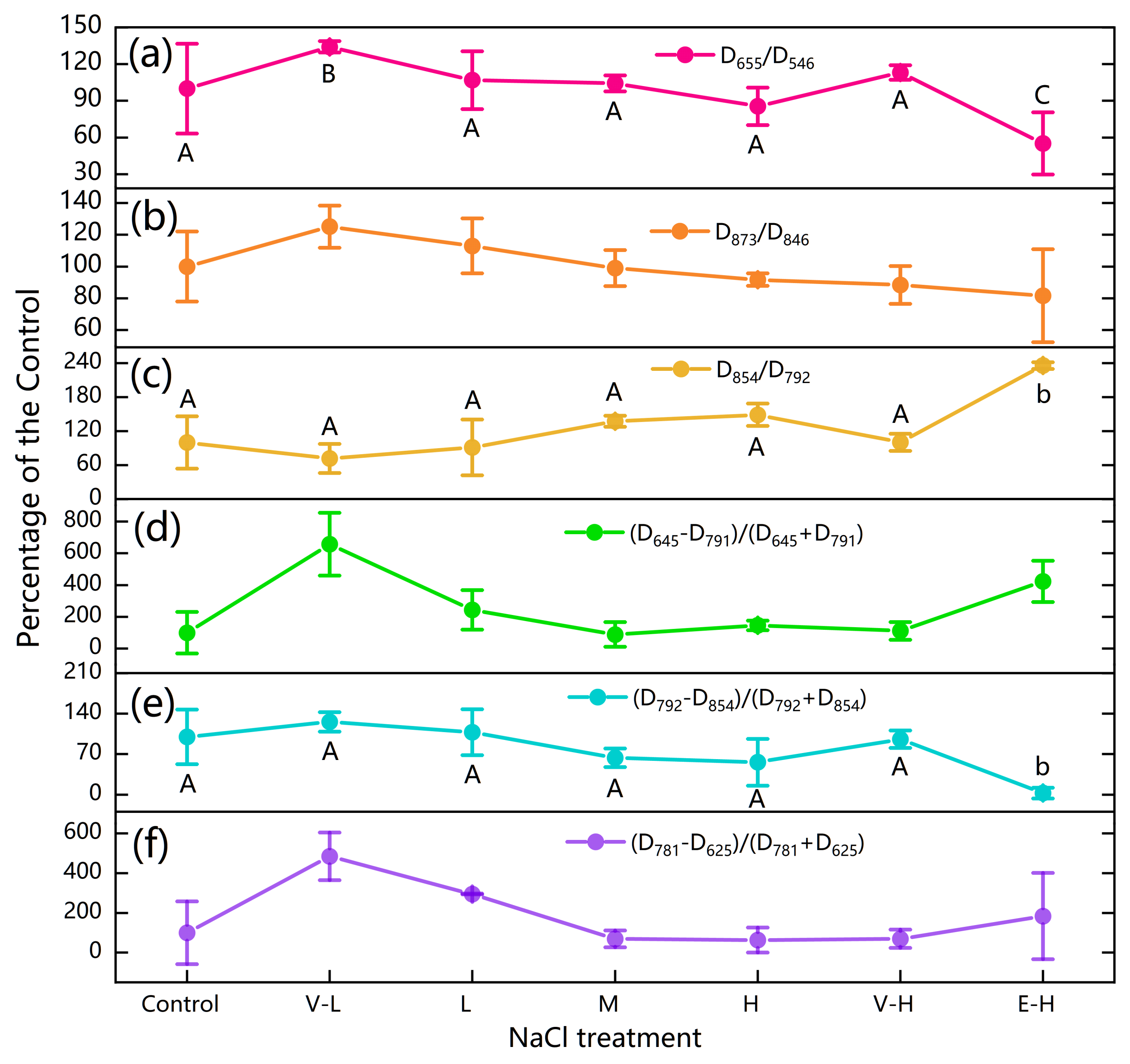
3.3.3. Response of Sensitive Vegetation Indices to Total Chlorophyll Content

There was strong relationship between total chlorophyll content and canopy reflectance changes in Suaeda salsa, caused by different salt conditions. Figure 6 shows the correlation coefficient and significance level matrix between hyperspectral vegetation indices and total chlorophyll content, indicating that vegetation indices D_RVI and D_NDVI from 500 to 900 nm were significantly related to total chlorophyll content (as shown in Figure 6b,d, p < 0.001). Sensitive vegetation indices, such as D_RVI and D_NDVI to total chlorophyll content, were found using the following procedures. D_RVI, D_x was mainly concentrated in the regions of 542–549 nm, 650–659 nm, 848–856 nm, 873 nm, and 897 nm, whereas D_y was primarily focused in the regions of 543–547 nm, 648–661 nm, 786–793 nm, and 845–847 nm (Figure 6a,b). The coefficient a for D_NDVI was mainly concentrated in the regions of 624–626 nm, 639–645 nm, 780–801 nm, 845–857 nm, and 873 nm. The coefficient b was determined from the regions of 624–626 nm, 780–781 nm, 781–793 nm, 791–801 nm, and 845–848 nm (Figure 6c,d). Then, six sensitive vegetation indices (VIs) were retrieved as D₆₅₅/D₅₄₆, D₈₇₃/D_846, D₈₅₄/D₇₉₂, (D₆₄₅ − D₇₉₁)/(D₆₄₅ + D₇₉₁), (D₇₉₂ − D₈₅₄)/(D₇₉₂ + D₈₅₄), and (D₇₈₁ − D₆₂₅)/(D₇₈₁ + D₆₂₅).

Figure 7 shows the ANOVA result between the 6-VIs and salt treatments. Three vegetation indices, i.e., D₆₅₅/D₅₄₆ (F_6,14 = 5.083, p = 0.006), D₈₅₄/D₇₉₂ (F_6,14 = 10.622, p = 0.00012), and (D₇₉₂ − D₈₅₄)/(D₇₉₂ + D₈₅₄) (F_6,14 = 6.74, p = 0.002) significantly differed with salt conditions (p < 0.01) (

Table 5. Optimal VIs under different salt treatments with means ± standard errors (n = 3).

Index	Control	50 mmol/L	100 mmol/L	200 mmol/L	300 mmol/L	400 mmol/L	600 mmol/L
D655/D546	−1.12 ± 0.41	−1.5 ± 0.07	−1.2 ± 0.28	−1.17 ± 0.08	−0.96 ± 0.15	−1.27 ± 0.08	−0.62 ± 0.16
D873/D846	0.94 ± 0.21	1.18 ± 0.16	1.06 ± 0.18	0.93 ± 0.11	0.86 ± 0.03	0.83 ± 0.1	0.77 ± 0.22
D854/D792	0.42 ± 0.19	0.3 ± 0.08	0.38 ± 0.19	0.57 ± 0.06	0.62 ± 0.12	0.42 ± 0.06	0.98 ± 0.06
(D645 − D791)/(D645 + D791)	−5.8 ± 7.6	−38.11 ± 75.07	−14.14 ± 17.65	5.17 ± 4	8.5 ± 2.56	6.46 ± 3.65	24.56 ± 31.87
(D792 − D854)/(D792 + D854)	0.43 ± 0.2	0.54 ± 0.09	0.47 ± 0.18	0.28 ± 0.04	0.24 ± 0.1	0.41 ± 0.06	0.01 ± 0.03
(D781 − D625)/(D781 + D625)	6.55 ± 10.39	31.76 ± 38.2	−19.35 ± 0.35	−4.54 ± 1.92	−4.19 ± 2.63	−4.59 ± 2.11	−12.06 ± 26.17

and Figure 7). Two vegetation indices, D₆₅₅/D₅₄₆ and D₈₅₄/D₇₉₂, for the E-H treatment were lower than for the control, whereas D₆₅₅/D₅₄₆ for the V-L treatment was higher than for the control (p <0.01).

Vegetation indices D₆₅₅/D_546, D₈₅₄/D₇₉₂, and (D₇₉₂ − D₈₅₄)/(D₇₉₂ + D₈₅₄) of Suaeda salsa were used to estimate the total chlorophyll content among all salt treatments using a quadratic polynomial model, with R² = 0.97 (p = 0.000876), R² = 0.966 (p = 0.0011), and R² = 0.96 (p = 0.0013), respectively (Figure 9a,c,e).

4. Discussion

4.1. Effects on Plant Parameters of Suaeda Salsa

Soil salinity is a major abiotic stressor that negatively affects plant growth and ecosystem health in coastal wetlands [43]. Leaf succulence allows Suaeda salsa to adapt to saline environments, with parenchyma cells multiplying so that volume also increases, allowing the plant to absorb and store large quantities of water. As a result, the water content in the unit volume of tissue increases, diluting the salt that the plant absorbs from the soil and maintaining its normal physiological activities [44,45,46,47].

Our study demonstrated that compared with the control, the FW, root length, branching number, and height of Suaeda salsa clearly increased with increasing salt treatments ranging from V-L to M, peaking with the M treatment. However, these parameters decreased slightly with further increased salt treatments ranging from M to E-H (Figure 3a–c). These results are consistent with those of many previous studies [48,49,50]. Our results suggest that a salt concentration of around 200 mmol/L (11.688 g/kg) is optimal for growth of Suaeda salsa. This finding is consistent with the field survey situation and very closely resembles salt soil concentrations of 207 mmol/L, which are suitable for growth of Suaeda salsa [51]. When salt concentrations in the soil exceed 275 mmol/L, the growth of Suaeda salsa is inhibited [52]. The leaf succulence of Suaeda salsa reached its peak value with the M salt treatment, perhaps because Suaeda salsa increased the thickness of thin-walled tissue cells, expanded in volume, and increased leaf succulence level to absorb additional water with which to dilute salt concentrations, maintaining its growth; this is potentially the reason why the morphological indicators of Suaeda salsa peaked at a ~200 mmol/L salt concentration in our study; however, excessively high salt concentrations will obviously weaken this phenomenon [53,54,55].

Changes in chlorophyll content are among the most important physiological indicators for monitoring plant stress. The response of the chlorophyll content to plant stress is closely related [56,57,58]. In our study, it was found that the chlorophyll and carotenoid contents gradually decreased with increasing salt concentrations (from V-L to H), and reached the highest values for the V-L treatment (Figure 3d). This suggests that an appropriate salt concentration in the soil can improve the growth of Suaeda salsa. Our result is similar to that of Guan [10], who determined that the contents of chlorophyll a, b, total chlorophyll, and carotenoid decreased significantly with increasing soil salinity and water table levels.

Figure 3 shows that the response characteristics of physiological indicators were different from those of the other morphological indicators of Suaeda salsa, such as root length and FW. This could be explained by the fact that the chloroplast and mitochondria of Suaeda salsa would first be damaged by sodium ions and then form reactive oxygen species (ROS) with increasing salt concentrations [59]. The antioxidant response system (ARS) in plant cells reached a balance by removing ROS to protect cells from oxidative damage [60]. However, high salt concentrations (>200 mmol/L) will break this balance and inhibit the growth of Suaeda salsa. It also indirectly indicates that this salt-tolerant plant can grow normally with a salt concentration of 50–200mmol/L. Thus, a Suaeda salsa community could ameliorate soil salinization in degraded coastal wetlands.

4.2. Mechanisms and Potential for Monitoring Plant Stress Using Red Edge and Sensitive Vegetation Indices

An ANOVA of the red edge parameters and salt treatment found that the responses of the former to the different salt conditions were not ideal (Table 4 and Figure 5). Only red edge area and amplitude significantly differed with salt treatment. This result was also supported by scatter plots and fitting trendlines of red edge parameters and chlorophyll content, as shown in Figure 8, with only red edge amplitude having a relatively good-fitting trend (RMSE = 0.521). Our results differed from those of many previous studies that used the red edge parameters of vegetation to monitor changes to vegetation under salt stress [61,62], perhaps reflecting the various responses of the red edge parameters for different plant types and stressors. It is also possible that red edge parameters are suitable for detecting plant biophysical and biochemical parameters. Zhu et al., for example, used red edge area and slope to monitor plant response to phenanthrene [26].

This study also found that the optimal wavelengths (x, y, a, and b in Equations (5) and (6)) to compute D_RVI and D_NDVI were mainly concentrated between 786–793 nm and 848–856 nm (Figure 6). An analysis of the response of sensitive vegetation indices D₈₅₄/D₇₉₂ and (D₇₉₂ − D₈₅₄)/(D₇₉₂ + D₈₅₄) to salt treatment supports this finding (Figure 8, Figure 9, and Figure 10). However, no valid band combinations were found in the red edge range (i.e., 680–750 nm). This finding differed from that of some scholars, who used the red edge band to construct vegetation indices to estimate total chlorophyll content [39,63]. On the other hand, some others have reported that vegetation indices constructed in the near-infrared band were highly correlated with total chlorophyll content [64,65]. Although the vegetation indices constructed in the near-infrared band were highly accurate for the inversion of chlorophyll content [66,67] in the salt treatment in our study, this needs to be further refined in the future study.

In the present study, vegetation indices D_RVI and D_NDVI were more suitable for than the red edge parameters of Suaeda salsa for estimating the total chlorophyll content under different salt conditions (Figure 7). In particular, the three vegetation indices, D₆₅₅/D₅₄₆, D₈₅₄/D₇₉₂, and (D₇₉₂ − D₈₅₄)/(D₇₉₂ + D₈₅₄), effectively simulated total chlorophyll content (Figure 9). Figure 10 shows that two vegetation indices, D₈₅₄/D₇₉₂ and (D₇₉₂ − D₈₅₄)/(D₇₉₂ + D₈₅₄), were sensitive to salt treatment, with indices D_RVI and D_NDVI showing significantly better capacity than the red edge parameters for estimating salt treatments and total chlorophyll content. In addition, vegetation indices that were sensitive to total chlorophyll content showed potential for simulating soil salt concentration. Because changes in soil salt can affect plant growth indicators, influencing vegetation reflectance spectra, vegetation indices show promise for monitoring vegetation response to salt stress; this is perhaps the primary reason why many previous studies have used multiple vegetation indices to monitor vegetation changes [68,69,70] in coastal wetlands.

5. Conclusions

Applying seven different salt concentrations, we analyzed the response of plant growth indicators and canopy reflectance to different salt treatments in coastal wetlands. Taking the Dafeng Elk National Nature Reserve (DENNR) in China as a case study, we collected Suaeda salsa seedlings and divided them into seven groups to conduct potted experiments, using ANOVA analysis to study the responses of plant growth indicators such as height, FW, DW, and chlorophyll content. We assessed the responses of Suaeda salsa canopy reflectance to salt treatment using red edge parameters and sensitive vegetation indices. We also estimated the total chlorophyll content which was most sensitive to salt conditions using red edge parameters and vegetation indices. Our conclusions were as follows:

(1)

Among all physiological indicators, the total chlorophyll content of Suaeda salsa showed the best response to the salt treatment.

(2)

The red edge parameters and vegetation indices that were sensitive to salt treatments were red edge area, red edge amplitude, D₈₅₄/D₇₉₂, and (D₇₉₂ − D₈₅₄)/(D₇₉₂ + D₈₅₄).

(3)

Compared with the red edge parameters, the vegetation indices D_RVI and D_NDVI strongly correlated with total chlorophyll content for the different salt treatments (p <0.01). The vegetation indices constructed based on the first derivative reflectance of the canopy spectra in the near-infrared band combination between 786–793 nm and 848–856 nm correlated best with the chlorophyll content of Suaeda salsa for the different salt treatments, especially for vegetation indices D₈₅₄/D₇₉₂,D₆₅₅/D₅₄₆,and (D₇₉₂ − D₈₅₄)/(D₇₉₂ + D₈₅₄).

Multiple factors, such as groundwater and salinity, may affect the growth and spectral characteristics of Suaeda salsa. In future studies, Suaeda salsa’s mechanism of hyperspectral response to water table and salt stress should be further studied in pot experiments or in the field.

References

1. Taddeo, S.; Dronova, I.; Depsky, N. Spectral vegetation indices of wetland greenness: Responses to vegetation structure, composition, and spatial distribution. Remote Sens. Environ. 2019, 234, 111467. [Google Scholar] [CrossRef]
2. Cui, B.; He, Q.; Zhao, X. Ecological thresholds of Suaeda salsa to the environmental gradients of water table depth and soil salinity. Acta Ecol. Sin. 2008, 28, 1408–1418. [Google Scholar] [CrossRef]
3. Zheng, C.; Jiang, D.; Liu, F.; Dai, T.; Jing, Q.; Cao, W. Effects of salt and waterlogging stresses and their combination on leaf photosynthesis, chloroplast ATP synthesis, and antioxidant capacity in wheat. Plant Sci. 2009, 176, 575–582. [Google Scholar] [CrossRef] [PubMed]
4. Saqib, M.; Akhtar, J.; Qureshi, R.H. Na+ exclusion and salt resistance of wheat (Triticum aestivum) in saline-waterlogged conditions are improved by the development of adventitious nodal roots and cortical root aerenchyma. Plant Sci. 2005, 169, 125–130. [Google Scholar] [CrossRef]
5. Wang, B.; Lüttge, U.; Ratajczak, R. Specific regulation of SOD isoforms by NaCl and osmotic stress in leaves of the C3 halophyte Suaeda salsa L. J. Plant Physiol. 2004, 161, 285–293. [Google Scholar] [CrossRef]
6. Li, J.; Hussain, T.; Feng, X.; Guo, K.; Chen, H.; Yang, C.; Liu, X. Comparative study on the resistance of Suaeda glauca and Suaeda salsa to drought, salt, and alkali stresses. Ecol. Eng. 2019, 140, 105593. [Google Scholar] [CrossRef]
7. An, Y.; Gao, Y.; Zhang, Y.; Tong, S.; Liu, X. Early establishment of Suaeda salsa population as affected by soil moisture and salinity: Implications for pioneer species introduction in saline-sodic wetlands in Songnen Plain, China. Ecol. Indic. 2019, 107, 105654. [Google Scholar] [CrossRef]
8. Li, X.; Zhang, X.; Wang, X.; Yang, X.; Cui, Z. Bioaugmentation-assisted phytoremediation of lead and salinity co-contaminated soil by Suaeda salsa and Trichoderma asperellum. Chemosphere 2019, 224, 716–725. [Google Scholar] [CrossRef]
9. Song, J.; Fan, H.; Zhao, Y.; Jia, Y.; Du, X.; Wang, B. Effect of salinity on germination, seedling emergence, seedling growth and ion accumulation of a euhalophyte Suaeda salsa in an intertidal zone and on saline inland. Aquat. Bot. 2008, 88, 331–337. [Google Scholar] [CrossRef]
10. Guan, B.; Yu, J.; Wang, X.; Fu, Y.; Kan, X.; Lin, Q.; Han, G.; Lu, Z. Physiological Responses of Halophyte Suaeda salsa to Water Table and Salt Stresses in Coastal Wetland of Yellow River Delta. Clean Soil Air Water. 2011, 39, 1029–1035. [Google Scholar] [CrossRef]
11. Bueno, M.; Lendínez, M.L.; Calero, J.; Del Pilar Cordovilla, M. Salinity responses of three halophytes from inland saltmarshes of Jaén (Southern Spain). Flora. Morphol. Geobotanik Oekophysiol. 2020, 266, 151589. [Google Scholar] [CrossRef]
12. Ferreira, J.F.S.; Liu, X.; Suarez, D.L. Fruit yield and survival of five commercial strawberry cultivars under field cultivation and salinity stress. Sci. Hortic. Amsterdam 2019, 243, 401–410. [Google Scholar] [CrossRef]
13. Chen, B.; Sun, Z. Effects of nitrogen enrichment on variations of sulfur in plant-soil system of Suaeda salsa in coastal marsh of the Yellow River estuary, China. Ecol. Indic. 2020, 109, 105797. [Google Scholar] [CrossRef]
14. Zhang, S.; Bai, J.; Wang, W.; Huang, L.; Zhang, G.; Wang, D. Heavy metal contents and transfer capacities of Phragmites australis and Suaeda salsa in the Yellow River Delta, China. Phys. Chem. Earth Parts A B C 2018, 104, 3–8. [Google Scholar] [CrossRef]
15. Sun, Z.; Mou, X.; Zhang, D.; Sun, W.; Hu, X.; Tian, L. Impacts of burial by sediment on decomposition and heavy metal concentrations of Suaeda salsa in intertidal zone of the Yellow River estuary, China. Mar. Pollut. Bull. 2017, 116, 103–112. [Google Scholar] [CrossRef]
16. Mou, X.J.; Sun, Z.G. Effects of sediment burial disturbance on seedling emergence and growth of Suaeda salsa in the tidal wetlands of the Yellow River estuary. J. Exp. Mar. Biol. Ecol. 2011, 409, 99–106. [Google Scholar] [CrossRef]
17. Liu, P.; Wang, Q.; Bai, J.; Gao, H.; Huang, L.; Xiao, R. Decomposition and return of C and N of plant litters of Phragmites australis and Suaeda salsa in typical wetlands of the Yellow River Delta, China. Proc. Environ. Sci. 2010, 2, 1717–1726. [Google Scholar] [CrossRef] [Green Version]
18. Zhang, G.S.; Wang, R.Q.; Song, B.M. Plant community succession in modern Yellow River Delta, China. J. Zhejiang Univ. Sci. B 2007, 8, 540–548. [Google Scholar] [CrossRef] [Green Version]
19. Alexander, F.H.G.; Vane, G.; Solomon, J.E.; Rock, B.N. Imaging Spectrometry for Earth Remote Sensing. Science 1985, 228, 1147–1153. [Google Scholar] [CrossRef]
20. Yi, Q.; Huang, J.; Wang, F.; Wang, X.; Liu, Z. Monitoring Rice Nitrogen Status Using Hyperspectral Reflectance and Artificial Neural Network. Environ. Sci. Technol. 2007, 41, 6770–6775. [Google Scholar] [CrossRef]
21. Zhang, H.; Hu, H.; Zhang, X.; Wang, K.; Song, T.; Zeng, F. Detecting Suaeda salsa L. chlorophyll fluorescence response to salinity stress by using hyperspectral reflectance. Acta Physiol. Plant. 2012, 34, 581–588. [Google Scholar] [CrossRef]
22. Li, G.; Wan, S.; Zhou, J.; Yang, Z.; Qin, P. Leaf chlorophyll fluorescence, hyperspectral reflectance, pigments content, malondialdehyde and proline accumulation responses of castor bean (Ricinus communis L.) seedlings to salt stress levels. Ind. Crop. Prod. 2010, 31, 13–19. [Google Scholar] [CrossRef]
23. Obermeier, W.A.; Lehnert, L.W.; Pohl, M.J.; Makowski Gianonni, S.; Silva, B.; Seibert, R.; Laser, H.; Moser, G.; Müller, C.; Luterbacher, J.; et al. Grassland ecosystem services in a changing environment: The potential of hyperspectral monitoring. Remote Sens. Environ. 2019, 232, 111273. [Google Scholar] [CrossRef]
24. Ren, G.; Zhang, J.; Ma, Y. Spectral discrimination and separable feature lookup table of typical vegetation species in Yellow River Delta wetland. Mar. Environ. Sci. 2015, 34, 420–426. [Google Scholar]
25. Wu, T.; Zhao, D.; Kang, J.; Suo, A.; Wei, B.; Ma, Y. Research on remote sensing inversion biomass method based on the Suaeda Salsa’ s measured spectrum. Spectrosc. Spect. Anal. 2010, 30, 1336–1341. [Google Scholar] [CrossRef]
26. Zhu, L.; Chen, Z.; Wang, J.; Ding, J.; Yu, Y.; Li, J.; Xiao, N.; Jiang, L.; Zheng, Y.; Rimmington, G.M. Monitoring plant response to phenanthrene using the red edge of canopy hyperspectral reflectance. Mar. Pollut. Bull. 2014, 86, 332–341. [Google Scholar] [CrossRef]
27. González-Piqueras, J.; Lopez-Corcoles, H.; Sánchez, S.; Villodre, J.; Bodas, V.; Campos, I.; Osann, A.; Calera, A. Monitoring crop N status by using red edge-based indices. Adv. Anim. Biosci. 2017, 8, 338–342. [Google Scholar] [CrossRef]
28. Kanke, Y.; Tubaña, B.; Dalen, M.; Harrell, D. Evaluation of red and red-edge reflectance-based vegetation indices for rice biomass and grain yield prediction models in paddy fields. Precis. Agric. 2016, 17, 507–530. [Google Scholar] [CrossRef]
29. Ali, A.; Imran, M.M. Evaluating the potential of red edge position (REP) of hyperspectral remote sensing data for real time estimation of LAI & chlorophyll content of kinnow mandarin (Citrus reticulata) fruit orchards. Sci. Hortic. 2020, 267, 109326. [Google Scholar] [CrossRef]
30. Li, L.; Ren, T.; Ma, Y.; Wei, Q.; Wang, S.; Li, X.; Cong, R.; Liu, S.; Lu, J. Evaluating chlorophyll density in winter oilseed rape (Brassica napus L.) using canopy hyperspectral red-edge parameters. Comput. Electron. Agric. 2016, 126, 21–31. [Google Scholar] [CrossRef]
31. Filella, I.; Penuelas, J. The red edge position and shape as indicators of plant chlorophyll content, biomass and hydric status. Int. J. Remote Sens. 1994, 15, 1459–1470. [Google Scholar] [CrossRef]
32. Yao, F.; Zhang, Z.; Yang, R.; Sun, J.; Cui, S. Hyperspectral models for estimating vegetation chlorophyll content based on red edge parameter. Trans. Chin. Soc. Agric. Eng. 2009, 25, 123–129. [Google Scholar]
33. Xue, J.; Su, B. Significant Remote Sensing Vegetation Indices: A Review of Developments and Applications. J. Sens. 2017, 2017, 1–17. [Google Scholar] [CrossRef] [Green Version]
34. Kross, A.; McNairn, H.; Lapen, D.; Sunohara, M.; Champagne, C. Assessment of RapidEye vegetation indices for estimation of leaf area index and biomass in corn and soybean crops. Int. J. Appl. Earth Obs. 2015, 34, 235–248. [Google Scholar] [CrossRef] [Green Version]
35. Lu, X.; Wang, X.; Sun, H.; Yu, Y.; Wang, Y.; Yang, J.; Zhang, L. The estimation model of biomass of Suaeda Salsa in coastal wetland based on hyperspectral reflectance spectra. Trans. Oceanol. Limnol. 2017, 2, 96–100. [Google Scholar]
36. Zhao, X.; Ling, Y.; Zhang, G.; Jie, S.; Hua, W.; Ding, Y. Community characteristics of beach wetland vegetations along a habitat gradient in Dafeng Milu Reserve of Jiangsu Province. Chin. J. Ecol. 2010, 29, 244–249. [Google Scholar]
37. Zhao, S.; Shi, G.; Dong, X. The Guidance of Plant Physiology Experiments; Agricultural Science and Technology Press: Beijing, China, 2002. [Google Scholar]
38. Jiang, C.; Chen, Y.; Wu, H.; Li, W.; Zhou, H.; Bo, Y.; Shao, H.; Song, S.; Puttonen, E.; Hyyppä, J. Study of a High Spectral Resolution Hyperspectral LiDAR in Vegetation Red Edge Parameters Extraction. Remote Sens. 2019, 11, 2007. [Google Scholar] [CrossRef] [Green Version]
39. Ju, C.; Tian, Y.; Yao, X.; Cao, W.; Zhu, Y.; Hannaway, D. Estimating Leaf Chlorophyll Content Using Red Edge Parameters. Pedosphere 2010, 20, 633–644. [Google Scholar] [CrossRef]
40. Zhao, D.; Huang, L.; Li, J.; Qi, J. A comparative analysis of broadband and narrowband derived vegetation indices in predicting LAI and CCD of a cotton canopy. ISPRS J. Photogramm. 2007, 62, 25–33. [Google Scholar] [CrossRef]
41. Broge, N.H.; Leblanc, E. Comparing prediction power and stability of broadband and hyperspectral vegetation indices for estimation of green leaf area index and canopy chlorophyll density. Remote Sens. Environ. 2001, 76, 156–172. [Google Scholar] [CrossRef]
42. Inoue, Y.; Guérif, M.; Baret, F.; Skidmore, A.; Gitelson, A.; Schlerf, M.; Darvishzadeh, R.; Olioso, A. Simple and robust methods for remote sensing of canopy chlorophyll content: A comparative analysis of hyperspectral data for different types of vegetation. Plant Cell Environ. 2016, 39, 2609–2623. [Google Scholar] [CrossRef] [PubMed] [Green Version]
43. Carter, G.A. Responses of leaf spectral reflectance to plant stress. Am. J. Bot. 1993, 80, 239–243. [Google Scholar] [CrossRef]
44. Kefu, Z.; Hai, F.; San, Z.; Jie, S. Study on the salt and drought tolerance of Suaeda salsa and Kalanchoe claigremontiana under iso-osmotic salt and water stress. Plant Sci. 2003, 165, 837–844. [Google Scholar] [CrossRef]
45. Jennings, D.H. Halophytes, Succulence and Sodium in Plants-A Unified Theory. New Phytologist. 1968, 67, 899–911. [Google Scholar] [CrossRef]
46. Eshel, A. Response of Suaeda aegyptiaca to KCl, NaCl and Na2SO4 treatments. Physiol. Plantarum. 1985, 64, 308–315. [Google Scholar] [CrossRef]
47. Ajmal Khan, M.; Ungar, I.A.; Showalter, A.M. The effect of salinity on the growth, water status, and ion content of a leaf succulent perennial halophyte, Suaeda fruticosa (L.) Forssk. J. Arid Environ. 2000, 45, 73–84. [Google Scholar] [CrossRef] [Green Version]
48. Jia, J.; Huang, C.; Bai, J.; Zhang, G.; Zhao, Q.; Wen, X. Effects of drought and salt stresses on growth characteristics of euhalophyte Suaeda salsa in coastal wetlands. Phys. Chem. Earth Parts A B C 2018, 103, 68–74. [Google Scholar] [CrossRef]
49. Song, J.; Shi, G.; Gao, B.; Fan, H.; Wang, B. Waterlogging and salinity effects on two Suaeda salsa populations. Physiol. Plantarum. 2011, 141, 343–351. [Google Scholar] [CrossRef]
50. Lu, Q.; Lu, C.; Qiu, N.; Wang, B.; Kuang, T. Does salt stress lead to increased susceptibility of photosystem II to photoinhibition and changes in photosynthetic pigment composition in halophyte Suaeda salsa grown outdoors? Plant Sci. 2002, 163, 1063–1068. [Google Scholar] [CrossRef]
51. Wang, B.; Han, J.; Zhou, Z.; Dong, Y.; Guan, X.; Jiang, B. Ecological thresholds of Suadea heteroptera under gradients of soil salinity and moisture in Daling River estuarine wetland. Chin. J. Ecol. 2014, 33, 71–75. [Google Scholar] [CrossRef]
52. Li, Y.; Chen, Z.; Wang, J.; Xu, S.; Hou, W. Effects of salt stress on Suaeda heteroptera Kitagawa growth and osmosis-regulating substance concentration. Chin. J. Ecol. 2011, 30, 72–76. [Google Scholar]
53. Qi, C.; Chen, M.; Song, J.; Wang, B. Increase in aquaporin activity is involved in leaf succulence of the euhalophyte Suaeda salsa, under salinity. Plant Sci. 2009, 176, 200–205. [Google Scholar] [CrossRef]
54. Cai Hong, P.; Su Jun, Z.; Zhi Zhong, G.; Bao Shan, W. NaCl treatment markedly enhances H2O2—Scavenging system in leaves of halophyte Suaeda salsa. Physiol. Plantarum 2005, 125, 490–499. [Google Scholar] [CrossRef]
55. Liu, X.; Duan, D.; Li, W.; Tadano, T. A Comparative Study on Responses of Growth and Solute Composition in Halophytes Suaeda Salsa and Limonium Bicolor to Salinity; Springer: Dordrecht, The Netherlands, 2008; Volume 40, pp. 135–143. [Google Scholar]
56. Gitelson, A.A.; Merzlyak, M.N. Non-destructive assessment of chlorophyll carotenoid and anthocyanin content in higher plant leaves: Principles and algorithms. Remote Sens. Agric. Environ. 2004, 263, 78–94. [Google Scholar]
57. Lobos, G.A.; Retamales, J.B.; Hancock, J.F.; Flore, J.A.; Cobo, N.; Del Pozo, A. Spectral irradiance, gas exchange characteristics and leaf traits of Vaccinium corymbosum L. ‘Elliott’ grown under photo-selective nets. Environ. Exp. Bot. 2012, 75, 142–149. [Google Scholar] [CrossRef]
58. Garriga, M.; Retamales, J.B.; Romero-Bravo, S.; Caligari, P.D.; Lobos, G.A. Chlorophyll, anthocyanin, and gas exchange changes assessed by spectroradiometry in Fragaria chiloensis under salt stress. J. Integr. Plant Biol. 2014, 56, 505–515. [Google Scholar] [CrossRef]
59. Hernández, J.A.; Olmos, E.; Corpas, F.J.; Sevilla, F.; Del Río, L.A. Salt-induced oxidative stress in chloroplasts of pea plants. Plant Sci. 1995, 105, 151–167. [Google Scholar] [CrossRef]
60. Asada, K. The water-water cycle in chloroplasts: Scavenging of active oxygens and dissipation of excess photons. Annu. Rev. Plant Physiol. Plant Mol. Biol. 1999, 50, 601–639. [Google Scholar] [CrossRef]
61. Liu, L.; Wang, J.; Huang, W.; Zhao, C.; Zhang, B.; Tong, Q. Estimating winter wheat plant water content using red edge parameters. Int. J. Remote Sens. 2004, 25, 3331–3342. [Google Scholar] [CrossRef]
62. Zheng, J.; Li, F.; Du, X. Using Red Edge Position Shift to Monitor Grassland Grazing Intensity in Inner Mongolia. J. Indian Soc. Remote 2018, 46, 81–88. [Google Scholar] [CrossRef]
63. Fitzgerald, G.; Rodriguez, D.; O’Leary, G. Measuring and predicting canopy nitrogen nutrition in wheat using a spectral index—The canopy chlorophyll content index (CCCI). Field Crop. Res. 2010, 116, 318–324. [Google Scholar] [CrossRef]
64. Zhang, T.; Zeng, S.; Gao, Y.; Ouyang, Z.; Li, B.; Fang, C.; Zhao, B. Using hyperspectral vegetation indices as a proxy to monitor soil salinity. Ecol. Indic. 2011, 11, 1552–1562. [Google Scholar] [CrossRef]
65. Ji, C.; Zhang, Y.; Cheng, Q.; Li, Y.; Jiang, T.; San Liang, X. Analyzing the variation of the precipitation of coastal areas of eastern China and its association with sea surface temperature (SST) of other seas. Atmos. Res. 2019, 219, 114–122. [Google Scholar] [CrossRef]
66. Zhang, Y.; Huang, Z.; Fu, D.; Tsou, J.Y.; Jiang, T.; Liang, X.S.; Lu, X. Monitoring of chlorophyll-a and sea surface silicate concentrations in the south part of Cheju island in the East China sea using MODIS data. Int. J. Appl. Earth Obs. 2018, 67, 173–178. [Google Scholar] [CrossRef]
67. Ji, C.; Zhang, Y.; Cheng, Q.; Tsou, J.; Jiang, T.; Liang, X.S. Evaluating the impact of sea surface temperature (SST) on spatial distribution of chlorophyll-a concentration in the East China Sea. Int. J. Appl. Earth Obs. 2018, 68, 252–261. [Google Scholar] [CrossRef]
68. Souza, A.A.; Galvão, L.S.; Santos, J.R. Relationships between Hyperion-derived vegetation indices, biophysical parameters, and elevation data in a Brazilian savannah environment. Remote Sens. Lett. 2010, 1, 55–64. [Google Scholar] [CrossRef]
69. Peng, Y.; Gitelson, A.A. Application of chlorophyll-related vegetation indices for remote estimation of maize productivity. Agric. For. Meteorol. 2011, 151, 1267–1276. [Google Scholar] [CrossRef]
70. Kooistra, L.; Clevers, J.G.P.W. Estimating potato leaf chlorophyll content using ratio vegetation indices. Remote Sens. Lett. 2016, 7, 611–620. [Google Scholar] [CrossRef] [Green Version]
Figure 1. The study area at the Dafeng Elk National Nature Reserve in China.
Remotesensing 12 02700 g001
Figure 2. Photographs of potted plants of Suaeda salsa under salt stress in seven groups (taken on the last day of the experiment). Each group of experiments consisted of three pots of samples, in which photos (AC) are the Control group, (DF) are the V-L group, (GI) are the L group, and (JL) are the M group, (MO) are the H group, (PR) are the V-H group, and (SU) are the E-H group.
Remotesensing 12 02700 g002
Figure 3. Effects of different salt concentration stress on various physiological indexes of Suaeda salsa. The control group was set to 100%, and the remaining six groups were changed relative to the control group. The values were means ± standard errors (n = 3). The real values are presented in Table 3. ((a) plant height, root length, number of branches; (b) leaf succulence, FW above the ground, DW above the ground; (c) FW of root, DW of root; (d) chlorophyll a, chlorophyll b, total chlorophyll contents and carotenoid content of Suaeda salsa).
Remotesensing 12 02700 g003
Figure 4. The original spectral curve (a) and the first derivative spectral curve (b) under different stresses with different salt concentrations.
Remotesensing 12 02700 g004
Figure 5. Trend of red edge area (a), skewness (b), kurtosis (c), amplitude (d) and position (e) of Suaeda salsa under different NaCl treatments. The control group was set to 100%, and the remaining six groups were changed relative to the control group. The values were means ± standard errors (n = 3). The real values are presented in Table 4. Capital and lower-case letters above the bars indicate significant differences at the levels of 0.05 and 0.01. If no letter is assigned above the band, it means that this item is not significant to salt stress (p > 0.05). Other descriptions are as in Figure 3.
Remotesensing 12 02700 g005
Figure 6. The correlation coefficient matrix (a) and significance level matrix (b) between the ratio vegetation indices based on derivative reflectance (D_RVI) and total chlorophyll content, and the correlation coefficient matrix (c) and significance level matrix (d) of normalized difference vegetation indices (NDVI) based on derivative reflectance (D_NDVI) and total chlorophyll content. The red regions indicate the significance level p < 0.001.
Remotesensing 12 02700 g006
Figure 7. Changes in the sensitive vegetation indices D655/D546 (a), D873/D846 (b), D854/D792 (c), (D645 − D791)/(D645 + D791) (d), (D792 − D854)/(D792 + D854) (e) and (D781 − D625)/(D781 + D625) (f) of Suaeda salsa under different NaCl treatments. The control group was set to 100%, and the remaining six groups were changed relative to the control. The values were means ± standard errors (n = 3). Capital and lower-case letters above the bars indicate significant differences at the levels of 0.05 and 0.01. If no letter is assigned above the bars, it means that this item was not significant to salt treatments (p > 0.05). The real values are presented in Table 5. Other descriptions are as in Figure 3.
Remotesensing 12 02700 g007
Figure 8. Relationship between total chlorophyll content of Suaeda salsa and measured red edge area (a), amplitude (b), skewness (c), kurtosis (d), position (e). The error bars represent the standard error of the mean of the chlorophyll and various red edge parameters (n = 3). The red curve represents a quadratic polynomial fit.
Remotesensing 12 02700 g008
Figure 9. The relationship between the chlorophyll content of Suaeda salsa and the best vegetation indices D655/D546 (a), D873/D846 (b), D854/D792 (c), (D645 − D791)/(D645 + D791) (d), (D792 − D854)/(D792 + D854) (e) and (D781 − D625)/(D781 + D625) (f). The error bars represent the standard error of the mean of total chlorophyll content and various red edge parameters (n = 3). The red curve represents a quadratic polynomial fit.
Remotesensing 12 02700 g009
Figure 10. Relationship between applied salt concentration and red edge amplitude (a) and optimal vegetation indices D655/D546 (b), D854/D792 (c) and (D792 − D854)/(D792 + D854) (d). Error bars represent the standard error of the red edge amplitude and the average of the best vegetation indices (n = 3). The red curve represents the best fit line.
Remotesensing 12 02700 g010