UAV-Borne LiDAR Crop Point Cloud Enhancement Using Grasshopper Optimization and Point Cloud Up-Sampling Network

Abstract

Because of low accuracy and density of crop point clouds obtained by the Unmanned Aerial Vehicle (UAV)-borne Light Detection and Ranging (LiDAR) scanning system of UAV, an integrated navigation and positioning optimization method based on the grasshopper optimization algorithm (GOA) and a point cloud density enhancement method were proposed. Firstly, a global positioning system (GPS)/inertial navigation system (INS) integrated navigation and positioning information fusion method based on a Kalman filter was constructed. Then, the GOA was employed to find the optimal solution by iterating the system noise variance matrix Q and measurement noise variance matrix R of Kalman filter. By feeding the optimal solution into the Kalman filter, the error variances of longitude were reduced to 0.00046 from 0.0091, and the error variances of latitude were reduced to 0.00034 from 0.0047. Based on the integrated navigation, an UAV-borne LiDAR scanning system was built for obtaining the crop point. During offline processing, the crop point cloud was filtered and transformed into WGS-84, the density clustering algorithm improved by the particle swarm optimization (PSO) algorithm was employed to the clustering segment. After the clustering segment, the pre-trained Point Cloud Up-Sampling Network (PU-net) was used for density enhancement of point cloud data and to carry out three-dimensional reconstruction. The features of the crop point cloud were kept under the processing of reconstruction model; meanwhile, the density of the crop point cloud was quadrupled.

1. Introduction

Light Detection and Ranging (LiDAR) is an active sensing technology that can quickly acquire spatial information of a target or environment [1,2]. Compared with traditional remote sensing methods, LiDAR has shown great advantages in accuracy and stability [3]. In agriculture, the LiDAR system is one of the most accurate methods to measure regional vegetation structural characteristics and biophysical parameters [4]. The Unmanned Aerial Vehicle (UAV)-borne LiDAR scanning system is one of the most common platforms for crop point cloud obtaining. The crop point clouds captured by UAV-borne LiDAR scanning system are sparse and unordered [5]. The navigation and positioning accuracy of the UAV-borne LiDAR scanning system influences the accuracy of the point cloud data greatly. Density is also an important indicator to measure the quality of point cloud data. Higher point cloud density represents richer information of the target or environment [6]. Ensuring the accuracy and density characteristics of the UAV-borne LiDAR point cloud data while maintaining the cost is crucial for the continuous and efficient execution of LiDAR detection tasks.

For integrated navigation, the most widely used in the world is the global positioning system (GPS)/inertial navigation system (INS) integrated navigation positioning system [7]. The Kalman filter is the most common method of data fusion [8]. Gao et al. [9] developed an INS/GPS/LiDAR integrated navigation system through an extended Kalman filter (EKF) using a hybrid scan matching algorithm. Shabani et al. [10] explored the characteristics, advantages, and disadvantages of direct Kalman filtering and indirect Kalman filtering commonly used in GPS/INS integrated navigation, and a novel asynchronous direct Kalman filter was proposed. Zhang et al. [11] developed a low-cost global navigation satellite system (GNSS) and INS integrated navigation method and an adaptive Kalman filter for overcoming the measurement noise of GNSS, which was proposed based on a supervised machine learning model. Yu et al. [12] used a single-frequency real-time kinematic carrier phase (RTK) technology to deduce and obtain information including speed and orientation under GPS/BeiDou Navigation Satellite System (BDS) for polishing the inaccurate INS information. Norouz et al. [13] proposed an improved Kalman filter algorithm based on small probability distribution of the state variable between the measurement updates of the multi-rate GPS/INS-coupled navigation filter, which greatly reduced the amount of calculation, and the algorithm performed well by numerically simulating. All of the above integrated navigation systems suffered from the low accuracy of integrated navigation, except Yu et al. [12]. However, RTK-based high accuracy integrated navigation systems cannot be widely popularized due to the price gap. During the experiments of data fusion using the Kalman filter, the longitude and latitude errors were sharply affected by the parameter of the Kalman filter, especially system noise sequence Q and measurement noise sequence R, and the same situation also occurred in the realization of Ref. [10,11]. For promoting the accuracy of our integrated navigation-based scanning system, the meta-heuristic method was employed for finding the optimum parameters of integrated navigation in our UAV scanning system. For multi-solution problems, genetic algorithms (GA) [14], particle swarm optimization (PSO) [15], and ant colony optimization (ACO) [16] were the most popular, with swarm intelligence optimization proposed recently such as the bat algorithm (BA) [17] and grasshopper optimization algorithm (GOA) [18]. All of the multi-solution meta-heuristic methods have their own merits for different problems [19]. In order to reduce longitude and latitude errors of integrated navigation, the meta-heuristic methods were employed to find the optimum system noise sequence Q and measurement noise sequence R.

After obtaining the crop point cloud data by UAV scanning system, the raw point cloud data consisted of crop points and other points, and manual classification was extremely inefficient for different point cloud data. Therefore, the clustering segmentation method was employed to extract crop data from raw point cloud data. The density-based clustering method, density-based spatial clustering of applications with noise (DBSCAN), has attracted a lot of attention; besides the improvement of the algorithm itself, finding out the key parameters of clustering was also a new direction of optimization [20]. The same as integrated navigation, the meta-heuristic method was employed to optimize the clustering segmentation method. According to the experimental results of the density distribution characteristics of the plane point cloud under different conditions, Kedzierski et al. [21] found that the point cloud density could be preliminarily estimated based on distance and angle, but the actual point cloud density should take into account the influence of object shape and environment. Rupink et al. [22] proposed the formula and calculation steps for calculating the point cloud density. Huang et al. [23] proposed an edge-sensing point set resampling method, gradually approaching the edges and corners. However, the quality of the results largely depends on the accuracy of the normal of a given point and the fine-tuning of parameters. Based on Ref. [21,23], dense and accurate point clouds are very useful for crop point cloud recognition and 3D reconstruction. The high-cost multi-line LiDAR can be simulated by low-cost single-line LiDAR point clouds through the point cloud up-sampling method without destroying the features.

In view of the current problems and inspired by existing methods, in order to improve the quality of point cloud data, a combined navigation optimization algorithm based on GOA and a point cloud density enhancement algorithm based on Point Cloud Up-Sampling Network (PU-net) were proposed. The novel contribution of this article was as follows:

(1)

In order to obtain the optimal solution of the initial parameters of the Kalman filter quickly and accurately, GOA took the sum of the longitude and latitude error variances as the fitness function to find the optimal solution to iterate the system noise variance matrix Q and the measurement noise variance matrix R. Based on the Q and R matrices from GOA, the positioning error of the UAV-borne LiDAR scanning system was greatly reduced; meanwhile, the computing burden was decreased, and the accuracy of point cloud data acquisition was improved;

(2)

The density clustering algorithm was improved by the linear decreasing particle swarm optimization (PSO) algorithm. In order to solve the problem of sparse density, in this paper, a pre-trained PU-net was used for enhancing the point cloud density of the point cloud data obtained by UAV-borne LiDAR. Experiments have verified that the enhanced point cloud data retain the features of the raw point cloud data.

2. Framework of the Proposed Method

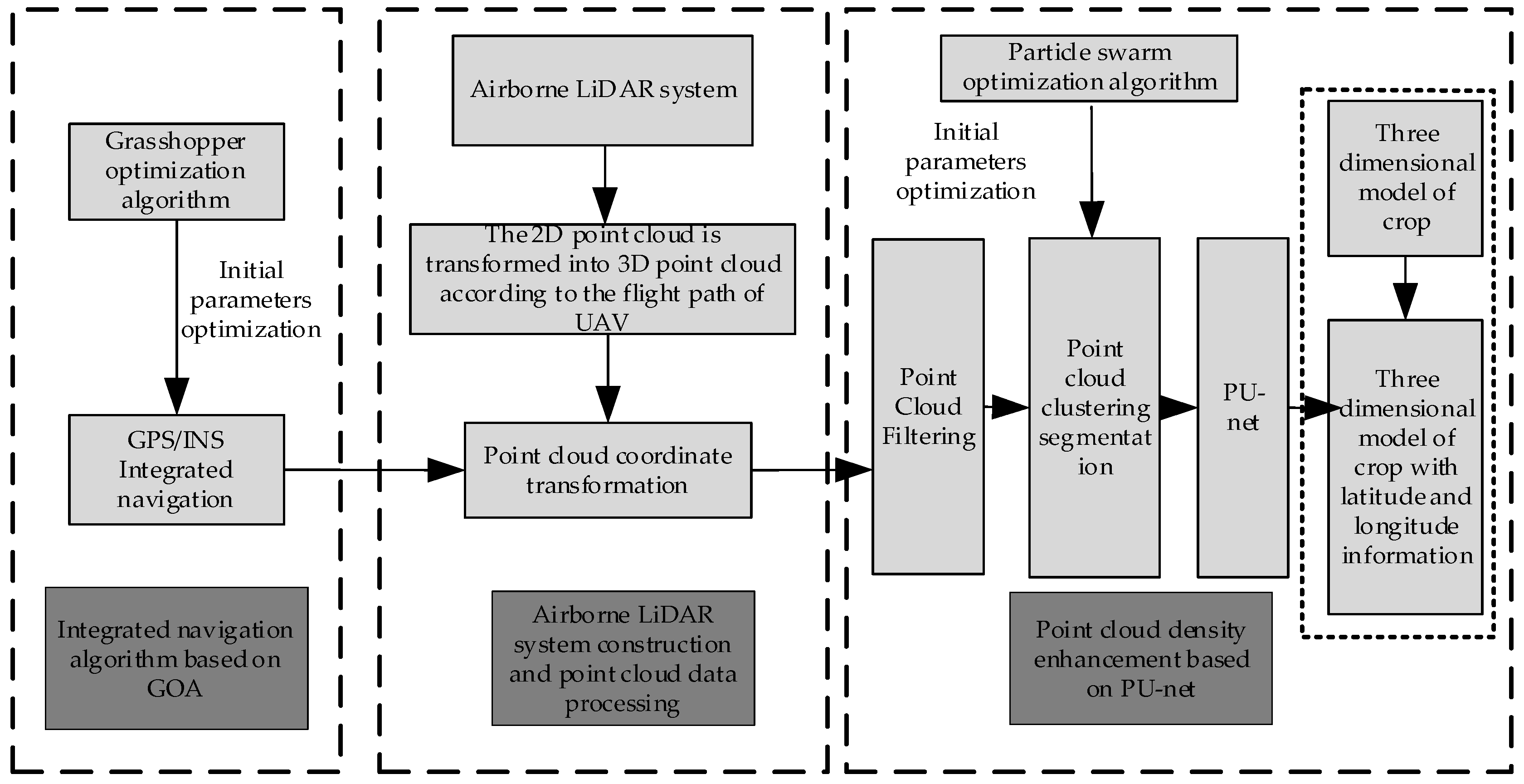
For UAV-borne LIDAR point cloud data enhancement, the integrated navigation algorithm based on GOA and the point cloud density enhancement algorithm based on neural network were shown in Figure 1. The specific implementation steps were as follows:

(1)

Firstly, the GPS/INS integrated navigation information fusion framework was built by the Kalman filter. Then, the GOA was used to optimize the initial parameters of the Kalman filter, and the optimal solution was returned to the Kalman filter to estimate the output state of the GPS/INS integrated navigation system;

(2)

After data acquisition, the point cloud data was transformed into the WGS-84 coordinate system from the LiDAR coordinate system. Then the point cloud data was filtered for removing the irrelevant points. Finally, the two-dimensional point cloud data was transformed into a three-dimensional point cloud according to the flight trajectory of UAV;

(3)

The PSO algorithm was employed to optimize the density clustering algorithm for crop point cloud segment. Then the crop point cloud data was fed into the trained network to obtain the crop point cloud data after the point cloud density was enhanced. Finally, the point cloud data was reconstructed in three dimensions.

3. Integrated Navigation Enhancement Based on GOA

In GPS/INS integrated navigation, the Kalman filter was usually used for fusing information of GPS and INS. The better the filter of integrated navigation was, the better it can integrate the advantages of each sensor. Since the GOA is not affected by the nonlinearity or scale, compared with other global optimization algorithms, it can find more effective optimal solutions with faster convergence speed [24].

3.1. Framework of GPS/INS Integrated Navigation

GPS and INS have complementary advantages. By combining GPS and INS in an appropriate way, their own drawbacks could be overcome, and the navigation accuracy would significantly improve. In order to improve the robustness of the system and reduce the complexity of the system, this paper adopted the loose combination mode to fuse the information of GPS and INS, as shown in Figure 2.

The state variables of the integrated navigation filter were composed of the random drift error, velocity error, and position error of INS gyroscope, as well as errors caused by the attitude angle and accelerometer. The equation of the state was as follows:

$$\widehat{\mathrm{X}}=\mathrm{F}\mathrm{X}+\mathrm{G}\mathrm{w}$$

(1)

The state variables of the INS integrated navigation system include longitude error, latitude error, velocity error in east and north directions, attitude angle error in east, north, and sky directions, random drift, and accelerometer bias error. The 13-dimensional equation of the state was as follows:

$${\widehat{\mathrm{X}}}_{\mathrm{I}}={\mathrm{F}}_{\mathrm{I}}{\mathrm{X}}_{\mathrm{I}}+{\mathrm{G}}_{\mathrm{I}}{\mathsf{\omega }}_{\mathrm{I}}$$

(2)

The clock error of the receiver equivalent distance $\mathsf{\delta }{\mathrm{t}}_{\mathrm{u}}$ and equivalent range error of the receiver clock frequency error $\mathsf{\delta }{\mathrm{t}}_{\mathrm{r}\mathrm{u}}$ were the GPS state errors; the equation of the state can be described as follows:

$${\widehat{\mathrm{X}}}_{\mathrm{G}}={\mathrm{F}}_{\mathrm{G}}{\mathrm{X}}_{\mathrm{G}}+{\mathrm{G}}_{\mathrm{G}}{\mathrm{w}}_{\mathrm{G}}$$

(3)

The measurement equation of the position velocity combination was expressed as follows:

$$\left[\begin{array}{c}{\mathrm{L}}_{\mathrm{I}\mathrm{N}\mathrm{S}}\\ {\mathsf{\lambda }}_{\mathrm{I}\mathrm{N}\mathrm{S}}\\ {\mathrm{h}}_{\mathrm{I}\mathrm{N}\mathrm{S}}\end{array}\right]=\left[\begin{array}{c}{\mathrm{L}}_{\mathrm{t}}+\mathsf{\delta }\mathrm{L}\\ {\mathsf{\lambda }}_{\mathrm{t}}+\mathsf{\delta }\mathsf{\lambda }\\ {\mathrm{h}}_{\mathrm{t}}+\mathsf{\delta }\mathrm{h}\end{array}\right]$$

(4)

where ${\mathrm{L}}_{\mathrm{I}\mathrm{N}\mathrm{S}}$, ${\mathsf{\lambda }}_{\mathrm{I}\mathrm{N}\mathrm{S}}$, and ${\mathrm{h}}_{\mathrm{I}\mathrm{N}\mathrm{S}}$ were the longitude, latitude, and altitude calculated by inertial navigation. ${\mathrm{L}}_{\mathrm{t}}$, ${\mathsf{\lambda }}_{\mathrm{t}}$, and ${\mathrm{h}}_{\mathrm{t}}$ were the real longitude, latitude, and height of the carrier. $\mathsf{\delta }\mathrm{L}$, $\mathsf{\delta }\mathsf{\lambda }$, and $\mathsf{\delta }\mathrm{h}$ were the longitude and latitude error and altitude error calculated by INS.

The position measurement information of the GPS receiver was expressed by subtracting the corresponding error from the real value:

$$\left[\begin{array}{c}{\mathrm{L}}_{\mathrm{G}\mathrm{P}\mathrm{S}}\\ {\mathsf{\lambda }}_{\mathrm{G}\mathrm{P}\mathrm{S}}\\ {\mathrm{h}}_{\mathrm{G}\mathrm{P}\mathrm{S}}\end{array}\right]=\left[\begin{array}{c}{\mathrm{L}}_{\mathrm{t}}-\frac{{\mathrm{N}}_{\mathrm{n}}}{\mathrm{R}}\\ {\mathsf{\lambda }}_{\mathrm{t}}-\frac{{\mathrm{N}}_{\mathrm{e}}}{\mathrm{R}\mathrm{c}\mathrm{o}\mathrm{s}\mathrm{L}}\\ {\mathrm{h}}_{\mathrm{t}}-{\mathrm{N}}_{\mathrm{u}}\end{array}\right]$$

(5)

where ${\mathrm{N}}_{\mathrm{n}}$, ${\mathrm{N}}_{\mathrm{e}}$, and ${\mathrm{N}}_{\mathrm{u}}$ were the position error of the GNSS receiver along the east, north, and sky directions. Then the external measurement position error can be defined as:

$${\mathrm{Z}}_{\mathrm{p}\mathrm{o}\mathrm{s}}=\left[\begin{array}{c}{\mathsf{\lambda }}_{\mathrm{I}\mathrm{N}\mathrm{S}}-{\mathsf{\lambda }}_{\mathrm{G}\mathrm{P}\mathrm{S}}\\ {\mathrm{L}}_{\mathrm{I}\mathrm{N}\mathrm{S}}-{\mathrm{L}}_{\mathrm{G}\mathrm{P}\mathrm{S}}\\ {\mathrm{h}}_{\mathrm{I}\mathrm{N}\mathrm{S}}-{\mathrm{h}}_{\mathrm{G}\mathrm{P}\mathrm{S}}\end{array}\right]$$

(6)

The position measurement equation was as follows:

$${\mathrm{Z}}_{\mathrm{P}\mathrm{O}\mathrm{S}}={\mathrm{H}}_{\mathrm{P}\mathrm{O}\mathrm{S}}\left(\mathrm{t}\right)\mathrm{X}\left(\mathrm{t}\right)+{\mathrm{V}}_{\mathrm{P}\mathrm{O}\mathrm{S}}\left(\mathrm{t}\right)$$

(7)

The velocity measurement information equation of INS can be expressed as follows:

$$\left[\begin{array}{c}{\mathrm{v}}_{\mathrm{e}\mathrm{I}\mathrm{N}\mathrm{S}}\\ {\mathrm{v}}_{\mathrm{n}\mathrm{I}\mathrm{N}\mathrm{S}}\\ {\mathrm{v}}_{\mathrm{u}\mathrm{I}\mathrm{N}\mathrm{S}}\end{array}\right]=\left[\begin{array}{c}{\mathrm{v}}_{\mathrm{e}}+\mathsf{\delta }{\mathrm{v}}_{\mathrm{e}}\\ {\mathrm{v}}_{\mathrm{n}}+\mathsf{\delta }{\mathrm{v}}_{\mathrm{n}}\\ {\mathrm{v}}_{\mathrm{u}}+\mathsf{\delta }{\mathrm{v}}_{\mathrm{u}}\end{array}\right]$$

(8)

where ${\mathrm{v}}_{\mathrm{e}\mathrm{I}\mathrm{N}\mathrm{S}}$, ${\mathrm{v}}_{\mathrm{n}\mathrm{I}\mathrm{N}\mathrm{S}}$, and ${\mathrm{v}}_{\mathrm{u}\mathrm{I}\mathrm{N}\mathrm{S}}$ were the east speed, north speed, and sky speed calculated by the inertial navigation system. ${\mathrm{v}}_{\mathrm{e}}$, ${\mathrm{v}}_{\mathrm{n}}$, and ${\mathrm{v}}_{\mathrm{u}}$ were the velocity of the object in the east, north, and sky directions.

The velocity information provided by GPS can be expressed by the difference between the real value and the corresponding error in the geographical coordinate system:

$$\left[\begin{array}{c}{\mathrm{v}}_{\mathrm{e}\mathrm{G}\mathrm{P}\mathrm{S}}\\ {\mathrm{v}}_{\mathrm{n}\mathrm{G}\mathrm{P}\mathrm{S}}\\ {\mathrm{v}}_{\mathrm{u}\mathrm{G}\mathrm{P}\mathrm{S}}\end{array}\right]=\left[\begin{array}{c}{\mathrm{v}}_{\mathrm{e}}-{\mathrm{M}}_{\mathrm{e}}\\ {\mathrm{v}}_{\mathrm{n}}-{\mathrm{M}}_{\mathrm{n}}\\ {\mathrm{v}}_{\mathrm{u}}-{\mathrm{M}}_{\mathrm{u}}\end{array}\right]$$

(9)

The speed error of the external measurement can be defined as:

$${\mathrm{Z}}_{\mathrm{v}\mathrm{e}\mathrm{l}}=\left[\begin{array}{c}{\mathrm{v}}_{\mathrm{e}\mathrm{I}\mathrm{N}\mathrm{S}}-{\mathrm{v}}_{\mathrm{e}\mathrm{G}\mathrm{P}\mathrm{S}}\\ {\mathrm{v}}_{\mathrm{n}\mathrm{I}\mathrm{N}\mathrm{S}}-{\mathrm{v}}_{\mathrm{n}\mathrm{G}\mathrm{P}\mathrm{S}}\\ {\mathrm{v}}_{\mathrm{u}\mathrm{I}\mathrm{N}\mathrm{S}}-{\mathrm{v}}_{\mathrm{u}\mathrm{G}\mathrm{P}\mathrm{S}}\end{array}\right]$$

(10)

The velocity measurement equation was as follows:

$${\mathrm{Z}}_{\mathrm{v}\mathrm{e}\mathrm{l}}={\mathrm{H}}_{\mathrm{v}\mathrm{e}\mathrm{l}}\left(\mathrm{t}\right)\mathrm{X}\left(\mathrm{t}\right)+{\mathrm{V}}_{\mathrm{v}\mathrm{e}\mathrm{l}}\left(\mathrm{t}\right)$$

(11)

The integrated measurement equation of the GPS/INS integrated navigation system was obtained as follows:

$$\mathrm{Z}(\mathrm{t})=\left[\begin{array}{c}{\mathsf{\lambda }}_{\mathrm{I}\mathrm{N}\mathrm{S}}-{\mathsf{\lambda }}_{\mathrm{G}\mathrm{P}\mathrm{S}}\\ {\mathrm{L}}_{\mathrm{I}\mathrm{N}\mathrm{S}}-{\mathrm{L}}_{\mathrm{I}\mathrm{N}\mathrm{S}}\\ {\mathrm{h}}_{\mathrm{I}\mathrm{N}\mathrm{S}}-{\mathrm{h}}_{\mathrm{I}\mathrm{N}\mathrm{S}}\\ {\mathrm{v}}_{\mathrm{e}\mathrm{I}\mathrm{N}\mathrm{S}}-{\mathrm{v}}_{\mathrm{e}\mathrm{G}\mathrm{P}\mathrm{S}}\\ {\mathrm{v}}_{\mathrm{n}\mathrm{I}\mathrm{N}\mathrm{S}}-{\mathrm{v}}_{\mathrm{n}\mathrm{G}\mathrm{P}\mathrm{S}}\\ {\mathrm{v}}_{\mathrm{u}\mathrm{I}\mathrm{N}\mathrm{S}}-{\mathrm{v}}_{\mathrm{u}\mathrm{I}\mathrm{N}\mathrm{S}}\end{array}\right]=\mathrm{H}(\mathrm{t})\mathrm{X}(\mathrm{t})+\mathrm{V}(\mathrm{t})$$

(12)

3.2. Grasshopper Optimization Algorithm (GOA)

GOA is a swarm intelligence optimization algorithm designed by Australian scholar Shahrzad [18] in 2017, simulating the predatory migration behaviors of the grasshopper population in nature. The main characteristics of larval stage grasshoppers were slow movement and small stride. In contrast, long distances and sudden movements were essential features of adult grasshoppers. Searching for food sources was another important feature of the grasshopper swarm. The mathematical model of grasshopper swarm behavior was as follows:

$${\mathrm{X}}_{\mathrm{i}}={\displaystyle \sum _{\begin{array}{l}\mathrm{j}=1\\ \mathrm{j}\ne \mathrm{i}\end{array}}^{\mathrm{N}}\mathrm{s}\left(|{\mathrm{x}}_{\mathrm{j}}-{\mathrm{x}}_{\mathrm{i}}|\right)\frac{{\mathrm{x}}_{\mathrm{j}}-{\mathrm{x}}_{\mathrm{i}}}{{\mathrm{d}}_{\mathrm{i}\mathrm{j}}}}-\mathrm{g}{\widehat{\mathrm{e}}}_{\mathrm{g}}+\mathrm{u}{\widehat{\mathrm{e}}}_{\mathrm{w}}$$

(13)

where ${\mathrm{X}}_{\mathrm{i}}$ represented the position of ${\mathrm{i}}_{\mathrm{t}\mathrm{h}}$ grasshopper. $\mathrm{N}$ represents the amount of the grasshopper swarm. $\mathrm{s}$ was interaction force between grasshoppers. ${\mathrm{d}}_{\mathrm{i}\mathrm{j}}$ was the distance between the ${\mathrm{i}}_{\mathrm{t}\mathrm{h}}$ grasshopper and ${\mathrm{j}}_{\mathrm{t}\mathrm{h}}$ grasshopper. The function of the interaction force (attraction and repulsion shown in Figure 3.) $s$ between grasshoppers was defined as follows:

$$\mathrm{s}\left(\mathrm{d}\right)=\mathrm{f}{\mathrm{e}}^{\frac{-\mathrm{d}}{\mathrm{l}}}-{\mathrm{e}}^{-\mathrm{d}}$$

(14)

where $\mathrm{d}$ was the distance between two grasshoppers. $\mathrm{f}$ represented the interaction force (attraction and repulsion), $\mathrm{l}$ represented the unit of interaction force length. The modified form of Equation (10) was as follows:

$${\mathrm{X}}_{\mathrm{i}}^{\mathrm{d}\mathrm{i}\mathrm{m}}=\mathrm{c}\ast \mathrm{r}\left({\displaystyle \sum _{\begin{array}{l}\mathrm{j}=1\\ \mathrm{j}\ne \mathrm{i}\end{array}}^{\mathrm{N}}\mathrm{c}\frac{\mathrm{u}{\mathrm{b}}_{\mathrm{d}\mathrm{i}\mathrm{m}}-\mathrm{l}{\mathrm{b}}_{\mathrm{d}\mathrm{i}\mathrm{m}}}{2}}\mathrm{A}\frac{{\mathrm{x}}_{\mathrm{j}}-{\mathrm{x}}_{\mathrm{i}}}{{\mathrm{d}}_{\mathrm{i}\mathrm{j}}}\right)+{\widehat{\mathrm{T}}}_{\mathrm{d}\mathrm{i}\mathrm{m}}$$

(15)

$$\mathrm{A}=\mathrm{s}\left(|{\mathrm{x}}_{\mathrm{j}}^{\mathrm{d}}-{\mathrm{x}}_{\mathrm{i}}^{\mathrm{d}}|\right)$$

(16)

where $\mathrm{u}{\mathrm{b}}_{\mathrm{d}\mathrm{i}\mathrm{m}}$ was the upper boundary of the $\mathrm{d}\mathrm{i}{\mathrm{m}}_{\mathrm{t}\mathrm{h}}$ dimension, $\mathrm{l}{\mathrm{b}}_{\mathrm{d}\mathrm{i}\mathrm{m}}$ was the lower boundary, and ${\widehat{\mathrm{T}}}_{\mathrm{d}\mathrm{i}\mathrm{m}}$ was the target value of the $\mathrm{d}\mathrm{i}{\mathrm{m}}_{\mathrm{t}\mathrm{h}}$ dimension. $\mathrm{c}$ represented a self-adaption ratio which is defined as follows:

$$\mathrm{c}={\mathrm{c}}_{\mathrm{m}\mathrm{a}\mathrm{x}}-\mathrm{l}\frac{{\mathrm{c}}_{\mathrm{m}\mathrm{a}\mathrm{x}}-{\mathrm{c}}_{\mathrm{m}\mathrm{i}\mathrm{n}}}{\mathrm{L}}$$

(17)

where ${\mathrm{c}}_{\mathrm{m}\mathrm{a}\mathrm{x}}$ was the max value, while ${\mathrm{c}}_{\mathrm{m}\mathrm{i}\mathrm{n}}$ was the minimum value; $\mathrm{l}$ represented the current iteration, while $\mathrm{L}$ is the max iteration.

3.3. Kalman Filter Optimization Using GOA

GOA was employed to optimize the initial parameters Q and R of the Kalman filter. Q was the variance matrix of the system noise sequence, which affected the filtering performance and parameter estimation accuracy of the Kalman filter algorithm; R was the variance matrix of the measurement noise sequence, which was related to the correction speed of filtering and the stability of the filtering process. Through the optimization of the initial parameters, the optimal position of the grasshopper was as close to the real value as possible, thus the accuracy of the Kalman filter algorithm was improved greatly. The sum of the variances of longitude and latitude errors was selected as the fitness function. The pipelines of the Kalman filter optimization was shown in Figure 4.

4. UAV-Borne LiDAR System Construction and Point Cloud Data Processing

The UAV-borne LiDAR system was mainly composed of the LiDAR sensor, GPS/INS integrated navigation module, and UAV carrier. After the point cloud data were collected by the UAV-borne LiDAR scanning system, it was necessary to transform the point cloud data from the LiDAR coordinate system to the WGS-84 coordinate system.

4.1. UAV-Borne LiDAR System

In view of the application of LiDAR in the agricultural field, this paper selected RPLiDAR-a2 of SLAMTEC^®, which was a single-line two-dimensional LiDAR, which greatly reduced the cost of equipment. The WitMotion^® GPS/ Inertial Measurement Unit (IMU) was selected to collect the navigation and positioning information of UAV. In order to supply electricity to the LiDAR and the IMU, a small pad was used to combine the system. DJI^® M100 UAV was selected as the carrier, which was a lightweight UAV. Finally, the UAV-borne LiDAR scanning system was completed, as shown in Figure 5 and Figure 6.

Due to the single scanning line of RPLiDAR-a2, the collected point cloud data was a two-dimensional point cloud, which only contained the data of Y and Z coordinates. In order to generate three-dimensional point cloud data, according to the light trajectory and speed of UAV, the data of the X-axis were inversely solved according to IMU.

4.2. Coordinate Transformation of Point Cloud Data

It was assumed that the coordinate of the laser foot point in the instantaneous laser coordinate system was $({\mathrm{x}}_{\mathrm{S}\mathrm{L}},{\mathrm{y}}_{\mathrm{S}\mathrm{L}},{\mathrm{z}}_{\mathrm{S}\mathrm{L}}{)}^{\mathrm{T}}$:

$$\left[\begin{array}{l}{\mathrm{x}}_{\mathrm{S}\mathrm{L}}\\ {\mathrm{y}}_{\mathrm{S}\mathrm{L}}\\ {\mathrm{z}}_{\mathrm{S}\mathrm{L}}\end{array}\right]=\left[\begin{array}{l}0\\ 0\\ \mathsf{\rho }\end{array}\right]$$

(18)

There was an angle $\theta$ between the instantaneous laser coordinate system and the laser scanning reference coordinate system. The coordinates of the raw point cloud data in the laser scanning reference coordinate system were ${({\mathrm{x}}_{\mathrm{L}},{\mathrm{y}}_{\mathrm{L}},{\mathrm{z}}_{\mathrm{L}})}^{\mathrm{T}}$:

$$\left[\begin{array}{l}{\mathrm{x}}_{\mathrm{L}}\\ {\mathrm{y}}_{\mathrm{L}}\\ {\mathrm{z}}_{\mathrm{L}}\end{array}\right]={\mathrm{R}}_{\mathrm{L}}\left[\begin{array}{l}{\mathrm{x}}_{\mathrm{S}\mathrm{L}}\\ {\mathrm{y}}_{\mathrm{S}\mathrm{L}}\\ {\mathrm{z}}_{\mathrm{S}\mathrm{L}}\end{array}\right]$$

(19)

where ${\mathrm{R}}_{\mathrm{L}}$ represented the rotation matrix of scan angle $\theta$.

Generally, the error between the different coordinate axes was analyzed and unified to be the placement error angle $\mathsf{\alpha }$, $\mathsf{\beta }$, and $\mathsf{\gamma }$. The deviation of the coordinate origin and reference center was treated as error ${\mathrm{t}}_{\mathrm{L}}={(\Delta {\mathrm{x}}_{\mathrm{I}}^{\mathrm{L}},\Delta {\mathrm{y}}_{\mathrm{I}}^{\mathrm{L}},\Delta {\mathrm{z}}_{\mathrm{I}}^{\mathrm{L}})}^{\mathrm{T}}$. The coordinates of the raw point cloud in the inertial platform reference coordinate system were ${({\mathrm{x}}_{\mathrm{I}},{\mathrm{y}}_{\mathrm{I}},{\mathrm{z}}_{\mathrm{I}})}^{\mathrm{T}}$:

$$\left[\begin{array}{l}{\mathrm{x}}_{\mathrm{I}}\\ {\mathrm{y}}_{\mathrm{I}}\\ {\mathrm{z}}_{\mathrm{I}}\end{array}\right]={\mathrm{R}}_{\mathrm{M}}\left[\begin{array}{l}{\mathrm{x}}_{\mathrm{L}}\\ {\mathrm{y}}_{\mathrm{L}}\\ {\mathrm{z}}_{\mathrm{L}}\end{array}\right]+\left[\begin{array}{l}\Delta {\mathrm{x}}_{\mathrm{I}}^{\mathrm{L}}\\ \Delta {\mathrm{y}}_{\mathrm{I}}^{\mathrm{L}}\\ \Delta {\mathrm{z}}_{\mathrm{I}}^{\mathrm{L}}\end{array}\right]$$

(20)

where ${\mathrm{R}}_{\mathrm{M}}=\mathrm{R}(\mathsf{\gamma })\times \mathrm{R}(\mathsf{\beta })\times \mathrm{R}(\mathsf{\alpha })$.

In the integrated navigation system, there were also positioning errors between GPS and INS. During the installation process, there was a certain deviation between the center of GPS and the reference center of inertial components. The deviation was defined as ${\mathrm{t}}_{\mathrm{G}}={(\Delta {\mathrm{x}}_{\mathrm{I}}^{\mathrm{G}},\Delta {\mathrm{y}}_{\mathrm{I}}^{\mathrm{G}},\Delta {\mathrm{z}}_{\mathrm{I}}^{\mathrm{G}})}^{\mathrm{T}}$; it can be measured offline. INS measured the attitude information of the carrier in real time, including roll angle (R), pitch angle (P), and heading angle (H), and got the velocity and position information of the carrier through integration and feed back to the user in real time. At the same time, the coordinate rotation matrix was obtained by calculating the attitude information feedback from IMU. The coordinates of the raw point cloud data in the local reference coordinate system were ${({\mathrm{x}}_{\mathrm{L}\mathrm{H}},{\mathrm{y}}_{\mathrm{L}\mathrm{H}},{\mathrm{z}}_{\mathrm{L}\mathrm{H}})}^{\mathrm{T}}$:

$$\left[\begin{array}{c}{\mathrm{x}}_{\mathrm{L}\mathrm{H}}\\ {\mathrm{y}}_{\mathrm{L}\mathrm{H}}\\ {\mathrm{z}}_{\mathrm{L}\mathrm{H}}\end{array}\right]={\mathrm{R}}_{\mathrm{N}}\left[\begin{array}{c}{\mathrm{x}}_{\mathrm{I}}\\ {\mathrm{y}}_{\mathrm{I}}\\ {\mathrm{z}}_{\mathrm{I}}\end{array}\right]-\left[\begin{array}{c}\Delta {\mathrm{x}}_{\mathrm{I}}^{\mathrm{G}}\\ \Delta {\mathrm{y}}_{\mathrm{I}}^{\mathrm{G}}\\ \Delta {\mathrm{z}}_{\mathrm{I}}^{\mathrm{G}}\end{array}\right]$$

(21)

where ${\mathrm{R}}_{\mathrm{N}}=\mathrm{R}(\mathrm{H})\times \mathrm{R}(\mathrm{P})\times \mathrm{R}(\mathrm{R})$.

Finally, point cloud data should be transformed to WGS-84 coordinate system. The rotation matrix ${\mathrm{R}}_{\mathrm{w}}$ was a function of the latitude and longitude of the region. The point cloud could be transformed into the WGS-84 coordinate system by rotating the matrix:

$$\left[\begin{array}{l}{\mathrm{x}}_{84}\\ {\mathrm{y}}_{84}\\ {\mathrm{z}}_{84}\end{array}\right]={\mathrm{R}}_{\mathrm{W}}\left[\begin{array}{l}{\mathrm{x}}_{\mathrm{L}\mathrm{H}}\\ {\mathrm{y}}_{\mathrm{L}\mathrm{H}}\\ {\mathrm{z}}_{\mathrm{L}\mathrm{H}}\end{array}\right]+{\left[\begin{array}{l}{\mathrm{x}}_{84}\\ {\mathrm{y}}_{84}\\ {\mathrm{z}}_{84}\end{array}\right]}_{\mathrm{A}\mathrm{n}\mathrm{t}\mathrm{e}\mathrm{n}\mathrm{n}\mathrm{a} \mathrm{p}\mathrm{h}\mathrm{a}\mathrm{s}\mathrm{e} \mathrm{c}\mathrm{e}\mathrm{n}\mathrm{t}\mathrm{e}\mathrm{r}}$$

(22)

Based on the above analysis, the coordinates of the raw point cloud in WGS-84 coordinate system were as follows:

$$\left[\begin{array}{l}{\mathrm{x}}_{84}\\ {\mathrm{y}}_{84}\\ {\mathrm{z}}_{84}\end{array}\right]={\mathrm{R}}_{\mathrm{W}}{\mathrm{R}}_{\mathrm{N}}\left[{\mathrm{R}}_{\mathrm{M}}{\mathrm{R}}_{\mathrm{L}}\left[\begin{array}{l}0\\ 0\\ \mathsf{\rho }\end{array}\right]+\left[\begin{array}{l}\Delta {\mathrm{x}}_{\mathrm{I}}^{\mathrm{L}}\\ \Delta {\mathrm{y}}_{\mathrm{I}}^{\mathrm{L}}\\ \Delta {\mathrm{z}}_{\mathrm{I}}^{\mathrm{L}}\end{array}\right]-\left[\begin{array}{l}\Delta {\mathrm{x}}_{\mathrm{I}}^{\mathrm{G}}\\ \Delta {\mathrm{y}}_{\mathrm{I}}^{\mathrm{G}}\\ \Delta {\mathrm{z}}_{\mathrm{I}}^{\mathrm{G}}\end{array}\right]\right]+{\left[\begin{array}{l}{\mathrm{x}}_{84}\\ {\mathrm{y}}_{84}\\ {\mathrm{z}}_{84}\end{array}\right]}_{\mathrm{A}\mathrm{n}\mathrm{t}\mathrm{e}\mathrm{n}\mathrm{n}\mathrm{a} \mathrm{p}\mathrm{h}\mathrm{a}\mathrm{s}\mathrm{e} \mathrm{c}\mathrm{e}\mathrm{n}\mathrm{t}\mathrm{e}\mathrm{r}}$$

(23)

In addition, in order to get the data containing the latitude and longitude information, it was necessary to convert the three-dimensional rectangular coordinates ($\mathrm{X}\mathrm{Y}\mathrm{Z}$) into geodetic coordinates ($\mathsf{\lambda }\mathrm{L}\mathrm{H}$). The conversion formula was as follows:

$$\mathrm{L}=\mathrm{a}\mathrm{r}\mathrm{c}\mathrm{t}\mathrm{a}\mathrm{n}\left(\mathrm{Y}/\mathrm{X}\right)$$

(24)

$$\mathsf{\lambda }=\mathrm{a}\mathrm{r}\mathrm{c}\mathrm{t}\mathrm{a}\mathrm{n}\left[\mathrm{Z}/\sqrt{{\mathrm{X}}^2+{\mathrm{Y}}^2}\ast {\left(1-{\mathrm{e}}^2\mathrm{N}\left(\mathrm{N}+\mathrm{H}\right)\right)}^{-1}\right]$$

(25)

$$\mathrm{H}=\sqrt{{\mathrm{X}}^2+{\mathrm{Y}}^2}/\mathrm{c}\mathrm{o}\mathrm{s}\mathsf{\lambda }-\mathrm{N}$$

(26)

where $\mathrm{X}$, $\mathrm{Y}$, and $\mathrm{Z}$ were three-dimensional rectangular coordinate components, $\mathrm{L}$, $\mathsf{\lambda }$, and $H$ were earth longitude, latitude, and height. $\mathrm{e}$ represented the first eccentricity of the ellipsoid. $\mathrm{N}=\mathrm{a}/\sqrt{1-{\mathrm{e}}^2\mathrm{s}\mathrm{i}{\mathrm{n}}^2\mathsf{\lambda }}$ was the radius of curvature in the prime vertical, and the $\mathrm{a}$ was the semimajor axis of the ellipsoid.

5. Point Cloud Density Enhancement Based on PU-Net

Point cloud density enhancement aims to increase the number of point clouds without destroying the characteristics of the original point cloud. By enhancing the density of point cloud, the richness and accuracy of 3D reconstruction of point cloud data can be improved without increasing equipment cost.

5.1. Point Cloud Preprocessing

After the coordinate transformation, it was necessary to remove irrelevant noise points from the original point cloud data. In this paper, the statistical filtering method was selected for filtering. Statistical filtering calculated the distance between each point and its surrounding neighborhood points: According to neighborhood points and the standard deviation threshold, the points which did not meet the requirements were identified as outlier points.

5.2. Point Cloud Density Clustering Segmentation Method Based on PSO Algorithm

After filtering in the previous section, the point cloud data obtained included ground and crop points. In order to separate the ground and crop, the density clustering algorithm was used for separating, and the linear decreasing PSO algorithm was employed to improve the density clustering algorithm.

DBSCAN was a density-based clustering algorithm proposed by ester et al. It was designed to achieve clustering and segmentation of arbitrary data in spatial and non-spatial high-dimensional databases. By calculating the distance between each point and its neighborhood, the points with similar density were classified into the same class.

$\epsilon$-Neighborhood of arbitrary point $\mathrm{p}$ is defined as follows:

$${\mathrm{N}}_{\mathrm{e}\mathrm{p}\mathrm{s}}=\left\{\mathrm{q}\in \mathrm{D}/\mathrm{d}\mathrm{i}\mathrm{s}\mathrm{t}\left(\mathrm{p},\mathrm{q}\right)<\mathrm{E}\mathrm{p}\mathrm{s}\right\}$$

(27)

where $\mathrm{D}$ represented the target’s database, point $\mathrm{p}$ was the core point if the $\mathsf{\epsilon }$-neighborhood contained at least the minimum number of points. The core point was defined as follows:

$${\mathrm{N}}_{\mathrm{e}\mathrm{p}\mathrm{s}}\left(\mathrm{P}\right)>\mathrm{M}\mathrm{i}\mathrm{n}\mathrm{P}\mathrm{t}\mathrm{s}$$

(28)

where $\mathrm{E}\mathrm{p}\mathrm{s}$ and $\mathrm{M}\mathrm{i}\mathrm{n}\mathrm{P}\mathrm{t}\mathrm{s}$ were the neighborhood radius and minimum number of points in the $\epsilon$-neighborhood of the core point. Through the calculation of all the points, the density of the points meeting the set conditions was similar, and they were classified as the same kind of points. All points were calculated until the termination condition was met. Because the selection of these two initial parameters mainly depended on human experience and continuous experiments, in order to improve the efficiency, this paper employed the linear decreasing PSO algorithm to iteratively optimize the two initial parameters to determine the optimal solution of the initial parameters.

The PSO algorithm was a swarm intelligent bionic optimization algorithm: Every point in PSO was stamped by a position ${\mathrm{P}}_{\mathrm{i}}$, the optimal value of swarm was ${\mathrm{P}}_{\mathrm{g}}$, every point’s velocity was ${\mathrm{V}}_{\mathrm{i}}$, and each particle’s velocity and position update formula was shown as follows:

$${\mathrm{V}}_{\mathrm{i}}^{\mathrm{t}+1}=\mathsf{\omega }{\mathrm{V}}_{\mathrm{i}}^{\mathrm{t}}+{\mathrm{c}}_1{\mathrm{r}}_1({\mathrm{P}}_{\mathrm{i}}-{\mathrm{X}}_{\mathrm{i}}^{\mathrm{t}})+{\mathrm{c}}_2{\mathrm{r}}_2({\mathrm{P}}_{\mathrm{g}}-{\mathrm{X}}_{\mathrm{i}}^{\mathrm{t}})$$

(29)

$${\mathrm{X}}_{\mathrm{i}}^{\mathrm{t}+1}={\mathrm{X}}_{\mathrm{i}}^{\mathrm{t}}+{\mathrm{V}}_{\mathrm{i}}^{\mathrm{t}+1}$$

(30)

where $\mathrm{t}$ represented the iterations, ${\mathrm{V}}_{\mathrm{i}}^{\mathrm{t}+1}$ was the velocity of the $\mathrm{t}+1$ iteration, $\mathsf{\omega }$ represented the inertia weight. ${\mathrm{c}}_1$, ${\mathrm{c}}_2\in \left[0,1\right]$ were the generating functions of a random number, and ${\mathrm{X}}_{\mathrm{i}}^{\mathrm{t}+1}$ was the $\mathrm{t}+1$ iteration position.

In the initial stage of the algorithm, the inertia weight $\mathsf{\omega }$ was given a larger value to enhance the global exploration ability of the algorithm. With the continuous exploration process, the value of $\mathsf{\omega }$ could be linearly reduced to enhance the local search and optimization ability of the algorithm, so that particles could gradually approach the optimal solution in the neighborhood of the optimal value. The value of $\mathsf{\omega }$ was expressed as follows:

$$\mathsf{\omega }={\mathsf{\omega }}_{\mathrm{m}\mathrm{i}\mathrm{n}}+\frac{({\mathsf{\omega }}_{\mathrm{m}\mathrm{a}\mathrm{x}}-{\mathsf{\omega }}_{\mathrm{m}\mathrm{i}\mathrm{n}})\times (\mathrm{m}\mathrm{a}{\mathrm{x}}_{\mathrm{i}\mathrm{t}\mathrm{e}\mathrm{r}}-\mathrm{t})}{\mathrm{m}\mathrm{a}{\mathrm{x}}_{\mathrm{i}\mathrm{t}\mathrm{e}\mathrm{r}}}$$

(31)

where ${\mathsf{\omega }}_{\mathrm{m}\mathrm{a}\mathrm{x}}$ represented the max inertia coefficient, while ${\mathsf{\omega }}_{\mathrm{m}\mathrm{i}\mathrm{n}}$ represented the minimum. $\mathrm{m}\mathrm{a}{\mathrm{x}}_{\mathrm{i}\mathrm{t}\mathrm{e}\mathrm{r}}$ was the max iteration.

PSO optimization pipelines are shown in Figure 7:

5.3. Point Cloud Density

The point cloud data acquired by UAV-borne LiDAR was 3-dimensional, which was usually expressed by plane density. The point cloud density in national standards was defined as the normal direction of elevation density [22]:

$$\mathsf{\rho }=\frac{\mathrm{N}-{\displaystyle \sum _{\mathrm{i}=0}^{\mathrm{k}}{\mathrm{N}}_{\mathrm{i}}}}{\mathrm{A}-{\displaystyle \sum _{\mathrm{i}=0}^{\mathrm{k}}{\mathrm{A}}_{\mathrm{i}}}}$$

(32)

where $\mathsf{\rho }$ represented the point cloud density, and $\mathrm{N}$ represented the total amount of points. Furthermore, ${\mathrm{N}}_{\mathrm{i}}$ was the ${\mathrm{i}}_{\mathrm{t}\mathrm{h}}$ field number of points, and $\mathrm{k}$ was the number of scanning area. $\mathrm{A}$ was the measure of the scanning area.

The point cloud density calculated by the above formula was the average point cloud density in the scanning area. In order to further quantify the point density distribution in the scanning area, the reciprocal of the area affected by a single point was taken as the density of the point:

$${\mathrm{d}}^{\prime }=1/{\mathrm{A}}^{\prime }$$

(33)

The main factors affecting the density of the point cloud were the LiDAR design parameters, system characteristics, carrier, and scanning area.

The distance between points directly reflected the density of point clouds. For the pulse laser ranging sensor, the distance from the heading point to the edge point determined the density distribution of point cloud. The design of aerial photography parameters was referred from the distance between heading point and edge point. The parameters of the sensor, such as scanning frequency, scanning bandwidth, laser emission frequency, field of view angle, flight height and flight speed, and the distance between point clouds, were considered to design the LiDAR system.

5.4. Density Enhancement Using Point Cloud Up-Sampling Network (PU-Net)

Point cloud up-sampling was essentially similar to the problem of image super-resolution [25]. Yu et al. [26] proposed a data-driven point cloud sampling neural network (PU-net), which was applied to patch level. At the same time, a joint loss function was used for guiding the up-sampled points to retain a uniformly distributed object surface. The main idea of PU-net was capturing the features of each point in every level, then multi-convolution blocks were extended in feature hidden layers, and finally, the hidden layers were divided into multi-level features and up-sampled into the point cloud. The pre-trained PU-net was employed for enhancing the density of the crop point cloud in this paper. There were 4 steps of PU-net for up-sampling of point cloud: Slice extraction, point feature embedding, feature extending, and point coordinate reconstruction. It is noteworthy that a series of sub-pixel convolution layers were employed to extend the features of neighborhood points in the feature extending stage:

$${\mathrm{f}}^{\prime }=\mathrm{R}\mathrm{e}\mathrm{s}\mathrm{h}\mathrm{a}\mathrm{p}\mathrm{e}([\mathrm{c}\mathrm{o}\mathrm{n}{\mathrm{v}}_1^2(\mathrm{c}\mathrm{o}\mathrm{n}{\mathrm{v}}_1^1(\mathrm{f})),\dots ,\mathrm{c}\mathrm{o}\mathrm{n}{\mathrm{v}}_{\mathrm{r}}^2(\mathrm{c}\mathrm{o}\mathrm{n}{\mathrm{v}}_{\mathrm{r}}^1(\mathrm{f}))])$$

(34)

where $\mathrm{c}\mathrm{o}\mathrm{n}{\mathrm{v}}_{\mathrm{i}}^1({}^{*})$ and $\mathrm{c}\mathrm{o}\mathrm{n}{\mathrm{v}}_{\mathrm{i}}^2({}^{*})$ were the convolution layer with 1*1 kernel size for adjusting the channels of patch feature $\mathrm{f}$. The output, combined feature ${\mathrm{f}}^{\prime }$, was born with properties of spatial characteristic which could retain the information of raw data. After coordinate reconstruction, the density elevation in last section was employed to show the enhancement effect directly.

6. Results

In order to verify the stability of the UAV-borne LiDAR scanning system, the experiments were carried out in integrated navigation testing, point cloud density clustering, and point cloud density enhancement.

6.1. GOA-Based Integrated Navigation

The integrated navigation experiment was carried out in MATLAB2017 (a). It was supposed that the initial longitude of UAV $\mathrm{L}=40^{\mathrm{o}}$, the initial latitude $\mathsf{\lambda }=116^{\mathrm{o}}$, and the velocity of UAV was $1\mathrm{m}/\mathrm{s}$. The filtering period was $\mathrm{T}=1\mathrm{s}$. The initial value of filtering covariance was as follows:

$$\begin{array}{l}\mathrm{p}(0)=\mathrm{d}\mathrm{i}\mathrm{a}\mathrm{g}[{(0.00254^{\mathrm{o}})}^2,{(0.00446^{\mathrm{o}})}^2,{(0.1\mathrm{m}/\mathrm{s})}^2,\\ {(0.1\mathrm{m}/\mathrm{s})}^2,{(1^{\mathrm{o}})}^2,{(1^{\mathrm{o}})}^2,{(1^{\mathrm{o}})}^2,{(1^{\mathrm{o}})}^2,\\ {(1^{\mathrm{o}})}^2,{(1^{\mathrm{o}})}^2,({10}^{-5})\mathrm{g},(10^{-5})\mathrm{g},(10^{-5})\mathrm{g}]\end{array}$$

(35)

The initial value of integrated navigation was:

$$\begin{array}{l}\mathrm{X}(0)=[0\mathrm{m},0\mathrm{m},0.5\mathrm{m}/\mathrm{s},0.5\mathrm{m}/\mathrm{s},0.08^{\mathrm{o}},0.08^{\mathrm{o}},\\ 0.08^{\mathrm{o}},0.16^{\mathrm{o}},{0.1}^{\mathrm{o}}/\mathrm{h},{0.1}^{\mathrm{o}}/\mathrm{h},{0.1}^{\mathrm{o}}/\mathrm{h},\\ {0.1}^{\mathrm{o}}/\mathrm{h},(10^{-5})\mathrm{g},(10^{-5})\mathrm{g},(10^{-5})\mathrm{g}]\end{array}$$

(36)

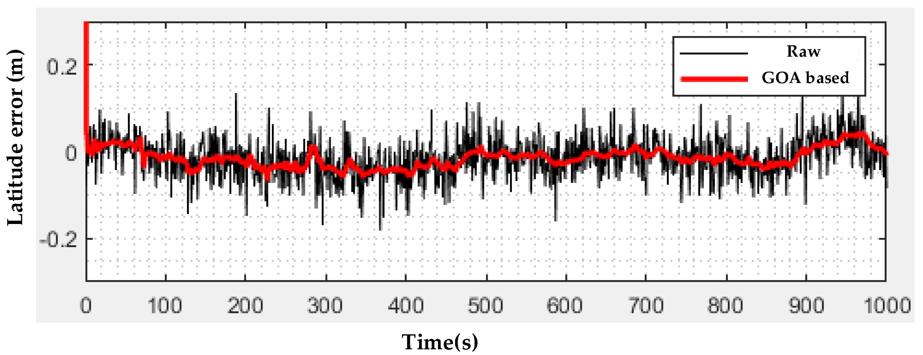
The initial parameters Q and R obtained when the sum of longitude and latitude errors were used as the fitness function feeding into the system. The GOA based integrated navigation error diagram was shown in Figure 8 and Figure 9, PSO based integrated navigation error diagram was shown in Figure 10 and Figure 11.

As shown in

Table 1. Error of integrated navigation with different enhancement methods.

	Longitude $\mathit{L}$ Variance Error	Latitude $\mathit{\lambda }$ Variance Error
GOA-based integrated navigation	0.00046	0.00034
PSO-based integrated navigation	0.00087	0.00079
Raw integrated navigation	0.0091	0.0047

, both the longitude $L$ variance error and latitude $\mathsf{\lambda }$ variance error were reduced greatly compared with raw integrated navigation. It is worth noting that the GOA-based integrated navigation showed better performance than the PSO-based integrated navigation; it is suspected that the ability to find the optimal of GOA was better than for PSO in the integrated navigation task. For more precise optimal Q and R, the GOA-based integrated navigation was employed for the UAV-borne LiDAR scanning system.

6.2. PSO-Based Point Cloud Clustering Segmentation

The meta-heuristic algorithm was employed to optimizing the clustering segmentation key elements: $\mathrm{E}\mathrm{p}\mathrm{s}$ and $\mathrm{M}\mathrm{i}\mathrm{n}\mathrm{P}\mathrm{t}\mathrm{s}$. The Davies–Bouldin index (DBI) was employed as the fitness function for the joint optimization of $\mathrm{E}\mathrm{p}\mathrm{s}$ and $\mathrm{M}\mathrm{i}\mathrm{n}\mathrm{P}\mathrm{t}\mathrm{s}$:

$$\mathrm{D}\mathrm{B}\mathrm{I}=\frac{1}{\mathrm{k}}{\displaystyle \sum _{\mathrm{i}=1}^{\mathrm{k}}\underset{\mathrm{j}\ne \mathrm{i}}{\mathrm{m}\mathrm{a}\mathrm{x}}\left(\frac{\mathrm{a}\mathrm{v}\mathrm{g}\left({\mathrm{C}}_{\mathrm{i}}\right)+\mathrm{a}\mathrm{v}\mathrm{g}\left({\mathrm{C}}_{\mathrm{j}}\right)}{{\mathrm{d}}_{\mathrm{c}\mathrm{e}\mathrm{n}}\left({\mathsf{\mu }}_{\mathrm{i}},{\mathsf{\mu }}_{\mathrm{j}}\right)}\right)}$$

(37)

where $\mathrm{a}\mathrm{v}\mathrm{g}(\ast )$ represented the average distance between samples in cluster, ${\mathrm{d}}_{\mathrm{c}\mathrm{e}\mathrm{n}}\left({\mathsf{\mu }}_{\mathrm{i}},{\mathsf{\mu }}_{\mathrm{j}}\right)$ was the center distance of cluster ${\mathsf{\mu }}_{\mathrm{i}}$, and cluster ${\mathsf{\mu }}_{\mathrm{j}}$. $\mathrm{a}\mathrm{v}\mathrm{g}({}^{*})$ was defined as follows:

$$\mathrm{a}\mathrm{v}\mathrm{g}\left(\mathrm{C}\right)=\frac{2}{\left|\mathrm{C}\right|\left(\left|\mathrm{C}\right|-1\right)}{\displaystyle {\sum }_{1\le \mathrm{i}\le \mathrm{j}\le \left|\mathrm{C}\right|}\mathrm{d}\mathrm{i}\mathrm{s}\mathrm{t}\left({\mathrm{x}}_{\mathrm{i}},{\mathrm{x}}_{\mathrm{j}}\right)}$$

(38)

where $\mathrm{d}\mathrm{i}\mathrm{s}\mathrm{t}\left({\mathrm{x}}_{\mathrm{i}},{\mathrm{x}}_{\mathrm{j}}\right)$ was the distance of sample ${\mathrm{x}}_{\mathrm{i}}$ and sample ${\mathrm{x}}_{\mathrm{j}}$.

Crop point cloud data collection environment was shown in Figure 12.

A series of crop point cloud raw data was collected from the UAV-borne LiDAR scanning system; the meta-heuristic-based DBSCAN algorithms were initialized by crop raw data and iterated 200 times to find the optimal Eps and MinPts. The fitness iteration curve is shown in Figure 13.

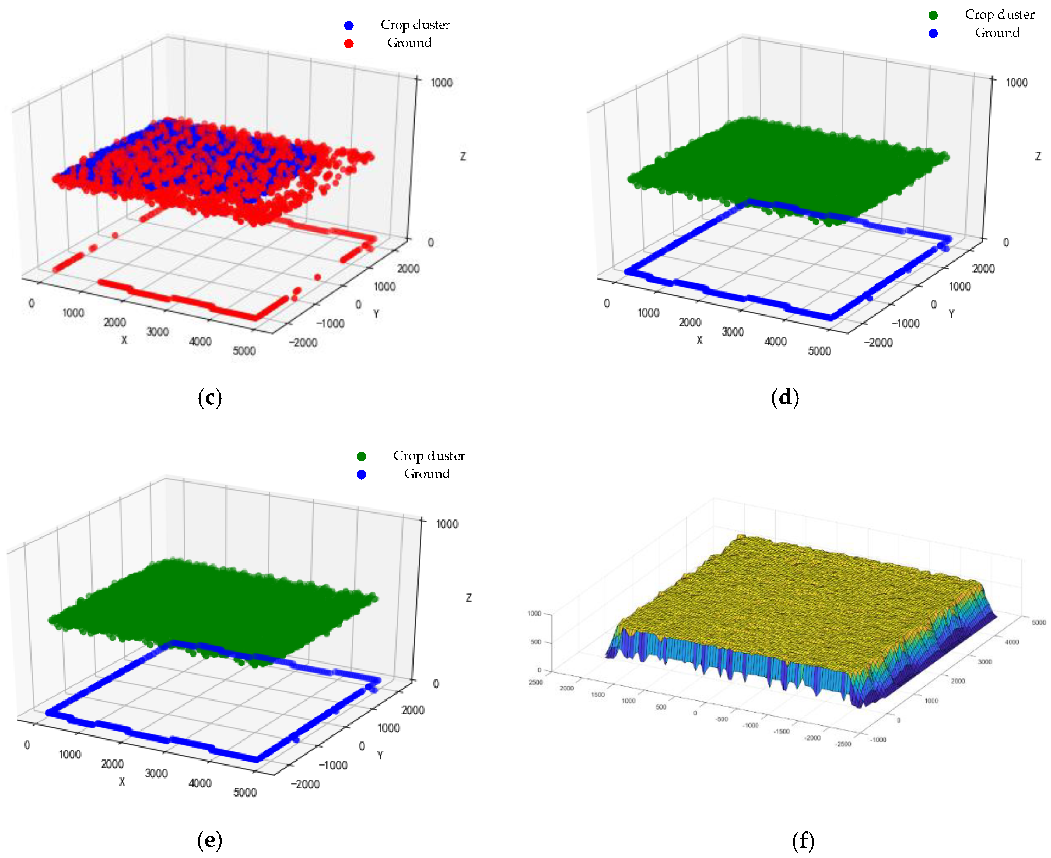
For fair comparing with different meta-heuristic algorithms, the BA-based DBSCAN algorithm [17], GA-based DBSCAN algorithm [14], GOA-based DBSCAN algorithm [18], and PSO-based DBSCAN algorithm [15] were initialized with 20 population-sizes, 2 dimensions, and 200 iterations. In particular, the GA-based DBSCAN algorithm was initialized with a 0.7 crossover rate, 0.5 select rate, and 0.01 variation rate. During several times of testing, Figure 13 shows that the GOA and PSO found the best fitness 0.416032. It is suspected that global optimization was 0.416032 under further testing with different fine tuning. Under the same fitness 0.416032, the Eps = 0.8147 and MinPts = 13. In the clustering segmentation, the BA-based DBSCAN algorithm, GA-based DBSCAN algorithm, GOA-based DBSCAN algorithm, PSO-based DBSCAN algorithm, and the K-means clustering were employed for comparison; the K-means was the default tuning. The 200 iterations of time consumption of the BA-based DBSCAN algorithm, GA-based DBSCAN algorithm, GOA-based DBSCAN algorithm, and PSO-based DBSCAN algorithm were 9669 s, 910 s, 1610 s, and 749 s, respectively. The comparison clustering results are shown in Figure 14a–e. Shown in Figure 14f, the crop point cloud is reconstructed in 3-dimensions.

As shown in Figure 14a–c, 3 kinds of clustering results were given from the default tuning of K-means, and the ground cluster could not be separated from the crop cluster using the BA-based DBSCAN algorithm or GA-based DBSCAN algorithm. Under the same fitness 0.416032, the Eps = 0.8147 and MinPts = 13 were obtained using the GOA-based DBSCAN algorithm and PSO-based DBSCAN algorithm. Considering that PSO converges faster and takes less time in iterations, the PSO-based DBSCAN algorithm was employed for crop point cloud clustering segmentation.

6.3. Density Enhancement with PU-Net

After the clustering segmentation of crop point cloud, the crop point cloud was enhanced by a pre-trained PU-net. The PU-net was trained with 60 sets of variation of point clouds from “Visionair”. Datasets were divided into train sets and validation sets by 60% and 40%. In the fine-tune training period, the Monte Carlo stochastic sampling method was employed for sampling 5000 points from every object as the input. Each input represented the global information of each object; fine-tune training aimed at enhancing the global information collection performance of the pretrained model. The visualization of raw crop point cloud data was shown in Figure 15. The sparse part of the point cloud was mainly concentrated on the X-axis, which was the direction of the UAV-borne LiDAR scanning system to generate the 3D point cloud by moving forward.

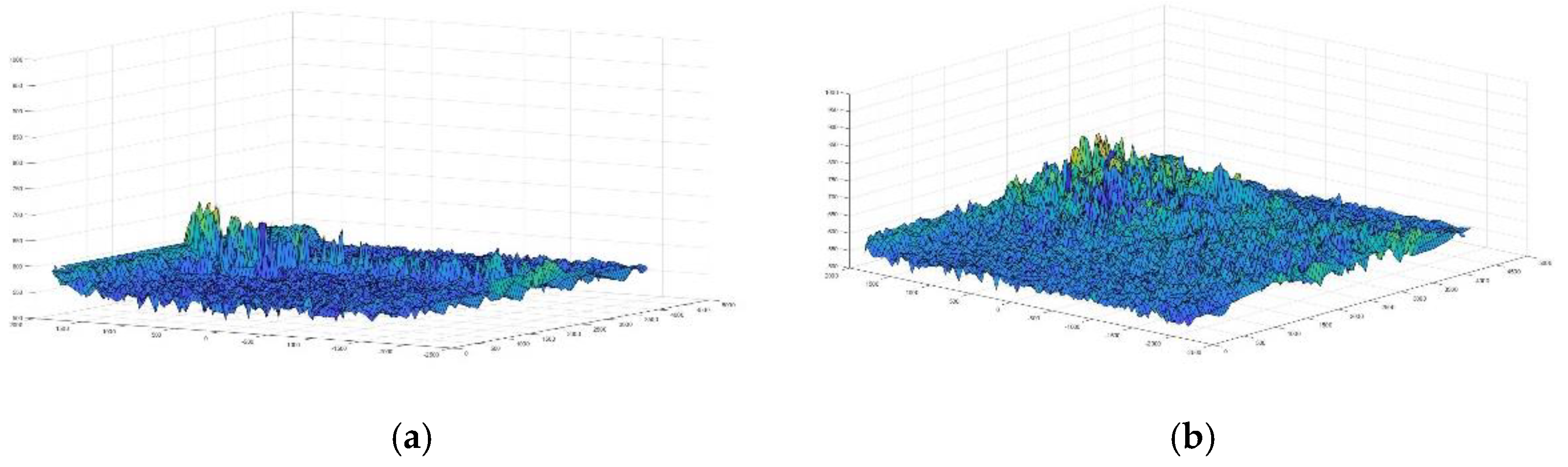
The raw crop point cloud was fed into the fine-tune trained PU-net. The 3D reconstruction of the crop point cloud with and without density enhancement is shown in Figure 16.

The total number of points of the raw crop point cloud were 10,000, the density of the raw crop point cloud was 1250 points per square meter. After density enhancement, the total number of points of the crop point cloud were 40,000, the density of the crop point cloud was 5000 points per square meter, and the number and density of the point cloud had been significantly increased. Compared with the raw crop point cloud, the enhanced crop point cloud contained more information, and also retained the shape and contour characteristics of the raw data. In order to further verify the reliability and effectiveness of the method, 50 sets of density enhancement tests were carried out and 5 sets of results were sampled randomly for statistical tests. The results were shown in

Table 2. The statistical parameters of the enhanced point cloud and the raw data.

	Mean Value	Variance	Standard Deviation
Raw crop point cloud	558.64	171.60	13.10
1st set of the enhanced crop point cloud	568.84	298.48	17.27
2nd set of the enhanced crop point cloud	578.68	289.34	17.01
3rd set of the enhanced crop point cloud	554.32	278.56	16.69
4th set of the enhanced crop point cloud	565.44	325.08	18.03
5th set of the enhanced crop point cloud	563.56	317.51	17.82

.

7. Discussion

For integrated navigation testing, because the GOA and PSO showed better performance in fitness convergence velocity in the local field refer to Ref. [19]. Although this was an unfavorable feature for global optimization, for time varying and unpredictable problems, such as the integrated navigation system in this paper, better performance in the fitness convergence velocity in the local field tended to find the suboptimal solution quickly, which would reduce the error sharply. Shown as the GOA based integrated navigation error diagram (Figure 8 and Figure 9) and the PSO based integrated navigation error diagram (Figure 10 and Figure 11), both the longitude $L$ variance error and latitude $\mathsf{\lambda }$ variance error were reduced greatly compared with raw integrated navigation. It is worth noting that the GOA-based integrated navigation showed better performance than the PSO-based integrated navigation; it is suspected that the ability to find the optimal of GOA was better than for PSO in the integrated navigation task. For more precise optimal Q and R, the GOA-based integrated navigation was employed for the UAV-borne LiDAR scanning system.

For point cloud density clustering segmentation, default-turning K-means clustering divided crop into two clusters and separates ground points clearly, but parts of data points were ignored for clustering. Different meta-heuristic-based DBSCAN algorithms shown different optimization capabilities according to Figure 13. GA algorithm was the weakest in point cloud density clustering, different variation rates and 800 iterations more were set in further fine-turning, the GA-based DBSCAN algorithms still could not find the lower fitness value which was close to 0.416032. The BA-based DBSCAN algorithm shown the better optimization capability but lower computing efficiency, 9669 s of time consumption make it worse for practical application. Both GOA-based DBSCAN algorithm and PSO-based DBSCAN algorithm found the same fitness 0.416032. It is suspected that global optimization was 0.416032 under further testing with different fine tuning. Considering that PSO converges faster and takes less time in iterations, the PSO-based DBSCAN algorithm was employed for crop point cloud clustering segmentation.

For point cloud density enhancement, the pre-trained PU-net [26] was trained by “Visionair” datasets, there were many objects point cloud dataset for learning features by Convolutional Neural Network (CNN). After point cloud density enhancement, the density of point cloud was greatly enhanced, and Table 2 shown that there was no gap in mean value between the raw crop point cloud and 5 sets of the enhanced crop point cloud, which indicated that the enhanced point cloud kept the height distribution of the raw data. A faint change of variance and standard deviation indicated that the 5 sets of the enhanced point cloud also kept the shape and contour of the raw data.

8. Conclusions

This paper developed a UAV-borne LiDAR scanning system with enhanced integrated navigation and dense point cloud optimization. The GOA was employed for optimizing the integrated navigation; the longitude and latitude variances of optimized integrated navigation were 0.00046 and 0.00034, respectively, and the longitude and latitude variances of raw integrated navigation were 0.0091 and 0.0047, respectively. The positioning accuracy of the UAV carrier was improved greatly. The PSO was employed to find the optimal key elements of DBSCN clustering segmentation, and accurate point cloud segmentation was obtained. At last, the fine-tuned PU-net was used for point cloud density enhancement. Compared with the raw point cloud, the density of the enhanced crop point cloud was 4 times more, and the statistical parameters showed that the enhanced crop point cloud retained the shape and contour characteristics of the raw data. In this paper, each meta-heuristic optimization algorithm had its own merits for the different problems, but we still have not found an optimization algorithm that can meet all the processing requirements. In the future, owing to the flexibility of a multi-rotor UAV in remote sensing operations in specific areas, a multi-rotor UAV equipped with a small LiDAR or optical image remote sensing system will be more suitable for remote sensing operations in the agricultural field [27,28].

References

- McManamon, P.F. Review of LiDAR: A historic, yet emerging, sensor technology with rich phenomenology. Opt. Eng. 2012, 51, 060901. [Google Scholar] [CrossRef]
- Vázquez-Arellano, M.; Griepentrog, H.W.; Reiser, D.; Paraforos, D.S. 3-D Imaging Systems for Agricultural Applications—A Review. Sensors 2016, 16, 618. [Google Scholar] [CrossRef] [PubMed] [Green Version]
- Lovell, J.L.; Jupp, D.L.B.; Newnham, G.J. Measuring tree stem diameters using intensity profiles from ground-based scanning LiDAR from a fixed viewpoint. ISPRS J. Photogramm. Remote Sens. 2011, 66, 46–55. [Google Scholar] [CrossRef]
- Strahler, A.H.; Jupp, D.L.B.; Woodcock, C.E. Retrieval of forest structural parameters using a ground-based LiDAR instrument (Echidna). Can. J. Remote Sens. 2008, 34, 426–440. [Google Scholar] [CrossRef] [Green Version]
- Zheng, G.; Moskal, L.M.; Kim, S.H. Retrieval of effective leaf area index in heterogeneous forests with terrestrial laser scanning. IEEE Trans. Geosci. Remote Sens. 2013, 51, 777–786. [Google Scholar] [CrossRef]
- Lai, X.D.; Liu, Y.S.; Li, Y.X. Application status and development of point cloud density characteristics of airborne LiDAR. Geospat. Inf. 2018, 16, 1–5. [Google Scholar]
- Quan, W.; Gong, X.; Fang, J.; Li, J. Prospects of INS/CNS/GNSS Integrated Navigation Technology. In INS/CNS/GNSS Integrated Navigation Technology; Springer: Berlin/Heidelberg, Germany, 2015. [Google Scholar]
- Fu, B.; Liu, J.; Wang, Q. Multi-sensor integrated navigation system for ships based on adaptive Kalman filter. In Proceedings of the 2019 IEEE International Conference on Mechatronics and Automation (ICMA), Tianjin, China, 4–9 August 2019. [Google Scholar]
- Gao, Y.; Liu, S.; Atia, M.M.; Noureldin, A. INS/GPS/LiDAR integrated navigation system for urban and indoor environments using hybrid scan matching algorithm. Sensors 2015, 15, 23286–23302. [Google Scholar] [CrossRef] [PubMed] [Green Version]
- Shabani, M.; Gholami, A.; Davari, N. Asynchronous direct Kalman filtering approach for underwater integrated navigation system. Nonlinear Dyn. 2015, 80, 71–85. [Google Scholar] [CrossRef]
- Zhang, G.; Hsu, L.T. Intelligent GNSS/INS integrated navigation system for a commercial UAV flight control system. Aerosp. Sci. Technol. 2018, 80, 368–380. [Google Scholar] [CrossRef]
- Yu, H.; Han, H.; Wang, J.; Xiao, H.; Wang, C. Single-frequency GPS/BDS RTK and INS ambiguity resolution and positioning performance enhanced with positional polynomial fitting constraint. Remote Sens. 2020, 12, 2374. [Google Scholar] [CrossRef]
- Norouz, M.; Ebrahimi, M.; Arbabmir, M. Modified Unscented Kalman Filter for improving the integrated navigation system. In Proceedings of the 25th Iranian Conference on Electrical Engineering, Tehran, Iran, 2–4 May 2017. [Google Scholar]
- Goldberg, D. Genetic Algorithms in Search, Optimization and Machine Learing; Addison-Wesley: Boston, MA, USA, 1989. [Google Scholar]
- Eberhart, R.; Kennedy, J. A new optimizer using particle swarm theory. In Proceedings of the 6th International Symposium on Micro Machine and Human Science, Nagoya, Japan, 4–6 October 1995; pp. 39–43. [Google Scholar]
- Colorni, A.; Dorigo, M.; Maniezzo, V. Distributed optimization by ant colonies. In Proceedings of the 1st European Conference on Artificial Life, Paris, France, 11–13 December 1991; pp. 134–142. [Google Scholar]
- Yang, X. A new metaheuristic bat-inspired algorithm. In Proceedings of Nature Inspired Cooperative Strategies for Optimization (NICSO 2010); Springer: Berlin/Heidelberg, Germany, 2010; pp. 65–74. [Google Scholar]
- Saremi, S.; Mirjalili, S.; Lewis, A. Grasshopper optimisation algorithm: Theory and application. Adv. Eng. Softw. 2017, 105, 30–47. [Google Scholar] [CrossRef]
- Feng, H.; Ni, H.; Zhao, R.; Zhu, X. An enhanced grasshopper optimization algorithm to the Bin packing problem. J. Control Sci. Eng. 2020, 2020, 3894987. [Google Scholar] [CrossRef] [Green Version]
- Chen, Y.; Zhou, L.; Bouguila, N.; Wang, C.; Chen, Y.; Du, J. BLOCK-DBSCAN: Fast clustering for large scale data. Pattern Recognit. 2020, 109, 107624. [Google Scholar] [CrossRef]
- Kedzierski, M.; Fryskowska, A. Methods of laser scanning point clouds integration in precise 3D building modelling. Measurement 2015, 74, 221–232. [Google Scholar] [CrossRef]
- Rupink, B.; Mongus, D.; Zalik, B. Point density evaluation of airborne LiDAR datasets. J. Univers. Comput. Sci. 2015, 21, 587–603. [Google Scholar]
- Huang, H.; Shi, W.U.; Gong, M. Edge-aware point set resampling. ACM Trans. Graph. 2013, 32, 1–12. [Google Scholar] [CrossRef]
- Mafarja, I.A. Evolutionary population dynamics and grasshopper optimization approach for feature selection problems. Knowl. Based Syst. 2018, 145, 25–45. [Google Scholar] [CrossRef] [Green Version]
- Ledig, C.; Theis, L.; Huszar, F. Photo-realistic single image super-resolution using generative adversarial network. In Proceedings of the IEEE Conference on Computer Vision and Pattern Recognition, Honolulu, HI, USA, 21–26 July 2017. [Google Scholar]
- Yu, L.; Li, X.; Fu, C.W. PU-net: Point cloud upsampling network. In Proceedings of the IEEE Conference on Computer Vision and Pattern Recognition, Salt Lake City, UT, USA, 19–21 June 2018. [Google Scholar]
- Zhang, Z.; Han, Y.; Chen, J.; Wang, S.; Wang, G.; Du, N. Information extraction of ecological canal system based on remote sensing data of unmanned aerial vehicle. J. Drain. Irrig. Mach. Eng. 2018, 36, 1006–1011. [Google Scholar]
- Wang, S.; Han, Y.; Chen, J.; Pan, Y.; Cao, Y.; Meng, H. Weed classification of remote sensing ecological irrigation area by UAV based on deep learning. J. Drain. Irrig. Mach. Eng. 2018, 11, 1137–1141. [Google Scholar]
Figure 1.
Framework of the proposed method. There are 3 steps: Integrated navigation algorithm based on grasshopper optimization algorithm (GOA), Unmanned Aerial Vehicle (UAV)-borne Light Detection and Ranging (LiDAR) system construction and point cloud data processing, and point cloud density enhancement based on the Point Cloud Up-Sampling Network of the whole work of this paper.
Figure 2.
Framework of global positioning system (GPS)/ inertial navigation system (INS) integrated navigation.
Figure 3.
Interaction among grasshoppers.
Figure 4.
The pipelines of Kalman filter optimization.
Figure 5.
Top view of UAV-borne LiDAR scanning system.
Figure 6.
Side view of UAV-borne LiDAR system.
Figure 7.
Flow chart of particle swarm optimization (PSO) algorithm.
Figure 8.
Longitude error of GOA-based integrated navigation.
Figure 9.
Latitude error of GOA-based integrated navigation.
Figure 10.
Longitude error of PSO-based integrated navigation.
Figure 11.
Latitude error of PSO-based integrated navigation.
Figure 12.
Crop point cloud raw data collection environment.
Figure 13.
Iteration curve of fitness of the meta-heuristic-based density-based spatial clustering of applications with noise (DBSCAN) algorithms.
Figure 14.
Clustering segmentation result of crop and ground. (a) K-means clustering; (b) BA-based DBSCAN (Eps = 0.2145, MinPts = 18); (c) GA-based DBSCAN (Eps = 0.1006, MinPts = 8); (d) PSO-based DBSCAN (Eps = 0.8147, MinPts = 13); (e) GOA-based DBSCAN (Eps = 0.8147, MinPts = 13); (f) 3D reconstruction of crop field point cloud.
Figure 15.
Visualization of raw crop point cloud data.
Figure 16.
3D reconstruction of crop point cloud with and without density enhancement. (a) The raw crop point cloud; (b) The crop point cloud with density enhancement.