Wavelength Selection Method Based on Partial Least Square from Hyperspectral Unmanned Aerial Vehicle Orthomosaic of Irrigated Olive Orchards

Abstract

Identifying and mapping irrigated areas is essential for a variety of applications such as agricultural planning and water resource management. Irrigated plots are mainly identified using supervised classification of multispectral images from satellite or manned aerial platforms. Recently, hyperspectral sensors on-board Unmanned Aerial Vehicles (UAV) have proven to be useful analytical tools in agriculture due to their high spectral resolution. However, few efforts have been made to identify which wavelengths could be applied to provide relevant information in specific scenarios. In this study, hyperspectral reflectance data from UAV were used to compare the performance of several wavelength selection methods based on Partial Least Square (PLS) regression with the purpose of discriminating two systems of irrigation commonly used in olive orchards. The tested PLS methods include filter methods (Loading Weights, Regression Coefficient and Variable Importance in Projection); Wrapper methods (Genetic Algorithm-PLS, Uninformative Variable Elimination-PLS, Backward Variable Elimination-PLS, Sub-window Permutation Analysis-PLS, Iterative Predictive Weighting-PLS, Regularized Elimination Procedure-PLS, Backward Interval-PLS, Forward Interval-PLS and Competitive Adaptive Reweighted Sampling-PLS); and an Embedded method (Sparse-PLS). In addition, two non-PLS based methods, Lasso and Boruta, were also used. Linear Discriminant Analysis and nonlinear K-Nearest Neighbors techniques were established for identification and assessment. The results indicate that wavelength selection methods, commonly used in other disciplines, provide utility in remote sensing for agronomical purposes, the identification of irrigation techniques being one such example. In addition to the aforementioned, these PLS and non-PLS based methods can play an important role in multivariate analysis, which can be used for subsequent model analysis. Of all the methods evaluated, Genetic Algorithm-PLS and Boruta eliminated nearly 90% of the original spectral wavelengths acquired from a hyperspectral sensor onboard a UAV while increasing the identification accuracy of the classification.

1. Introduction

The intensification of agricultural practices, including better seeds, extensive fertilizer use and irrigation techniques, has altered the dynamics between humans and environmental systems across the world [1]. Although these agricultural practices have allowed for increased food production, they have also caused significant environmental impact on many regions. Consequently, accurate and precise information is in high demand from Earth System Science and global change research [1]. Today, irrigated agriculture is one of the most significant contributors of water consumption [2], necessitating modeling water exchange between land surface and atmosphere [3], managing water resources [4] and analyzing the variability of irrigation water requirements and supply [5]. As a result, estimations of water demand do not consider the spatial variability in irrigation practices and do not reflect the characteristics of irrigation techniques [6].

Irrigation is currently used in most new olive orchards, which suggests that the percentage of irrigated olive trees is very high throughout the world and increasing [7]. Since water is the largest agricultural input in many cultivation systems in Mediterranean areas, with water availability being one of the main limiting factors for crop yield, the use of more efficient irrigation techniques in olive orchards has become essential [8]. Water Use Efficiency (WUE) is a term that was coined more than 100 years ago [9] and it functions as an indicator of the balance between productivity and water availability. WUE is an essential parameter nowadays due to the great pressure of increasingly intense and frequent droughts associated with climate change effects on agricultural water availability and crop yields worldwide [10]. As WUE is a measurement of yield or biomass produced per unit of water [11], it is therefore particularly useful when trying to compare the efficiency of different irrigation systems. In this context, many research projects demonstrate that productivity could be increased with no change in the rate of water use resulting in greater WUE [12,13,14]. For the olive grove, Martínez and Reca (2014) [8] compared Subsurface-Drip Irrigation (SDI) and surface Drip Irrigation (DI). Both yield and WUE for SDI outperformed DI, with a water savings of up to 20% for the former. As such, evaluating crop productivity and means of irrigation in relationship to WUE would allow a better management of water resources [10].

Remote sensing has been demonstrated to be an effective tool for locating, mapping and monitoring irrigation techniques by providing data in several regions of the electromagnetic spectrum and with a variety of spatial and temporal resolutions to assess crop growth, maturity and yield [15,16,17,18]. Images are obtained remotely via a broad range of sensors on-board three main types of platforms: satellite, manned aerial and unmanned [19]. Each of these approaches have pros and cons that involve economic, operational, and technological factors [19]. Satellite imagery covers extensive areas, and some Earth observation programs provide free low spatial-resolution datasets, e.g., Moderate Resolution Imaging Spectroradiometer (MODIS), or medium resolution datasets, e.g., Sentinel-1 and -2 from the Copernicus program [20,21]. The effectiveness of satellite imagery applied to arable crops, forests and extensive plantations has been demonstrated in many studies [1,21]. However, satellite imagery may suffer from cloud cover and constrain image timing for specific phenological characteristics due to the limits of temporal resolution [22]. Remote sensing becomes more challenging when considering crops with discontinuous layouts, such as olive trees, vineyards or orchards [23]. The presence of inter-row paths may deeply affect the overall computation of spectral indices, leading to an inadequate assessment of crop status [23]. On the other hand, manned aircraft surveys offer more operational flexibility, providing spatial resolutions in the range of centimeters, but comes with high operational and logistic costs [24,25], making it difficult to perform frequent flights in phenological studies [26]. UAV platforms offer greater flexibility still [27], allowing for the possibility to differentiate pure vegetation pixels in images over woody crops. However, UAV platforms are limited both in regard to payload and flight time [28]. Despite these limitations, UAV platforms have been shown to be very useful tools in the mapping of irrigated areas when working in concordance with traditional platforms [29]. In the context of this research, UAV platforms have been used in post-classification correction of traditional platforms to identify anomalies in the mapped irrigated plots and improve classification accuracy [29].

The UAV payload included a variety of sensors, including RGB, multispectral, hyperspectral, thermal and LiDAR. Multi- and hyper-spectral sensors have been successfully used in many applications which require accurate spectral information [30,31]. The main difference between both type of sensors is based on the number of spectral bands. While multispectral images generally range from 4 to 12 spectral bands that are represented in each pixel, hyperspectral images consist of hundreds of spectral bands arranged in a very narrow bandwidth [32]. The high spectral resolution in hyperspectral images allow the detection of spectral details that can be imperceptible in multispectral images due to their discrete spectral nature [32]. UAV-based hyperspectral imaging in agriculture has been successfully used in chlorophyll [33], biomass [34], nitrogen [35] or water [36] content estimation; the detection of diseases [37]; weed classification [38]; the evaluation and classification of crop water status [39]; etc. Therefore, hyperspectral remote sensing technologies have improved our capability for understanding the processes of biophysical and biochemical properties of vegetation [40].

As a result of the high number of spectral bands, many of them are highly correlated and therefore a dimension reduction or wavelength selection method is essential to apply in pre-processing of the hyperspectral image to improve its usability [41]. These selection methods can be grouped in three categories: (i) wave band features [42,43]; (ii) spectral position features [44,45]; and (iii) vegetation indices [45,46]. These methods are performed through a variety of techniques such as Principal Components Analysis (PCA) [47,48], Minimum Noise Fraction [49,50], Singular Value Decomposition [51] or Partial Least Square (PLS) [52,53] among others. As a result, these techniques reduce the data size by selecting those wavelengths sensitive to the object of interest [54]. Specifically, PLS regression is a nonparametric and supervised technique particularly useful to achieve the “large p -small n” problem in high-dimensional datasets [55]. This technique combines features from PCA and multiple regression to predict dependent variables from a set of orthogonal factors (latent variables) extracted from predictors with the best predictive power [56]. To achieve this, a simultaneous decomposition of predictors and dependent variables are performed with the constraint that these components explain the covariance as much as possible. Afterwards, a regression step is performed where the decomposition of predictors is used to predict dependent variables [56].

Previous studies have identified wavelengths that are sensitive to crop properties such as chlorophyll content, nitrogen status and water content or estimation of biomass [57,58,59,60]. PLS methods have proven to be very versatile for multivariate data analysis in applications related to bioinformatics [61,62] or chemometrics [63,64], as well as remote sensing [65,66]. Initially, in these studies, PLS was not implemented to select variables, since the objective was to find a relevant linear subspace of the explanatory variables, but, eventually, several PLS selection methods for variable selection were finally proposed [67]. These methods can be categorized in three types: filter, wrapper and embedded methods. Filter techniques evaluate the relevance of the characteristics by only looking at the intrinsic properties of the data. In most cases, a feature relevance score is calculated, and low scoring features are removed. Subsequently, this subset of characteristics is presented as input to the classification algorithm [67]. These methods require some type of filter measure (loading weights, regression coefficients or importance of the variable in projection) that represents the response relationship with the respective variable, and, for this, a threshold is required to classify the variables as selected or not [55]. For Loading Weights Method (LW-PLS), the peaks or valleys with the maximum absolute load weights from the first major factor to the optimal principal factor are selected as sensible wavelengths [68]. For the Regression Coefficient Method (RC-PLS), the sensitive wavelengths are generally selected according to the regression coefficient of the optimal PLS model [67]. In general, the peaks or bands are selected as the sensible wavelength or waveband when the absolute value of the regression coefficient is greater than the threshold [69]. On the other hand, the basis of the Variable Importance in Projection Method (VIP-PLS) is to accumulate the importance of each variable, this being reflected by the load weights from each component [70]. While filter techniques address the problem of finding a good subset of features regardless of the model selection step, wrapper methods incorporate the model hypothesis search into the feature subset search [67]. The methods are mainly distinguished by the choice of the underlying filter method and how the wrapper is implemented, and they are primarily based on procedures that iterate between model fitting and variable selection [55]. These procedures, for example, a Genetic Algorithm integrated with the PLS regression Method (GA-PLS), combine the advantage of GA and PLS and return a vector of variable numbers that corresponds to the model that has the lowest prediction error [71]. For Uninformative Variable Elimination PLS (UVE-PLS), artificial noise variables are added to the predictor set before the PLS model is fitted and all original variables that are less important than the artificial noise variables are removed before the procedure is repeated until a stop criterion is reached [72]. In the general procedure for Backward Variable Elimination PLS (BVE-PLS), variables are ordered first with respect to some measure of importance, and one of the filter measures described above is generally used [73]. Secondly, a threshold is used to eliminate a subset of the least informative variables, and then a model is fitted again to the remaining variables and performance is measured. The procedure is repeated until the maximum performance of the model is achieved. Other wrapper methods are Subwindow Permutation Analysis coupled with PLS (SwPA-PLS), which provides the influence of each variable without considering the influence of the rest of the variables [74]; Iterative Predictive Weighting PLS (IPW-PLS), which is an iterative elimination procedure where a measure of predictor importance is computed after fitting a PLS model [75]; Regularized Elimination Procedure in PLS (REP-PLS), where a stability-based variable selection procedure is adopted [67]; Backward [76] and Forward [77] Interval PLS (BiPLS and FiPLS, respectively), where the dataset is divided into a given number of intervals, and the PLS models are then calculated with each interval left in a sequence, giving the first omitted interval the worst performance model with respect to the mean squared error of cross-validation (MSECV); and Competitive Adaptive Reweighted Sampling (CARS-PLS), which is a function variable selection method that combines Monte Carlo sampling with the PLS regression coefficient [78]. For embedded methods, the search for an optimal subset of features is built into the classifier construction and can be seen as a search in the combined space of feature subsets and hypotheses [79]. Similar to wrapper approaches, embedded approaches are thus specific to a given learning algorithm. One of these methods is Sparse-PLS (S-PLS), which is a version of PLS that aims to combine selection and modeling in a one-step procedure [80].

On the other hand, machine learning algorithms, including Linear Discriminant Analysis (LDA) and K-Nearest Neighbors (KNN), are powerful tools for analyzing hyperspectral information since they can process a large number of variables efficiently [81,82]. LDA is a subspace technique that seeks to find the maximum Fisher’s ratio [83] while KNN is a non-parametric learning algorithm since there is no assumption for the underlying data distribution. KNN also utilizes lazy learning, meaning that it does not need any training data point for the generation of the model [84]. Specifically, these machine learning algorithms have been widely used in the remote sensing field for agricultural applications [37,85]. For instance, Suarez et al. [85] estimated phenoxy herbicide dosage in cotton crops through the analysis of hyperspectral data with LDA. In addition, Bohnenkamp et al. [37] utilized KNN to detect yellow rust in wheat with the application of hyperspectral imaging technology. In general, these models have shown to be effectives for investigating agricultural features using hyperspectral imagery [86].

Many authors have compared selection PLS methods to analyze which offers better performance [69,87]. Likely, there is no best variable selection method due to the interaction between method and properties of the analyzed data [55]. As per the above discussion, this article focuses on the use of wavelength selection methods in UAV hyperspectral images to compare two irrigation systems commonly used in olive orchards, SDI and DI. For this purpose, 16 methods (13 based on PLS) were evaluated, and the quality of the results were assessed by two linear and nonlinear classification techniques. This paper is organized as follows. Section 2 describe the materials and methods used. Section 3 shows the results. Section 4 includes the final concluding remarks.

2. Materials and Methods

The workflow for classifying olive tree crowns according to the irrigation technique used is summarized in Figure 1. Two UAV flights were performed using RGB and hyperspectral sensors, respectively. The RGB UAV flight was used to geometrically define each of the olive trees while the hyperspectral UAV flight was used to characterize them radiometrically. Then, different PLS- and non-PLS-based methods were used to select the most significant wavelengths to classify the two irrigation techniques methods of the study area. Finally, with the selected wavelengths, two classifications were performed using LDA and KNN, evaluating the quality and efficiency of the results.

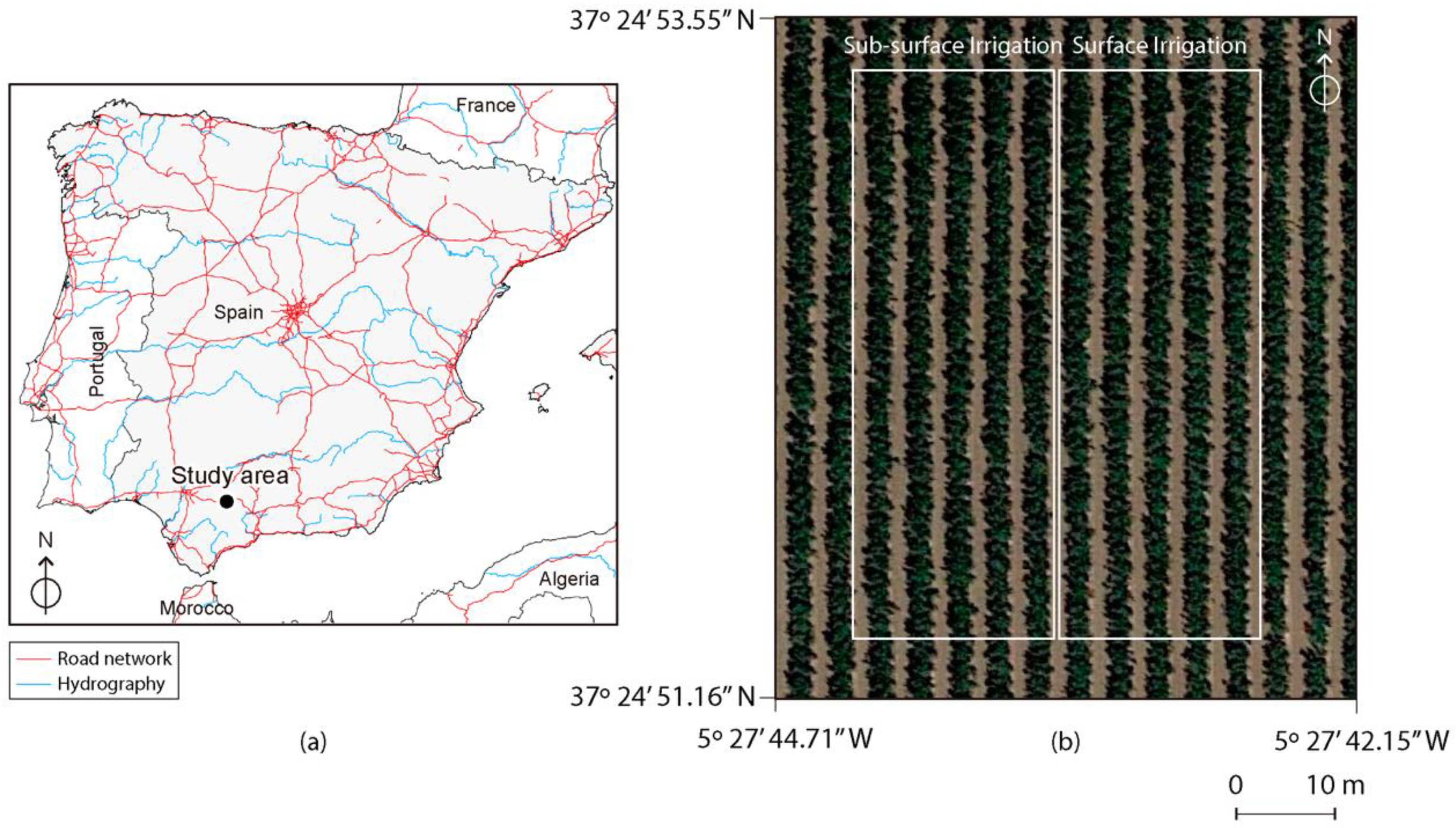
2.1. Study Area and UAV Flights

The study site was located in Marchena (Seville province, Spain) (37°24′52.7″ N, 5°27′44.9″ W, WGS84) (Figure 2a) in a 7-ha commercial orchard planted in 2015 with the olive cultivar Arbequina at a spacing of 3 m × 1.5 m (Figure 2b). The hedgerow orchard was adapted in equal parts to DI or SDI with carry self-compensating dripper pipes at 2.2 L/h spaced 0.5 m apart along the irrigation line and placed 0.5 m from the trunks and, in the case of SDI, buried 0.45 m deep. The trees were irrigated weekly with the seasonal water amount equivalent to 100% of ETc. Soil properties and agricultural practices were similar in both areas where the irrigation systems were implemented. The climate is Mediterranean with an average annual temperature and precipitation (concentrated mostly in late fall and winter) of 18.8 °C and 544 mm, respectively. A representative area including 413 olive trees (200 olives trees irrigated with DI and 213 with SDI) was used for data analyses.

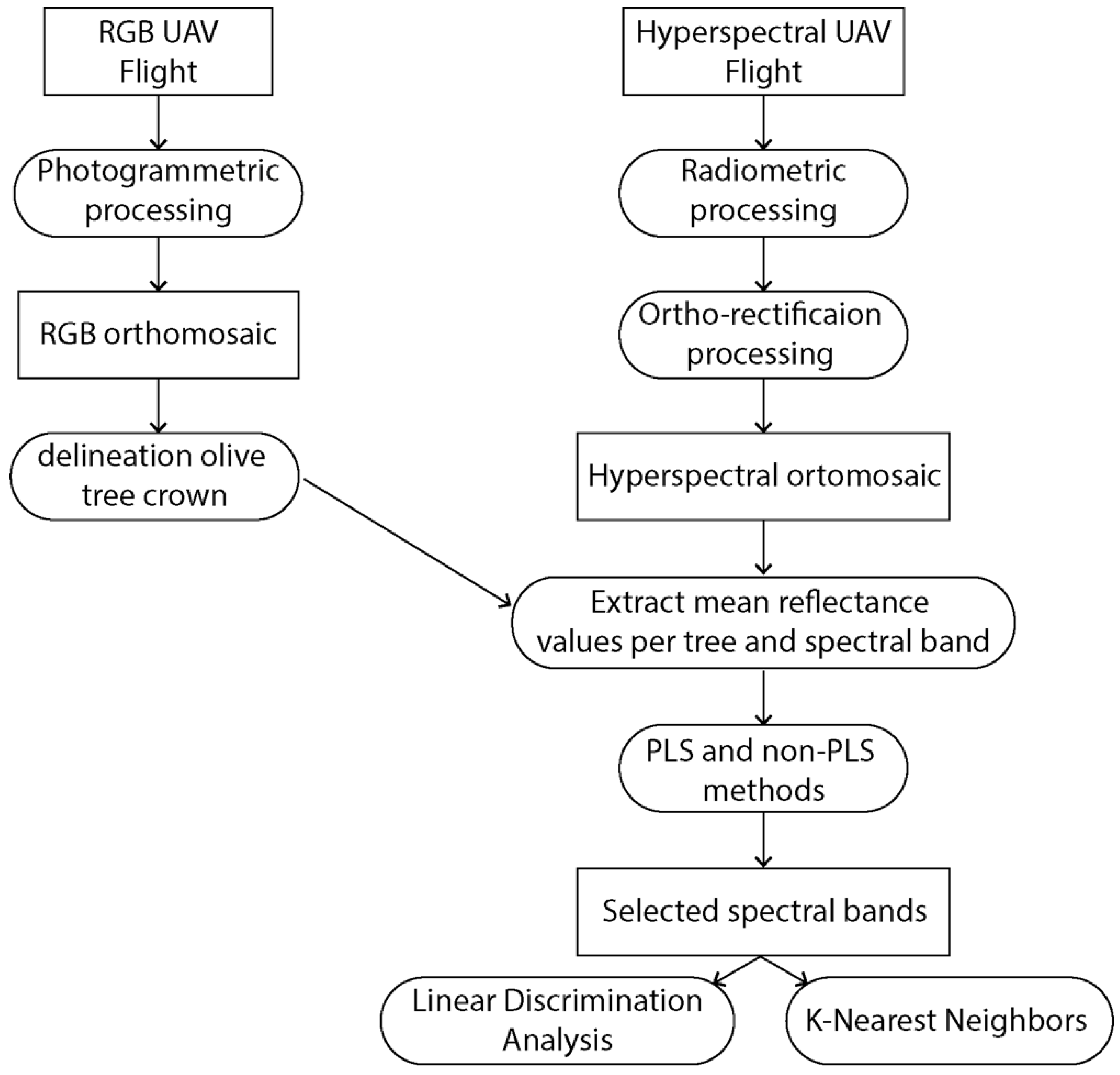
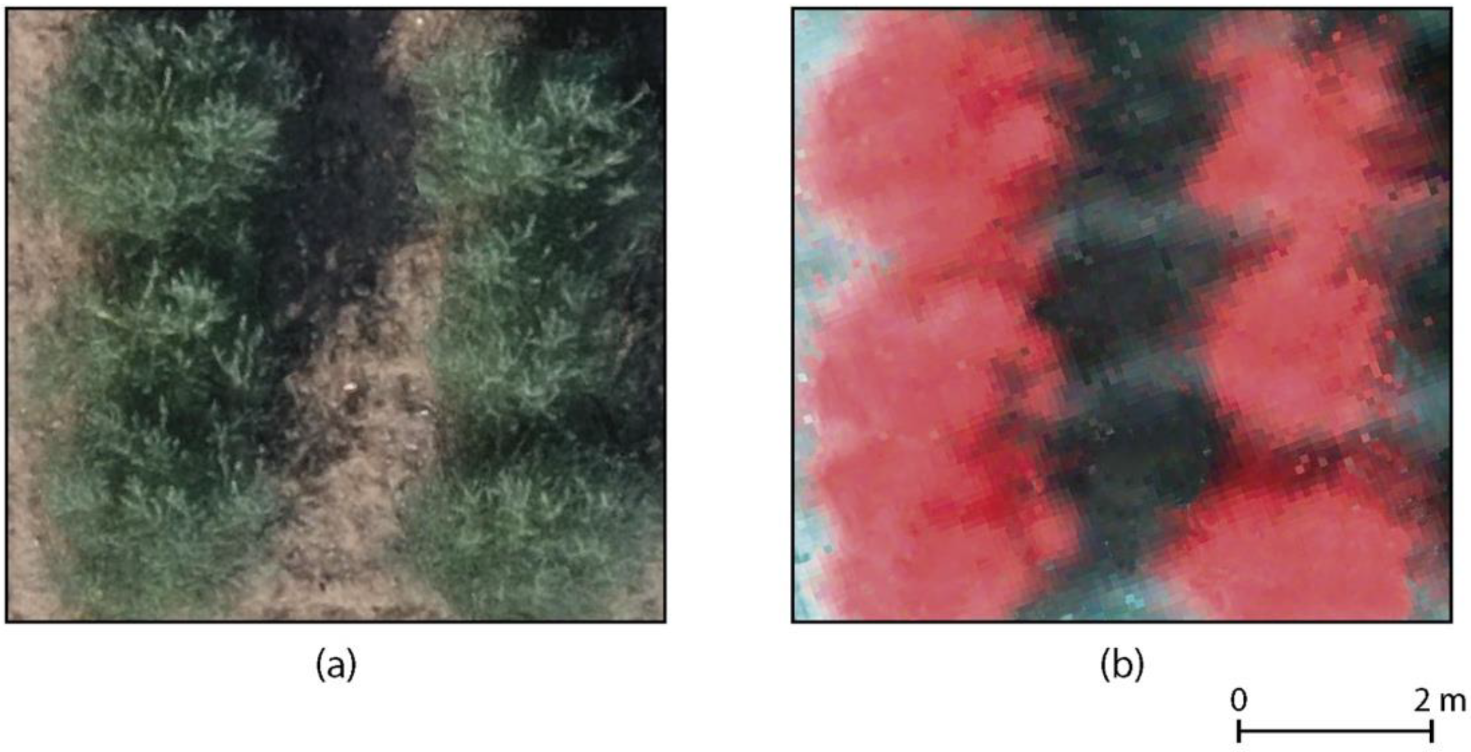
2.2. UAV Flights and Processing

Two UAV flights, RGB and hyperspectral, were performed on 22 May 2020 at solar noon to take advantage of the position of the sun and minimize shadows in the images acquired. The RGB UAV flight was used to precisely delineate each of the olive trees in the study area while the hyperspectral UAV flight characterized each of them spectrally. A DJI Mavic Pro 2 (SZ DJI Technology Co., Shenzhen, China) was used to perform the RGB flight. As the payload, a Hasselblad L1D-20c (Hasselblad Group, Göteborg, Sweden) was used, which provides an image of 13.2 mm × 8.8 mm, a focal length of 10.3 mm and an image size of 5472 × 3648 pixels. This UAV was flown at an altitude of 65 m above ground level (AGL) and forward and side-lap were 80% and 70%, respectively. Ground Sample Distance (GSD) was 1.6 cm taking into account the characteristics of the sensor. For the hyperspectral flight, a DJI Matrice 600 Pro (SZ DJI Technology Co., Shenzhen, China) was used. This UAV platform was also equipped with a Nano Hyperspec sensor (Headwall Photonics Inc., Boston, MA, USA) with 270 spectral bands (6-nm FWHM) both in the VNIR spectral range (400–1000 nm) with a sampling of 2.2 nm. Being a push-broom sensor, imagery is collected, line by line, at 12-bit radiometric resolution along the flight path where each line of pixels comprises 640 spatial pixels. The hyperspectral sensor was mounted on a Ronin-MX gimbal system (SZ DJI Technology Co., Shenzhen, China) to minimize external disturbances such as roll, pitch and yaw oscillations. This UAV platform was flown at an altitude of 100 m AGL, GSD being equal to 6 cm taking into account the characteristic of the sensor.

Prior to the UAV flights, five artificial targets were placed in the study area as Ground Control Points (GCPs), one in each corner and the other in the center. Each GCP was measured with the stop-and-go technique through relative positioning by means of the NTRIP protocol (The Radio Technical Commission for Maritime Services, RTCM, for Networked Transfer via Internet Protocol) using two GNSS (Global Navigation Satellite System) receivers. One of the receivers was a reference station for the GNSS Red Andaluza de Posicionamiento (RAP) network from the Institute of Statistics and Cartography of Andalusia, Spain, and the other, a Leica GS15 GNSS (Leica Geosystems AG, Heerbrugg, Switzerland), functioned as the rover receiver. In addition, a known reflectance value calibration tarp was placed in the center of the plot to subsequently correct the spectral cubes radiometrically. Before the hyperspectral UAV flight, the sensor capture mode was configured to set up the number of frames per second in accordance with the flight speed and AGL flight height. Likewise, the exposure level was established through the determination of the reflectance curve of a 90% target in order to avoid saturating the sensor in the recording of the spectral cubes. In addition, black body spectral information was taken by closing the aperture to later convert the digital levels to radiance values.

To produce an RGB orthomosaic from the RGB UAV flight, photogrammetric processing was divided into four stages: aerial triangulation, Digital Surface Model (DSM) generation, rectification of individual images and orthomosaicking. Aerial triangulation determined the individual external orientation of each image of the photogrammetric block. Afterwards, a dense point cloud was generated using Structure from Motion (SfM) techniques [88] to create a DSM. Finally, individual images were rectified and mosaicked to generate an RGB UAV orthomosaic of the study area. This methodology has been validated in previous research projects [19,89,90] and was performed using Pix4Dmapper (Pix4D S.A., Prilly, Switzerland). The hyperspectral data processing was divided into three stages [91]. Firstly, each hyperspectral cube was converted from digital number to radiance values, using dark reference captured prior to the UAV flight. Secondly, radiance values were converted to reflectance values using the values from the calibration tarp. Finally, all the reflectance hyperspectral cubes were orthorectified using data from the GNSS receivers, the Inertial Measurement Unit (IMU) and the Shuttle Radar Topography Mission (SRTM) Digital Elevation Model [92]. The accuracy and spatial resolution of the SRTM model was adequate due to the smooth relief of the study area. This processing was performed using SpectralView software (Headwall Photonics Inc., Boston, MA, USA).

Due to the difficulty in segmenting individual trees, an RGB orthomosaic was used to manually digitize polygons of all the olive trees, using the QGIS desktop Geographic Information System. As an example, a partial view of the hedgerow in the RGB and hyperspectral orthomosaic is shown in Figure 3. Then, for each olive tree, the mean spectral reflectance value for each of the 270 spectral bands was calculated, generating a spectral curve at the canopy level. This step was automated using a script developed in the Python programming language [93].

2.3. Wavelength Selection Methods Used and Evaluation

Although there are other methods, this project focused on applying those methods that use the output of a PLS algorithm to identify a subset of important variables. As such, the variables analyzed in this project were the wavelengths registered by the hyperspectral sensor. The PLS selection methods used in this study are grouped by category (

Table 1. Evaluated wavelength selection PLS methods.

Category	PLS Method	Reference
Filter	Loading Weights (LW-PLS)	[68]
	Regression Coefficient (RC-PLS)	[69]
	Variable Importance in Projection (VIP-PLS)	[70]
Wrapper	Genetic Algorithm (GA-PLS)	[71]
	Uninformative Variable Elimination (UVE-PLS)	[72]
	Backward Variable Elimination (BVE-PLS)	[73]
	Subwindow Permutation Analysis (SwPA-PLS)	[74]
	Iterative Predictive Weighting (IPW-PLS)	[75]
	Regularized Elimination Procedure (REP-PLS)	[67]
	Backward Interval (BiPLS)	[76]
	Forward Interval (FiPLS)	[77]
	Competitive Adaptive Reweighted Sampling (CARS-PLS)	[78]
Embedded	Sparse (S-PLS)	[80]

). More information on the PLS methods used in this study can be found in the work by Mehmood et al. [67].

Other wavelength selection methods, such as the Least Absolute Shrinkage and Selection Operator (Lasso) and Boruta algorithms, were also included in this study [94,95]. Lasso can handle ill-posed problems (i.e., a large number of correlated variables compared to sample size) and works by penalizing the magnitude of the characteristic coefficients along with minimizing the error between the predicted and actual observations [96]. On the other hand, the Boruta algorithm was developed to identify all relevant variables within a classification framework [97]. This method searches for relevant characteristics by comparing the importance of the original attributes with the importance that can be obtained at random, estimated using their permuted copies, and progressively eliminating irrelevant characteristics to stabilize the test. First, the dataset is duplicated, and the values are shuffled in each column; these are called shadow characteristics. Then, a classifier is trained on the dataset to extract the importance of each characteristic. Random Forest is one of the most widely used classifiers for this purpose [97]. As a final step, a combined analysis was performed considering the individual results from all the PLS, Lasso and Boruta methods used, which has been termed the All-together method.

2.4. Evaluation of Wavelength Selection Methods

LDA and KNN were applied to classify irrigation techniques used in each olive tree. Of the total number of olive trees, 75% were used in the calibration phase (explained below) and 25% for prediction (

Table 2. Number of samples per irrigation technique for calibration and prediction set.

	Sub-Surface Irrigation	Surface Irrigation
Calibration set	160	150
Prediction set	53	50
Total	213	200

). Before applying LDA or KNN classification, the dataset was divided into two smaller datasets that were used for calibration and prediction purposes. The calibration subset of data was used to estimate the parameters of the classifier model and the prediction subset of data was used to check the results of the model. Calibration and prediction were performed following an iterative process where subsets of data changed per iteration.

Overall accuracy (OA) of LDA and KNN results were calculated by summing the number of correctly classified olive trees and dividing by the total number of trees. Moreover, the accuracy of each irrigation technique was evaluated [98]. In addition, efficiency of methods applied were calculated in the prediction stage. According to Xia et al. [87], the efficiency of a wavelength selection method is based on the prediction rate and the number of variables, being calculated as follows:

$$E=\frac{\left(D_s-D_f\right)\times \left(N_f-N_s\right)}{N_f}\times 100$$

(1)

where E is the efficiency of the wavelength selection method evaluated, D_s is the OA obtained by a PLS method, D_f is the OA obtained using all wavelengths registered by the UAV hyperspectral sensor, N_f is the total number of wavelengths and N_s is the number of wavelengths selected by the method used. If E is higher than or equal to 0.5, the selection method is highly efficient. On the other hand, if E ranges from −0.5 to 0.5 the method is shown to be efficient, except if E is equal to 0 and $\left(N_f-N_s\right)/N_f$ is greater than or equal to 0.8, indicating the method to be highly efficient. Finally, if E is less than or equal to −0.5 the method is of low efficiency.

2.5. Software

LW-PLS, RC-PLS, VIP-PLS, AG-PLS, UVE-PLS, BVE-PLS, SwPA-PLS, IPW-PLS, REP-PLS, BiPLS, FiPLS, CARS-PLS, S-PLS, Lasso and Boruta were conducted within the R software environment [99] using RStudio [100], with the packages shown in

Table 3. R packages used for wavelength selection methods.

PLS Method	R Packages	Reference
Loading Weights (LW-PLS)	plsVarSel, pls	[67,101]
Regression Coefficient (RC-PLS)	plsVarSel, pls, threshr	[67,101,102]
Variable Importance in Projection (VIP-PLS)	plsVarSel, pls	[67,101]
Genetic Algorithm (GA-PLS)	plsVarSel	[67]
Uninformative Variable Elimination (UVE-PLS)	plsVarSel	[67]
Backward Variable Elimination (BVE-PLS)	plsVarSel	[67]
Subwindow Permutation Analysis (SwPA-PLS)	plsVarSel	[67]
Iterative Predictive Weighting (IPW-PLS)	plsVarSel	[67]
Regularized Elimination Procedure (REP-PLS)	plsVarSel	[67]
Backward Interval (BiPLS)	mdatools	[103]
Forward Interval (FiPLS)	mdatools	[103]
Competitive Adaptive Reweighted Sampling (CARS-PLS)	libPLSn	[104]
Sparse (S-PLS)	spls	[105]
Lasso	glmnet	[106]
Boruta	Boruta	[97]

. For the evaluation of the identification, linear and nonlinear techniques were established through LDA and KNN, respectively. The implementation of these algorithms was performed in Python [93] using the Scikit-learn library [84].

3. Results and Discussion

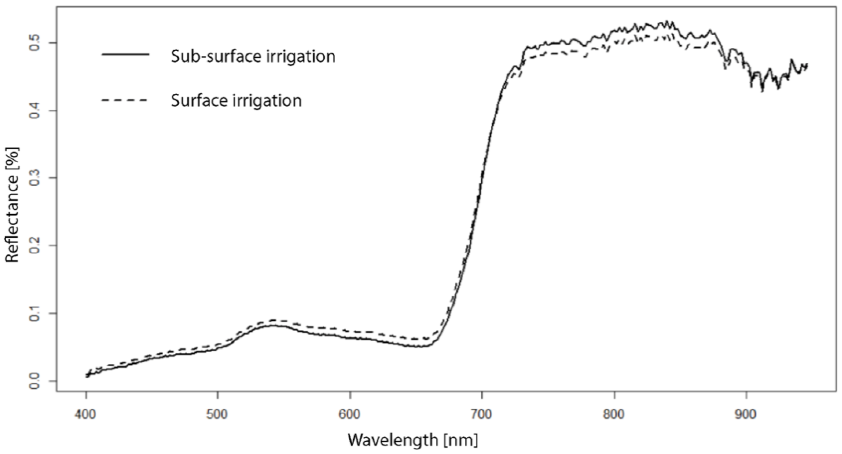
3.1. Spectral Reflectance Data

The mean spectral reflectance curves of olive trees, being irrigated with SDI or DI systems, were similar to the results obtained in related studies [107] (Figure 4). No differences were observed in the 400–550 and 880–947 nm ranges. However, different magnitudes of spectral reflectance were found in the 550–880 nm range. Therefore, within that range, there are 165 possible wavelengths to differentiate between both irrigation techniques. Given this high number, different wavelength selection methods, detailed above, were applied to identify those that best classify both types of irrigation.

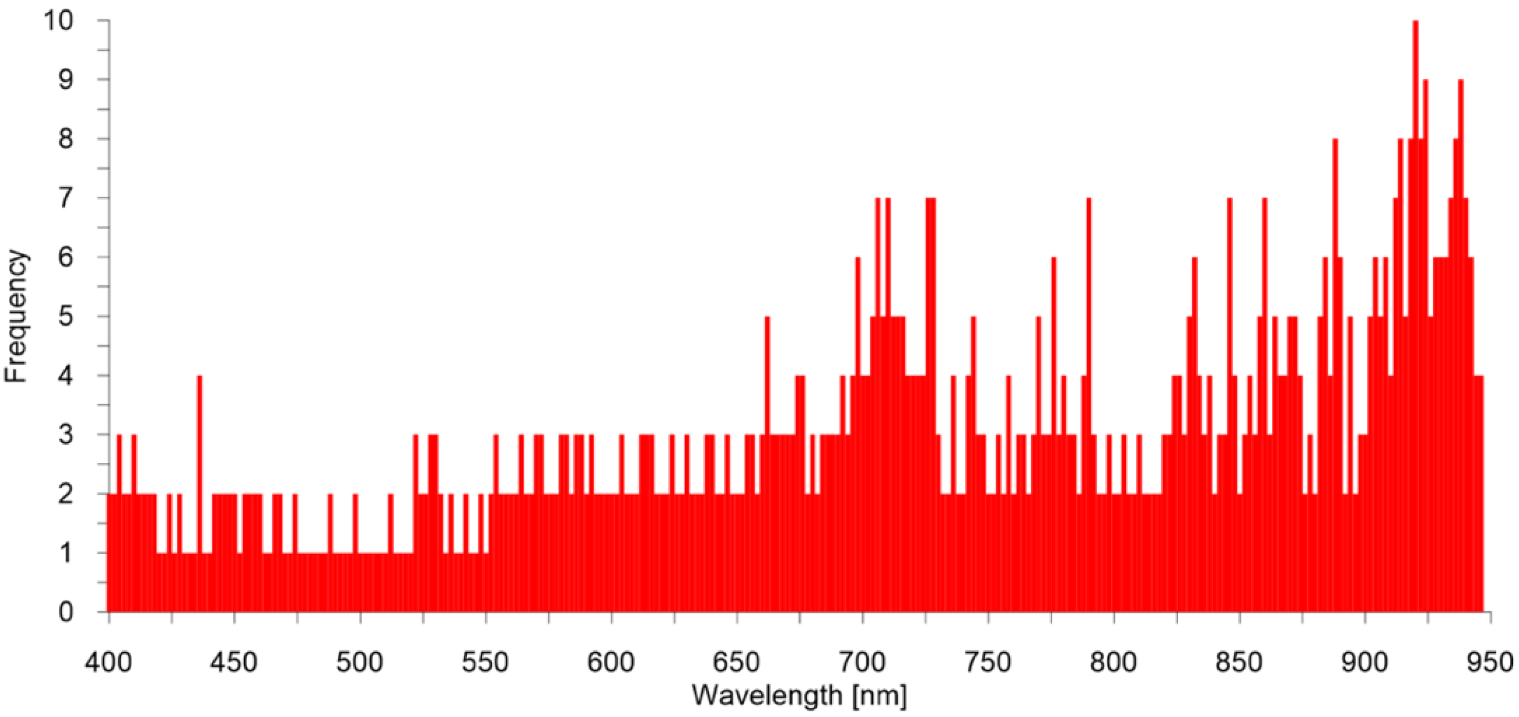
3.2. Wavelength Selection Results

The results of the application of the methods used, including the number of the selected wavelengths as well as their wavelengths, are shown in

Table 4. Wavelengths selected by different methods.

Method	Number of Wavelengths	Wavelengths [nm]
LW-PLS	5	882, 884, 890, 934, 942
RC-PLS	12	726, 728, 888, 904–908, 914, 920, 924, 928, 930–942
VIP-PLS	10	726, 888, 904, 906, 914, 924, 928, 936, 938, 942
GA-PLS	31	424, 428, 436, 442, 444, 458, 460, 522, 588, 612, 630, 640, 662, 698, 714, 716, 744, 758, 770, 780, 826, 846, 854, 860, 870, 878, 888, 912, 918, 920, 938
UVE-PLS	10	428, 696, 698, 700–704, 734, 792, 812, 856
BVE-PLS	69	686–734, 746, 776, 790, 840, 846, 848, 858, 860, 864–870, 880–890, 894–946
SwPA-PLS	77	410, 414, 418, 424, 436, 450, 466, 476, 490, 494, 496, 500, 506, 508, 518, 530–538, 542, 558, 562, 568, 576–580, 584, 588, 596, 612, 622–630, 640, 646, 648, 660, 668, 690, 702–706, 728, 738, 746, 752, 756, 768, 774, 782, 786, 804, 812, 822, 828, 836, 838, 848, 850, 856, 858, 860, 862, 874, 878, 882, 888, 896, 900, 904, 910, 914, 926, 936, 940
IPW-PLS	12	710, 790, 832, 846, 888, 914, 920–924, 936–940
REP-PLS	31	726, 728, 882, 884, 888, 890, 894, 898, 902–946
BiPLS	265	400–604, 624–946
FiPLS	54	660–676, 696–730, 768–784, 858–874, 912–928
CARS	2	436, 790
S-PLS	192	560–714, 720–946
Lasso	17	404, 662, 698, 704, 788, 844, 846, 858, 886, 904, 912, 918–922, 934–938
Boruta	29	430, 456, 464, 474, 636, 638, 644, 646, 650–660, 698, 774, 776, 780, 792, 794, 810, 816, 818, 838, 866, 868, 914, 930, 936
All-together	18	790, 814, 846, 860, 866, 868, 870, 882, 888, 892, 898, 902, 904, 920, 928, 934, 936, 940

. Depending on the method employed, the number of wavelengths varied considerably. The method that selected the least number of wavelengths was CARS, followed by LW-PLS, neither exceeding five wavelengths, less than 1% of the original wavelengths registered. A set of methods (RC-PLS, VIP-PLS and IPW-PLS) selected a range of 10 wavelengths, equal to 3.6% of the original wavelength number, and others selected 17–77 (6.2–28.1%) wavelengths (GA-PLS, BVE-PLS, SwPA-PLS, REP_PLS, FiPLS, Lasso and Boruta). Finally, the S-PLS and BiPLS methods were the ones that selected the largest number of wavelengths, 192 (70%) and 265 (96.7%), respectively. As such, the reduction in the number of wavelengths of interest will be higher or lower depending on the method used.

The total number of times a wavelength was selected by the total number of methods simultaneously employed is shown in Figure 5. Although there was a difference in the spectrum of SDI and DI in the wavelengths of around 600–650 nm (Figure 4), the frequency of selection by the selection methods employed in this range was low (Figure 5). Of all the methods applied, 18 wavelengths were selected by almost half the methods (All-together method; Table 4). All within the infrared region and for a total of nine times, the wavelength 920 nm was selected the most to predict the irrigation method used in this study. The utility of the All-together method was demonstrated for investigating agricultural features using hyperspectral imagery.

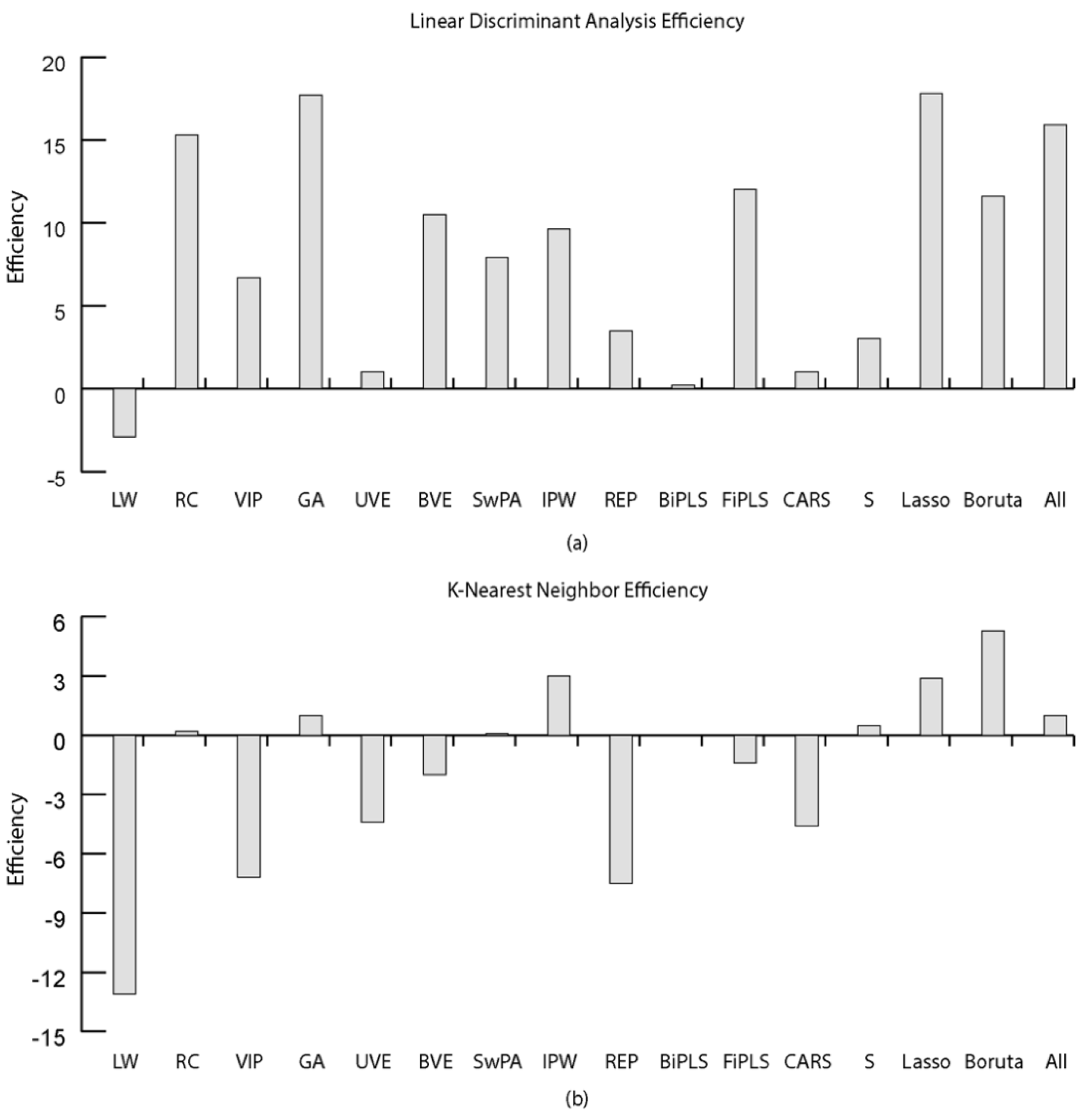
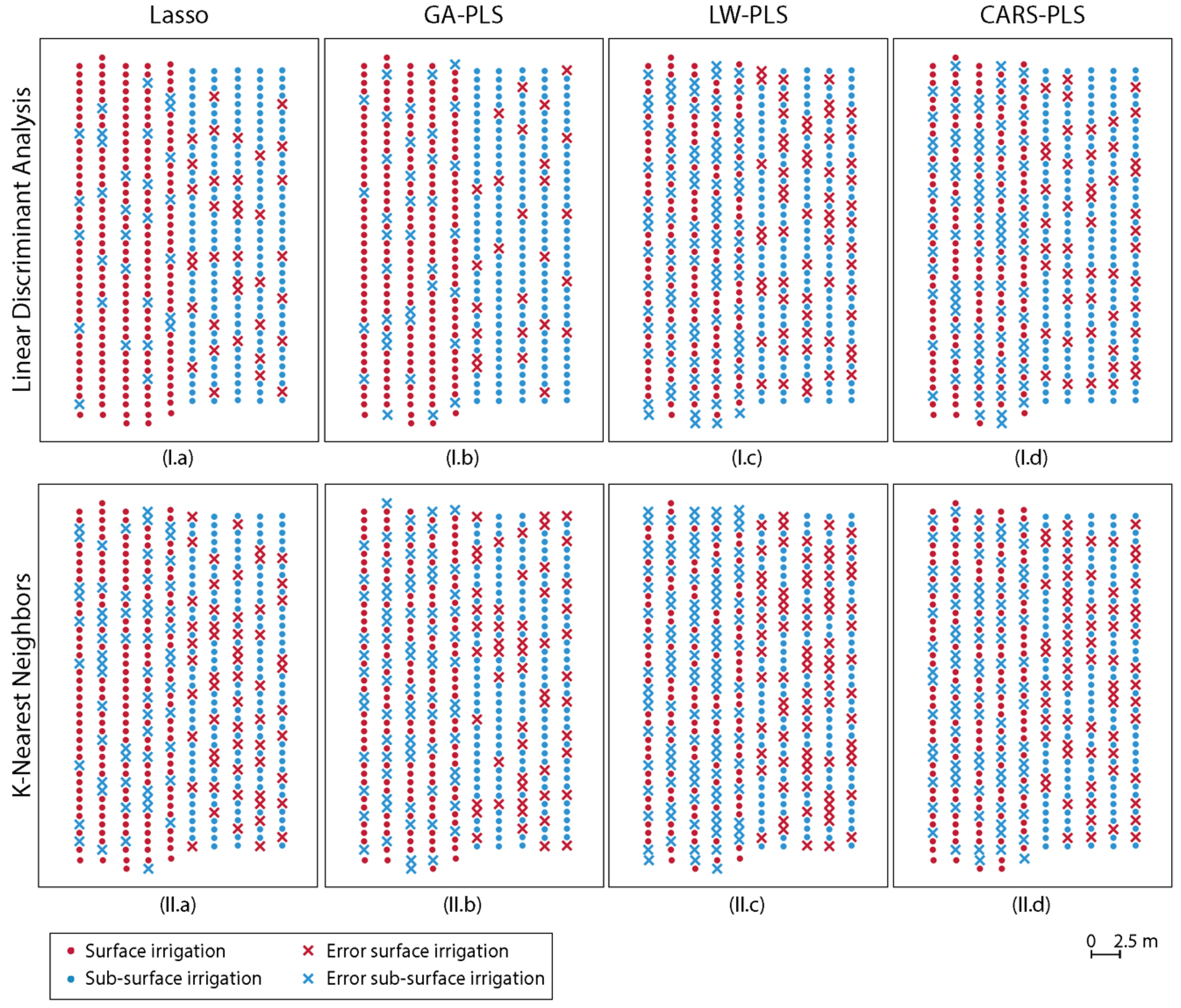
3.3. Quality and Efficiency of Classification with Each Selection Method

The accuracy and efficiency results of the irrigation technique rating using LDA and KNN methods and their efficiency are shown in

Table 5. Overall accuracy (OA), Accuracy of Sub-Surface drip irrigation (A SDI), Accuracy of Surface drip irrigation (A DI) and Efficiency (E) results of Linear Discriminant Analysis (LDA) and K-Nearest Neighbors (KNN) using different selection methods.

	LDA				KNN
Method	OA (%)	A SDI (%)	A DI (%)	E	OA (%)	A SDI (%)	A DI (%)	E
All bands	65.0	62.5	68.7	-	68.1	64.6	73.6	-
LW-PLS	62.5	57.5	70.7	−2.9	54.8	51.7	61.1	−13.1
RC-PLS	81.3	80.7	81.1	15.3	68.3	64.4	73.3	0.2
VIP-PLS	72.2	69.5	73.3	6.7	60.6	55.1	71.9	−7.2
GA-PLS	85.2	83.6	87.6	17.7	69.2	65.4	73.0	1.0
UVE-PLS	66.5	61.9	72.8	1.0	63.5	59.9	70.1	−4.4
BVE-PLS	79.0	78.5	79.5	10.5	65.4	61.7	71.1	−2.0
SwPA-PLS	76.3	76.2	76.4	7.9	68.3	66.6	70.0	0.1
IPW-PLS	75.5	71.5	79.5	9.6	71.2	67.4	75.4	3.0
REP-PLS	69.3	67.9	71.3	3.5	59.6	54.5	71.1	−7.5
BiPLS	70.2	68.3	72.1	0.2	69.2	64.2	75.2	0.0
FiPLS	80.1	81.6	79.0	12.0	66.3	63.5	70.1	−1.4
CARS	66.0	60.1	76.1	1.0	63.5	60.1	67.9	−4.6
S-PLS	75.3	75.3	75.3	3.0	69.2	66.2	72.2	0.5
Lasso	84.0	86.4	82.3	17.8	71.2	72.3	72.2	2.9
Boruta	78.0	76.4	80.2	11.6	74.0	73.5	75.6	5.3
All-together	82.5	78.6	85.3	15.9	69.2	65.3	74.9	1.0

, while Figure 6 shows their efficiency. In general terms, LDA classifications showed better overall accuracy than KNN, in both calibration and prediction. Considering LDA, overall accuracy prediction (OAP) using all wavelengths was equal to 65%. Using only those selected wavelengths from a selection method, OAP improved, except in LW-PLS, the mean OPA being equal to 75%. The highest percentage of improvement was offered by GA-PLS, at 20%, while the lowest was offered by CARS, at 1%. In addition, ten of the methods evaluated improved the predictive quality of the irrigation technique by more than 10% (RC-PLS, GA-PLS, BVE-PLS, SwPA-PLS, IPW-PLS, BiPLS, S-PLS, Lasso, Boruta and All-together). On the other hand, the OAP applying KNN using all wavelengths was equal to 68.1% while just using the wavelengths selected by a PLS method generally resulted in a slightly lower OAP, with a mean value equal to 66.4%. Boruta was the method that showed the highest percentage of improvement, with an OAP of 74%. In total, seven of the methods offered an improvement in irrigation system prediction (GA-PLS, IPW-PLS, BiPLS, S-PLS, Lasso, Boruta and All-together). In addition, while LDA showed similar accuracy classifying both irrigation techniques, KNN offered worse results with the SDI technique.

While LDA offered better results than KNN, all the methods used were highly efficient except for LW-PLS (Figure 6). GA-PLS and Lasso scored the highest with an efficiency equal to 17.7 and 17.8, respectively (Figure 6a). In contrast, only six of the sixteen methods were highly efficient using KNN, Boruta being the most efficient with a value equal to 5.3 (Figure 6b). In addition, the irrigation classification maps of some of the selection methods assessed are shown in Figure 7. From a visual analysis, no spatial correlation was detected in the errors obtained as well as the presence of a higher concentration of errors in the perimeter of each type of irrigation.

Although combining bands when using hyperspectral data for olive trees is common [108], this study shows that the use of individual wavelengths could be an interesting and more accessible way to manage hyperspectral data. The results obtained from each selection method were different, showing methods that improved overall accuracy and efficiency in the classification of irrigation systems and methods that did not. This variation in the results obtained by selection methods were similar to those obtained by other authors [87]. In this study, according to the LDA and KNN results, GA-PLS, IPW-PLS, Lasso, Boruta and All-together methods were those which improved OAP while being highly efficient at the same time. In addition, RC-PLS and FiPLS methods showed a high overall accuracy using LDA. The GA-PLS method was also one of the most efficient, as seen by Xia et al. (2017) [87]. These authors found spectral differences between different samples of Ophiopogon japonicus from differing origins, using, in their case, an imaging spectrograph. In addition, although the Boruta method has not been widely used for the selection of variables in remote sensing or other disciplines, results obtained in this study show that it could be considered as a promising method for the selection of hyperspectral wavelengths. On the other hand, LW-PLS showed low efficiency and lower OAP. This can be explained because this method greatly reduces wavelengths and therefore eliminated useful information as indicated in other works [87]. The efficiency of RC-PLS, VIP-PLS, UVE-PLS, BVE-PLS, SwPA-PLS, REP-PLS, BiPLS, FiPLS, CARS-PLS and S-PLS varied depending on whether LDA or KNN was used. In general, LDA showed better classification results than KNN, which can be explained due to the fact that KNN needs to have large training data in order to achieve acceptable classification results, as indicated by Starzacher and Rinner (2008) [109].

In general, these preliminary results show the need to analyze the relationships between wavelengths registered by a hyperspectral sensor and the object of study to optimize the number of wavelengths utilized. As a future line of research, the analysis of which combinations of wavelengths may be of interest to characterize irrigated areas in more detail is proposed. In addition, other features such as soil properties or olive cultivars along with other classifiers should be considered for improving the characterization of irrigation areas.

4. Conclusions

This study explored the use of UAV hyperspectral reflectance measurements of olive trees as a means for differentiating irrigation systems. Because of the high dimension and multicollinearity of the data, selection methods were found appropriate due to their capacity to extract useful wavelengths for analyzing categorial data, even when using individualized wavelengths. The results showed how the spectral response of olive trees is sensitive to the irrigation technique used, allowing improved information for the mapping of irrigated areas. Overall accuracy in the classification of irrigation systems in olives trees using LDA and KNN ranged from 54.8% and 85.2%. These variations showed the need to select the appropriate wavelength selection method. In addition, LDA offered more accurate results than KNN. In our study, GA-PLS, RC-PLS, Lasso, FiPLS, Boruta and All-together showed an overall accuracy of 75% or higher. They were all highly efficient methods and resulted in an improved classification.

The study has shown how the use of hyperspectral UAV data allows the irrigated areas of olive groves to be characterized in greater detail. This will generate information of interest for decision-making processes in the context of water use policies, enabling better understanding of irrigated olive groves and improving the management of water resources.

References

1. Ozdogan, M.; Yang, Y.; Allez, G.; Cervantes, C. Remote sensing of irrigated agriculture: Opportunities and challenges. Remote Sens. 2010, 2, 2274–2304. [Google Scholar] [CrossRef] [Green Version]
2. Cai, X.; Rosegrant, M.W. Global Water Demand and Supply Projections: Part 1. A Modeling Approach. Water Int. 2002, 27, 159–169. [Google Scholar] [CrossRef]
3. Wisser, D.; Frolking, S.; Douglas, E.M.; Fekete, B.M.; Vörösmarty, C.J.; Schumann, A.H. Global irrigation water demand: Variability and uncertainties arising from agricultural and climate data sets. Geophys. Res. Lett. 2008, 35, 1–5. [Google Scholar] [CrossRef] [Green Version]
4. Kueppers, L.M.; Snyder, M.A.; Sloan, L.C. Irrigation cooling effect: Regional climate forcing by land-use change. Geophys. Res. Lett. 2007, 34, 1–5. [Google Scholar] [CrossRef] [Green Version]
5. Droogers, P.; Aerts, J. Adaptation strategies to climate change and climate variability: A comparative study between seven contrasting river basins. Phys. Chem. Earth 2005, 30, 339–346. [Google Scholar] [CrossRef] [Green Version]
6. Thenkabail, P.S.; Dheeravath, V.; Biradar, C.M.; Gangalakunta, O.R.P.; Noojipady, P.; Gurappa, C.; Velpuri, M.; Gumma, M.; Li, Y. Irrigated area maps and statistics of India using remote sensing and national statistics. Remote Sens. 2009, 1, 50–67. [Google Scholar] [CrossRef] [Green Version]
7. Escobar, R.F.; de la Rosa, R.; Leon, L.; Gomez, J.A.; Testi, F.; Orgaz, M.; Gil-Ribes, J.A.; Quesada-Moraga, E.; Trapero, A. Evolution and sustainability of the olive production systems. In Present and Future of the Mediterranean Olive Sector; CIHEAM/IOC: Zaragoza, Spain, 2013; Volume 106, pp. 11–41. ISBN 2-85352-512-0. [Google Scholar]
8. Martínez, J.; Reca, J. Water use efficiency of surface drip irrigation versus an alternative subsurface drip irrigation method. J. Irrig. Drain. Eng. 2014, 140, 1–9. [Google Scholar] [CrossRef]
9. Briggs, L.J.; Shantz, H.L. The water requirement of plants. In Bureau of Plant Industry Bulletin; Wiley: Akron, OH, USA, 1913; p. 96. [Google Scholar]
10. Yu, L.; Gao, X.; Zhao, X. Global synthesis of the impact of droughts on crops’ water-use efficiency (WUE): Towards both high WUE and productivity. Agric. Syst. 2020, 177, 102723. [Google Scholar] [CrossRef]
11. Tolk, J.; Howell, T.; Evett, S. Effect of mulch, irrigation, and soil type on water use and yield of maize. Soil Tillage Res. 1999, 50, 137–147. [Google Scholar] [CrossRef]
12. Basso, B.; Ritchie, J.T. Evapotranspiration in High-Yielding Maize and under Increased Vapor Pressure Deficit in the US Midwest. Agric. Environ. Lett. 2018, 3, 170039. [Google Scholar] [CrossRef]
13. Bota, J.; Tomás, M.; Flexas, J.; Medrano, H.; Escalona, J.M. Differences among grapevine cultivars in their stomatal behavior and water use efficiency under progressive water stress. Agric. Water Manag. 2016, 164, 91–99. [Google Scholar] [CrossRef]
14. Michelon, N.; Pennisi, G.; Myint, N.O.; Orsini, F.; Gianquinto, G. Strategies for improved Water Use Efficiency (WUE) of field-grown lettuce (Lactuca sativa L.) under a semi-arid climate. Agronomy 2020, 10, 668. [Google Scholar] [CrossRef]
15. Thenkabail, P.S.; Schull, M.; Turral, H. Ganges and Indus river basin land use/land cover (LULC) and irrigated area mapping using continuous streams of MODIS data. Remote Sens. Environ. 2005, 95, 317–341. [Google Scholar] [CrossRef]
16. Toureiro, C.; Serralheiro, R.; Shahidian, S.; Sousa, A. Irrigation management with remote sensing: Evaluating irrigation requirement for maize under Mediterranean climate condition. Agric. Water Manag. 2017, 184, 211–220. [Google Scholar] [CrossRef]
17. Gao, Q.; Zribi, M.; Escorihuela, M.J.; Baghdadi, N.; Segui, P.Q. Irrigation mapping using Sentinel-1 time series at field scale. Remote Sens. 2018, 10, 1495. [Google Scholar] [CrossRef] [Green Version]
18. Jalilvand, E.; Tajrishy, M.; Hashemi, S.A.G.Z.; Brocca, L. Quantification of irrigation water using remote sensing of soil moisture in a semi-arid region. Remote Sens. Environ. 2019, 231, 111226. [Google Scholar] [CrossRef]
19. Mesas-Carrascosa, F.-J.; Torres-Sánchez, J.; Clavero-Rumbao, I.; García-Ferrer, A.; Peña, J.-M.; Borra-Serrano, I.; López-Granados, F. Assessing Optimal Flight Parameters for Generating Accurate Multispectral Orthomosaicks by UAV to Support Site-Specific Crop Management. Remote Sens. 2015, 7, 12793–12814. [Google Scholar] [CrossRef] [Green Version]
20. Pageot, Y.; Baup, F.; Inglada, J.; Baghdadi, N.; Demarez, V. Detection of Irrigated and Rainfed Crops in Temperate Areas Using Sentinel-1 and Sentinel-2 Time Series. Remote Sens. 2020, 12, 3044. [Google Scholar] [CrossRef]
21. Velpuri, N.M.; Thenkabail, P.S.; Gumma, M.K.; Biradar, C.; Dheeravath, V.; Noojipady, P.; Yuanjie, L. Influence of resolution in irrigated area mapping and area estimation. Photogramm. Eng. Remote Sens. 2009, 75, 1383–1395. [Google Scholar] [CrossRef] [Green Version]
22. Matese, A.; Toscano, P.; Di Gennaro, S.F.; Genesio, L.; Vaccari, F.P.; Primicerio, J.; Belli, C.; Zaldei, A.; Bianconi, R.; Gioli, B. Intercomparison of UAV, aircraft and satellite remote sensing platforms for precision viticulture. Remote Sens. 2015, 7, 2971–2990. [Google Scholar] [CrossRef] [Green Version]
23. Eastman, J.R.; Sangermano, F.; Machado, E.A.; Rogan, J.; Anyamba, A. Global trends in seasonality of Normalized Difference Vegetation Index (NDVI), 1982–2011. Remote Sens. 2013, 5, 4799–4818. [Google Scholar] [CrossRef] [Green Version]
24. Berni, J.A.J.; Zarco-Tejada, P.J.; Suárez, L.; Fereres, E. Thermal and Narrowband Multispectral Remote Sensing for Vegetation Monitoring from an Unmanned Aerial Vehicle Improved Evapotranspiration using Unmanned Aerial Vehicles View project High throughput and remote trait measurement View project Thermal and Nar. IEEE Trans. Geosci. Remote Sens. 2009, 47, 722–738. [Google Scholar] [CrossRef] [Green Version]
25. Anderson, K.; Gaston, K.J. Lightweight unmanned aerial vehicles will revolutionize spatial ecology. Front. Ecol. Environ. 2013, 11, 138–146. [Google Scholar] [CrossRef] [Green Version]
26. Berra, E.F.; Gaulton, R.; Barr, S. Assessing spring phenology of a temperate woodland: A multiscale comparison of ground, unmanned aerial vehicle and Landsat satellite observations. Remote Sens. Environ. 2019, 223, 229–242. [Google Scholar] [CrossRef]
27. Jay, S.; Baret, F.; Dutartre, D.; Malatesta, G.; Héno, S.; Comar, A.; Weiss, M.; Maupas, F. Exploiting the centimeter resolution of UAV multispectral imagery to improve remote-sensing estimates of canopy structure and biochemistry in sugar beet crops. Remote Sens. Environ. 2019, 231, 110898. [Google Scholar] [CrossRef]
28. Radoglou-Grammatikis, P.; Sarigiannidis, P.; Lagkas, T.; Moscholios, I. A compilation of UAV applications for precision agriculture. Comput. Netw. 2020, 172, 107148. [Google Scholar] [CrossRef]
29. Nhamo, L.; van Dijk, R.; Magidi, J.; Wiberg, D.; Tshikolomo, K. Improving the accuracy of remotely sensed irrigated areas using post-classification enhancement through UAV capability. Remote Sens. 2018, 10, 712. [Google Scholar] [CrossRef] [Green Version]
30. Qin, J.; Chao, K.; Kim, M.S.; Lu, R.; Burks, T.F. Hyperspectral and multispectral imaging for evaluating food safety and quality. J. Food Eng. 2013, 118, 157–171. [Google Scholar] [CrossRef]
31. Park, B.; Lu, R. (Eds.) Hyperspectral Imaging Technology in Food and Agriculture; Springer US: New York, NY, USA, 2015; ISBN 9781493928354. [Google Scholar]
32. Adão, T.; Hruška, J.; Pádua, L.; Bessa, J.; Peres, E.; Morais, R.; Sousa, J.J. Hyperspectral imaging: A review on UAV-based sensors, data processing and applications for agriculture and forestry. Remote Sens. 2017, 9, 1110. [Google Scholar] [CrossRef] [Green Version]
33. Yu, F.H.; Xu, T.Y.; Du, W.; Ma, H.; Zhang, G.S.; Chen, C.L. Radiative transfer models (RTMs) for field phenotyping inversion of rice based on UAV hyperspectral remote sensing. Int. J. Agric. Biol. Eng. 2017, 10, 150–157. [Google Scholar] [CrossRef]
34. Yue, J.; Yang, G.; Li, C.; Li, Z.; Wang, Y.; Feng, H.; Xu, B. Estimation of Winter Wheat Above-Ground Biomass Using Unmanned Aerial Vehicle-Based Snapshot Hyperspectral Sensor and Crop Height Improved Models. Remote Sens. 2017, 9, 708. [Google Scholar] [CrossRef] [Green Version]
35. Akhtman, Y.; Golubeva, E.I.; Tutubalina, O.V.; Zimin, M. Application of hyperspectural images and ground data for precision farming. Geogr. Environ. Sustain. 2017, 10, 117–128. [Google Scholar] [CrossRef]
36. Bauer, M.E.; Daughtry, C.S.T.; Vanderbilt, V.C. Spectral-agronomic relationships of corn, soybean and wheat canopies. In Proceedings of the Signatures Spectrales D’objets En Teledetection, Avignon, France, 18–22 January 1981; pp. 261–272. [Google Scholar]
37. Bohnenkamp, D.; Behmann, J.; Mahlein, A.K. In-field detection of Yellow Rust in Wheat on the Ground Canopy and UAV Scale. Remote Sens. 2019, 11, 2495. [Google Scholar] [CrossRef] [Green Version]
38. Scherrer, B.; Sheppard, J.; Jha, P.; Shaw, J.A. Hyperspectral imaging and neural networks to classify herbicide-resistant weeds. J. Appl. Remote Sens. 2019, 13, 044516. [Google Scholar] [CrossRef]
39. Rinaldi, M.; Castrignanò, A.; De Benedetto, D.; Sollitto, D.; Ruggieri, S.; Garofalo, P.; Santoro, F.; Figorito, B.; Gualano, S.; Tamborrino, R. Discrimination of tomato plants under different irrigation regimes: Analysis of hyperspectral sensor data. Environmetrics 2015, 26, 77–88. [Google Scholar] [CrossRef]
40. Renzullo, L.J.; Blanchfield, A.L.; Powell, K.S. A method of wavelength selection and spectral discrimination of hyperspectral reflectance spectrometry. IEEE Trans. Geosci. Remote Sens. 2006, 44, 1986–1994. [Google Scholar] [CrossRef]
41. Lu, B.; Dao, P.D.; Liu, J.; He, Y.; Shang, J. Recent Advances of Hyperspectral Imaging Technology and Applications in Agriculture. Remote Sens. 2020, 12, 2659. [Google Scholar] [CrossRef]
42. Thenkabail, P.S.; Enclona, E.A.; Ashton, M.S.; Van Der Meer, B. Accuracy assessments of hyperspectral waveband performance for vegetation analysis applications. Remote Sens. Environ. 2004, 91, 354–376. [Google Scholar] [CrossRef]
43. Becker, B.L.; Lusch, D.P.; Qi, J. Identifying optimal spectral bands from in situ measurements of Great Lakes coastal wetlands using second-derivative analysis. Remote Sens. Environ. 2005, 97, 238–248. [Google Scholar] [CrossRef]
44. Pu, R.; Gong, P.; Biging, G.S.; Larrieu, M.R. Extraction of red edge optical parameters from hyperion data for estimation of forest leaf area index. IEEE Trans. Geosci. Remote Sens. 2003, 41, 916–921. [Google Scholar] [CrossRef] [Green Version]
45. Darvishzadeh, R.; Atzberger, C.; Skidmore, A.K.; Abkar, A.A. Leaf Area Index derivation from hyperspectral vegetation indicesand the red edge position. Int. J. Remote Sens. 2009, 30, 6199–6218. [Google Scholar] [CrossRef]
46. Haboudane, D.; Miller, J.R.; Pattey, E.; Zarco-Tejada, P.J.; Strachan, I.B. Hyperspectral vegetation indices and novel algorithms for predicting green LAI of crop canopies: Modeling and validation in the context of precision agriculture. Remote Sens. Environ. 2004, 90, 337–352. [Google Scholar] [CrossRef]
47. Farrell, M.D.; Mersereau, R.M. On the impact of PCA dimension reduction for hyperspectral detection of difficult targets. IEEE Geosci. Remote Sens. Lett. 2005, 2, 192–195. [Google Scholar] [CrossRef]
48. Koonsanit, K.; Jaruskulchai, C.; Eiumnoh, A. Band Selection for Dimension Reduction in Hyper Spectral Image Using Integrated InformationGain and Principal Components Analysis Technique. Int. J. Mach. Learn. Comput. 2012, 2, 248–251. [Google Scholar] [CrossRef]
49. Burger, J.; Gowen, A. Data handling in hyperspectral image analysis. Chemom. Intell. Lab. Syst. 2011, 108, 13–22. [Google Scholar] [CrossRef]
50. Gao, L.; Zhao, B.; Jia, X.; Liao, W.; Zhang, B. Optimized kernel minimum noise fraction transformation for hyperspectral image classification. Remote Sens. 2017, 9, 548. [Google Scholar] [CrossRef] [Green Version]
51. Menon, V.; Du, Q.; Fowler, J.E. Fast SVD with Random Hadamard Projection for Hyperspectral Dimensionality Reduction. IEEE Geosci. Remote Sens. Lett. 2016, 13, 1275–1279. [Google Scholar] [CrossRef]
52. Fordellone, M.; Bellincontro, A.; Mencarelli, F. Partial least squares discriminant analysis: A dimensionality reduction method to classify hyperspectral data. Stat. Appl. Ital. J. Appl. Stat. 2018, 31, 181–200. [Google Scholar] [CrossRef]
53. Krishnan, A.; Williams, L.J.; McIntosh, A.R.; Abdi, H. Partial Least Squares (PLS) methods for neuroimaging: A tutorial and review. Neuroimage 2011, 56, 455–475. [Google Scholar] [CrossRef]
54. Ray, S.S.; Das, G.; Singh, J.P.; Panigrahy, S. Evaluation of hyperspectral indices for LAI estimation and discrimination of potato crop under different irrigation treatments. Int. J. Remote Sens. 2006, 27, 5373–5387. [Google Scholar] [CrossRef]
55. Mehmood, T.; Sæbø, S.; Liland, K.H. Comparison of variable selection methods in partial least squares regression. J. Chemom. 2020, 34. [Google Scholar] [CrossRef] [Green Version]
56. Abdi, H. Partial least squares regression and projection on latent structure regression (PLS Regression). WIREs Comput. Stat. 2010, 2, 97–106. [Google Scholar] [CrossRef]
57. Lu, B.; He, Y. Evaluating empirical regression, machine learning, and radiative transfer modelling for estimating vegetation chlorophyll content using bi-seasonal hyperspectral images. Remote Sens. 2019, 11, 1979. [Google Scholar] [CrossRef] [Green Version]
58. Thenkabail, P.S.; Mariotto, I.; Gumma, M.K.; Middleton, E.M.; Landis, D.R.; Huemmrich, K.F. Selection of hyperspectral narrowbands (hnbs) and composition of hyperspectral twoband vegetation indices (HVIS) for biophysical characterization and discrimination of crop types using field reflectance and hyperion/EO-1 data. IEEE J. Sel. Top. Appl. Earth Obs. Remote Sens. 2013, 6, 427–439. [Google Scholar] [CrossRef] [Green Version]
59. Thenkabail, P.S.; Smith, R.B.; De Pauw, E. Hyperspectral Vegetation Indices and Their Relationships with Agricultural Crop Characteristics. Remote Sens. Environ. 2000, 71, 158–182. [Google Scholar] [CrossRef]
60. Thenkabail, P.; Lyon, J. (Eds.) Hyperspectral Remote Sensing of Vegetation; CRC Press: Boca Raton, FL, USA, 2012. [Google Scholar]
61. Durif, G.; Modolo, L.; Michaelsson, J.; Mold, J.E.; Lambert-Lacroix, S.; Picard, F. High dimensional classification with combined adaptive sparse PLS and logistic regression. Bioinformatics 2018, 34, 485–493. [Google Scholar] [CrossRef]
62. Deb, D.; Mackey, D.; Opiyo, S.O.; McDowell, J.M. Application of alignment-free bioinformatics methods to identify an oomycete protein with structural and functional similarity to the bacterial AvrE effector protein. PLoS ONE 2018, 13, 1–19. [Google Scholar] [CrossRef] [Green Version]
63. Sampaio, P.S.; Soares, A.; Castanho, A.; Almeida, A.S.; Oliveira, J.; Brites, C. Optimization of rice amylose determination by NIR-spectroscopy using PLS chemometrics algorithms. Food Chem. 2018, 242, 196–204. [Google Scholar] [CrossRef]
64. Li, J.; Tong, Y.; Guan, L.; Wu, S.; Li, D. Optimization of COD determination by UV–vis spectroscopy using PLS chemometrics algorithms. Optik 2018, 174, 591–599. [Google Scholar] [CrossRef]
65. Luedeling, E.; Gassner, A. Partial Least Squares Regression for analyzing walnut phenology in California. Agric. For. Meteorol. 2012, 158–159, 43–52. [Google Scholar] [CrossRef]
66. Song, S.; Gong, W.; Zhu, B.; Huang, X. Wavelength selection and spectral discrimination for paddy rice, with laboratory measurements of hyperspectral leaf reflectance Shalei. ISPRS J. Photogramm. Remote Sens. 2011, 66, 672–682. [Google Scholar] [CrossRef]
67. Mehmood, T.; Liland, K.H.; Snipen, L.; Sæbø, S. A review of variable selection methods in Partial Least Squares Regression. Chemom. Intell. Lab. Syst. 2012, 118, 62–69. [Google Scholar] [CrossRef]
68. Wang, Y.; Gao, Y.; Yu, X.; Wang, Y.; Deng, S.; Gao, J.-M. Rapid Determination of Lycium Barbarum Polysaccharide with Effective Wavelength Selection Using Near-Infrared Diffuse Reflectance Spectroscopy. Food Anal. Methods 2016, 9, 131–138. [Google Scholar] [CrossRef]
69. Chen, H.; Xia, Z. Determination of total flavonoids in propolis based on NIR spectroscopy technology. Chin. J. Pharm. Anal. 2014, 34, 1868–1873. [Google Scholar]
70. Eriksson, I.; Johansson, E.; Kettaneh-Wold, N.; Wold, S. Multi- and Megavariate Data Analysis. Principles and Applications; MKS Umetrics: Malmö, Sweden, 2002; Volume 16. [Google Scholar]
71. Ding, X.-B.; Zhang, C.; Liu, F.; Song, X.L.; Kong, W.W.; He, Y. Determination of soluble solid content in strawberry using hyperspectral imaging combined with feature extraction methods. Spectroscopy Spectr. Anal. 2015, 35, 1020–1024. [Google Scholar]
72. Pan, L.; Lu, R.; Zhu, Q.; Tu, K.; Cen, H. Predict compositions and mechanical properties of sugar beet using hyperspectral scattering. Food Bioprocess Technol. 2016, 9, 1177–1186. [Google Scholar] [CrossRef]
73. Guzmán, E.; Baeten, V.; Pierna, J.A.F.; García-Mesa, J.A. Application of low-resolution Raman spectroscopy for the analysis of oxidized olive oil. Food Control. 2011, 22, 2036–2040. [Google Scholar] [CrossRef]
74. Li, H.D.; Zeng, M.M.; Tan, B.-B.; Liang, Y.Z.; Xu, Q.S.; Cao, D.S. Recipe for revealing informative metabolites based on model population analysis. Metabolomics 2010, 6, 353–361. [Google Scholar] [CrossRef]
75. Pan, T.; Chen, W.; Chen, Z.; Xie, J. Wavelength selection for NIR spectroscopic analysis of chemical oxygen demand based on different partial least squares models. Key Eng. Mater. 2011, 480–481, 393–396. [Google Scholar] [CrossRef]
76. Zou, X.; Zhao, J.; Li, Y. Selection of the efficient wavelength regions in FT-NIR spectroscopy for determination of SSC of “Fuji” apple based on BiPLS and FiPLS models. Vib. Spectrosc. 2007, 44, 220–227. [Google Scholar] [CrossRef]
77. Yang, Q.; Zhu, G.; Ren, P.; Long, S.; Yang, J. Wavelength selection for NIR spectroscopic analysis of chemical oxygen demand based on different partial least squares models. J. Anal. Sci. 2016, 32, 485–489. [Google Scholar]
78. Fan, S.; Zhang, B.; Li, J.; Huang, W.; Wang, C. Effect of spectrum measurement position variation on the robustness of NIR spectroscopy models for soluble solids content of apple. Biosyst. Eng. 2016, 143, 9–19. [Google Scholar] [CrossRef]
79. Saeys, Y.; Inza, I.; Larrañaga, P. A review of feature selection techniques in bioinformatics. Bioinformatics 2007, 23, 2507–2517. [Google Scholar] [CrossRef] [Green Version]
80. Lê Cao, K.A.; Rossouw, D.; Robert-Granié, C.; Besse, P. A sparse PLS for variable selection when integrating omics data. Stat. Appl. Genet. Mol. Biol. 2008, 7. [Google Scholar] [CrossRef] [PubMed]
81. Bax, E.; Weng, L.; Tian, X. Speculate-correct error bounds for k-nearest neighbor classifiers. Mach. Learn. 2019, 108, 2087–2111. [Google Scholar] [CrossRef] [Green Version]
82. Grove, A.J. General Convergence Results for Linear Discriminant Updates. Mach. Learn. 2001, 43, 173–210. [Google Scholar] [CrossRef] [Green Version]
83. AbuZeina, D.; Al-Anzi, F.S. Employing fisher discriminant analysis for Arabic text classification. Comput. Electr. Eng. 2018, 66, 474–486. [Google Scholar] [CrossRef]
84. Pedregosa, F.; Varoquaux, G.; Gramfort, A.; Michel, V.; Thirion, B.; Grisel, O.; Blondel, M.; Prettenhofer, P.; Weiss, R.; Dubourg, V.; et al. Scikit-learn: Machine Learning in Python. J. Mach. Learn. Res. 2011, 12, 2825–2830. [Google Scholar]
85. Suarez, L.A.; Apan, A.; Werth, J. Detection of phenoxy herbicide dosage in cotton crops through the analysis of hyperspectral data. Int. J. Remote Sens. 2017, 38, 6528–6553. [Google Scholar] [CrossRef]
86. Zhou, Q.; Huang, W.; Fan, S.; Zhao, F.; Liang, D.; Tian, X. Non-destructive discrimination of the variety of sweet maize seeds based on hyperspectral image coupled with wavelength selection algorithm. Infrared Phys. Technol. 2020, 109, 103418. [Google Scholar] [CrossRef]
87. Xia, Z.; Zhang, C.; Weng, H.; Nie, P.; He, Y. Sensitive Wavelengths Selection in Identification of Ophiopogon japonicus Based on Near-Infrared Hyperspectral Imaging Technology. Int. J. Anal. Chem. 2017, 2017, 1–11. [Google Scholar] [CrossRef] [Green Version]
88. Snavely, N.; Seitz, S.M.; Szeliski, R. Modeling the world from Internet photo collections. Int. J. Comput. Vis. 2008, 80, 189–210. [Google Scholar] [CrossRef] [Green Version]
89. Mesas-Carrascosa, F.J.; de Castro, A.I.; Torres-Sánchez, J.; Triviño-Tarradas, P.; Jiménez-Brenes, F.M.; García-Ferrer, A.; López-Granados, F. Classification of 3D point clouds using color vegetation indices for precision viticulture and digitizing applications. Remote Sens. 2020, 12, 317. [Google Scholar] [CrossRef] [Green Version]
90. Mesas-carrascosa, F.J.; Rumbao, I.C.; Alberto, J.; Berrocal, B.; Porras, A.G. Positional Quality Assessment of Orthophotos Obtained from Sensors Onboard Multi-Rotor UAV Platforms. Sensors 2014, 14, 22394–22407. [Google Scholar] [CrossRef] [PubMed]
91. Barreto, M.A.P.; Johansen, K.; Angel, Y.; McCabe, M.F. Radiometric assessment of a UAV-based push-broom hyperspectral camera. Sensors 2019, 19, 4699. [Google Scholar] [CrossRef] [PubMed] [Green Version]
92. van Zyl, J.J. The Shuttle Radar Topography Mission (SRTM): A breakthrough in remote sensing of topography. Acta Astronaut. 2001, 48, 559–565. [Google Scholar] [CrossRef]
93. Van Rossum, G.; Drake, F.L. The Python Language Reference; Python Software Foundation: Scotts Valley, CA, USA, 2011; p. 109. [Google Scholar]
94. Degenhardt, F.; Seifert, S.; Szymczak, S. Evaluation of variable selection methods for random forests and omics data sets. Brief. Bioinform. 2019, 20, 492–503. [Google Scholar] [CrossRef] [Green Version]
95. Tibshirani, R. Regression Shrinkage and Selection via the Lasso. J. R. Stat. Soc. 1996, 58, 267–288. [Google Scholar] [CrossRef]
96. Jain, A. A Complete Tutorial on Ridge and Lasso Regression in Python. Available online: https://www.analyticsvidhya.com/blog/2016/01/complete-tutorial-ridge-lasso-regression-python/ (accessed on 5 August 2020).
97. Kursa, M.B.; Rudnicki, W.R. Feature selection with the boruta package. J. Stat. Softw. 2010, 36, 1–13. [Google Scholar] [CrossRef] [Green Version]
98. Alba-Fernández, M.V.; Ariza-López, F.J.; Rodríguez-Avi, J.; García-Balboa, J.L. Statistical methods for thematic-accuracy quality control based on an accurate reference sample. Remote Sens. 2020, 12, 816. [Google Scholar] [CrossRef] [Green Version]
99. R Core Team. R: A Language and Environment for Statistical Computing; R Core Team: Vienna, Austria, 2018. [Google Scholar]
100. RStudio Team. RStudio: Integrated Development for R; RStudio: Boston, MA, USA, 2017. [Google Scholar]
101. Mevik, B.H.; Wehrens, R. The pls package: Principal component and partial least squares regression in R. J. Stat. Softw. 2007, 18, 1–23. [Google Scholar] [CrossRef] [Green Version]
102. Northrop, P.J.; Attalides, N.; Jonathan, P. Cross-validatory extreme value threshold selection and uncertainty with application to ocean storm severity. J. R. Stat. Soc. Ser. C Appl. Stat. 2017, 66, 93–120. [Google Scholar] [CrossRef] [Green Version]
103. Kucheryavskiy, S. Mdatools—R package for chemometrics. Chemom. Intell. Lab. Syst. 2020, 198. [Google Scholar] [CrossRef]
104. Li, H.D.; Xu, Q.S.; Liang, Y.Z. LibPLS: An integrated library for partial least squares regression and linear discriminant analysis. Chemom. Intell. Lab. Syst. 2018, 176, 34–43. [Google Scholar] [CrossRef]
105. Chun, H.; Keleş, S. Sparse partial least squares regression for simultaneous dimension reduction and variable selection. J. R. Stat. Soc. Ser. B Stat. Methodol. 2010, 72, 3–25. [Google Scholar] [CrossRef] [Green Version]
106. Friedman, J.; Trevor, H.; Tibshirani, R. Regularization paths for generalized linear models via coordinate descent. J. Stat. Softw. 2010, 33, 1–22. [Google Scholar] [CrossRef] [Green Version]
107. Calderón, R.; Navas-Cortés, J.A.; Lucena, C.; Zarco-Tejada, P.J. High-resolution airborne hyperspectral and thermal imagery for early detection of Verticillium wilt of olive using fluorescence, temperature and narrow-band spectral indices. Remote Sens. Environ. 2013, 139, 231–245. [Google Scholar] [CrossRef]
108. Zarco-Tejada, P.J.; Camino, C.; Beck, P.S.A.; Calderon, R.; Hornero, A.; Hernández-Clemente, R.; Kattenborn, T.; Montes-Borrego, M.; Susca, L.; Morelli, M.; et al. Previsual symptoms of Xylella fastidiosa infection revealed in spectral plant-trait alterations. Nat. Plants 2018, 4, 432–439. [Google Scholar] [CrossRef]
109. Starzacher, A.; Rinner, B. Evaluating KNN, LDA and QDA classification for embedded online feature fusion. In Proceedings of the 2008 International Conference on Intelligent Sensors, Sensor Networks and Information Processing, Sydney, NSW, Australia, 15–18 December 2008; IEEE: Piscataway Township, NJ, USA, 2008; pp. 85–90. [Google Scholar]
Publisher’s Note: MDPI stays neutral with regard to jurisdictional claims in published maps and institutional affiliations.
Figure 1. Flowchart used for the classification of irrigation techniques.
Remotesensing 12 03426 g001
Figure 2. Study area: (a) Location; and (b) olive tree plantation details.
Remotesensing 12 03426 g002
Figure 3. Partial view of (a) RGB and (b) hyperspectral orthomosaic of the study area.
Remotesensing 12 03426 g003
Figure 4. Average raw spectra reflectance curves of olive canopies irrigated with SDI or DI.
Remotesensing 12 03426 g004
Figure 5. Number of times a wavelength has been selected when performing the All-together method.
Remotesensing 12 03426 g005
Figure 6. Efficiency of PLS method using (a) Linear Discriminant Analysis and (b) K-Nearest Neighbor.
Remotesensing 12 03426 g006
Figure 7. Classification results per classifier ((I) Linear Discriminant Analysis; and (II) K-Nearest Neighbors) and PLS method: (a) Lasso; (b) Genetic Algorithm; (c) Loading Weights; and (d) Competitive Adaptative Reweighted Sampling.
Remotesensing 12 03426 g007