The Use of the CORINE Land Cover (CLC) Database for Analyzing Urban Sprawl


1
Department of Socio-Economic Geography, Faculty of Geoengineering, Institute of Spatial Management and Geography, University of Warmia Mazury in Olsztyn, 10-720 Olsztyn, Poland
2
Department of Geoinformation and Cartography, Faculty of Geoengineering, Institute of Geodesy and Civil Engineering, University of Warmia Mazury in Olsztyn, 10-720 Olsztyn, Poland
*
Author to whom correspondence should be addressed.
Remote Sens. 2020, 12(2), 282; https://doi.org/10.3390/rs12020282
Submission received: 13 November 2019
/
Revised: 20 December 2019
/
Accepted: 13 January 2020
/
Published: 15 January 2020
(This article belongs to the Special Issue CORINE Land Cover System: Limits and Challenges for Territorial Studies and Planning)
Abstract
:Urban sprawl is generally defined as the urbanization of space adjacent to a city, which results from that city’s development. The discussed phenomenon involves land development, mainly agricultural land, in the proximity of cities, the development of infrastructure, and an increase in the number of residents who rely on urban services and commute to work in the city. Urban sprawl generates numerous problems which, in the broadest sense, result from the difficulty in identifying the boundaries of the central urban unit and the participation of local inhabitants, regardless of their actual place of residence, in that unit’s functional costs. These problems are associated not only with tax collection rights but with difficulties in measuring the extent of urban sprawl in research and local governance. The aim of this study was to analyze the applicability of the CORINE Land Cover (CLC) database for monitoring urbanization processes, including the dynamic process of urban sprawl. Polish cities with county rights, i.e., cities that implement independent spatial planning policies, were analyzed in the study to determine the pattern of urban sprawl in various types of cities. Buffer zones composed of municipalities that are directly adjacent to the central urban unit were mapped around the analyzed cities. The study proposes a novel method for measuring the extent of suburbanization with the use of the CLC database and Geographic Information System (GIS) tools. The developed method relies on the overgrowth of urbanization (OU) index calculated based on CLC data. The OU index revealed differences in the rate of urbanization in three groups of differently sized Polish cities. The analysis covered two periods: 2006–2012 and 2012–2018, and it revealed that urban sprawl in the examined cities proceeded in an unstable manner over time. The results of the present study indicate that the CLC database is a reliable source of information about urbanization processes.
1. Introduction
The observations made in the recent decades indicate that the development of cities in Europe and around the world has been progressing in a chaotic manner due to insufficient control. The above can be attributed mainly to the unprecedented scale of economic and social change [1]. The boundaries of cities are increasingly indiscernible due to growing levels of human mobility, technological advancement, and vast exchange of information. The above poses a serious threat to spatial order and it can compromise the sustainable development of cities [2].
Uncontrolled urban expansion is clearly visible in metropolitan areas and it often results from insufficient space within city limits that can be zoned for development in cities characterized by rapid economic and demographic growth [3]. Urban sprawl has been long associated with the development of areas that directly surround the urban core in metropolitan areas (functional urban areas) [4]. However, this phenomenon is also encountered in the vicinity of much smaller settlements, not only along city boundaries but also in rural areas where vast changes in land-use can be observed [5,6]. According to Kociuba [7], the percentage of developed land continues to increase in Poland despite the absence of an accompanying increase in the scope of local zoning plans. These processes are particularly intensified along the boundaries and in the proximity of cities with county rights, where the area of land covered by zoning plants has been increasing at a mere rate of 3% per year since 2012, and where local zoning plans cover only one-third of the territory in suburban areas [8]. Cities act as magnets for urbanization and investment and the high demand for land indicates that development processes are not effectively controlled within city limits, and even less so in the neighboring municipalities [9]. The fringe areas between cities with county rights and the adjacent rural municipalities offer vast opportunities for research into urban sprawl, but these areas are also in greatest need of such analyses.
Research into urban sprawl is generally based on statistical data relating to demographics and development in administrative units [10,11]. The relevant studies deliver highly valuable results by illustrating the scale of the analyzed phenomenon. However, many studies fail to account for the direction and territorial range of the examined processes. These knowledge gaps can be analyzed with the use of modern Geographic Information System (GIS) tools [12]. Spatial databases containing information about land cover as well as advanced techniques for processing and modeling spatial data are vast sources of knowledge, and they can be deployed to develop new tools for identifying and monitoring urban sprawl [13,14,15]. In view of the above, the aim of this study was to propose a new indicator for measuring urban expansion based on an analysis of changes in land cover with the use of GIS tools and the CORINE Land Cover (CLC) database which support cohesive evaluations of urban sprawl on the national or even continental scale [16].
The CORINE Land Cover (CLC) database supports broad spatial analyses because the data describing land cover in Europe are characterized by spatial continuity and enable non-ambiguous identification of various land-use types. Most importantly, CLC databases are developed regularly, which facilitates analyses of the dynamics and rate of changes and supports forecasting. This study relied on data for 2006, 2012, and 2018. Other sources of data, such as the Urban Atlas and the Global Human Settlement Layer, are less versatile in this respect [17].
Studies that rely on CLC data have certain limitations, such as the detailed nature of input data and interpretation methods and, consequently, a high degree of generalization. In areas characterized by considerable land fragmentation, the results can be generalized to dominant land-use types, which leads to a certain loss of information. According to the literature, the CLC is a far more useful resource for small-scale studies, but it is a less reliable tool for analyses conducted on a larger scale [18].
2. Background and Related Research
The term “urban sprawl” has a long history. It was used in ancient times to describe fragmented or irregular low-density development that extended beyond city limits [19]. Urban sprawl is regarded as a natural process that accompanies social and economic change. This phenomenon has generally negative connotations because it denotes rapid, uncontrolled, and chaotic expansion of cities [20]. According to some authors, urban sprawl cannot be avoided and this view gave rise to the inevitability theory of sprawl. Urban sprawl cannot be effectively curbed by spatial planning policies, but various approaches to controlling this process have been adopted in different parts of the world [21]. Urban sprawl is commonly used to describe physically expanding urban areas. The European Environment Agency (EEA) has described sprawl as the physical pattern of low-density expansion of large urban areas, under market conditions, mainly into the surrounding agricultural areas. Sprawl is the leading edge of urban growth and implies little planning control of land subdivision. Development is patchy, scattered, and strung out, with a tendency for discontinuity. It leap-frogs over areas, leaving agricultural enclaves. Sprawling cities are the opposite of compact cities, full of empty spaces that indicate the inefficiencies in development and highlight the consequences of uncontrolled growth [22].
Urban containment policies are largely influenced by local culture and lifestyle in a given region. Urban sprawl is less intensive in Europe than in North America. Europeans walk, cycle, and use public transport to a greater extent than the residents of North America [23]. However, this does not imply that urban sprawl does not pose a problem in Europe [24,25].
In its initial stages, urban sprawl is associated with positive phenomena such as development, economic growth and increase in wealth, but uncontrolled sprawl has many adverse consequences [26], including economic and social losses [27]. Negative economic consequences include rising transportation costs and traffic congestion in cities [28]. Fewer investment projects are initiated in downtown areas and real estate speculation increases, which undermines the stability of the real estate market [29]. The outflow of more affluent residents to suburban areas also decreases the cities’ budgets [30]. The main social losses result from the disintegration of local communities and changes in their function, which often leads to conflict between the existing communities and new residents. Other adverse social phenomena include progressive segregation and alienation [31]. Urban sprawl also contributes to the eradication of agricultural areas, forests, and open areas. Moreover, it increases energy costs and pollutant emissions [32]. Urban sprawl induces negative changes in the local landscape and degrades the quality of scenic landscapes. Urban development often leads to spatial chaos or monotony [33].
Cities are burdened with the growing costs of managing the rising number of urban space users. Many users reside in other administrative units that do not participate in these costs. Suburban residents take advantage of the resources in the urban core, but this relationship is not reciprocal. The authorities have to accept the fact that a city’s development potential spills over to the surrounding areas, which increases the significance of the urban core [34]. However, the costs associated with development are immense [35], ranging from infrastructure deficiencies (traffic congestion, overcrowding in schools, and public institutions) to social alienation in less trendy or even deserted areas of the city [36]. These problems are further exacerbated by the shortage of land for large development projects that contribute to local development and create access to the job market. The above could be attributed to excessive fragmentation of land where low-density development takes place. For this reason, the influence of urban sprawl on investment opportunities [37,38] and the real estate market [39,40,41,42] has been extensively researched.
The discussed problems have many causes. One of the most important causative factors is the absence of coordinated spatial planning between the urban core and the surrounding municipalities. Spatial planning is one of the key regulators of urban sprawl and its intensity. In Poland, the spatial planning policies implemented by municipal authorities have contributed to an oversupply of land zoned for residential construction [43]. According to estimates, it would take more than 900 years to sell all the land zoned for housing construction and more than 3000 years if the provisions of local land-use plans were to be taken into account [44]. These observations indicate that instead of catering to social demand, spatial planning policies are more likely to further the interests of the local authorities and landowners by encouraging developers to invest in rural land. It should also be noted that land zoning measures are not accompanied by the development of technical and social infrastructure [25]. Spatial planning can also contribute to speculation on the real estate market, where developer groups with various financial capacity have largely uncoordinated, if not mutually exclusive, expectations regarding the location, type, and appearance of new development projects.
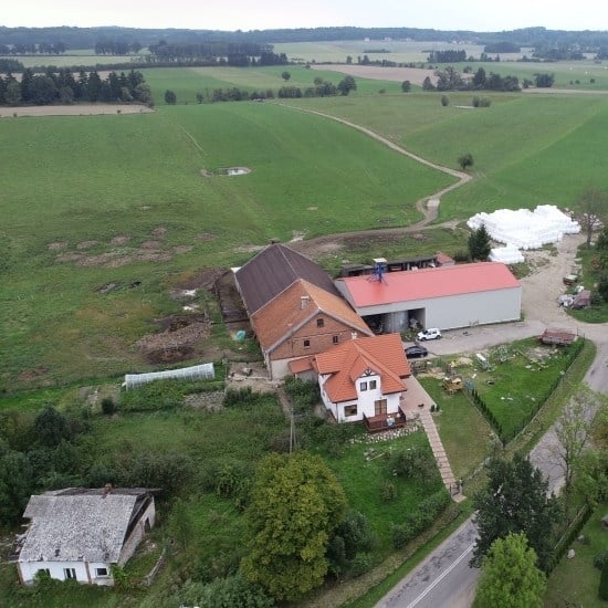
These discrepancies are clearly visible in land management practice and the resulting land-use structure [45]. Rural municipalities surrounding large cities are characterized by chaotic patterns of suburban development as well as fragmentation of agricultural land and forests whose initial functions are lost due to the irreversible depletion of their natural value (Figure 1).
Analyses of urban sprawl contribute to the discussion about the actual location of city boundaries which, due to administrative complexities and social resentment, are rarely changed. The term “urban sprawl” can be used to describe both a state (the degree of sprawl in a landscape) as well as a process (increasing sprawl in a landscape) [46]. The boundaries of cities can be identified by analyzing changes in the land cover of the affected space.
Urban sprawl can considerably influence the quality of life in various regions of the world. For this reason, urbanization trends and their extent should be closely monitored. Urban sprawl is often measured based on the population density gradient which marks the decrease in population density with an increase in distance from the urban core [47]. The size of the urban area is yet another measure of uncontrolled urbanization [48]. Analyses of population density and area support observations of the disproportional increase in urbanized space relative to the size of the urban population [49]. However, such analyses are complex and they often produce erroneous results. The increase in the number of users of rapidly expanding urban space is difficult to determine because these users formally reside in rural municipalities that surround the urban core.
A 1974 report entitled “The Costs of Sprawl” is one of the key documents illustrating the extent of urban sprawl and the methods for measuring this phenomenon [50]. The report proposes a sprawl index which is based on five measurable indicators: development density, land-use mix, structure of enterprises, activity centering in selected parts of the city, and road accessibility. The correlations between means of transport and socioeconomic potential were analyzed to reveal that people who live further away from the urban core are more likely to travel long distances, own more cars, and are even at greater risk of fatal traffic accidents [51].
3. Methods and Materials
3.1. Procedure
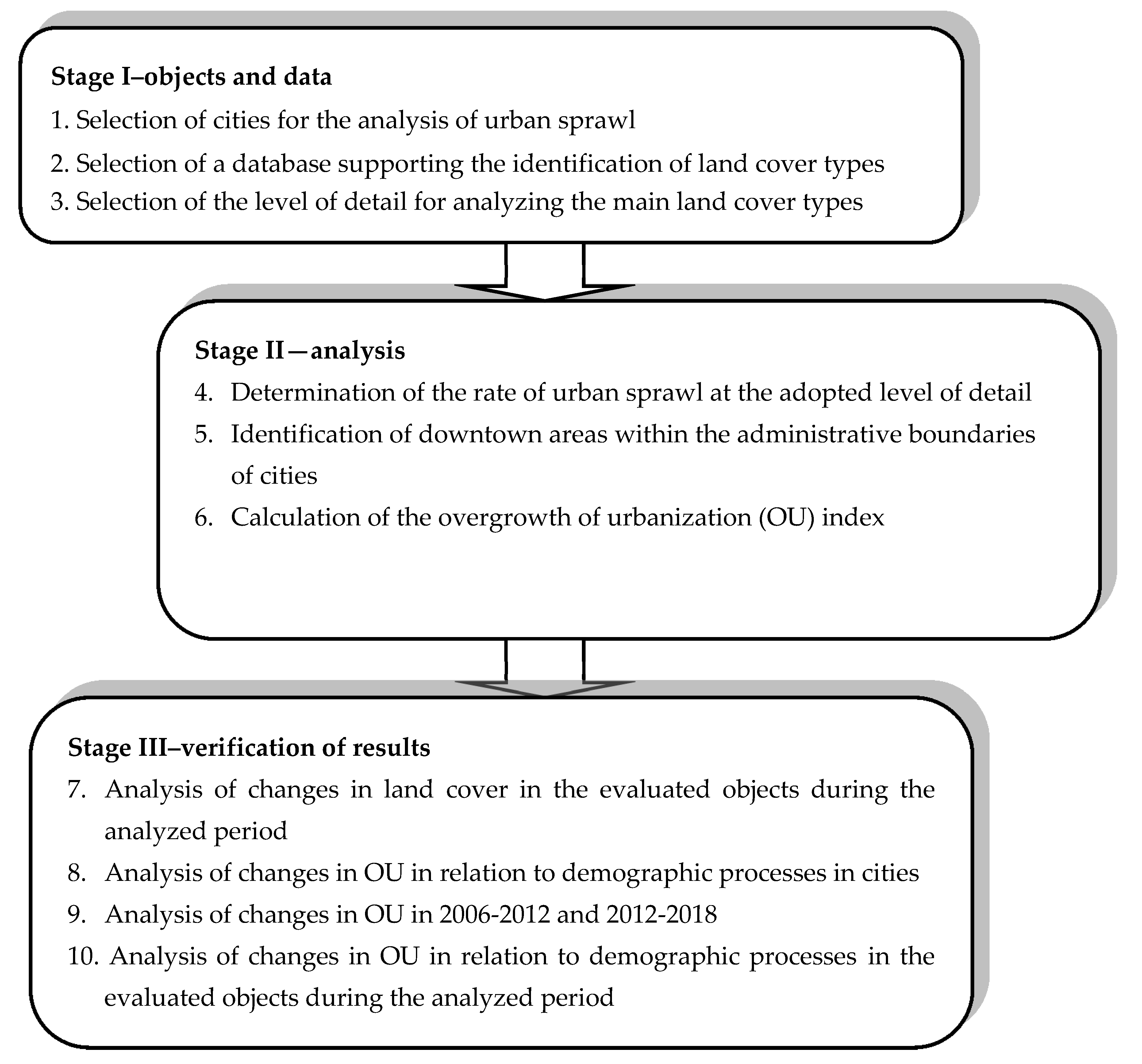
Due to complex data acquisition methods, research into urban sprawl is conducted in selected urban units and conducted over long periods of time. In studies of the type, data collection and analysis are time-consuming processes. In an attempt to develop new tools for monitoring uncontrolled urban sprawl on the national scale, this study proposes a procedure for calculating the overgrowth of urbanization (OU) index (Figure 2).
Cities that contribute to the overgrowth of urbanization were identified in the first stage of the analytical process. These cities can be selected based on various criteria, such as administrative status, economic significance, demographic data, or independent land-use planning systems. The latter criterion played the key role in this study. The selected cities are county capitals responsible for developing land-use plans that cover their respective territories and do not influence the adjacent areas. The boundaries of towns in the direct vicinity of the urban core were also aggregated in this stage of the analysis.
A database containing the required information on land cover was selected in the second stage of research. The selected database should ensure the spatial continuity and cyclicity of data. The CLC database fulfils the above requirements.
The required level of detail of land cover data was selected in the third stage. CLC data are available at three levels of detail. The selected level has to correspond to the research objective as well as the scale of the analysis. Highly detailed data could be required in studies that focus on individual cities to determine the extent and directions of urban sprawl. The present study investigated the degree of urbanization on the national scale; therefore, level 1 data were regarded as sufficient for the needs of the analysis.
The boundaries of the areas that have undergone urbanization were determined in the fourth stage. In this process, all level 1 areas, i.e., artificial surfaces, were aggregated. The actual boundaries of urbanized areas were determined based on their size and relative proximity. The current study analyzed the rate of urbanization; therefore, data covering different periods of time were required.
Level 1 areas within the administrative boundaries of the urban core were identified in the fifth stage.
The OU index was calculated in the sixth stage. The index was calculated as the ratio of an aggregated urban area to a city’s administrative area with the use of Equation (1):
where:
OU: overgrowth of urbanization index of area i;
Aga: aggregated urban area;
Ada: city’s administrative area;
i: number of analyzed areas.
The value of the OU index can range from zero to several or even more than ten points. The OU index can equal zero only in theory, as it would represent a situation where city boundaries have been mapped, but an urbanized area does not yet exist. When the OU index is higher than 0, but not higher than 1, the entire urbanized space is situated within the city’s administrative boundaries, and it is actually smaller than the area delimited by the city’s administrative boundaries. The above scenario is usually encountered in urban areas where extensive forests, surface water bodies, or agricultural land are situated within a city’s administrative boundaries. OU values higher than one indicates that urbanized space extends beyond a city’s boundaries.
Analyses of changes in land cover offer the simplest and the most rapid approach to measuring urbanized areas [55]. Land cover data are increasingly available from spatial databases and they can be rapidly processed with the use of GIS tools. These resources make analyses of urban sprawl less time consuming and they support analyses of a large number of cities, thus creating new sources of information for evaluating the extent and character of the evaluated phenomenon [56]. In this study, data for analysis were obtained from the CORINE Land Cover database. The analyzed data were generated by remote sensing. CLC data were processed by integrating remote sensing data in a mixed approach combining automatic methods and interpretation tools for digital image analysis. The processed data were Landsat TM multispectral satellite images and aerial images [57].
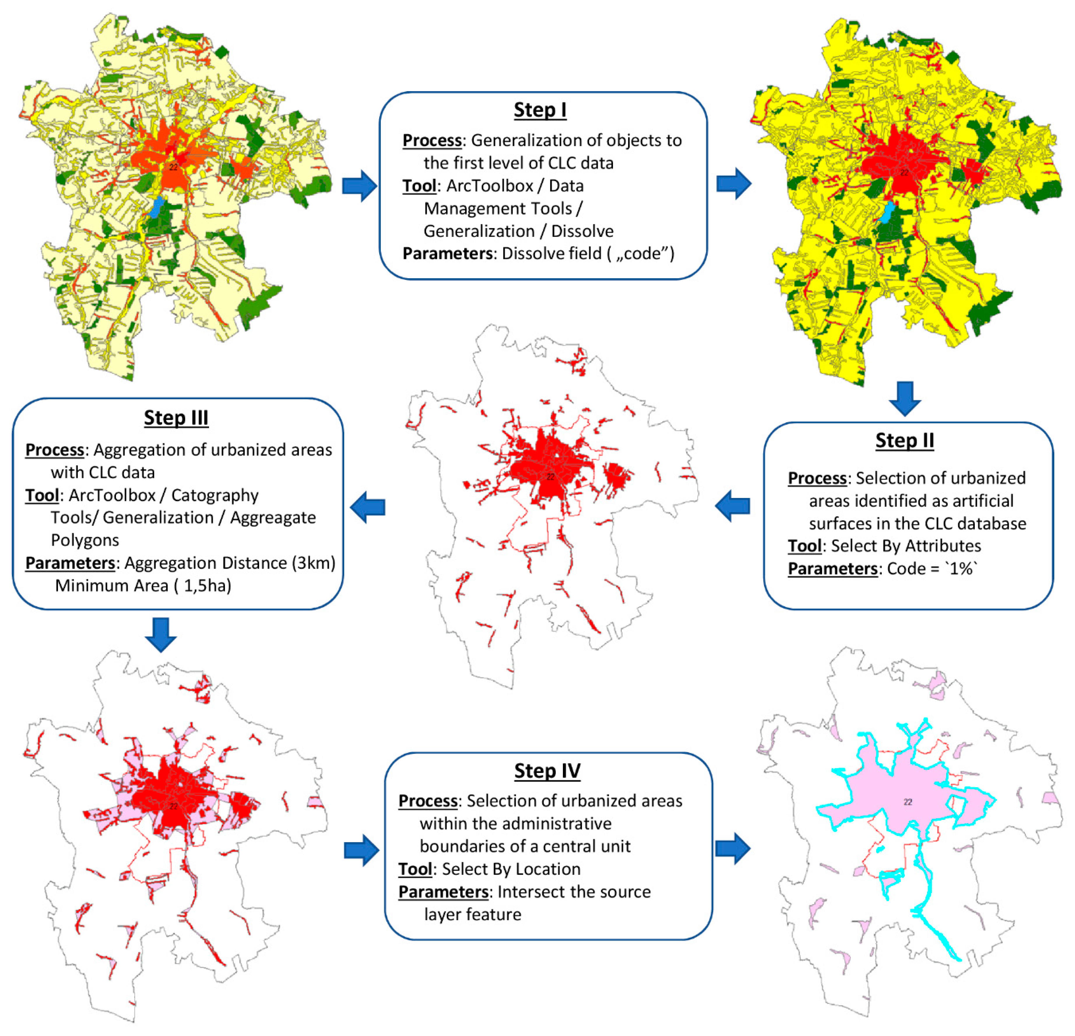
The procedure during which GIS tools were applied to determine the measures for calculating the OU index based on CLC data is presented in Figure 3.
The results of the calculations were verified in the third stage by analyzing changes in the value of OU. In the seventh stage, changes in land cover were determined based on CLC data for 2006, 2012, and 2018. In the eighth stage, changes in OU values were analyzed in relation to the demographic processes in the studied cities. The dynamics of urban sprawl was examined in the ninth stage by analyzing changes in OU values in 2006–2012 and 2012–2018. In the 10th stage, the rate of changes in OU values relative to demographic processes was determined in the evaluated objects during the analyzed period.
3.2. Data
The CORINE (Coordination of Information on the Environment) Land Cover program is a European Community initiative that was implemented in 1985. Poland joined the program in 2001 upon the decision of the Chief Inspector of Environmental Protection. The main aims of the CLC program are to [58]:
- compile harmonized information on the state of the environment with regard to certain topics which have priority for all Member States of the Community:
- coordinate the compilation of data and the organization of information within the Member States or at the international level;
- ensure that information is consistent and that data are compatible.
In Poland, the CLC project was carried out in 1990–2018 by the Institute of Geodesy and Cartography with financial support of the European Union. The results of the CLC project are presented on the website of the Chief Inspectorate of Environmental Protection.
The CLC database features all types of land cover on the European continent, and there are no headings for unclassified land [59]. The database contains information about land cover as well as land-use. Land cover nomenclature is organized at three levels. There are five main classes of land cover:
- Artificial surfaces—built-up areas, including residential areas, commercial and industrial areas, mines, and green urban spaces.
- Agricultural areas—arable land, permanent crops, meadows, pastures, and land principally occupied by agriculture with significant areas of natural vegetation.
- Forests and semi-natural areas—forests, shrubs and open areas with little or no vegetation.
- Wetlands—inland marshes, peatbogs, salt marshes, salines, and intertidal flats.
- Water bodies—inland waters and marine waters.
Different land-use types within each of the above groups are specified at the second and third level of the inventory [60].
The rate of urban sprawl in the analyzed cities was evaluated in areas classified as artificial surfaces in the CLC inventory (level 1). These areas were then aggregated based on their proximity and size. Urbanized areas separated by a distance of less than 3 km usually feature green urban areas and surface water bodies. This distance can be traveled without mechanized means of transport and can be crossed on foot, which contributes to social cohesion. As a result, the boundaries between such areas, if they formally exist, are weakly embedded in space and public awareness. Areas larger than 1.5 ha were also aggregated to eliminate isolated buildings such as forest service buildings, utility structures and technical facilities. The aggregation of urbanized areas larger than 1.5 ha supported the agglomeration of built-up land featuring at least several buildings and land that is permanently occupied or managed. In the next step, only areas where the central unit was situated within a city’s administrative area were selected. This procedure was conducted based on land cover data for 2006, 2012, and 2018.
The analysis covered cities, also referred to as central units, which are hubs of social and economic activity and create numerous opportunities for development. These areas implement independent spatial planning policies, which can deepen the divide between cities and the surrounding administrative units. The study involved Polish cities with the status of county capitals. These cities differ in levels of spatial, demographic, and economic development, and these parameters were included in the analysis of urban sprawl. A total of 71 Polish cities were evaluated. Two urban areas were merged to form agglomerations because the boundaries of the respective cities came into direct contact or were separated by a very small distance, thus forming a homogeneous urban structure. The merged areas were the Upper Silesian urban area composed of 19 cities and the Tricity urban area composed of five cities. In the final step, 49 urban areas with distinct administrative boundaries were identified. The studied area was determined in the land cover map by analyzing the increase in urbanization in the municipalities situated in the direct vicinity and at a small distance from the investigated city. Municipalities where the increase in urbanization proceeded in the direction of the urban core were included in the study. A total of 530 such municipalities were identified. The number or urban-rural municipalities and rural municipalities in the vicinity of the studied urban areas is presented in Table A1-Appendix A.
The size of urban areas and the surrounding municipalities, as well as information about changes in the administrative boundaries of cities in the last 20 years are also presented in Table A1. Administrative boundaries were changed in only six cities, and a significant increase in the size of urban areas was noted in only three cities: Zielona Góra (377%), Rzeszów (77%), and Opole (54%).
The analyzed areas, including the boundaries of 49 cities and the surrounding municipalities, are presented on a map of Polish voivodships in Figure 4.
4. Results
Land cover types in the analyzed areas were identified in the first stage of the study with the use of the CLC database. The corresponding data were divided into five main land cover classes corresponding to level 1 nomenclature in the CLC inventory. The analyzed data were not further subdivided into detailed land cover categories to prevent excessive fragmentation of the evaluated areas. The incorporation of more detailed data would prolong the analytical process without affecting the final result which is based on the size of all urbanized areas regardless of detailed land-use types. The land cover map of the analyzed areas based on level 1 nomenclature in the CLC database is presented in Figure 5. Land cover types in the examined areas were identified based on CLC data for three periods: CLC 2006, CLC 2012, and CLC 2018. This approach supported an evaluation of the rate of urbanization processes in the studied areas.
In the next step, the urban areas identified based on CLC 2006 data and classified as artificial surfaces were selected. Selected areas were aggregated based on their proximity and size. Only areas separated by a distance of up to 3 km were aggregated. The above criterion was applied to merge interdependent areas with a shared social and spatial structure. The analyzed areas were also merged based on their size. Only urban areas with a minimum size of 1.5 ha were aggregated. Distance and size criteria were adopted to identify and aggregate areas where non-isolated residential estates with direct spatial links to the urban core are being developed. Isolated residential enclaves were eliminated based on the literature. Some authors [61] define residential estates as clusters of minimum 10 residential buildings. Based on the average size of land plots zoned for residential construction (approx. 1200 m2) and the area required for the development of public facilities, the size criterion was set at 1.5 ha. The distance criterion was set based on the results of research investigating municipal transport and pedestrian zones. It was assumed that spatial differences between a city and the surrounding areas are obliterated if the place of residence and the nearest cluster of buildings are separated by walking distance. According to some authors, a walking distance of up to 5 km does not require extreme effort [62]. An analysis of the municipal transport system revealed that stops should not be separated by a distance greater than 2 km [63]. In view of the above, the distance criterion was set at up to 3 km. Several simulation tests were also carried out to modify the applied criteria. The adopted values produced optimal results and demonstrated a considerable shift in the boundaries of the urban zone.
Areas featuring individual buildings or temporary structures were thus eliminated from analysis. Areas that overlapped cities were identified, and urban areas that were directly linked to cities were identified in the last step. The above procedure was repeated for 2012 and 2018 data. The urban areas aggregated based on 2018, 2012, and 2006 data are presented in Figure 6. A clear increase in urbanization can be observed in the analyzed cities.
In the next step, the overgrowth of urbanization (OU) index was calculated as the ratio of aggregated urban area, determined in the previous step (Formula (1)), to the city’s administrative area. The values of the OU index in 2006, 2012, and 2018 with the corresponding size of urbanized areas are presented in Table A2.
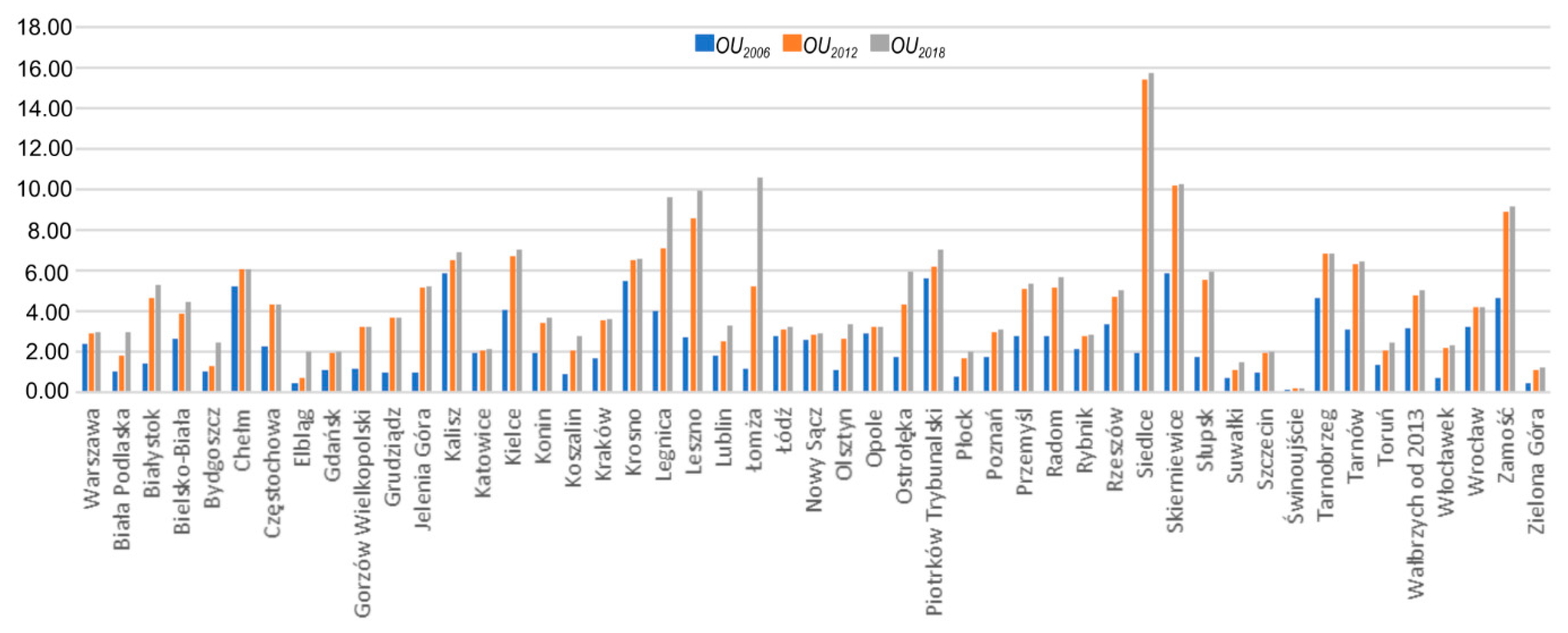
In the analyzed cities, the OU index in 2006, 2012, and 2018 was determined in the following range of values:
in 2006–from 0.17 in Świnoujście to 5.91 in Kalisz;
in 2012–from 0.22 w Świnoujście to 15.43 in Siedlce;
in 2018–from 0.23 w Świnoujście to 15.76 in Siedlce–Figure 7.
5. Discussion
The calculated values of the OU index support a comprehensive analysis of changes in cities and their immediate vicinity. In the first step of the analysis, the values of the OU index in 2006, 2012, and 2018 were compared based on demographic data. The cities identified as central units were divided into demographic classes based on their population. Central units with a population higher than 150,000 were classified as large cities; central units with a population of 80,000 to 150,000 were classified as medium-sized cities, and central units with a population below 80,000, as small cities. Small-, medium-, and large-sized cities are ranked in Table A3 with the corresponding values of the OU index.
The changes in the value of the OU index in each demographic class in 2006, 2012, and 2018 are presented in Figure 8. The OU index was highest in small cities in all analyzed years. The median value of OU clearly increased in small cities from 2.74 in 2006, to 6.10 in 2012, and 6.58 in 2018. Considerable variations in OU values were noted in small cities in the analyzed period. The third quartile of OU values was determined at 5.25 in 2006, 8.61 in 2012, and 9.97 in 2018, with an increasing number of outliers and the maximum OU value of 15.76. Such a dynamic increase in OU value was not observed in large and medium-sized cities. In large cities, the median value of OU reached 1.88 in 2006, 3.07 in 2012, and 3.33 in 2018. In medium-sized cities, this parameter was determined at 3.07, 3.22, and 3.25, respectively. Large- and medium-sized cities were also characterized by smaller variations in OU values. In large cities, the values between the first and the third quartile ranged from 1.30 to 2.79 in 2006, from 2.08 to 4.40 in 2012, and from 2.47 to 4.60 in 2018. A somewhat greater range of values was observed in medium-sized cities: from 0.84 to 3.07 in 2006, from 2.13 to 5.49 in 2012, and from 2.44 to 5.76 in 2018. The number of outliers increased in both groups.
In the step, the values of the OU index were analyzed over time. In 2006–2012, the highest increase in urbanized area was noted in Siedlce (698.80%) and the smallest increase was observed in Katowice (6.70%). In 2012–2018, the corresponding increase was highest in Elbląg (179.03%) and lowest in Wrocław (0.06%). The analyzed cities are ranked based on the values of the OU index in 2006–2012 in Figure 9 and in 2012–2018 in Figure 10.
The increase in OU values was also investigated in demographic classes to analyze the results of the performed calculations. In large cities with a population higher than 150,000, urbanization processes were most extensive in 2006–2012 in Białystok (227.17%) and least extensive in Katowice (6.70%). In 2012–2018, urbanization proceeded most rapidly in Bydgoszcz (90.65%) and least rapidly in Wrocław (0.06%). In medium-sized cities with a population of 80,000 to 150,000, urbanization was highest in 2006–2012 in Jelenia Góra (419.50%) and lowest in Nowy Sącz (10.14%). In 2012–2018, the increase in urbanization was highest in Elbąg (179.03%) and lowest in Grudziądz (0.12%). In small cities with a population below 80,000, urbanization proceeded most rapidly in 2006–2012 in Siedlce (698.80%) and least rapidly in Piotrków Trybunalski (10.60%). In 2012–2018, the increase in urbanization was highest in Łomża (101.91%) and lowest in Chełm (0.22%). The cities in each demographic class are ranked based on the increase in the values of the OU index in Table A4.
In the next step, the changes in the value of the OU index were referenced with population changes in the analyzed objects. The increase in OU values in 2006–2012 and 2012–2018 with an increase in the population of the analyzed cities and the adjacent municipalities are presented in Table A5.
The distribution of the increase in the analyzed values is presented graphically in Figure 11. The smallest changes in population were observed in small cities where the median value of OU reached 0.05 and the values between the first and third quartile ranged from 0.05 to 0.36. Much greater changes in population with more diversified median values were noted in large cities in 2006–2012, where the increase in the OU indicator was smallest relative to the remaining demographic classes. The values of OU were also clustered near the median value (0.65) and the values between the first and the third quartile ranged from 0.54 to 3.42. The smallest increase in population (median: 0.48) with a large number of outliers (range of values between the first and third quartile: −0.80 to 1.35) was observed in medium-sized cities which were characterized by the highest increase in OU values (median: 1.08) and similar change trends (range of values between the first and the third quartile: 0.35 to 1.99, without outliers). In small cities, the increase in OU was higher (median: 0.76; range of values between the first and the third quartile: 0.33 to 1.48, without outliers) and more stable than the increase in population (median: 0.77; range of values between the first and the third quartile: 0.025 to 1.26, with a large number of outliers).
An analysis of the increase in OU values and population in 2012–2018 produced somewhat different results. These changes are presented graphically in Figure 12. The increase in OU values in all demographic classes was close to zero, and significant variations were not observed. The greatest variations in OU values were noted in small cities, where the median reached 0.05 and the range of values between the first and the third quartile was determined at 0.05 to 0.36. The population increase in 2012–2018 was much greater and more diversified relevant to the median. The observed trends were similar to those observed in the previous period. The greatest differences were noted in large cities, where the median reached 0.98 and the range of values between the first and the third quartile was determined at −0.49 to 2.73. Population increased at a much slower rate in small cities, where the median reached −0.54 and the range of values between the first and the third quartile was determined at −1.54 to 0.19. The smallest, but the most varied increase was observed in medium-sized cities where the median reached −0.38 and the range of values between the first and the third quartile was determined at −1.36 to 0.40, with a large number of outliers.
6. Conclusions
Urban sprawl is one of the most important determinants of the present and future structure of cities and areas that directly undergo urbanization. The extent and rate of urban sprawl can be evaluated by analyzing spatial data relating to different land cover types.
The results of the present study indicate that the CLC database is a reliable source of information about urbanization processes. Several conclusions can be drawn from the analysis of the OU index in areas surrounding the capital cities of Polish counties. The analysis demonstrated that the CLC database is highly useful for evaluating urban sprawl phenomena in all evaluated cities. The OU index is a simple and effective tool for analyzing the extent of urban sprawl. An analysis of changes in OU values over time also produced valuable findings. The CLC inventory is regularly updated, which supports reliable evaluations of the dynamics of spatial phenomena such as urban sprawl. An analysis of OU values over time revealed two distinctive periods of spatial changes: a more dynamic period in 2006–2012 and a more stable period in 2012–2018. A clear increase in urbanized area in the vicinity of the analyzed cities was noted in 2006–2012 and it coincided with a boom on the Polish real estate market. The above period witnessed a rapid increase in built-up area (residential and road construction) in the vicinity of most cities. Urbanization processes were considerably slowed down in 2012–2018.
The examined cities were divided into three demographic classes based on their population and an analysis conducted in each class also produced interesting results. Large cities were characterized by a smaller increase in urbanized area than medium- and small-sized cities. These findings could be attributed to already high levels of urbanization in the analyzed areas and a reduction in the distance that could be comfortably traveled by residents who commute to work in the urban core. These results could pave the way to future research into development density in urbanized areas. The above findings could also indicate that the studied cities are less affected by urban sprawl. Different results were noted in areas neighboring small cities which were characterized by very high values of the OU index. However, considerable variations in OU values were noted in this group, which suggests that small cities “spill” over much larger areas. The above could also result from much greater availability of undeveloped land and the annexation of smaller towns in the vicinity of cities due to the expansion of the road network and improved transport accessibility.
The results noted in different demographic classes were also confronted with an analysis of population changes in the examined cities. Despite a smaller increase in urbanized area, large cities witnessed a substantial increase in population. These findings validate the observation that urbanized areas are characterized by high development density, but further research is needed to confirm this hypothesis. The smallest increase in population or, in some cases, a population decrease was observed in small cities. Therefore, it could be postulated that in small cities, urbanization does not increase with a rise in demand, but that it increases in response to an improvement in the quality of life and greater availability of undeveloped land. Small cities were characterized by considerable variations in the value of the OU index which were not associated with a population increase, which suggests that urban sprawl is a much more rapid and unpredictable process in this group.
Despite a relatively small increase in the population of medium-sized cities, the distribution of the OU index was relatively stable both in terms of its values and growth dynamics.
A uniform land cover database is very difficult to develop for large areas. The growing number of Earth observation satellites supports the creation of cohesive land cover databases. Satellite images are regularly available for all regions of the Earth (provided that cloud cover is low), and they can be collected with high frequency at a relatively low cost. Satellite data have to be processed in a rigorous and systematic manner and in relation to the existing data to maximize the reliability of the resulting databases. The above requirements have to be met to ensure that the collected data are consistent and that they produce uniform sets of land cover data. The CORINE Land Cover (CLC) inventory is a prime example of the above [64]. The latest CLC inventories are generated based on satellite images that are interpreted with the use of semi-automatic, computer-aided methods which reduce processing time. In addition to SPOT−4/5 data (2006), CLC databases also rely on optical imaging systems that acquire satellite images in the near-infrared spectrum, such as Landsat-7’s ETM (2000), IRS P6’s sensor LISS III (2006 and 2012) and RapidEye (2012) [65].
The extent to which the acquired data can be used in the CLC inventory is limited mainly by their scope and level of detail. The CLC inventory is an excellent source of data for small-scale studies, but its applicability for large-scale analyses is controversial. One of the limitations could be the minimum polygon area which was set at 25 ha for a polygon with a minimum width of 100 m. In areas characterized by various types of land cover, the polygon represents the predominant land-use type. The use of the dominant land cover in highly fragmented landscapes can lead to considerable generalization. For this reason, clear and stable criteria have to be applied to produce reliable results in studies where changes in land cover are analyzed over time. These criteria are an integral element of the CLC inventory and they play an important role in the present study.
The results of this study indicate that the CLC database is particularly useful for analyzing the rate of changes in land cover and the accompanying spatial phenomena such as urban sprawl. The relevant data can be analyzed to produce far-reaching conclusions about the dynamics and magnitude of urbanization processes. Subsequent updates of the CLC inventory will expand the range of data for analyses and even more interesting conclusions could be derived if the CLC database were updated more frequently.
This study analyzed urbanization processes in areas surrounding the capital cities of Polish counties across time and in different demographic classes; therefore, the research goal has been achieved. The presented findings can be used in further research to expand the thematic and spatial scope of similar analyses.
Author Contributions
Conceptualization, I.C.; Data curation, A.B., I.C.; Formal analysis, A.B.; Methodology, I.C.; Project administration, A.B., S.C.; Supervision, I.C.; Visualization, K.S.; Writing—original draft, A.B., I.C.; Writing—review & editing, A.B. All authors have read and agreed to the published version of the manuscript.
Funding
This research received no external funding.
Acknowledgments
The Corine Land Cover project in Poland was implemented by the Institute of Geodesy and Cartography and financed by the European Union. Project results were obtained from the website of the Chief Inspectorate for Environmental Protection clc.gios.gov.pl.
Conflicts of Interest
The authors declare no conflict of interest.
Appendix A

Table A1.
The studied urban areas and the surrounding municipalities.
| No. | Urban Area | Area [ha] in 2018 | Year of Change in Administrat-ive Boundaries | Change in Area [%] | Area [ha] of Adjacent Municipalities | Number of Adminis-trative Units |
|---|---|---|---|---|---|---|
| 1 | Warszawa | 51,724 | 189,299 | 26 | ||
| 2 | Biała Podlaska | 4940 | 104,058 | 6 | ||
| 3 | Białystok | 10,213 | 139,414 | 8 | ||
| 4 | Bielsko-Biała | 12,451 | 84,710 | 15 | ||
| 5 | Bydgoszcz | 17,598 | 174,801 | 10 | ||
| 6 | Chełm | 3528 | 95,501 | 7 | ||
| 7 | Częstochowa | 15,971 | 105,456 | 10 | ||
| 8 | Elbląg | 7982 | 98,764 | 7 | ||
| 9 | Tricity urban area | 46,431 | 166,127 | 15 | ||
| 10 | Gorzów Wielkopolski | 8572 | 97,513 | 6 | ||
| 11 | Grudziądz | 5776 | 107,937 | 9 | ||
| 12 | Jelenia Góra | 10,922 | 112,979 | 13 | ||
| 13 | Kalisz | 6942 | 97,475 | 8 | ||
| 14 | Upper Silesian urban area | 141,440 | 403,177 | 57 | ||
| 15 | Kielce | 10,965 | 119,897 | 11 | ||
| 16 | Konin | 8220 | 97,177 | 9 | ||
| 17 | Koszalin | 9834 | 2010 | 18.0 | 99,089 | 7 |
| 18 | Kraków | 32,685 | 142,849 | 17 | ||
| 19 | Krosno | 4350 | 70,726 | 10 | ||
| 20 | Legnica | 5629 | 97,083 | 8 | ||
| 21 | Leszno | 3186 | 80,100 | 6 | ||
| 22 | Lublin | 14,747 | 109,372 | 11 | ||
| 23 | Łomża | 3267 | 116,209 | 7 | ||
| 24 | Łódź | 29,325 | 158,095 | 16 | ||
| 25 | Nowy Sącz | 5758 | 64,206 | 8 | ||
| 26 | Olsztyn | 8833 | 145,151 | 7 | ||
| 27 | Opole | 14,888 | 2017 | 54.2 | 95,761 | 9 |
| 28 | Ostrołęka | 2863 | 71,378 | 5 | ||
| 29 | Piotrków Trybunalski | 6724 | 98,007 | 7 | ||
| 30 | Płock | 8804 | 116,051 | 9 | ||
| 31 | Poznań | 1351 | 136,318 | 12 | ||
| 32 | Przemyśl | 26,191 | 2010 | 5.5 | 66,544 | 7 |
| 33 | Radom | 4617 | 122,064 | 11 | ||
| 34 | Rybnik | 11,180 | 168,026 | 27 | ||
| 35 | Rzeszów | 14,836 | 2006–2017 | 76.9 | 116,904 | 13 |
| 36 | Siedlce | 12,041 | 99,932 | 8 | ||
| 37 | Skierniewice | 3186 | 2012 | 4.6 | 75,450 | 8 |
| 38 | Słupsk | 3460 | 123,343 | 6 | ||
| 39 | Suwałki | 4315 | 96,424 | 6 | ||
| 40 | Szczecin | 6551 | 173,931 | 8 | ||
| 41 | Świnoujście | 30,060 | 113,008 | 5 | ||
| 42 | Tarnobrzeg | 19,723 | 96,115 | 10 | ||
| 43 | Tarnów | 8540 | 77,071 | 9 | ||
| 44 | Toruń | 7238 | 98,921 | 7 | ||
| 45 | Wałbrzych | 11,572 | 98,377 | 13 | ||
| 46 | Włocławek | 8470 | 106,018 | 9 | ||
| 47 | Wrocław | 29,282 | 171,653 | 11 | ||
| 48 | Zamość | 3034 | 52,303 | 5 | ||
| 49 | Zielona Góra | 27,832 | 2015 | 377.1 | 177,313 | 11 |
| Total | 5,828,077 | 530 |
Table A2.
Overgrowth of urbanization index in 2006, 2012 and 2018. The calculated indicators OU for 2006, 2012 and 2018 are marked in gray.
Table A2.
Overgrowth of urbanization index in 2006, 2012 and 2018. The calculated indicators OU for 2006, 2012 and 2018 are marked in gray.
| No. | Urban Area | Urbanized Area 2006 (ha) | Urbanized Area 2012 (ha) | Urbanized Area 2018 (ha) | OU 2006 | OU 2012 | OU 2018 |
|---|---|---|---|---|---|---|---|
| 1 | Warszawa | 123,502 | 152,496 | 154,533 | 2.39 | 2.95 | 2.99 |
| 2 | Biała Podlaska | 5102 | 9107 | 14,878 | 1.03 | 1.84 | 3.01 |
| 3 | Białystok | 14,466 | 47,328 | 54,276 | 1.42 | 4.63 | 5.31 |
| 4 | Bielsko-Biała | 32,928 | 48,442 | 55,340 | 2.65 | 3.90 | 4.45 |
| 5 | Bydgoszcz | 18,778 | 22,500 | 42,895 | 1.07 | 1.28 | 2.44 |
| 6 | Chełm | 18,531 | 21,547 | 21,593 | 5.25 | 6.10 | 6.11 |
| 7 | Częstochowa | 36,543 | 68,872 | 69,578 | 2.29 | 4.32 | 4.36 |
| 8 | Elbląg | 3801 | 5751 | 16,047 | 0.48 | 0.72 | 2.01 |
| 9 | Gdańsk | 47,394 | 81,448 | 83,255 | 1.15 | 1.97 | 2.01 |
| 10 | Gorzów Wielkopolski | 9897 | 27,582 | 27,915 | 1.15 | 3.22 | 3.26 |
| 11 | Grudziądz | 5612 | 21,408 | 21,433 | 0.97 | 3.71 | 3.72 |
| 12 | Jelenia Góra | 10,933 | 56,798 | 57,453 | 1.00 | 5.20 | 5.26 |
| 13 | Kalisz | 40,951 | 45,476 | 47,767 | 5.91 | 6.56 | 6.89 |
| 14 | Katowice | 237,193 | 253,096 | 260,582 | 1.95 | 2.08 | 2.14 |
| 15 | Kielce | 44,589 | 73,438 | 77,506 | 4.07 | 6.70 | 7.08 |
| 16 | Konin | 16,058 | 28,283 | 30,242 | 1.96 | 3.45 | 3.69 |
| 17 | Koszalin | 9220 | 20,560 | 27,615 | 0.94 | 2.09 | 2.81 |
| 18 | Kraków | 54,517 | 116,685 | 118,896 | 1.67 | 3.57 | 3.64 |
| 19 | Krosno | 23,996 | 28,517 | 28,593 | 5.52 | 6.56 | 6.58 |
| 20 | Legnica | 22,671 | 40,088 | 54,220 | 4.03 | 7.12 | 9.64 |
| 21 | Leszno | 8711 | 27,414 | 31,752 | 2.74 | 8.61 | 9.97 |
| 22 | Lublin | 26,690 | 37,303 | 48,431 | 1.81 | 2.53 | 3.28 |
| 23 | Łomża | 3780 | 17,141 | 34,609 | 1.16 | 5.25 | 10.60 |
| 24 | Łódź | 81,830 | 91,901 | 94,813 | 2.79 | 3.14 | 3.24 |
| 25 | Nowy Sącz | 14,920 | 16,433 | 16,843 | 2.59 | 2.86 | 2.93 |
| 26 | Olsztyn | 9866 | 23,399 | 29,737 | 1.12 | 2.65 | 3.37 |
| 27 | Opole | 43,309 | 48,084 | 48,323 | 2.91 | 3.23 | 3.25 |
| 28 | Ostrołęka | 5885 | 14,596 | 19,912 | 1.76 | 4.37 | 5.96 |
| 29 | Piotrków Trybunalski | 37,823 | 41,831 | 47,414 | 5.63 | 6.23 | 7.06 |
| 30 | Płock | 7110 | 15,057 | 17,925 | 0.81 | 1.71 | 2.04 |
| 31 | Poznań | 46,385 | 78,733 | 82,310 | 1.77 | 3.01 | 3.15 |
| 32 | Przemyśl | 12,986 | 23,521 | 24,701 | 2.81 | 5.09 | 5.35 |
| 33 | Radom | 31,078 | 57,736 | 63,385 | 2.78 | 5.17 | 5.67 |
| 34 | Rybnik | 64,712 | 83,894 | 84,590 | 2.17 | 2.82 | 2.84 |
| 35 | Rzeszów | 40,380 | 57,280 | 60,669 | 3.35 | 4.76 | 5.04 |
| 36 | Siedlce | 6152 | 49,139 | 50,212 | 1.93 | 15.43 | 15.76 |
| 37 | Skierniewice | 20,380 | 35,322 | 35,527 | 5.90 | 10.22 | 10.28 |
| 38 | Słupsk | 7615 | 24,114 | 25,535 | 1.77 | 5.59 | 5.92 |
| 39 | Suwałki | 4667 | 7123 | 10,005 | 0.71 | 1.09 | 1.53 |
| 40 | Szczecin | 29,904 | 59,683 | 59,859 | 0.99 | 1.98 | 1.99 |
| 41 | Świnoujście | 3436 | 4570 | 4687 | 0.17 | 0.23 | 0.23 |
| 42 | Tarnobrzeg | 40,027 | 58,337 | 58,523 | 4.69 | 6.83 | 6.86 |
| 43 | Tarnów | 22,556 | 46,015 | 46,770 | 3.12 | 6.36 | 6.47 |
| 44 | Toruń | 15,657 | 24,025 | 28,690 | 1.35 | 2.08 | 2.48 |
| 45 | Wałbrzych | 26,800 | 40,587 | 42,716 | 3.17 | 4.80 | 5.05 |
| 46 | Włocławek | 6118 | 18,731 | 19,479 | 0.73 | 2.22 | 2.31 |
| 47 | Wrocław | 94,562 | 122,463 | 122,538 | 3.23 | 4.19 | 4.19 |
| 48 | Zamość | 14,228 | 27,098 | 27,955 | 4.69 | 8.93 | 9.21 |
| 49 | Zielona Góra | 13,937 | 30,187 | 34,731 | 0.50 | 1.08 | 1.25 |
Table A3.
Ranking of cities based on population with the corresponding values of the OU index. Demographic classes of cities have been marked in color. Big cities—blue, medium—orange, small—green.
Table A3.
Ranking of cities based on population with the corresponding values of the OU index. Demographic classes of cities have been marked in color. Big cities—blue, medium—orange, small—green.
| No. | Urban Area | OU Index 2006 | OU Index 2012 | OU Index 2018 | Population in 2017 |
|---|---|---|---|---|---|
| 1 | Warszawa | 2.39 | 2.95 | 2.99 | 1,764,615 |
| 18 | Kraków | 1.67 | 3.57 | 3.64 | 767,348 |
| 24 | Łódź | 2.79 | 3.14 | 3.24 | 690,422 |
| 47 | Wrocław | 3.23 | 4.19 | 4.19 | 638,586 |
| 31 | Poznań | 1.77 | 3.01 | 3.15 | 538,633 |
| 9 | Gdańsk | 1.15 | 1.97 | 2.01 | 464,254 |
| 40 | Szczecin | 0.99 | 1.98 | 1.99 | 403,883 |
| 5 | Bydgoszcz | 1.07 | 1.28 | 2.44 | 352,313 |
| 22 | Lublin | 1.81 | 2.53 | 3.28 | 339,850 |
| 3 | Białystok | 1.42 | 4.63 | 5.31 | 297,288 |
| 14 | Katowice | 1.95 | 2.08 | 2.14 | 296,262 |
| 7 | Częstochowa | 2.29 | 4.32 | 4.36 | 224,376 |
| 33 | Radom | 2.78 | 5.17 | 5.67 | 214,566 |
| 44 | Toruń | 1.35 | 2.08 | 2.48 | 202,562 |
| 15 | Kielce | 4.07 | 6.70 | 7.08 | 196,804 |
| 35 | Rzeszów | 3.35 | 4.76 | 5.04 | 189,662 |
| 26 | Olsztyn | 1.12 | 2.65 | 3.37 | 173,070 |
| 4 | Bielsko-Biała | 2.65 | 3.90 | 4.45 | 171,505 |
| 49 | Zielona Góra | 0.50 | 1.08 | 1.25 | 139,819 |
| 34 | Rybnik | 2.17 | 2.82 | 2.84 | 139,129 |
| 27 | Opole | 2.91 | 3.23 | 3.25 | 128,140 |
| 10 | Gorzów Wielkopolski | 1.15 | 3.22 | 3.26 | 124,295 |
| 8 | Elbląg | 0.48 | 0.72 | 2.01 | 120,895 |
| 30 | Płock | 0.81 | 1.71 | 2.04 | 120,787 |
| 45 | Wałbrzych since 2013 | 3.17 | 4.80 | 5.05 | 113,621 |
| 46 | Włocławek | 0.73 | 2.22 | 2.31 | 111,752 |
| 43 | Tarnów | 3.12 | 6.36 | 6.47 | 109,650 |
| 17 | Koszalin | 0.94 | 2.09 | 2.81 | 107,670 |
| 13 | Kalisz | 5.91 | 6.56 | 6.89 | 101,625 |
| 20 | Legnica | 4.03 | 7.12 | 9.64 | 100,324 |
| 11 | Grudziądz | 0.97 | 3.71 | 3.72 | 95,629 |
| 38 | Słupsk | 1.77 | 5.59 | 5.92 | 91,465 |
| 25 | Nowy Sącz | 2.59 | 2.86 | 2.93 | 84,041 |
| 12 | Jelenia Góra | 1.00 | 5.20 | 5.26 | 80,072 |
| 36 | Siedlce | 1.93 | 15.43 | 15.76 | 77,653 |
| 16 | Konin | 1.96 | 3.45 | 3.69 | 74,834 |
| 29 | Piotrków Trybunalski | 5.63 | 6.23 | 7.06 | 74,312 |
| 39 | Suwałki | 0.71 | 1.09 | 1.53 | 69,554 |
| 48 | Zamość | 4.69 | 8.93 | 9.21 | 64,354 |
| 21 | Leszno | 2.74 | 8.61 | 9.97 | 64,197 |
| 6 | Chełm | 5.25 | 6.10 | 6.11 | 63,333 |
| 23 | Łomża | 1.16 | 5.25 | 10.60 | 63,092 |
| 32 | Przemyśl | 2.81 | 5.09 | 5.35 | 61,808 |
| 2 | Biała Podlaska | 1.03 | 1.84 | 3.01 | 57,545 |
| 28 | Ostrołęka | 1.76 | 4.37 | 5.96 | 52,215 |
| 37 | Skierniewice | 5.90 | 10.22 | 10.28 | 48,308 |
| 42 | Tarnobrzeg | 4.69 | 6.83 | 6.86 | 47,387 |
| 19 | Krosno | 5.52 | 6.56 | 6.58 | 46,600 |
| 41 | Świnoujście | 0.17 | 0.23 | 0.23 | 41,032 |
Table A4.
Ranking of cities based on an increase in the values of the OU index in 2006–2012 and 2012–2018 and an increase in population. Demographic classes of cities have been marked in color. Big cities—blue, medium—orange, small—green.
Table A4.
Ranking of cities based on an increase in the values of the OU index in 2006–2012 and 2012–2018 and an increase in population. Demographic classes of cities have been marked in color. Big cities—blue, medium—orange, small—green.
| No. | Urban Area | Population in 2017 | Increase in OU in 2006–2012 (%) | No. | Urban Area | Population in 2017 | Increase in OU in 2012–2018 (%) |
|---|---|---|---|---|---|---|---|
| 3 | Białystok | 297,288 | 227.17 | 5 | Bydgoszcz | 352,313 | 90.65 |
| 26 | Olsztyn | 173,070 | 137.16 | 22 | Lublin | 339,850 | 29.83 |
| 18 | Kraków | 767,348 | 114.04 | 26 | Olsztyn | 173,070 | 27.09 |
| 40 | Szczecin | 403,883 | 99.58 | 44 | Toruń | 202,562 | 19.42 |
| 7 | Częstochowa | 224,376 | 88.47 | 3 | Białystok | 297,288 | 14.68 |
| 33 | Radom | 214,566 | 85.78 | 4 | Bielsko-Biała | 171,505 | 14.24 |
| 9 | Gdańsk | 464,254 | 71.85 | 33 | Radom | 214,566 | 9.78 |
| 31 | Poznań | 538,633 | 69.74 | 35 | Rzeszów | 189,662 | 5.92 |
| 15 | Kielce | 196,804 | 64.70 | 15 | Kielce | 196,804 | 5.54 |
| 44 | Toruń | 202,562 | 53.45 | 31 | Poznań | 538,633 | 4.54 |
| 4 | Bielsko-Biała | 171,505 | 47.11 | 24 | Łódź | 690,422 | 3.17 |
| 35 | Rzeszów | 189,662 | 41.85 | 14 | Katowice | 296,262 | 2.96 |
| 22 | Lublin | 339,850 | 39.76 | 9 | Gdańsk | 464,254 | 2.22 |
| 47 | Wrocław | 638,586 | 29.51 | 18 | Kraków | 767,348 | 1.89 |
| 1 | Warszawa | 1,764,615 | 23.48 | 1 | Warszawa | 1764,615 | 1.34 |
| 5 | Bydgoszcz | 352,313 | 19.82 | 7 | Częstochowa | 224,376 | 1.02 |
| 24 | Łódź | 690,422 | 12.31 | 40 | Szczecin | 403,883 | 0.29 |
| 14 | Katowice | 296,262 | 6.70 | 47 | Wrocław | 638,586 | 0.06 |
| 12 | Jelenia Góra | 80,072 | 419.50 | 8 | Elbląg | 120,895 | 179.03 |
| 11 | Grudziądz | 95,629 | 281.49 | 20 | Legnica | 100,324 | 35.25 |
| 38 | Słupsk | 91,465 | 216.65 | 17 | Koszalin | 107,670 | 34.32 |
| 46 | Włocławek | 111,752 | 206.18 | 30 | Płock | 120,787 | 19.05 |
| 10 | Gorzów Wielkopolski | 124,295 | 178.68 | 49 | Zielona Góra | 139,819 | 15.05 |
| 17 | Koszalin | 107,670 | 122.99 | 38 | Słupsk | 91,465 | 5.89 |
| 49 | Zielona Góra | 139,819 | 116.60 | 45 | Wałbrzych | 113,621 | 5.25 |
| 30 | Płock | 120,787 | 111.77 | 13 | Kalisz | 101,625 | 5.04 |
| 43 | Tarnów | 109,650 | 104.00 | 46 | Włocławek | 111,752 | 3.99 |
| 20 | Legnica | 100,324 | 76.82 | 25 | Nowy Sącz | 84,041 | 2.49 |
| 45 | Wałbrzych | 113,621 | 51.44 | 43 | Tarnów | 109,650 | 1.64 |
| 8 | Elbląg | 120,895 | 51.28 | 10 | Gorzów Wielkopolski | 124,295 | 1.21 |
| 34 | Rybnik | 139,129 | 29.64 | 12 | Jelenia Góra | 80,072 | 1.15 |
| 13 | Kalisz | 101,625 | 11.05 | 34 | Rybnik | 139,129 | 0.83 |
| 27 | Opole | 128,140 | 11.03 | 27 | Opole | 128,140 | 0.50 |
| 25 | Nowy Sącz | 84,041 | 10.14 | 11 | Grudziądz | 95,629 | 0.12 |
| 36 | Siedlce | 77,653 | 698.80 | 23 | Łomża | 63,092 | 101.91 |
| 23 | Łomża | 63,092 | 353.39 | 2 | Biała Podlaska | 57,545 | 63.36 |
| 21 | Leszno | 64,197 | 214.70 | 39 | Suwałki | 69,554 | 40.47 |
| 28 | Ostrołęka | 52,215 | 148.03 | 28 | Ostrołęka | 52,215 | 36.42 |
| 48 | Zamość | 64,354 | 90.46 | 21 | Leszno | 64,197 | 15.83 |
| 32 | Przemyśl | 61,808 | 81.13 | 29 | Piotrków Trybunalski | 74,312 | 13.35 |
| 2 | Biała Podlaska | 57,545 | 78.51 | 16 | Konin | 74,834 | 6.92 |
| 16 | Konin | 74,834 | 76.13 | 32 | Przemyśl | 61,808 | 5.02 |
| 37 | Skierniewice | 48,308 | 73.32 | 48 | Zamość | 64,354 | 3.16 |
| 39 | Suwałki | 69,554 | 52.63 | 36 | Siedlce | 77,653 | 2.18 |
| 42 | Tarnobrzeg | 47,387 | 45.74 | 41 | Świnoujście | 41,032 | 2.12 |
| 41 | Świnoujście | 41,032 | 33.00 | 37 | Skierniewice | 48,308 | 0.58 |
| 19 | Krosno | 46,600 | 18.84 | 42 | Tarnobrzeg | 47,387 | 0.32 |
| 6 | Chełm | 63,333 | 16.28 | 19 | Krosno | 46,600 | 0.27 |
| 29 | Piotrków Trybunalski | 74,312 | 10.60 | 6 | Chełm | 63,333 | 0.22 |
Table A5.
Ranking of cities based on an increase in the values of the OU index and an increase in population. Demographic classes of cities have been marked in color. Big cities—blue, medium—orange, small—green.
Table A5.
Ranking of cities based on an increase in the values of the OU index and an increase in population. Demographic classes of cities have been marked in color. Big cities—blue, medium—orange, small—green.
| Name | Urban Area | Increase in OU 06-12 | Increase in OU 12-18 | Population Increase 06-12 | Population Increase 12-18 |
|---|---|---|---|---|---|
| 1 | Warszawa | 0.23 | 0.01 | 3.33 | 3.73 |
| 18 | Kraków | 1.14 | 0.02 | 2.78 | 2.54 |
| 24 | Łódź | 0.12 | 0.03 | −3.19 | −2.55 |
| 47 | Wrocław | 0.30 | 0.00 | 2.95 | 3.45 |
| 31 | Poznań | 0.70 | 0.05 | 3.75 | 2.81 |
| 9 | Gdańsk | 0.72 | 0.02 | 3.67 | 2.70 |
| 40 | Szczecin | 1.00 | 0.00 | 2.25 | 0.20 |
| 5 | Bydgoszcz | 0.20 | 0.91 | 2.45 | −0.29 |
| 22 | Lublin | 0.40 | 0.30 | 0.76 | −0.43 |
| 3 | Białystok | 2.27 | 0.15 | 2.15 | 1.92 |
| 14 | Katowice | 0.07 | 0.03 | −2.21 | −2.04 |
| 7 | Częstochowa | 0.88 | 0.01 | −2.01 | −2.67 |
| 33 | Radom | 0.86 | 0.10 | −0.15 | −0.67 |
| 44 | Toruń | 0.53 | 0.19 | 1.77 | 1.29 |
| 15 | Kielce | 0.65 | 0.06 | 5.05 | −0.12 |
| 35 | Rzeszów | 0.42 | 0.06 | 4.18 | 3.71 |
| 26 | Olsztyn | 1.37 | 0.27 | 3.02 | 1.25 |
| 4 | Bielsko-Biała | 0.47 | 0.14 | 1.96 | 0.71 |
| 49 | Zielona Góra | 1.17 | 0.15 | 1.30 | 8.34 |
| 34 | Rybnik | 0.30 | 0.01 | 0.68 | −0.22 |
| 27 | Opole | 0.11 | 0.00 | −2.69 | −1.03 |
| 10 | Gorzów Wielkopolski | 1.79 | 0.01 | 1.78 | 0.89 |
| 8 | Elbląg | 0.51 | 1.79 | −0.77 | −1.72 |
| 30 | Płock | 1.12 | 0.19 | 0.29 | −0.68 |
| 45 | Wałbrzych since 2013 | 0.51 | 0.05 | −1.72 | −3.42 |
| 46 | Włocławek | 2.06 | 0.04 | −0.82 | −2.13 |
| 43 | Tarnów | 1.04 | 0.02 | 0.05 | −0.40 |
| 17 | Koszalin | 1.23 | 0.34 | 2.34 | −0.19 |
| 13 | Kalisz | 0.11 | 0.05 | −0.67 | −0.91 |
| 20 | Legnica | 0.77 | 0.35 | 1.37 | 0.32 |
| 11 | Grudziądz | 2.81 | 0.00 | 0.83 | −0.91 |
| 38 | Słupsk | 2.17 | 0.06 | 1.05 | −0.29 |
| 25 | Nowy Sącz | 0.10 | 0.02 | 3.45 | 1.88 |
| 12 | Jelenia Góra | 4.19 | 0.01 | −1.40 | −2.50 |
| 36 | Siedlce | 6.99 | 0.02 | 0.97 | 1.43 |
| 16 | Konin | 0.76 | 0.07 | 0.92 | −0.57 |
| 29 | Piotrków Trybunalski | 0.11 | 0.13 | −0.82 | −1.36 |
| 39 | Suwałki | 0.53 | 0.40 | 1.26 | 0.40 |
| 48 | Zamość | 0.90 | 0.03 | 0.72 | −0.66 |
| 21 | Leszno | 2.15 | 0.16 | 2.86 | 0.80 |
| 6 | Chełm | 0.16 | 0.00 | −0.94 | −2.27 |
| 23 | Łomża | 3.53 | 1.02 | 0.77 | −0.19 |
| 32 | Przemyśl | 0.81 | 0.05 | −0.25 | −1.43 |
| 2 | Biała Podlaska | 0.79 | 0.63 | 0.65 | −0.39 |
| 28 | Ostrołęka | 1.48 | 0.36 | 2.01 | 0.82 |
| 37 | Skierniewice | 0.73 | 0.01 | 0.53 | −0.06 |
| 42 | Tarnobrzeg | 0.46 | 0.00 | −1.11 | −2.03 |
| 19 | Krosno | 0.19 | 0.00 | 1.10 | −0.14 |
| 41 | Świnoujście | 0.33 | 0.02 | 1.82 | −1.19 |
References
- Cieślak, I. Identification of areas exposed to land use conflict with the use of multiple-criteria decision-making methods. Land Use Policy 2019, 89, 104225. [Google Scholar] [CrossRef]
- Lisowski, A. Problems with the contemporary identification of the concept of ‘suburbanization’. In Urban Agglomerations in Poland at the Turn of the 20th and 21st Centuries: Problems of Development of Structural Transformations and Functioning; Maik, W., Ed.; Wydawnictwo Uczelniane WSG: Bydgoszcz, Poland, 2009; pp. 59–72. (In Polish) [Google Scholar]
- Glaeser, E.; Kahn, M.E. Sprawl and Urban Growth NBER Working Paper Series 2003. Working Paper 9733. Available online: http://www.nber.org/papers/w9733 (accessed on 1 November 2019).
- Crisci, M.; Gemmiti, R.; Proietti, E.; Violante, A. Urban Sprawl e Shrinking Cities in Italia. Trasformazione Urbana e Redistribuzione della Popolazione nelle Aree Metropolitan; CNR-IRPPS e-Publishing: Roma, Italy, 2014. [Google Scholar]
- EEA Report. Urban Sprawl in Europe—The Ignored Challenge; Report No 10/2006; European Environment Agency: Copenhagen, Denmark, 2006. Available online: http://www.eea.europa.eu/publications/eea_report_2006_10 (accessed on 12 November 2019).
- Zuziak, Z.K. Suburban area in the city’s architecture: Towards the new architecture of the urban region. In The Problem of Suburbanization; Lorens, P., Ed.; Biblioteka Urbanisty: Warsaw, Poland, 2005; pp. 17–32. (In Polish) [Google Scholar]
- Kociuba, D. Limitations in urban development in the context of spatial planning, (Ograniczenia w rozwoju miast w kontekście planowania przestrzennego). Studia KPZK PAN 2015, 161, 112–122. (In Polish) [Google Scholar]
- Śleszyński, P.; Deręgowska, A.; Kubiak, Ł.; Sudra, P.; Zielińska, B. Analysis of the State and Conditions of Planning Work in Municipalities in 2017; Instytut Geografii i Przestrzennego Zagospodarowania PAN na zlecenie Ministerstwa Inwestycji i Rozwoju: Warsaw, Poland, 2018. (In Polish) [Google Scholar]
- Cieślak, I.; Czyża, S.; Szuniewicz, K.; Ogrodniczak, M. Assessment of Residential Areas of City on the Example of Olsztyn. In IOP Conference Series: Materials Science and Engineering; IOP Publishing: Bristol, UK, 2019; Volume 471, p. 102001. [Google Scholar] [CrossRef]
- Borana, S.L.; Yadav, S.K. Urban Growth Analysis Using Shannon’s Entropy: A Case Study of Jodhpur City. Int. J. 2017, 5, 50–57. [Google Scholar]
- Hassea, J.; Lathrop, R. Land resource impact indicators of urban sprawl. Appl. Geogr. 2003, 23, 159–175. [Google Scholar] [CrossRef]
- Zagajewski, B.; Jarocińska, A.; Olesiuk, D. Methods and Techniques of Geoinformatic Research (Metody i Techniki Badań Geoinformatycznych); Wydział Geografii i Studiów Regionalnych UW: Warsaw, Poland, 2009; pp. 1–117. (In Polish) [Google Scholar]
- Pelorosso, R.; Leone, A.; Boccia, L. Land cover and land use change in the Italian central Apennines: A comparison of assessment methods. Appl. Geogr. 2009, 29, 35–48. [Google Scholar] [CrossRef]
- Cieślak, I.; Szuniewicz, K.; Czyża, S. Analysis of the Variation of the Areas under Urbanization Pressure Using Entropy Index. Procedia Eng. 2016, 161, 2001–2005. [Google Scholar] [CrossRef] [Green Version]
- Ustaoglu, E.; Aydınoglu, A.C. Regional Variations of Land-Use Development and Land-Use/Cover Change Dynamics: A Case Study of Turkey. Remote Sens. 2019, 11, 885. [Google Scholar] [CrossRef] [Green Version]
- Grigorescu, I.; Kucsicsa, G.; Popovici, E.; Mitrică, B.; Dumitrașcu, M.; Mocanu, I. Regional disparities in the urban sprawl phenomenon in Romania using CORINE land cover database. Rom. J. Geogr. 2018, 62, 169–184. [Google Scholar]
- Bathrellos, G.D.; Skilodimou, H.D.; Chousianitis, K.; Youssef, A.M.; Pradhan, B. Multi-hazard assessment modeling via multi-criteria analysis and GIS: A case study. Sci. Total Environ. 2017, 575, 119–134. [Google Scholar] [CrossRef]
- Jucha, W.; Kroczak, R. Comparison of land use data from the CORINE Land Cover program with data obtained from orthophotomaps. In Socio-Economic and Spatial Transformation of Regional Structures; Kaczmarska, E., Raźniak, P., Eds.; Oficyna Wydawnicza AFM: Kraków, Poland, 2014; pp. 123–136. (In Polish) [Google Scholar]
- Bruegmann, R. Sprawl: A Compact History; University of Chicago Press: Chicago, IL, USA; London, UK, 2005. [Google Scholar]
- Degórska, B. Spatial Urbanization of Rural Areas in the Warsaw Metropolitan Area. Ecological and Landscape Context; Instytut Geografii I Przestrzennego Zagospodarowania PAN: Warsaw, Poland, 2017. (In Polish) [Google Scholar]
- Lewyn, M. Sprawl in Europe and America. San Diego Law Rev. 2009, 46, 85. [Google Scholar] [CrossRef] [Green Version]
- EEA Report. Urban Sprawl in Europe, Joint EEA-FOEN Report; EEA Report No. 11/2016; European Environment Agency—Publications Office of the European Union: Luxembourg, 2016; Available online: https://www.eea.europa.eu/publications/urban-sprawl-in-europe (accessed on 10 November 2019).
- Kudłacz, M. Dysfunctions of amorphous settlement growth in Poland. Studia Ekonomiczne 2016, 279, 245–257. (In Polish) [Google Scholar]
- Leontidou, L.; Afouxenidis, A.; Kourliouros, E.; Marmaras, E. Infrastructure related urban sprawl: Mega-events and hybrid peri-urban landscapes in Southern Europe. In Urban Sprawl in Europe: Landscape, Land-Use Change and Policy; Couch, C., Leontidou, L., Petschel-Held, G., Eds.; Blackwell Publishing: Hoboken, NJ, USA, 2007; pp. 71–101. [Google Scholar]
- Jaeger, J.A.G.; Schwick, C. Improving the measurement of urban sprawl: Weighted Urban Proliferation (WUP) and Its application to Switzerland. Ecol. Indic. 2014, 38, 294–308. [Google Scholar] [CrossRef]
- Zhao, P. Managing urban growth in a transforming China: Evidence from Beijing. Land Use Policy 2011, 28, 96–109. [Google Scholar] [CrossRef]
- Batho, S.; Williams, G.; Russell, L. Responding to urban crisis: The emergency planning response to the bombing of Manchester city centre. Cities 2000, 17, 293–304. [Google Scholar] [CrossRef]
- Parry, I.W.; Walls, M.; Harrington, W. Automobile externalities and policies. J. Econ. Lit. 2007, 45, 373–399. [Google Scholar] [CrossRef]
- Batty, M.; Besussi, E.; Chin, N. Traffic, Urban Growth and Suburban Sprawl; Centre for Advanced Spatial Analysis University College: London, UK, 2003. [Google Scholar]
- Litwińska, E. Modeling of metropolitan structures in the aspect of the phenomenon of urban sprawl. Czasopismo Techniczne Architektura 2010, 107, 139–148. (In Polish) [Google Scholar]
- Nechyba, T.J.; Walsh, R.P. Urban sprawl. J. Econ. Perspect. 2004, 18, 177–200. [Google Scholar] [CrossRef] [Green Version]
- Cieślak, I.; Szuniewicz, K.; Gerus-Gościewska, M. Evaluation of the Natural Value of Land Before and after Planning Procedures. Rural Dev. 2013, 6, 3. [Google Scholar]
- Nelson, A.C.; Sanchez, T.W. The effectiveness of urban containment regimes in reducing exurban sprawl. Plan. Rev. 2005, 41, 42–47. [Google Scholar] [CrossRef]
- Cieślak, I. Spatial conflicts: Analyzing a burden created by differing land use. Acta Geogr. Slov. 2019, 59. [Google Scholar] [CrossRef] [Green Version]
- Galster, G.; Hanson, R.; Ratcliffe, M.R.; Wolman, H.; Coleman, S.; Freihage, J. Wrestling sprawl to the ground: Defining and measuring an elusive concept. Hous. Policy Debate 2001, 12, 681–717. [Google Scholar] [CrossRef]
- Ewing, R. Is Los Angeles-style sprawl desirable? J. Am. Plan. Assoc. 1997, 63, 107–126. [Google Scholar] [CrossRef]
- Bilozor, A.; Renigier-Bilozor, M. Procedure of Assessing Usefulness of the Land in the Process of Optimal Investment Location for Multi-Family Housing Function. Procedia Eng. 2016, 161, 1868–1873. [Google Scholar] [CrossRef] [Green Version]
- Biłozor, A.; Renigier-Biłozor, M.; Cellmer, R. Assessment Procedure of Suburban Land Attractiveness and Usability for Housing. In Proceedings of the 2018 Baltic Geodetic Congress, Olsztyn, Poland, 21–23 June 2018. [Google Scholar] [CrossRef]
- Renigier-Bilozor, M.; Bilozor, A. Optimization of the Variables Selection in the Process of Real Estate Markets Rating. Oeconomia Copernicana 2015, 6, 139–157. [Google Scholar] [CrossRef]
- Ready, R.; Abdalla, C. GIS Analysis of Land Use on the Rural-Urban Fringe: The Impact of Land Use and Potential Local Disamenities on Residential Property Values and on the Location of Residential Development in Berks County; 2007 Final Report. Staff Paper 364 June 2003; The Northeast Regional Center for Rural Development: Philadelphia, PA, USA, 2003. [Google Scholar]
- Renigier-Bilozor, M.; Wisniewski, R.; Bilozor, A. Rating attributes toolkit for the residential property market. Int. J. Strateg. Prop. Mnang. 2017, 21, 307–317. [Google Scholar] [CrossRef]
- Renigier-Bilozor, M. Modern classification system of real estate markets. Geod. Vestn. 2017, 61, 441–460. [Google Scholar] [CrossRef]
- Wojtkun, G. Are cities really growing? Czasopismo Techniczne Architektura 2010, 107, 311–317. (In Polish) [Google Scholar]
- Zachariasz, I. Legal conditions for the effectiveness of plans. Zarządzanie Publiczne 2013, 23, 5–16. (In Polish) [Google Scholar]
- Ghosh, S. A city growth and land-use/land-cover change: A case study of Bhopal, India. Model. Earth Syst. Environ. 2019, 5, 1569–1578. [Google Scholar] [CrossRef]
- Jaeger, J.A.G.; Bertiller, R.; Schwick, C.; Kienast, F. Suitability criteria for measures of urban sprawl. Ecol. Indic. 2010, 10, 397–406. [Google Scholar] [CrossRef]
- Mils, E. Studiesin fhe Structureofthe Urban Economy; Johns Hopkins Press: Baltimore, MD, USA, 1972. [Google Scholar]
- O’sullivan, A. Urban Economics; McGraw-Hill/Irwin: New York, NY, USA, 2007; pp. 225–226. [Google Scholar]
- Geshkov, M. Urban sprawl in Eastern Europe: The Sofia City example. Econ. Altern. 2015, 2, 101–116. [Google Scholar]
- Real Estate Research Corporation, Council on Environmental Quality (US), United States; Department of Housing, Urban Development; Office of Policy Development, & United States; Environmental Protection Agency; Office of Planning. The Costs of Sprawl: Environmental and Economic Costs of Alternative Residential Development Patterns at the Urban Fringe; The Council on Environmental Quality, the Office of Policy Development and Research, Department of Housing and Urban Development, and the Office of Planning and Management, Environmental Protection Agency US Government Printing Office: Portland, OR, USA, 1974; Volume 1.
- Lisowski, A. Urban sprawl process. In Urban Sprawl: Warsaw Agglomeration Case Study; Gutry-Korycka, M., Ed.; Warsaw University Press: Warsaw, Poland, 2005; pp. 83–99. [Google Scholar]
- Bhalli, M.N.; Ghaffar, A.; Shirazi, S.A. Remote Sensing and GIS applications for monitoring and assessment of the urban sprawl in Faisalabad-Pakistan. Pak. J. Sci. 2012, 64, 203–208. [Google Scholar]
- Skilodimou, H.D.; Bathrellos, G.D.; Chousianitis, K.; Youssef, A.M.; Pradhan, B. Multi-hazard assessment modeling via multi-criteria analysis and GIS: A case study. Environ. Earth Sci. 2019, 78, 47. [Google Scholar] [CrossRef]
- Biłozor, A.; Czyża, S.; Bajerowski, T. Identification and Location of a Transitional Zone between an Urban and a Rural Area Using Fuzzy Set Theory, CLC, and HRL Data. Sustainability 2019, 11, 7014. [Google Scholar] [CrossRef] [Green Version]
- Bielecka, E.; Jenerowicz, A. Intellectual Structure of CORINE Land Cover Research Applications in Web of Science: A Europe-Wide Review. Remote Sens. 2019, 11, 2017. [Google Scholar] [CrossRef] [Green Version]
- Cieślak, I.; Szuniewicz, K.; Pawlewicz, K.; Czyża, S. Land Use Changes Monitoring with CORINE Land Cover Data. In IOP Conference Series: Materials Science and Engineering; IOP Publishing: Bristol, UK, 2017; Volume 245, p. 052049. [Google Scholar] [CrossRef] [Green Version]
- Stathopoulou, M.; Cartalis, C.; Petrakis, M. Integrating Corine Land Cover data and Landsat TM for surface emissivity definition: Application to the urban area of Athens, Greece. Int. J. Remote Sens. 2017, 28, 3291–3304. [Google Scholar] [CrossRef]
- Chief Inspectorate of Environmental Protection. CORINE Land Cover (CLC) Programme. Available online: https://clc.gios.gov.pl/ (accessed on 1 May 2017). (In Poland)
- Petrişor, A.I. Using CORINE data to look at deforestation in Romania: Distribution & possible consequences. Urbanism. Arhitectură 2015, 6, 83–90. [Google Scholar]
- Bielecka, E.; Ciołkosz, A. Poland CLC-2006. Polski Przegląd Kartograficzny 2009, 41, 227–236. (In Polish) [Google Scholar]
- Podawca, K.; Górecki, M. Analysis of housing conditions in selected closed suburbs near Warsaw. Urban Dev. Probl. 2009, 1, 94–107. (In Polish) [Google Scholar]
- Böhm, A. Spatial Planning for Landscape Architects; Politechnika Krakowska: Kraków, Poland, 2006. (In Polish) [Google Scholar]
- Local Government Portal. Public Transport in Provincial Cities. Where the Furthest to the Stop. Available online: https://www.portalsamorzadowy.pl/gospodarka-komunalna/transport-publiczny-w-miastach-wojewodzkich-gdzie-najdalej-do-przystanku,103786.html (accessed on 4 December 2019). (In Polish).
- Leinenkugel, P.; Deck, R.; Huth, J.; Ottinger, M.; Mack, B. The potential of open geodata for automated large-scale land use and land cover classification. Remote Sens. 2019, 11, 2249. [Google Scholar] [CrossRef] [Green Version]
- Büttner, G.; Maucha, G. The Thematic Accuracy of Corine Land Cover 2000. Assessment Using LUCAS (Land Use/Cover Area Frame Statistical Survey); European Environment Agency: Copenhagen, Denmark, 2006; Volume 7. Available online: www.eea.europa.eu (accessed on 1 November 2019).
Figure 1.
Progressive development in the suburban zone–southern part of the Olsztyn city in the Region of Warmia and Mazury, Poland. Source: own elaboration.
Figure 1.
Progressive development in the suburban zone–southern part of the Olsztyn city in the Region of Warmia and Mazury, Poland. Source: own elaboration.

Figure 2.
Procedure of calculating the overgrowth of urbanization (OU) index and verifying the results.
Figure 2.
Procedure of calculating the overgrowth of urbanization (OU) index and verifying the results.

Figure 3.
The application of Geographic Information System (GIS) tools for spatial analysis.

Figure 4.
Source: own elaboration.

Figure 5.
Land cover map of the analyzed areas based on CLC data (level 1). Source: own elaboration.
Figure 5.
Land cover map of the analyzed areas based on CLC data (level 1). Source: own elaboration.

Figure 6.
Aggregated urban areas. Source: own elaboration.

Figure 7.
The OU index in the analyzed cities. Source: own elaboration.

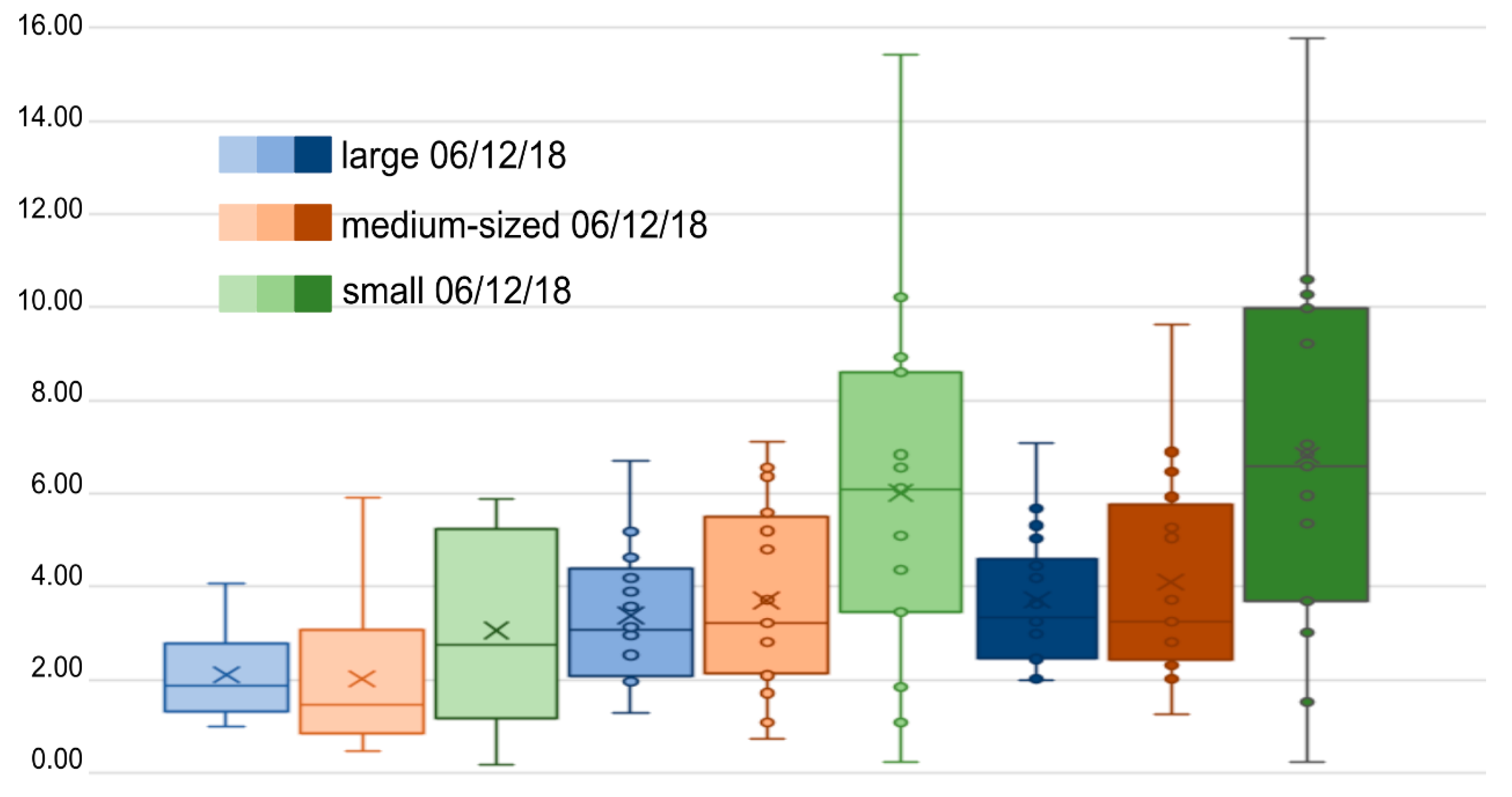
Figure 8.
The value of the OU index in demographic classes in 2006, 2012, and 2018.

Figure 9.
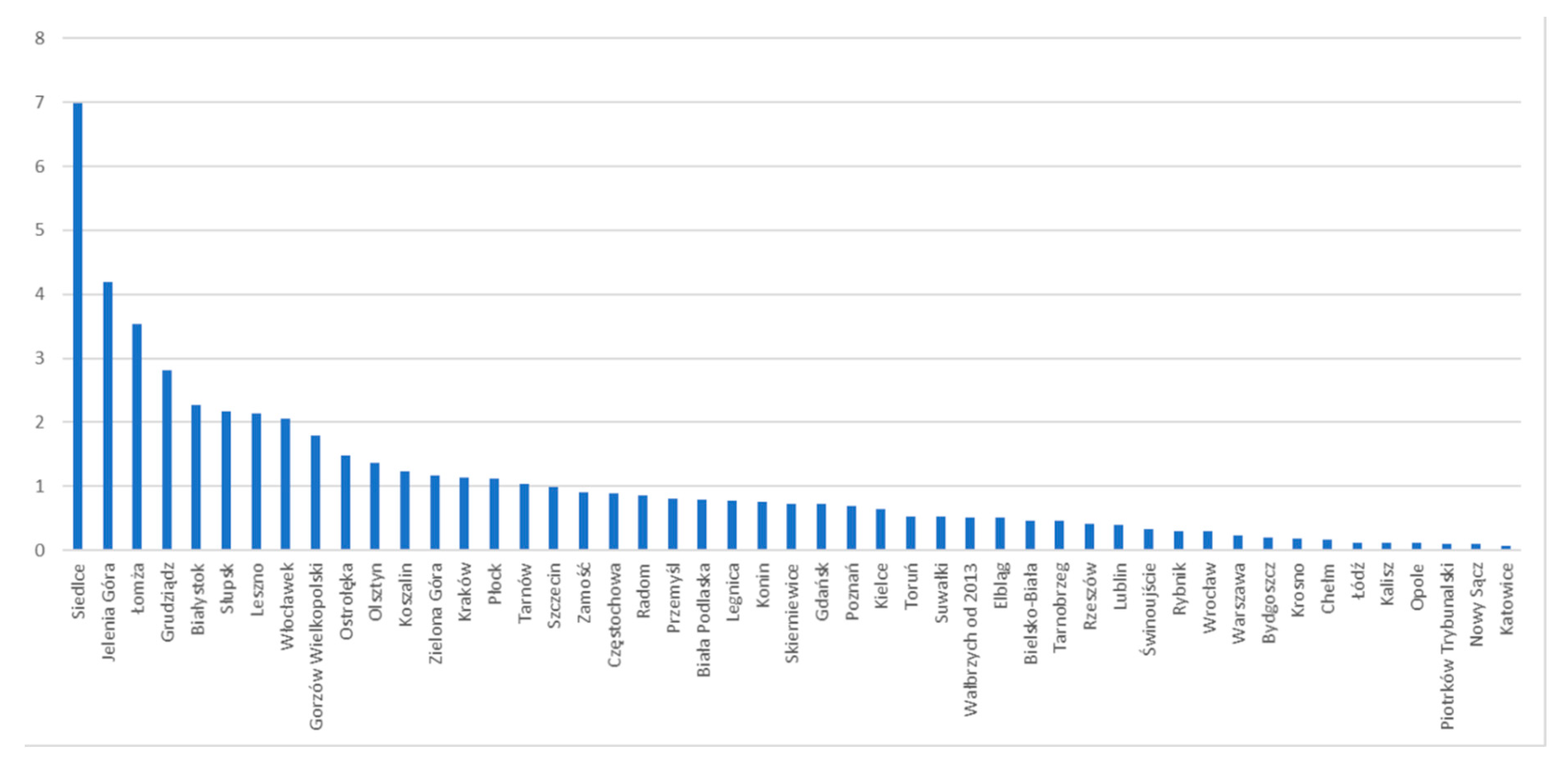
Ranking of cites based on the values of the OU index in 2006–2012.

Figure 10.
Ranking of cites based on the values of the OU index in 2012–2018.

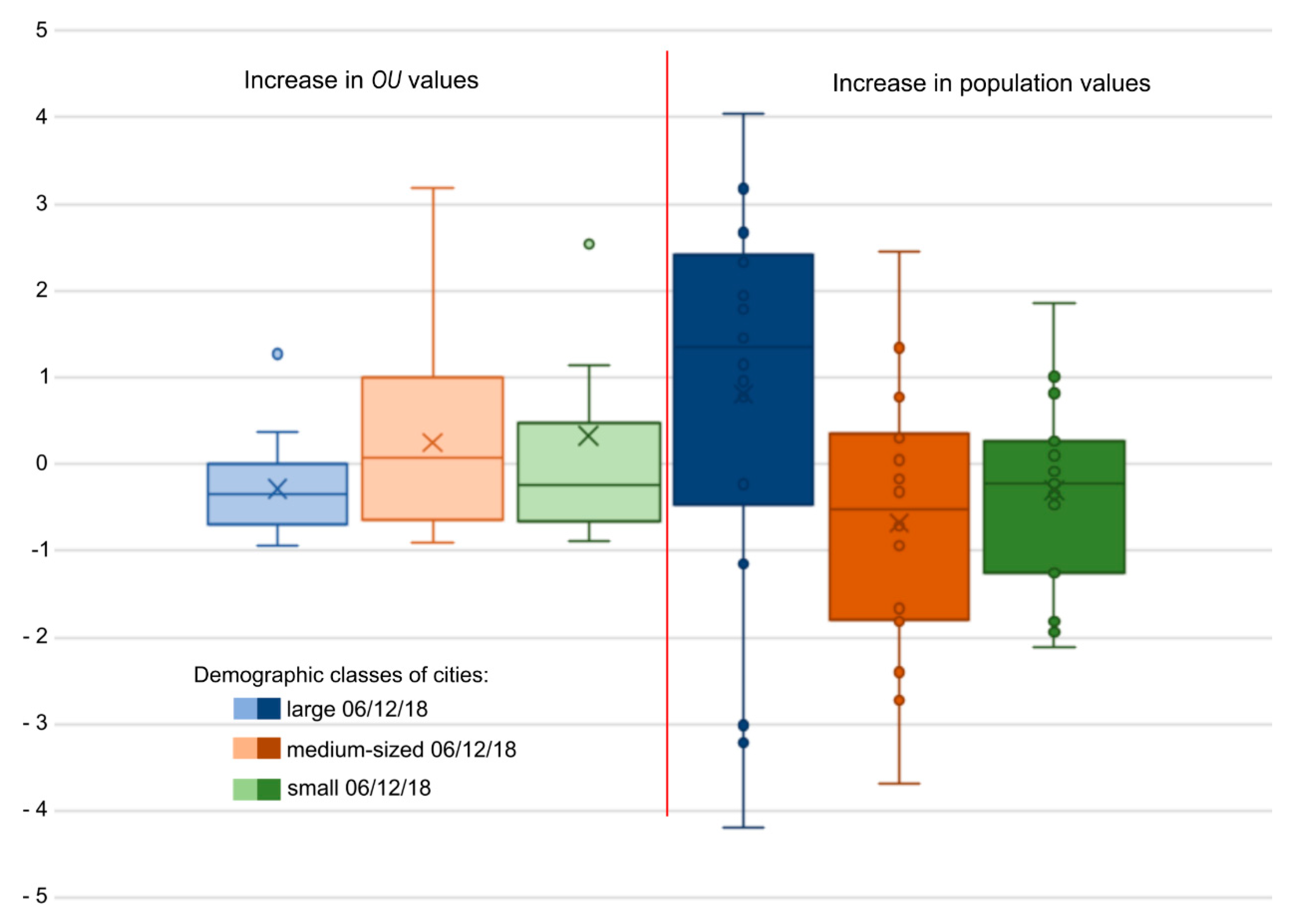
Figure 11.
Increase in OU values and population in 2006–2012.

Figure 12.
Increase in OU values and population in 2012–2018.

© 2020 by the authors. Licensee MDPI, Basel, Switzerland. This article is an open access article distributed under the terms and conditions of the Creative Commons Attribution (CC BY) license (http://creativecommons.org/licenses/by/4.0/).
Share and Cite
MDPI and ACS Style
Cieślak, I.; Biłozor, A.; Szuniewicz, K. The Use of the CORINE Land Cover (CLC) Database for Analyzing Urban Sprawl. Remote Sens. 2020, 12, 282. https://doi.org/10.3390/rs12020282
AMA Style
Cieślak I, Biłozor A, Szuniewicz K. The Use of the CORINE Land Cover (CLC) Database for Analyzing Urban Sprawl. Remote Sensing. 2020; 12(2):282. https://doi.org/10.3390/rs12020282
Chicago/Turabian StyleCieślak, Iwona, Andrzej Biłozor, and Karol Szuniewicz. 2020. "The Use of the CORINE Land Cover (CLC) Database for Analyzing Urban Sprawl" Remote Sensing 12, no. 2: 282. https://doi.org/10.3390/rs12020282
Note that from the first issue of 2016, this journal uses article numbers instead of page numbers. See further details here.