Abstract
Proper satellite-based crop monitoring applications at the farm-level often require near-daily imagery at medium to high spatial resolution. The combination of data from different ongoing satellite missions Sentinel 2 (ESA) and Landsat 7/8 (NASA) provides this unprecedented opportunity at a global scale; however, this is rarely implemented because these procedures are data demanding and computationally intensive. This study developed a robust stream processing for the harmonization of Landsat 7, Landsat 8 and Sentinel 2 in the Google Earth Engine cloud platform, connecting the benefit of coherent data structure, built-in functions and computational power in the Google Cloud. The harmonized surface reflectance images were generated for two agricultural schemes in Bekaa (Lebanon) and Ninh Thuan (Vietnam) during 2018–2019. We evaluated the performance of several pre-processing steps needed for the harmonization including the image co-registration, Bidirectional Reflectance Distribution Functions correction, topographic correction, and band adjustment. We found that the misregistration between Landsat 8 and Sentinel 2 images varied from 10 m in Ninh Thuan (Vietnam) to 32 m in Bekaa (Lebanon), and posed a great impact on the quality of the final harmonized data set if not treated. Analysis of a pair of overlapped L8-S2 images over the Bekaa region showed that, after the harmonization, all band-to-band spatial correlations were greatly improved. Finally, we demonstrated an application of the dense harmonized data set for crop mapping and monitoring. An harmonic (Fourier) analysis was applied to fit the detected unimodal, bimodal and trimodal shapes in the temporal NDVI patterns during one crop year in Ninh Thuan province. The derived phase and amplitude values of the crop cycles were combined with max-NDVI as an R-G-B false composite image. The final image was able to highlight croplands in bright colors (high phase and amplitude), while the non-crop areas were shown with grey/dark (low phase and amplitude). The harmonized data sets (with 30 m spatial resolution) along with the Google Earth Engine scripts used are provided for public use.
1. Introduction
In recent decades, advances in technology and algorithms have allowed remote sensing to play an important role in crop monitoring [1,2], which relies on continuous and dense time series. However, the technical trade-off between the temporal and spatial resolution [3] has limited the ability of a single sensor to capture simultaneously the crop growth dynamics and its heterogeneity at the farm level.
A number of studies pointed out that high temporal resolution products (e.g., MODIS, MERIS) are generally too coarse (from 250 m to a few kilometers) to capture cropland heterogeneity [4,5]. Meanwhile, medium spatial resolution products (e.g., Landsat 30 m spatial resolution) potentially miss the observations at critical growth stages due to their long revisit time (16 days) [5,6,7,8]. Furthermore, optical remote sensing of vegetation presents extra challenges in tropical regions due to their frequent cloud cover (e.g., Vietnam). Infrequent data coverage (due to clouds) and unreliable cloud masking algorithms may lead to cloud contaminated composite images, which eventually reduce the quality of crop mapping [9] or influence the analysis of crop’s phenology [10]. Measures of the timing of the growth’s stage (start/end of the season or peak maturity) would appear sooner/later than they occurred. Proper land monitoring applications, especially during fast-developing phenomena and under the influence of anthropogenic activities, require daily or near-daily imagery at medium to high spatial resolution (10–30 m) [6,11,12,13].
The spatio-temporal image fusion (or sensor fusion) is a technique that aims to increase the data resolution. This approach generates finer spatial resolution images via synthesizing the coarse spatial and the high temporal resolution of the products (e.g., MODIS) with high spatial-low temporal products (e.g., Landsat), while maintaining the frequency [4,5,14,15,16]. In sensor fusion, coincident pairs of coarse spatial-high temporal images and high spatial-low temporal images acquired on the same dates (or temporally close) are correlated to find information to downscale the coarse spatio-temporal images to the higher resolution of the finer images [15]. The image-pair-based, spatial unmixing-based and the hybrid technique are three common image fusion techniques [16,17]. However, multi-sensors fusion involves large uncertainty [16] because (1) the low co-registration accuracy due to the significant difference in the sensors’s resolution [17], and (2) the spectral signatures of small objects can be lost in the fused images [17,18].
Recently, there is an increase in the number of medium spatial resolution Earth observation (EO) satellites. Since 2013, NASA launched Landsat 8 (L8), which is currently operating alongside Landsat 7 (L7). The combination of L7 and L8 generates three to four observations per month. Since 2015, Sentinel 2 (S2) constellation from the European Space Agency (ESA) has been providing global scale imagery within 5 to 10-day revisiting time at 10 to 60 m resolution. The proven compatibility between L7, L8 and S2 bands enables the opportunity for monitoring at near-daily medium resolution by merging their observations [11,19,20].
Nevertheless, synthesizing (or harmonizing) L7, L8 and S2 is still a challenging process that requires several steps [11,21]. When monitoring the vegetation’s condition changes using a dense time series of synthesized imagery, the angular effect arising from inconsistent sun-target sensor geometry which causes significant variation in retrieved directional reflectance is of major concern [22].
Claverie et al., (2018) [11] followed several steps (Bidirectional a Reflectance Distribution Functions (BRDF) correction, sensor co-registration, bands re-scaling, and re-projection, as well as small band adjustments) to reasonably stack the multi-sensor images to perform a consistent time series analysis.
The BRDF model was applied to account for the differences in the view angles among satellites because, after atmospheric correction (AC), this variation is exaggerated [23]. It is reported that in extreme cases, the differences in the view angle for a ground target can increase up to 20 degrees [23]. Additionally, the sensor misregistration between L8 and S2 varies geographically and can exceed one Landsat pixel (30 m) due to different image registration references [19,20].
Additionally, pre-treatment of S2 and Landsat images require some attention too. For example, the same AC model should be applied to both sensors to reduce residual errors from using different AC methods [24,25]. On the other hand, unlike predecessor satellites (e.g., Landsat, ASTER, MODIS), S2 sensors lack thermal infrared bands; therefore, established thermal-based cloud masking algorithms that work well for Landsat (e.g., FMASK) do not guarantee similar performance for S2, for which the cloud detection and optimization are reported as the main issues in the NASA’s harmonized product [11].
As a consequence, the exciting and unprecedented opportunity to improve the spatio-temporal resolution of EO imagery at a global scale by harmonizing L7, L8 and S2 images, is rarely implemented because these procedures are data demanding and computationally intensive.
Emerging cloud computing platforms such as the Google Earth Engine (GEE) (which has the planetary-scale archives of remote sensing data including L7, L8 and S2), reduces substantially the work for data management and speed up the analyzing process [26]. Built-in functions and algorithms within the GEE platform help simplify many pre-processing steps allowing to focus more on the interpretation of the core algorithms [27,28].
The objective of this study is to develop a robust stream processing for the harmonization of L7, L8 and S2 in GEE; therefore, harnessing the benefit of coherent data structure, built-in functions and computation power in the Google Cloud. The procedure generates consistent surface reflectance images that have the same pixel resolution and map projection and are suitable for crop condition monitoring. In this study, we adapt the BRDF (MODIS-based fixed coefficients c-factor) [29,30] and the topographic correction model (modified Sun-Canopy-Sensor Topographic Correction) [31]. These models were implemented in GEE by Poortinga et al., (2019) [32]. We adjust the Landsat Top of Atmosphere (TOA) bands (blue, green, red, nir, swir1, swir2) according to S2 level 1C (TOA) values using cross-sensor transformation coefficients derived from Chastain et al., (2019) [33] (Table 1). In Section 3.1 we describe several tests to assess and evaluate the performance of each followed step. Finally, we show an application of the harmonized dataset by mapping the dynamics of seasonal crops in Ninh Thuan (Vietnam).

Table 1.
Cross-sensor transformation coefficients for Landsat 7 (L7) and Landsat 8 (L8) according to Chastain et al., (2019) [33].
2. Materials and Methods
2.1. Study Regions and Input Data
To test this framework over different settings, we chose Ninh Thuan province (3366 km), located in Vietnam (South East Asia) and the Bekaa agricultural scheme (898 km) located in Lebanon (Middle East) (Figure 1). For Ninh Thuan province, we processed a total of 97 TOA satellite images gathered from 18 images of L7 (PATH 123, ROW 52), 18 images of L8 (PATH 123, ROW 52), and 61 images of S2 (TILE 49PBN and 49PBP). For the Bekaa agricultural scheme, we processed in total 120 TOA images gathered from 34 images of L7 (PATH 174, ROW 36 and ROW 37), 19 images of L8 (PATH 174, ROW 37), and 67 images of S2 (TILE 36SYC).
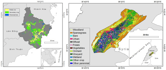
Figure 1.
Cropland maps of Ninh Thuan, Vietnam [34] (left) and of Bekaa, Lebanon [35] (right).
Ninh Thuan is the most drought-prone province in Vietnam [36]. To cope with water shortage throughout the dry season (from Jan to Aug), rainwater is collected during the rainy season (from Aug to Nov) with more than 20 small to medium-size reservoirs. The extension of the cropland area is largest during the winter–spring season, then it reduces during the summer because of water shortage. Moreover, the crop during rainy season can be vulnerable to floods [37].
2.2. Workflow Overview
We summarized the workflow into three main steps: (1) pre-processing, (2) sensors harmonization, and (3) post-processing as illustrated in Figure 2. In the pre-processing step (red dashed line), we converted the TOA images to surface reflectances (SR) also known as bottom-of-atmosphere (BOA) using one AC model, exclude images that have greater than 30% cloud coverage over the studied area, then mask out all identified cloudy pixels. We applied the AC model via Python API, all the other tasks were Code Editor based. Because the BRDF and topographic correction models require digital elevation model (DEM) data, they are applied only when the images had been coregistered. The harmonization step (green dashed line) refers to re-projection, re-scaling, and re-alignment (co-registration) of the L7, L8 and S2 images. Finally, the post-processing step (blue dashed line) stacks all the harmonized images into a database of the GEE assets. This step also calculates composite images (mean) of every 10-day period (dekadal) and exports them to Google Drive, making it a shareable geospatial dataset for non-GEE users. The GEE scripts used in the study and links to the generated harmonized datasets that contain the SR images (bands blue, green, red, nir, swir1, swir2, and ndvi at 30 m) over both areas can be found in the Appendix A.
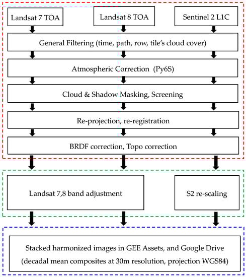
Figure 2.
Workflow of the harmonization in the Google Earth Engine.
2.3. Atmospheric Correction
To reduce residual errors from using different AC methods [24,25], the same AC model called Py6S was applied to all L7, L8 and S2 TOA images. Py6S, was developed by Wilson (2012) [38], is a Python interface of the Second Simulation of the Satellite Signal in the Solar Spectrum or 6S [39] radiative transfer model to reduce the time of setting up numerous input and output data. Results produced from Py6S are the same as the results obtained with 6S [38]. Kotchenova and Vermote, (2007) [40] tested the performance of 6S and found the overall relative error was less than 0.8 percent.
This study implemented Py6S in GEE based on the code shared by Sam Murphy (2019) [41] which was executed via Python API and Docker container. In the model, the view zenith angle was hardcoded to “0”.
2.4. Cloud Mask for Landsat Images
For L7 and L8, cloud and cloud shadow are masked using the Quality Assessment Band (BQA) (30 m resolution) [10], which was generated using the CFMask algorithm. This algorithm has shown the best overall accuracy among many state-of-the-art cloud detection algorithms [42].
2.5. Cloud Mask for Sentinel 2 Images
According to the assessment by Coluzzi et al., (2018) [43], the S2 L1C cloud mask band (QA60, available at 60 m resolution), which is generated based on the blue band (B2) and short-wave infrared bands (B11, B12) [44], generally underestimates the presence of clouds. On the contrary, Clerc et al., (2015), [45] reported that QA60 cloud masks are adjusted to minimize under-detections, which leads to over-detection. In either case, the performance of the L1C cloud mask is low, especially under critical conditions.
In the GEE environment, the authors in Poortinga et al., (2019) [32] applied a cloud scoring algorithm (ee.Algorithms.Landsat.simpleCloudScore [46]) to mask clouds in L8 and S2 images. The algorithm exploits the spectral and thermal properties of bright and cold of clouds that excluding the snow [47]. However, through an exhaustive visual analysis we observed that this Landsat based algorithm did not yield satisfactory results for S2 images over Ninh Thuan, Vietnam. This is likely due to the complex atmospheric condition (e.g., high water vapor content) [43] in Ninh Thuan region and the lack of the thermal band in S2 images.
Following the conclusions of Zupanc (2017) [48], who demonstrated a machine learning approach can outperform current state-of-the-art threshold-based cloud detection algorithms such as Fmask, Sen2Cor, or even MAJA (a multi-temporal approach for cloud detection [49]), this study applied a supervised classification using the QA60 band as covariate to identify cloud contaminated pixels. For every S2 scene, we trained a random forest classifier (ee.Classifier.randomForest()) using stratified random sampling (ee.Image.stratifiedSample()) and the QA60 band was used as the ‘classBand’ argument [50,51]. The stratified sampling function extracted 10 random points from each class contained in the QA60 band which has three classes including ‘opaque clouds’ class (pixel value = 1024), ‘cirrus clouds’ class (pixel value = 2048), and non-cloud-cirrus class (pixel value = 0). In addition, we used a threshold of below than 0.5 for the Normalized Difference Snow Index (NDSI) to prevent snow from being masked [32]. We used a thorough visual inspection to check the performance of this procedure, which showed promising results in such complicated atmospheric conditions like the observed in Ninh Thuan, Vietnam. Figure A1 demonstrated how the cloud was masked in a cloudy S2 scene over Ninh Thuan, Vietnam.
2.6. Cloud Shadow Detection
Cloud shadows can be predicted using the cloud’s shape, height and sun position at that time [52]. However, this method depends on the cloud identification ability and poses large uncertainty while projecting the cloud’s shadow on the earth’s surface. This study used a Temporal Dark Outlier Mask (TDOM) method which greatly improves the detection of cloud shadow by obtaining dark pixel anomaly [47]. The TDOM method is based on the idea that cloud shadows appear and disappear quickly as the cloud moves. The implementation of TDOM in GEE was adapted from Poortinga et al., (2019) [32].
2.7. Co-Registration between Landsat and Sentinel 2 Images
The misalignment (or misregistration) between L8 and S2 images varied geographically and can exceed 38 m [19] which is mainly due to the residual geolocation errors in the L8 framework which were based upon the Global Land Survey images. In GEE, we used displacement() function to measure the displacement between two overlapped S2 and L8 images which were captured at the same time over the studied regions. Then, the displace() function is used to align (“rubber-sheet” technique) the L8 image with the S2 image [53]. Because the L8-S2 misalignment is reported stable for a given area and additionally, the S2 absolute geodetic accuracy is better than L8 [19], this study aligned all Landsat images (same PATH, ROW) using a common base S2 [54]. We also assumed that the misalignment among the same satellite images is neglectable. The co-alignment step described here is purely an image processing technique. It differs from geo-referencing or geo-correcting which involves aligning images to the correct geographic location through ground control points. At the moment, GEE documentation does not explain clearly the underlying of displacement() and displace() algorithms; however, the authors in Gao et al., (2009) [55] described in great detail a similar tool called AROP which is an open-source package designed specifically for registration and orthorectification of Landsat and Landsat-like data.
2.8. Re-Projection and Scaling
Because each band can have a different scale and projection [56], band’s projection was therefore transformed according to the red band of S2 (WGS84) and band’s resolution was rescaled to 30 m using ‘bicubic’ interpolation [57,58]. In fact, unlike other GIS and image processing platforms, the scale of analysis in GEE is quite flexible; the scale is determined from the output, rather than the input via a pyramiding policy [59].
2.9. BRDF Correction
The Bidirectional Reflectance Distribution Functions (BRDF) model is applied to reduce the directional effects due to the differences in solar and view angles between L7, L8 and S2 [11]. The implementation of BRDF correction in GEE was developed by Poortinga et al., (2019) [32] based on results from different studies [29,30]. This BRDF correction is MODIS-based fixed coefficients c-factor, originally developed for Landsat but proven that it works for S2 as well [21,29,30]. The view angle is set to nadir and the illumination is set based on the center latitude of the tile [11].
2.10. Topographic Correction
Topographic correction accounts for variations in reflectance due to slope, aspect, and elevation. It is not always required but can be essential in mountainous or rugged terrain [60,61]. The implementation of topographic correction in GEE was developed by Poortinga et al., (2019) [32]. The method is based on the modified Sun-Canopy-Sensor Topographic Correction as described in [31]. The DEM used is the SRTM V3 product (30 m SRTM Plus) which includes a void-filling process using open-source data (ASTER GDEM2, GMTED2010, and NED) provided by NASA JPL [62].
2.11. Band Adjustment
Although efforts have been made in the radiometric and geometric calibration of the Landsat and S2 missions so that their bands could be compatible [20], small spectral differences still exist [11,20,33]. We adjusted the six Landsat bands (blue, green, red, nir, swir1, and swir2) using cross-sensor transformation coefficients (Table 1) derived from Chastain et al., (2019) [33]. Chastain et al., (2019) [33] used absolute difference metrics and major axis linear regression analysis over 10,000 image pairs across the conterminous United States to obtain these transformation coefficients.
2.12. Cropland Detection Using Harmonic Analysis of Time Series
The extended cropland land cover is valuable for the Ninh Thuan province’s Irrigation Management Company (IMC) to calculate water distribution volume and predict water demand for the next season. However, because of seasonal variation, mixed crop rotation and data scarcity, it is difficult for the province to obtain the up-to-date and accurate seasonal extended croplands extension. To improve the accuracy of cropland detection, it is desirable to apply a temporal signature approach that can utilize data acquired at different growth stages; and therefore, increasing the dimensionality of information [63]. As the harmonic (or Fourier) analysis has proven to be useful in characterizing seasonal cycles and variation in land used/land cover types [9,64,65,66,67], this study applied an harmonic analysis on dense NDVI time series, obtained from the harmonized dataset (L7, L8, and S2), to mapping seasonal croplands in Ninh Thuan during 2018. As illustrated in Figure 1 in [65], harmonic (Fourier) analysis permits a complex curve to be expressed as the sum of a series of cosine waves and an additive term. Each wave is defined by a unique amplitude and a phase angle where the amplitude value is half the height of a wave, and the phase angle (or simply, phase) defines the offset between the origin and the peak of the wave over the range 0–2 . Therefore, high seasonal variation in NDVI of crop pixels will be characterized by high amplitude values and phase angles.
3. Results and Discussion
3.1. Design of the Evaluation Experiments
This study used several transformation models from other studies, for example, BRDF and topographic correction models from Poortinga et al., (2019) [32]; band adjustment coefficients from Chastain et al., (2019) [33]; and image co-registration built-in function in the GEE [53].
However, some studies suggested that site-specific models may be required for specific areas of study due to inconsistent regression coefficient values obtained across different study areas [21,68,69].
In addition, the sequences of processing steps as described in Figure 2 could be evaluated to generate the most optimized results. For example, we could compute band adjustment at the beginning of the workflow because the cross-sensor transformation coefficients that we used (Table 1) were calculated for TOA images. This adjustment might also improve the co-registration step later on since it is based on the comparison of the values of the pixels in two images. Therefore, it is desirable to understand and evaluate the effects of each processing/transformation step and compare the initial images with the final results. In this study, we applied several tests on two overlapped S2 and L8 images which were captured at the same time over the studied regions, before and after each processing step. Rectangular areas without cloud, cirrus, or saturated pixels were selected for analysis.
Although 30 m is the spatial resolution for every band in the harmonized data set, we evaluated the effect of each processing/transformation at 10 m resolution, we believe that at 30 m, the evaluation could have yielded better results.
The image IDs, date, and the acquisition time of the tested images are presented in Table 2. In Section 3.2, we estimated the reduction in sensor misregistration, while in Section 3.3, we calculated the spatial Pearson’s correlation for each band, and finally, in Section 3.4, we assessed the temporal correlation of NDVI time series.
Table 2.
Overlapped S2 and L8 images selected for performance evaluation.
3.2. Reducing the Sensors Misregistration
Figure 3 shows the offset differences in the tested areas, measured by the magnitude of the vector formed by dX and dY [53] before and after the overlapped pair of L8-S2 images were co-registered using the method described in Section 2.7. For Bekaa, the offset differences were reduced substantially from 22–32 m meters to less than 8 m (less than 2 m on average). For Ninh Thuan, Vietnam, the offset differences were reduced from 12 m (maximum) to less than 2 m in most of the pixels. These results are in agreement with Storey et al., (2016) [19] who also found misalignments that geographically varied between L8-S2. Further analysis (see Table 3) showed that the co-registration step contributed the most to the improvement in band-to-band spatial correlation.
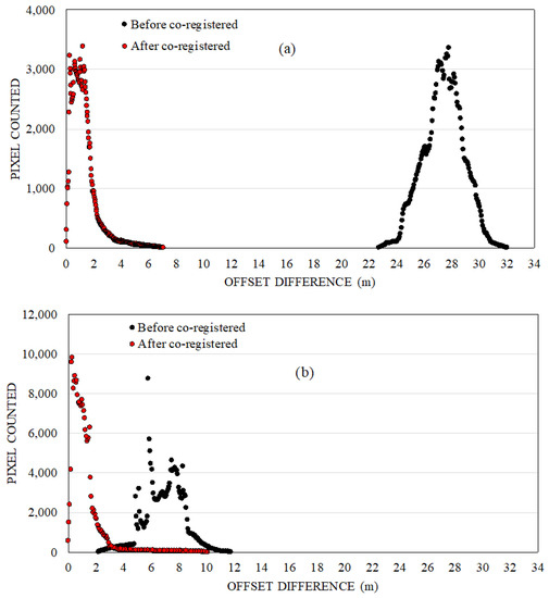
Figure 3.
Offset differences per-pixel between L8 and S2 in the tested areas: (a) Bekaa, Lebanon and (b) Ninh Thuan, Vietnam, measured by the magnitude of the vector formed by dX and dY. The black dots represent the offset distances between the original images of L8 and S2, while the red dots represent the offset distances when the images were co-registered.
Table 3.
L8–S2 cross-comparison of the Pearson correlation values (r) in the red, nir, and ndvi bands for each processing/transformation step when the process was applied over the flat area (a) and the mountainous area (b).
3.3. Improving Band-to-Band Spatial Correlation
We analyzed the band-to-band correlation over two separated domains, a flat agricultural area (Figure 4a), and a mountainous area (Figure 4b). Each domain has an extent of 0.3 km, without cloud, cirrus, or saturated pixels.
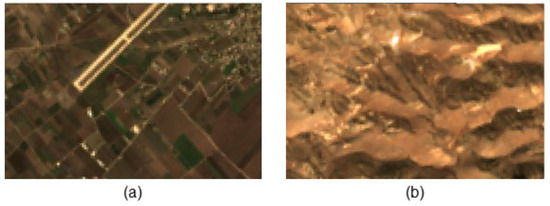
Figure 4.
A flat agricultural area (a), and a mountainous area (b) in Bekaa, Lebanon, represented by true-color composites of the Landsat 8, used for L8-S2 band-to-band correlation analysis. Each domain has an area of 0.3 km, without cloud, cirrus or saturated pixels.
Table 3 compares the Pearson correlation values (r) of the red, nir, and ndvi bands when each processing/transformation step was applied (P0 to P5), over both the flat and the mountainous area. From P1, we rescaled L8 to the same resolution with S2 (10 m) using bicubic interpolation function in GEE. After each processing step, NDVI was calculated from the processed band Red and Nir. For the flat area, correlation values increased substantially from 0.67, 0.75, 0.79 to 0.93, 0.95, 0.96 in the red, nir, and ndvi bands, respectively. For the mountainous area, r increased from 0.56, 0.45, 0.63 to 0.77, 0.72, 0.80 in the red, nir, and ndvi bands, respectively. Table 3 also indicates that the co-registration step (P3) contributed the most in the band-to-band spatial correlation improvement.
The correlation was higher in the flat area compared to the mountainous area, likely due to the impacts of untreated hill shadow or hill’s slope. This result is in agreement with Colby, (1991) [60] and Vanonckelen et al., (2013) [61] who emphasized the importance of properly topographic correction in mountainous or rugged terrain. In addition, in Table 3, while both Red and nir correlations improved with topo correction (step P4) over the mountainous region, the NDVI correlation decreased. Based on this observation, we suggeste that further analysis should be made to better optimize results for the mountainous area. We will discuss some possible solutions in Section 3.4.
The comparison of the differences before and after processing in all bands are indicated in Figure 5. This is an analysis over the flat domain in Bekaa (Figure 4a) using the first pair of L8-S2 images provided in Table 2. Figure 5 presented per-pixel scatter plots of all seven bands (blue, green, red, nir, swir1, swir2, and ndvi), compared (using the r, bias, and RMSE) before and after the overlapped L8-S2 images were harmonized. These plots showed all bands are in good agreement. Band SWIR1 reached the highest correlation (r = 0.97) and band Blue has the lowest (r = 0.87).
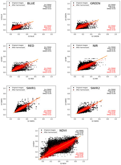
Figure 5.
Scatters plots of all seven bands per pixel (blue, green, red, nir, swir1, swir2, and ndvi) for the flat domain in Bekaa, provided N (total number of the pixels), r, bias, and RMSE (Root Mean Square Error). The black and red dots represent the images before and after the overlapped L8-S2 images were harmonized.
3.4. Affect of Band Adjustment to Temporal Correlation in NDVI Time Series
Figure 6 showes NDVI time series at a typical crop pixel (lat = 36.01, long = 33.83) before and after the application of the band adjustment. We observe that before the band adjustment, the NDVI values of L8 were systematically lower than those of S2; however, after the band adjustment, the two datasets matched chronologically. The third one shows the final harmonized ndvi time series which used data from all sensors. There are gaps in the time series because cloudy covered images were automatically eliminated from the process.
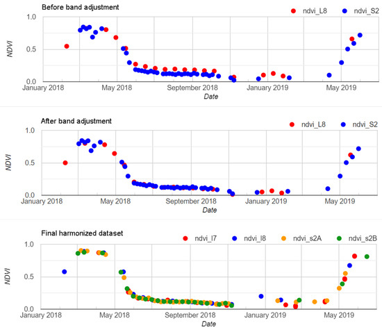
Figure 6.
The first two plots (from top to bottom) show the temporal NDVI time series over a typical crop pixel in Bekaa, Lebanon (lat = 36.01, long = 33.83) before and after band adjustment, respectively. The last image shows the harmonized NDVI time series from all sensors. There are gaps in the time series due to the removal of the cloudy images.
As previously reported in Section 3.3 and Table 3, the Pearson cross-correlation of the different bands is low in the mountainous region due to the impacts of the hill’s slope or remaining of untreated hill shadow or unknown reasons. This problem is further visualized in Figure 7, which showed the NDVI time series of a pixel located in a mountainous area (lat = 36.04, long = 33.81). After the processing, Landsat’s NDVI values were seen systematically lower than those of S2.
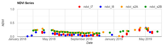
Figure 7.
NDVI time series of a pixel located in a mountainous area in Bekaa (lat = 36.04, long = 33.81). After the harmonization process, the Landsat’s NDVI values were systematically lower than those of S2.
These results suggestes that we may need to apply different treatment for the mountainous or rugged terrain areas than in the flat agricultural areas. The domain for mountainous regions could be defined using slope or aspect threshold derived from DEM data. Modifying the band adjustment coefficients could play an important role. One can re-calculate these coefficients so that they are more adaptable to these particular studied areas.
3.5. Assessing the Dynamic Cropland Variation in Ninh Thuan, Vietnam
As described in Section 2.12 and following the methodology described in Ghazaryan et al., (2018) [9], combined with implementation of the harmonic model in GEE by Nicholas Clinton, (2017) [70], we fitted the time series of NDVI data in every pixel. Figure 8 shows the NDVI time series and the fitted values of regions that have one crop (unimodal greeness pattern), two crops (bimodal greeness pattern), and three crops (trimodal greeness pattern) per year in Ninh Thuan region. The exact locations of the plotted pixels are labeled as (a), (b), (c) in Figure 9. The phase (angle from the starting point to the cycle’s peak) and amplitude (half of the cycle’s height) values, which were derived from the harmonic models, were used to express the temporal signature of NDVI.
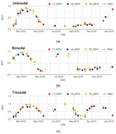
Figure 8.
Detected unimodal (a), bimodal (b) and trimodal (c) shapes in the temporal NDVI patterns of different paddy rice areas in Ninh Thuan during 2018. The fitted values (smaller green dots) were used to calculate the phase and amplitude of the cycles.
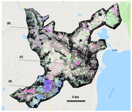
Figure 9.
Cropland variation characterized by a R-G-B false composite images from amplitude, phase (of the first harmonic term), and max-NDVI values. This map highlighted the croplands in Ninh Thuan during 2018 as colored pixels (high phase and amplitude) and other types of land as grey/dark pixels (low phase/amplitude). (a–c) are regions corresponding to the unimodal, bimodal, and trimodal time series presented in Figure 8.
Since the first harmonic term represents the annual cycle [64], the cropland’s variation was identified using a composite image of phase, amplitude (of the first harmonic term), and the max NDVI (Figure 9). Because NDVI at cropland pixels were characterized with high temporal variation, high angle or sharp turn at the peak of crop growth, and high max NDVI values, were highlighted in Figure 9 as bright colored pixels, while black or gray pixels represent non-cropland classes.
Although the derived amplitude and phase values are sufficient to differentiate croplands versus non-cropland pixels, Max-NDVI was added as a third band to give us an additional option to highlight the color of the cropland pixels by scale up their band’s values. Furthermore, Max-NDVI is useful in a decision rule set to further separate crop types [9]. However, in this study, we only have interest in detecting the main croplands.
4. Conclusions
In the presented study, we demonstrated a robust workflow in GEE to generate harmonized L7, L8, and S2 images for two agricultural schemes in Bekaa, Lebanon, and Ninh Thuan, Vietnam. We also evaluated the performance of several pre-processing steps needed for the harmonization including image co-registration, BRDF correction, topographic correction, and band adjustment. Although, the band adjustment showed little impact on the Pearson cross-correlation results; it is an important process to match temporal spectral time series. The offset difference between L8 and S2 images in the Bekaa region was as large as 32 m, and if not treated, it poses a great impact on the quality of the harmonized dataset. Although a topographic correction model was applied, the lowest performance was observed in mountainous areas.
The use of a high amount of observations also omits the need for data smoothing techniques. We also demonstrated an application of the harmonized dataset by mapping the extended cropland via harmonic analysis for Ninh Thuan province in 2018.
Author Contributions
M.D.N. contributed to the study’s design, data analysis, programming and writing the manuscript, O.M.B.-V. and L.R. made contributions to the design, statistical analyses, writing, and supervised all stages of the study, O.M.B.-V., L.R., D.D.B., and P.T.N. participated in the discussion of the results. All authors read and approved the submitted manuscript.
Funding
This research received no external funding.
Acknowledgments
The author acknowledges the support by Vingroup Innovation Foundation (VINIF) with the project code VINIF.2019.DA17 and the Vietnam National Foundation for Science and Technology Development (NAFOSTED) under the Grant No. NE/S002847/1. The author acknowledges comments and expertise from colleagues at eLEAF B.V. (Wageningen, The Netherlands) that greatly improved this research. We thank the three anonymous reviewers for their insights and constructive criticism that helped to improve the final version of this manuscript.
Conflicts of Interest
The authors declare no conflict of interest.
Appendix A
Harmonized datasets that contain SR images (bands blue, green, red, nir, swir1, swir2, and ndvi at 30 m) over the two studied sites, which are provided for public usage and testing. Data link (Google drive): https://drive.google.com/open?id=1no0MmpL_WA8BWzFRmmUWGPMt-JYMtI-P. GEE app to inspect the NDVI time series and the detected croplands in Ninh Thuan: https://ndminhhus.users.earthengine.app/view/cropninhthuan2019. All GEE scripts used in the study are documented at https://github.com/ndminhhus/geeguide.

Figure A1.
Demonstration of cloud masking steps. (a) cloudy true color image, (b) cloud and cirrus masked (yellow) using only QA60 Band, (c) cloud mask using combination of Red and Aerosol Band (B4 & B1), (d) cloud mask using random forest classification, band QA60 was used as training field, (e) final cloud mask combining all masks together. This scene was acquired by Sentienl 2B on 12 May 2019 over Ninh Thuan, Vietnam (id = COPERNICUS/S2/20190513T030549_20190513T032056_T49PBN).
References
- Bégué, A.; Arvor, D.; Bellon, B.; Betbeder, J.; De Abelleyra, D.; PD Ferraz, R.; Lebourgeois, V.; Lelong, C.; Simões, M.; Verón, S.R. Remote sensing and cropping practices: A review. Remote Sens. 2018, 10, 99. [Google Scholar] [CrossRef]
- Cheng, T.; Yang, Z.; Inoue, Y.; Zhu, Y.; Cao, W. Preface: Recent advances in remote sensing for crop growth monitoring. Remote Sens. 2016, 8, 116. [Google Scholar] [CrossRef]
- Strand, H.; Höft, R.; Strittholt, J.; Miles, L.; Horning, N.; Fosnight, E.; Turner, W. Sourcebook on Remote Sensing and Biodiversity Indicators, CBD Technical Series No. 32; Secretariat of the Convention on Biological Diversity: Montreal, QC, Canada, 2007. [Google Scholar]
- He, M.; Kimball, J.; Maneta, M.; Maxwell, B.; Moreno, A.; Beguería, S.; Wu, X. Regional crop gross primary productivity and yield estimation using fused landsat-MODIS data. Remote Sens. 2018, 10, 372. [Google Scholar] [CrossRef]
- Yang, D.; Su, H.; Zhan, J. MODIS-Landsat Data Fusion for Estimating Vegetation Dynamics—A Case Study for Two Ranches in Southwestern Texas. In Proceedings of the 1st International Electronic Conference on Remote Sensing, 22 June–5 July 2015. [Google Scholar]
- Hansen, M.C.; Loveland, T.R. A review of large area monitoring of land cover change using Landsat data. Remote Sens. Environ. 2012, 122, 66–74. [Google Scholar] [CrossRef]
- Whitcraft, A.; Becker-Reshef, I.; Justice, C. A framework for defining spatially explicit earth observation requirements for a global agricultural monitoring initiative (GEOGLAM). Remote Sens. 2015, 7, 1461–1481. [Google Scholar] [CrossRef]
- Hilker, T.; Wulder, M.A.; Coops, N.C.; Seitz, N.; White, J.C.; Gao, F.; Masek, J.G.; Stenhouse, G. Generation of dense time series synthetic Landsat data through data blending with MODIS using a spatial and temporal adaptive reflectance fusion model. Remote Sens. Environ. 2009, 113, 1988–1999. [Google Scholar] [CrossRef]
- Ghazaryan, G.; Dubovyk, O.; Löw, F.; Lavreniuk, M.; Kolotii, A.; Schellberg, J.; Kussul, N. A rule-based approach for crop identification using multi-temporal and multi-sensor phenological metrics. Eur. J. Remote Sens. 2018, 51, 511–524. [Google Scholar] [CrossRef]
- USGS. US Geological Survey (USGS) Landsat Collection 1 Level-1 Quality Assessment Band. 2019. Available online: https://www.usgs.gov/land-resources/nli/landsat/landsat-collection-1-level-1-quality-assessment-band?qt-science_support_page_related_con=0#qt-science_support_page_related_con (accessed on 9 September 2019).
- Claverie, M.; Ju, J.; Masek, J.G.; Dungan, J.L.; Vermote, E.F.; Roger, J.C.; Skakun, S.V.; Justice, C. The Harmonized Landsat and Sentinel-2 surface reflectance data set. Remote Sens. Environ. 2018, 219, 145–161. [Google Scholar] [CrossRef]
- Claverie, M.; Demarez, V.; Duchemin, B.; Hagolle, O.; Ducrot, D.; Marais-Sicre, C.; Dejoux, J.F.; Huc, M.; Keravec, P.; Béziat, P.; et al. Maize and sunflower biomass estimation in southwest France using high spatial and temporal resolution remote sensing data. Remote Sens. Environ. 2012, 124, 844–857. [Google Scholar] [CrossRef]
- Skakun, S.; Vermote, E.; Roger, J.C.; Franch, B. Combined use of Landsat-8 and Sentinel-2A images for winter crop mapping and winter wheat yield assessment at regional scale. AIMS Geosci. 2017, 3, 163. [Google Scholar] [CrossRef]
- Boschetti, L.; Roy, D.P.; Justice, C.O.; Humber, M.L. MODIS–Landsat fusion for large area 30 m burned area mapping. Remote Sens. Environ. 2015, 161, 27–42. [Google Scholar] [CrossRef]
- Ma, J.; Zhang, W.; Marinoni, A.; Gao, L.; Zhang, B. An improved spatial and temporal reflectance unmixing model to synthesize time series of landsat-like images. Remote Sens. 2018, 10, 1388. [Google Scholar] [CrossRef]
- Wang, Q.; Zhang, Y.; Onojeghuo, A.O.; Zhu, X.; Atkinson, P.M. Enhancing spatio-temporal fusion of modis and landsat data by incorporating 250 m modis data. IEEE J. Sel. Top. Appl. Earth Obs. Remote Sens. 2017, 10, 4116–4123. [Google Scholar] [CrossRef]
- Dong, J.; Zhuang, D.; Huang, Y.; Fu, J. Advances in multi-sensor data fusion: Algorithms and applications. Sensors 2009, 9, 7771–7784. [Google Scholar] [CrossRef] [PubMed]
- Behnia, P. Comparison between four methods for data fusion of ETM+ multispectral and pan images. Geo-Spat. Inf. Sci. 2005, 8, 98–103. [Google Scholar] [CrossRef]
- Storey, J.; Roy, D.P.; Masek, J.; Gascon, F.; Dwyer, J.; Choate, M. A note on the temporary misregistration of Landsat-8 Operational Land Imager (OLI) and Sentinel-2 Multi Spectral Instrument (MSI) imagery. Remote Sens. Environ. 2016, 186, 121–122. [Google Scholar] [CrossRef]
- Barsi, J.A.; Alhammoud, B.; Czapla-Myers, J.; Gascon, F.; Haque, M.O.; Kaewmanee, M.; Leigh, L.; Markham, B.L. Sentinel-2A MSI and Landsat-8 OLI radiometric cross comparison over desert sites. Eur. J. Remote Sens. 2018, 51, 822–837. [Google Scholar] [CrossRef]
- Zhang, H.K.; Roy, D.P.; Yan, L.; Li, Z.; Huang, H.; Vermote, E.; Skakun, S.; Roger, J.C. Characterization of Sentinel-2A and Landsat-8 top of atmosphere, surface, and nadir BRDF adjusted reflectance and NDVI differences. Remote Sens. Environ. 2018, 215, 482–494. [Google Scholar] [CrossRef]
- Gao, F.; He, T.; Masek, J.G.; Shuai, Y.; Schaaf, C.B.; Wang, Z. Angular effects and correction for medium resolution sensors to support crop monitoring. IEEE J. Sel. Top. Appl. Earth Obs. Remote Sens. 2014, 7, 4480–4489. [Google Scholar] [CrossRef]
- Franch, B.; Vermote, E.; Skakun, S.; Roger, J.C.; Santamaria-Artigas, A.; Villaescusa-Nadal, J.L.; Masek, J. Towards Landsat and Sentinel-2 BRDF normalization and albedo estimation: A case study in the Peruvian Amazon forest. Front. Earth Sci. 2018, 6, 185. [Google Scholar] [CrossRef]
- Ilori, C.O.; Pahlevan, N.; Knudby, A. Analyzing Performances of Different Atmospheric Correction Techniques for Landsat 8: Application for Coastal Remote Sensing. Remote Sens. 2019, 11, 469. [Google Scholar] [CrossRef]
- Doxani, G.; Vermote, E.; Roger, J.C.; Gascon, F.; Adriaensen, S.; Frantz, D.; Hagolle, O.; Hollstein, A.; Kirches, G.; Li, F.; et al. Atmospheric correction inter-comparison exercise. Remote Sens. 2018, 10, 352. [Google Scholar] [CrossRef]
- Kumar, L.; Mutanga, O. Google Earth Engine applications since inception: Usage, trends, and potential. Remote Sens. 2018, 10, 1509. [Google Scholar] [CrossRef]
- Gorelick, N.; Hancher, M.; Dixon, M.; Ilyushchenko, S.; Thau, D.; Moore, R. Google Earth Engine: Planetary-scale geospatial analysis for everyone. Remote Sens. Environ. 2017, 202, 18–27. [Google Scholar] [CrossRef]
- Kennedy, R.; Yang, Z.; Gorelick, N.; Braaten, J.; Cavalcante, L.; Cohen, W.; Healey, S. Implementation of the LandTrendr Algorithm on Google Earth Engine. Remote Sens. 2018, 10, 691. [Google Scholar] [CrossRef]
- Roy, D.P.; Li, J.; Zhang, H.K.; Yan, L.; Huang, H.; Li, Z. Examination of Sentinel-2A multi-spectral instrument (MSI) reflectance anisotropy and the suitability of a general method to normalize MSI reflectance to nadir BRDF adjusted reflectance. Remote Sens. Environ. 2017, 199, 25–38. [Google Scholar] [CrossRef]
- Roy, D.P.; Zhang, H.; Ju, J.; Gomez-Dans, J.L.; Lewis, P.E.; Schaaf, C.; Sun, Q.; Li, J.; Huang, H.; Kovalskyy, V. A general method to normalize Landsat reflectance data to nadir BRDF adjusted reflectance. Remote Sens. Environ. 2016, 176, 255–271. [Google Scholar] [CrossRef]
- Soenen, S.A.; Peddle, D.R.; Coburn, C.A. SCS+ C: A modified sun-canopy-sensor topographic correction in forested terrain. IEEE Trans. Geosci. Remote Sens. 2005, 43, 2148–2159. [Google Scholar] [CrossRef]
- Poortinga, A.; Tenneson, K.; Shapiro, A.; Nquyen, Q.; San Aung, K.; Chishtie, F.; Saah, D. Mapping Plantations in Myanmar by Fusing Landsat-8, Sentinel-2 and Sentinel-1 Data along with Systematic Error Quantification. Remote Sens. 2019, 11, 831. [Google Scholar] [CrossRef]
- Chastain, R.; Housman, I.; Goldstein, J.; Finco, M. Empirical cross sensor comparison of Sentinel-2A and 2B MSI, Landsat-8 OLI, and Landsat-7 ETM+ top of atmosphere spectral characteristics over the conterminous United States. Remote Sens. Environ. 2019, 221, 274–285. [Google Scholar] [CrossRef]
- NinhThuan-DONRE. Shapefiles “Paddy Rice, Secondary Crop and Perennial Trees in Ninh Thuan, Surveyed 2015”; Proj. Data; Department of Natural Resources and Environment: Ninh Thuan, Vietnam, 2015.
- eLEAF, B.V. Summary Methodology of Level 3 Land Cover Mapping, L3 Class Description. Proj. Data 2015, 4–6. [Google Scholar]
- VAWR. Report “Strengthening the Agro-Climatic Information System to Improve the Agricultural Drought Monitoring and Early Warning System in Vietnam (NEWS), Pilot Study in the Ninh Thuan Province”; Project Inception Report; Vietnam Academy for Water Resources: Hanoi, Vietnam, 2017. [Google Scholar]
- NinhThuan-MPI. Report “Review and Update Irrigation Planning of the Ninh Thuan Province to 2020, Vision to 2030 under Climate Change Scenario”; Project Report; Department of Planning and Investment: Ninh Thuan, Vietnam, 2015.
- Wilson, R. Py6S: A Python Interface to the 6S Radiative Transfer. 2012. Available online: http://rtwilson.com/academic/Wilson_2012_Py6S_Paper.pdf (accessed on 9 September 2019).
- Vermote, E.F.; Tanré, D.; Deuze, J.L.; Herman, M.; Morcette, J.J. Second simulation of the satellite signal in the solar spectrum, 6S: An overview. IEEE Trans. Geosci. Remote Sens. 1997, 35, 675–686. [Google Scholar] [CrossRef]
- Kotchenova, S.Y.; Vermote, E.F. Validation of a vector version of the 6S radiative transfer code for atmospheric correction of satellite data. Part II. Homogeneous Lambertian and anisotropic surfaces. Appl. Opt. 2007, 46, 4455–4464. [Google Scholar] [CrossRef]
- Sam, M. Atmospheric Correction of Sentinel 2 Imagery in Google Earth Engine Using Py6S. 2018. Available online: https://github.com/samsammurphy/gee-atmcorr-S2 (accessed on 9 September 2019).
- Foga, S.; Scaramuzza, P.L.; Guo, S.; Zhu, Z.; Dilley, R.D., Jr.; Beckmann, T.; Schmidt, G.L.; Dwyer, J.L.; Hughes, M.J.; Laue, B. Cloud detection algorithm comparison and validation for operational Landsat data products. Remote Sens. Environ. 2017, 194, 379–390. [Google Scholar] [CrossRef]
- Coluzzi, R.; Imbrenda, V.; Lanfredi, M.; Simoniello, T. A first assessment of the Sentinel-2 Level 1-C cloud mask product to support informed surface analyses. Remote Sens. Environ. 2018, 217, 426–443. [Google Scholar] [CrossRef]
- ESA. Level-1C Cloud Masks-Sentinel-2 MSI Technical Guide-Sentinel Online. 2019. Available online: https://sentinel.esa.int/web/sentinel/technical-guides/sentinel-2-msi/level-1c/cloud-masks (accessed on 9 September 2019).
- Clerc, S.; Devignot, O.; Pessiot, L. S2 MPC TEAM S2 MPC Data Quality Report-2015-11-30. 2015. Available online: https://sentinels.copernicus.eu/documents/247904/685211/Sentinel-2+Data+Quality+Report (accessed on 9 September 2019).
- GEE. Landsat Algorithms in Google Earth Engine API. 2019. Available online: https://developers.google.com/earth-engine/landsat (accessed on 9 September 2019).
- Housman, I.; Chastain, R.; Finco, M. An Evaluation of Forest Health Insect and Disease Survey Data and Satellite-Based Remote Sensing Forest Change Detection Methods: Case Studies in the United States. Remote Sens. 2018, 10, 1184. [Google Scholar] [CrossRef]
- Zupanc, A. Improving Cloud Detection with Machine Learning. 2017. Available online: https://medium.com/sentinel-hub/improving-cloud-detection-with-machine-learning-c09dc5d7cf13 (accessed on 9 September 2019).
- Hagolle, O.; Huc, M.; Pascual, D.V.; Dedieu, G. A multi-temporal method for cloud detection, applied to FORMOSAT-2, VENμS, LANDSAT and SENTINEL-2 images. Remote Sens. Environ. 2010, 114, 1747–1755. [Google Scholar] [CrossRef]
- Breiman, L. Random forests. Mach. Learn. 2001, 45, 5–32. [Google Scholar] [CrossRef]
- GEE. Supervised Classification in Google Earth Engine API. 2019. Available online: https://developers.google.com/earth-engine/classification (accessed on 9 September 2019).
- Hollstein, A.; Segl, K.; Guanter, L.; Brell, M.; Enesco, M. Ready-to-use methods for the detection of clouds, cirrus, snow, shadow, water and clear sky pixels in Sentinel-2 MSI images. Remote Sens. 2016, 8, 666. [Google Scholar] [CrossRef]
- GEE. Registering Images in Google Earth Engine API. 2019. Available online: https://developers.google.com/earth-engine/register (accessed on 9 September 2019).
- Claverie, M.; Jeffrey, G.M.; Junchang, J.; Jennifer, L.D. Harmonized Landsat-8 Sentinel-2 (HLS) Product User’s Guide. 2017. Available online: https://hls.gsfc.nasa.gov/wp-content/uploads/2017/08/HLS.v1.3.UserGuide_v2-1.pdf (accessed on 9 September 2019).
- Gao, F.; Masek, J.G.; Wolfe, R.E. Automated registration and orthorectification package for Landsat and Landsat-like data processing. J. Appl. Remote Sens. 2009, 3, 033515. [Google Scholar]
- GEE. Projections in Google Earth Engine API. 2019. Available online: https://developers.google.com/earth-engine/projections (accessed on 9 September 2019).
- GEE. Resampling and Reducing Resolution in Google Earth Engine API. 2019. Available online: https://developers.google.com/earth-engine/resample (accessed on 9 September 2019).
- Keys, R. Cubic convolution interpolation for digital image processing. IEEE Trans. Acoust. Speech Signal Process. 1981, 29, 1153–1160. [Google Scholar] [CrossRef]
- GEE. Scale in Google Earth Engine API. 2019. Available online: https://developers.google.com/earth-engine/scale (accessed on 9 September 2019).
- COLBY, J. Topographic normalization in rugged terrain. Photogramm. Eng. Remote Sens. 1991, 57, 531–537. [Google Scholar]
- Vanonckelen, S.; Lhermitte, S.; Van Rompaey, A. The effect of atmospheric and topographic correction methods on land cover classification accuracy. Int. J. Appl. Earth Obs. Geoinf. 2013, 24, 9–21. [Google Scholar] [CrossRef]
- GEE. SRTM Digital Elevation Data 30m. 2019. Available online: https://developers.google.com/earth-engine/datasets/catalog/USGS_SRTMGL1_003 (accessed on 9 September 2019).
- Dutta, S.; Patel, N.; Medhavy, T.; Srivastava, S.; Mishra, N.; Singh, K. Wheat crop classification using multidate IRS LISS-I data. J. Indian Soc. Remote Sens. 1998, 26, 7–14. [Google Scholar] [CrossRef]
- Jakubauskas, M.E.; Legates, D.R.; Kastens, J.H. Crop identification using harmonic analysis of time-series AVHRR NDVI data. Comput. Electron. Agric. 2002, 37, 127–139. [Google Scholar] [CrossRef]
- Jakubauskas, M.E.; Legates, D.R.; Kastens, J.H. Harmonic analysis of time-series AVHRR NDVI data. Photogramm. Eng. Remote Sens. 2001, 67, 461–470. [Google Scholar]
- Jakubauskas, M.; Legates, D.R. Harmonic analysis of time-series AVHRR NDVI data for characterizing US Great Plains land use/land cover. Int. Arch. Photogramm. Remote Sens. 2000, 33, 384–389. [Google Scholar]
- Shumway, R.H.; Stoffer, D.S. Time Series Analysis and Its Applications: With R Examples; Springer: New York, NY, USA, 2017. [Google Scholar]
- Mandanici, E.; Bitelli, G. Preliminary comparison of sentinel-2 and landsat 8 imagery for a combined use. Remote Sens. 2016, 8, 1014. [Google Scholar] [CrossRef]
- Flood, N. Comparing Sentinel-2A and Landsat 7 and 8 using surface reflectance over Australia. Remote Sens. 2017, 9, 659. [Google Scholar] [CrossRef]
- Nick, C. Time Series Analysis in Earth Engine. 2017. Available online: https://goo.gl/lMwd2Y (accessed on 9 September 2019).
© 2020 by the authors. Licensee MDPI, Basel, Switzerland. This article is an open access article distributed under the terms and conditions of the Creative Commons Attribution (CC BY) license (http://creativecommons.org/licenses/by/4.0/).