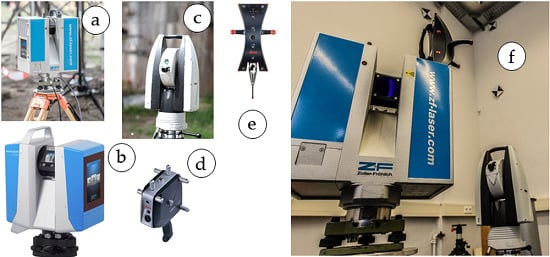
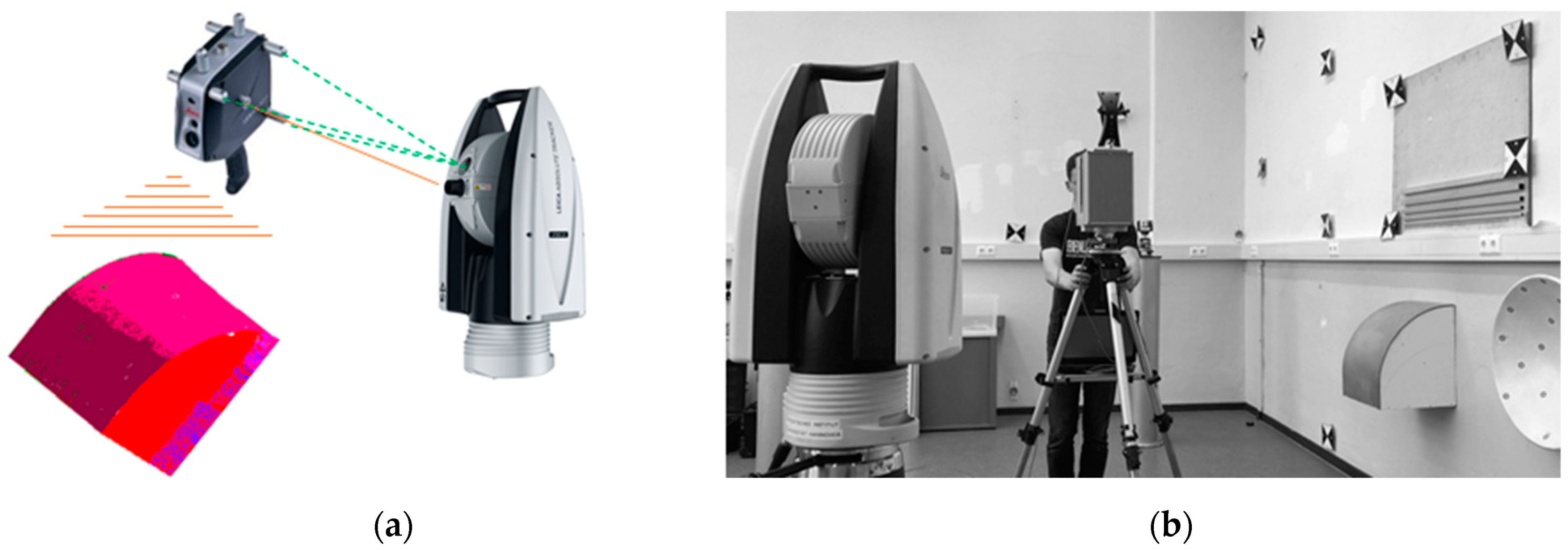
Figure 1.
Sensors used at the Geodetic Institute Hannover (GIH) (
a) Z + F Imager 5010X; (
b) Z + F Imager 5016 (
zf-laser.com), (
c) Leica AT960 LR; (
d) Leica T-Scan 5 (
metrology.leica-geosystems.com); (
e) Leica T-Probe (
www.hexagonmi.com); (
f) k-terrestrial laser scanning (TLS)-based multi-sensor-systems (MSS) consisting of laser scanner Z + F Imager 5006, Leica T-Probe, Leica AT960 LR [
22].
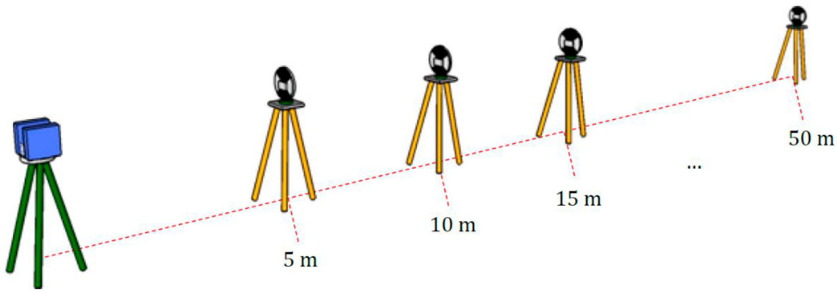
Figure 2.
Principles of object capturing with s-TLS (green) using identical points as signalized targets (yellow).
Figure 2.
Principles of object capturing with s-TLS (green) using identical points as signalized targets (yellow).
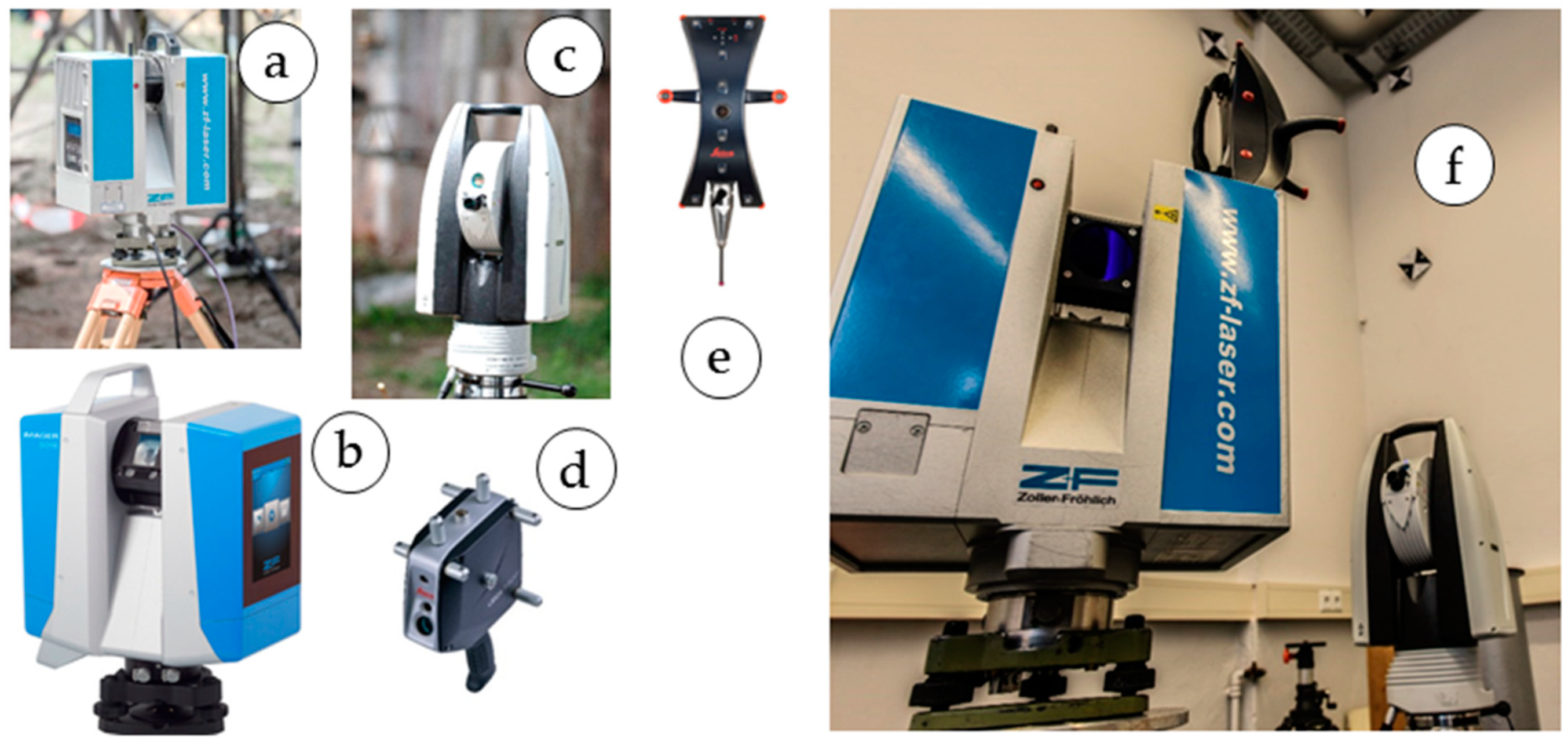
Figure 3.
Target mount for the combined adaption of the targets and corner cube reflectors (CCRs) (
a) target front, target mount with CCR, target back; (
b) CCR, target mount with target, target back [
22].
Figure 3.
Target mount for the combined adaption of the targets and corner cube reflectors (CCRs) (
a) target front, target mount with CCR, target back; (
b) CCR, target mount with target, target back [
22].
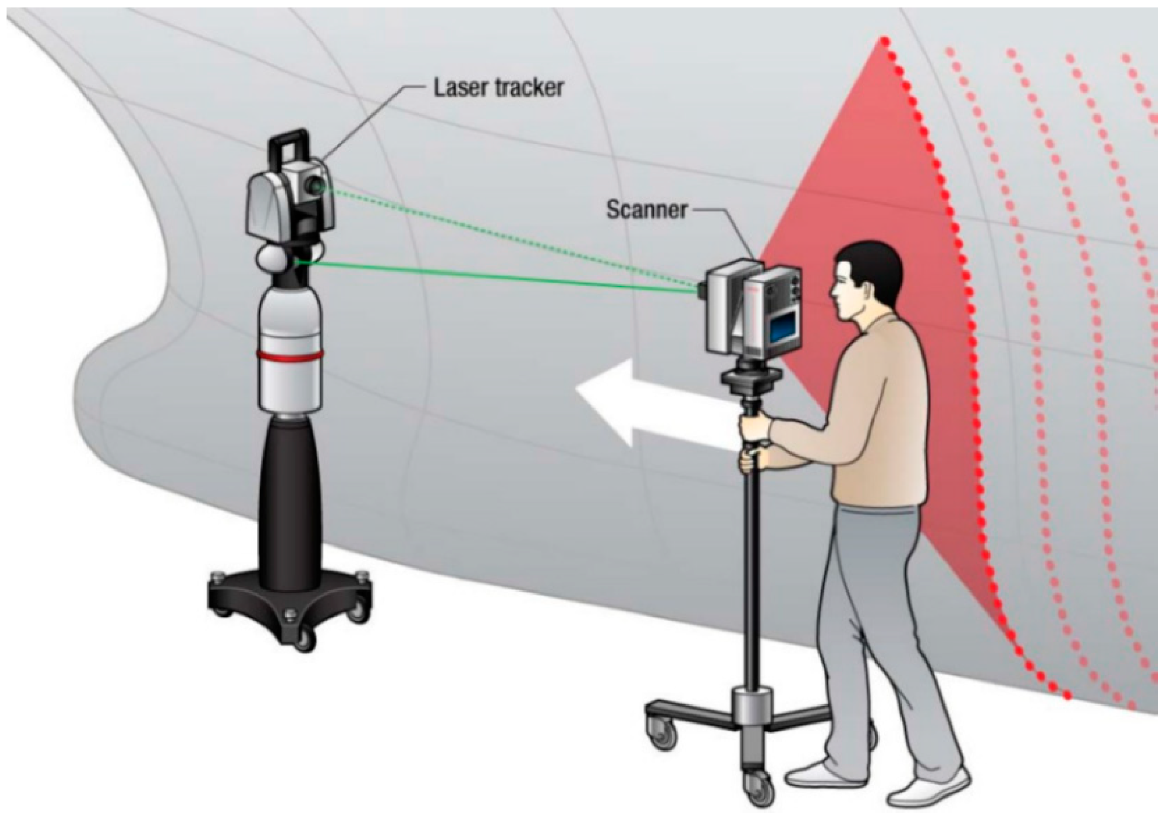
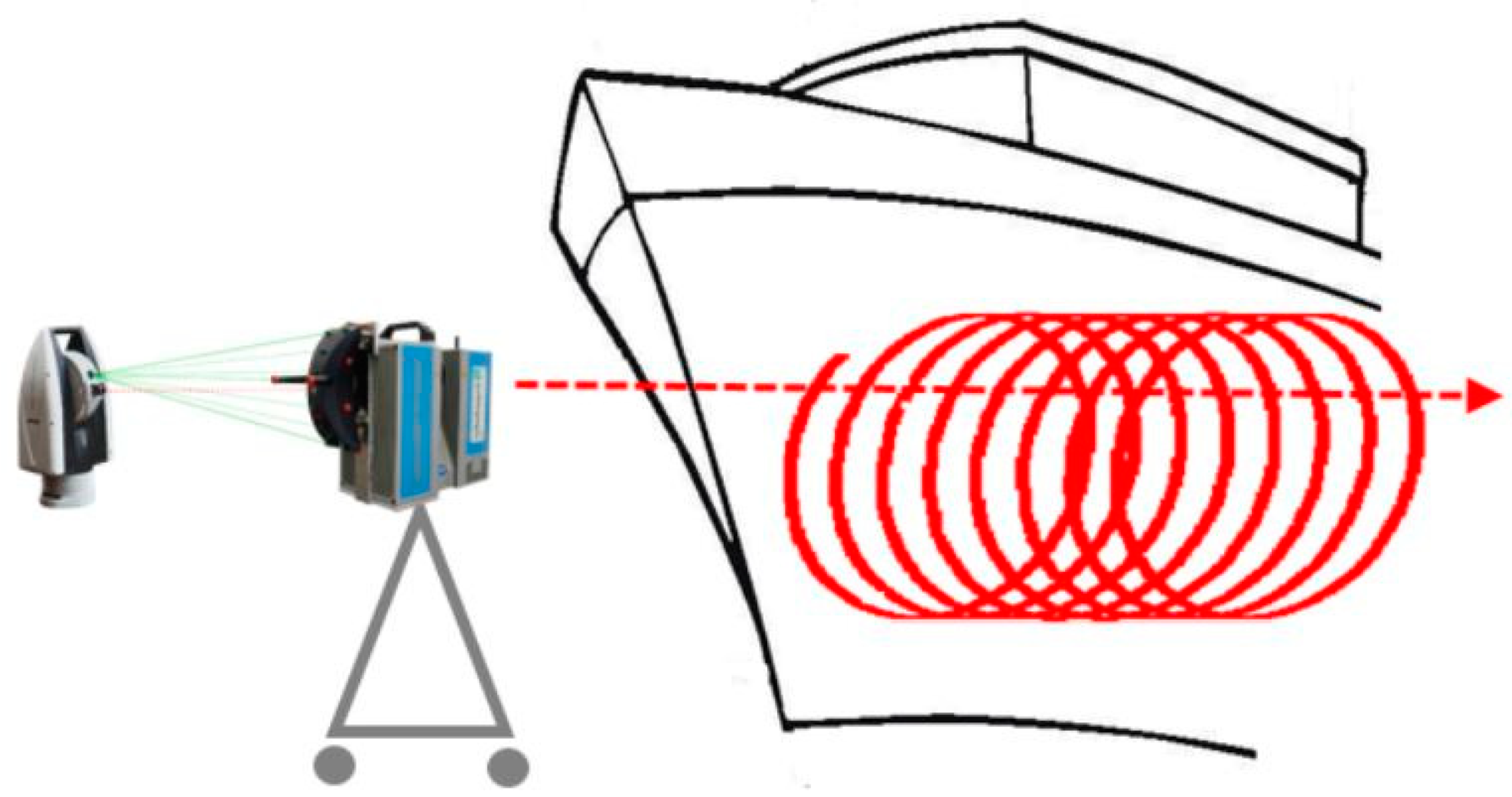
Figure 4.
Functional principle of the k-TLS-based MSS during object capturing [
30].
Figure 4.
Functional principle of the k-TLS-based MSS during object capturing [
30].
Figure 5.
Measuring of the reference points mounted on T-Probe with the Leica AT960 LR (10 measured LEDs in green, measured distance to reflector in red).
Figure 5.
Measuring of the reference points mounted on T-Probe with the Leica AT960 LR (10 measured LEDs in green, measured distance to reflector in red).
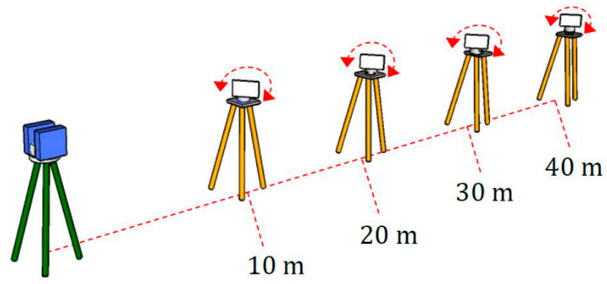
Figure 6.
Point by point (geo-) referencing of a k-TLS.
Figure 6.
Point by point (geo-) referencing of a k-TLS.
Figure 7.
Overview of the sensors used for the k-TLS-based MSS with their coordinate systems. The 6 DoF are assumed to be constant for the measurement period. The results from test measurements on reference geometries measured with a Leica T-Scan show that the 3D object capturing by k-TLS with a standard deviation of 1–2 mm is possible [
22,
31,
34] (distance to object approximately 5–10 m).
Figure 8.
Calibration set-up investigating distance- and target-dependent reflectivity with varying target grey values [
38].
Figure 8.
Calibration set-up investigating distance- and target-dependent reflectivity with varying target grey values [
38].
Figure 9.
Calibration set-up investigating distance and angle of incidence [
38].
Figure 9.
Calibration set-up investigating distance and angle of incidence [
38].
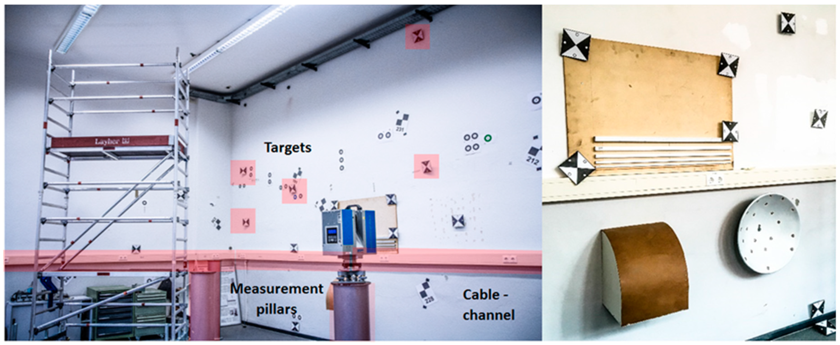
Figure 10.
The 3D-laboratory of the GIH with measurement pillars and cable channel (
left) and reference geometries (
right) [
22].
Figure 10.
The 3D-laboratory of the GIH with measurement pillars and cable channel (
left) and reference geometries (
right) [
22].
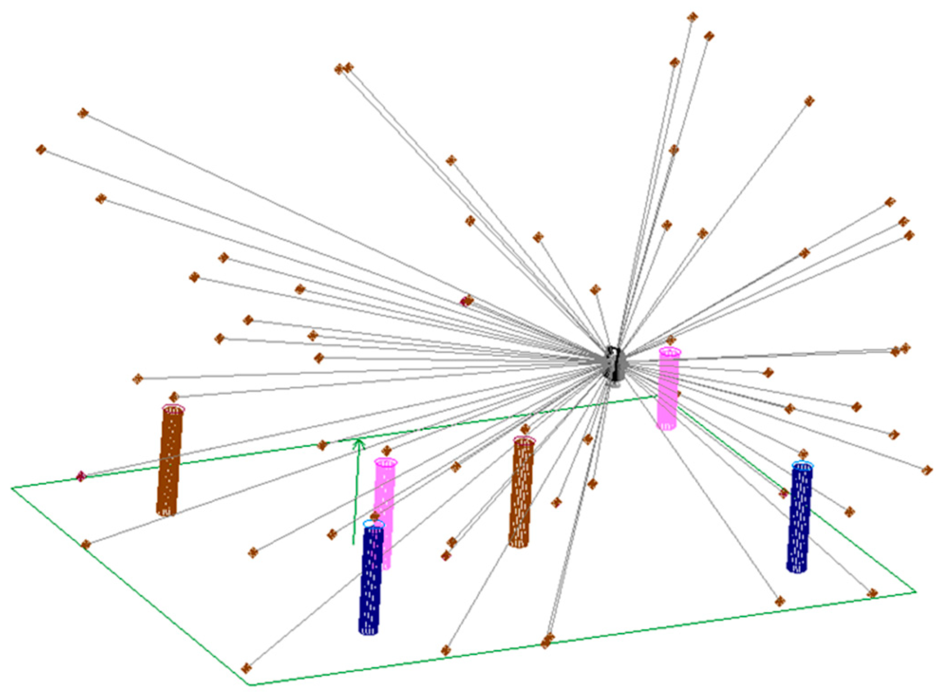
Figure 11.
Mock-up with reference points signalized by checkerboard targets (
Figure 3), origin of the reference frame. Moving direction of k-TLS and investigated (
Section 5) cylindrical geometry marked with red frame.
Figure 11.
Mock-up with reference points signalized by checkerboard targets (
Figure 3), origin of the reference frame. Moving direction of k-TLS and investigated (
Section 5) cylindrical geometry marked with red frame.
Figure 12.
Platform for k-TLS consisting of Z + F Imager 5010X working in 2D profiler mode, mounted on a dolly, (geo-) referenced by Leica AT960 and Leica T-Probe. The moving direction is marked by the red arrow. Movement and profiler mode are resulting in the shown scan helix.
Figure 12.
Platform for k-TLS consisting of Z + F Imager 5010X working in 2D profiler mode, mounted on a dolly, (geo-) referenced by Leica AT960 and Leica T-Probe. The moving direction is marked by the red arrow. Movement and profiler mode are resulting in the shown scan helix.
Figure 13.
Platform for k-TLS consisting of a Z + F Imager 5010X working in profiler mode, mounted on a rope-slide, (geo-) referenced by Leica AT960 and Leica T-Probe. The moving direction is marked by the red arrow. Movement and profiler mode are resulting in the shown scan helix.
Figure 13.
Platform for k-TLS consisting of a Z + F Imager 5010X working in profiler mode, mounted on a rope-slide, (geo-) referenced by Leica AT960 and Leica T-Probe. The moving direction is marked by the red arrow. Movement and profiler mode are resulting in the shown scan helix.
Figure 14.
Measurement and adjustment of the 56 reference points at the 3D-measurement laboratory of the GIH [
22].
Figure 14.
Measurement and adjustment of the 56 reference points at the 3D-measurement laboratory of the GIH [
22].
Figure 15.
Measurement of the reference geometries at the 3D laboratory of the GIH using T-Scan and laser tracker (
a) and k-TLS with laser scanner, laser tracker and T-Probe (
b) [
22].
Figure 15.
Measurement of the reference geometries at the 3D laboratory of the GIH using T-Scan and laser tracker (
a) and k-TLS with laser scanner, laser tracker and T-Probe (
b) [
22].
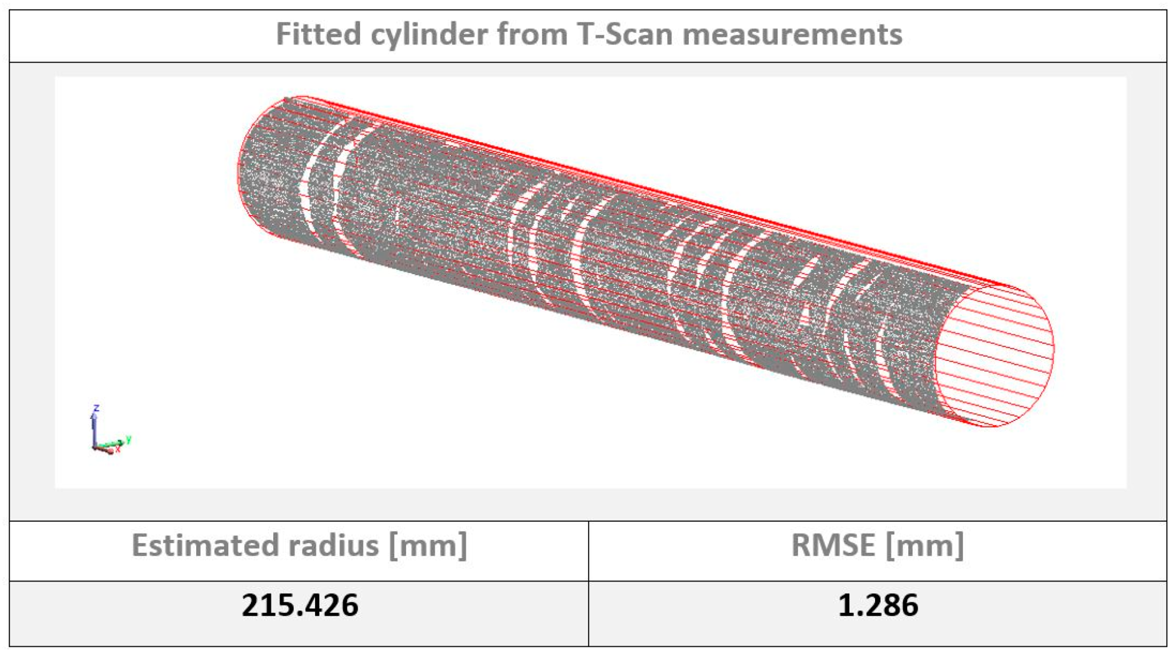
Figure 16.
Estimated cylinder from the 3D point cloud acquired by the T-Scan using the software SA.
Figure 16.
Estimated cylinder from the 3D point cloud acquired by the T-Scan using the software SA.
Figure 17.
Estimated cylinder from 3D point clouds acquired by s-TLS using the software Spatial Analyzer compared to estimated cylinder from the 3D point cloud acquired by the T-Scan (radius) and object-to-object relations (cylinder to cylinder/mutual perpendicular distance and angle between).
Figure 17.
Estimated cylinder from 3D point clouds acquired by s-TLS using the software Spatial Analyzer compared to estimated cylinder from the 3D point cloud acquired by the T-Scan (radius) and object-to-object relations (cylinder to cylinder/mutual perpendicular distance and angle between).
Figure 18.
Estimated cylinder from the 3D point cloud acquired by k-TLS with dolly using the software Spatial Analyzer compared to estimated cylinder from the 3D point cloud acquired by the T-Scan (radius) and object-to-object relations (cylinder to cylinder/mutual perpendicular distance and angle between).
Figure 19.
Estimated cylinder from the 3D point cloud acquired by k-TLS with rope-slide using the software Spatial Analyzer compared to estimated cylinder from the 3D point cloud acquired by the T-Scan (radius) and object-to-object relations (cylinder to cylinder/mutual perpendicular distance and angle between).
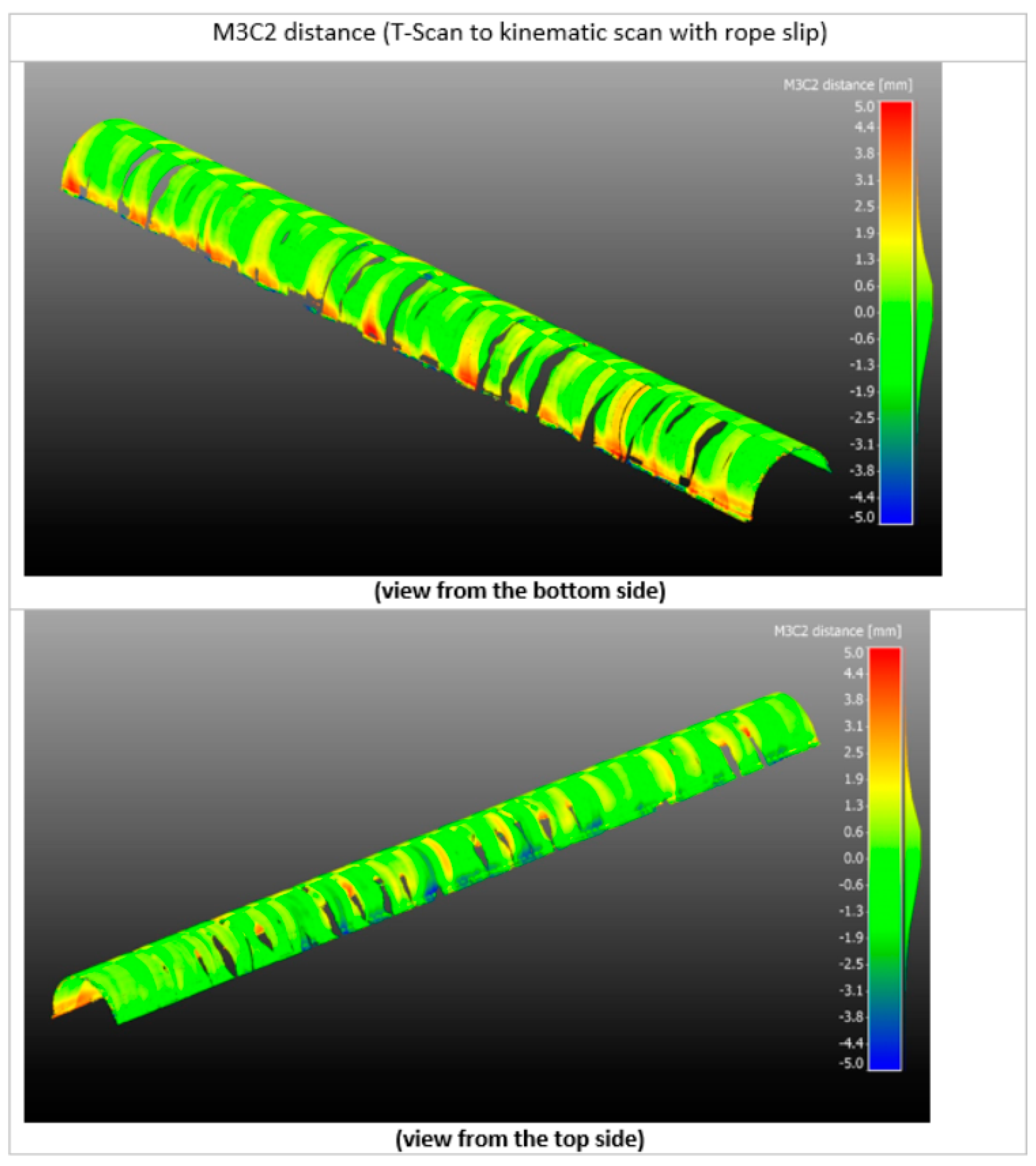
Figure 20.
M3C2 distances of two 3D point clouds (reference point cloud and k-TLS carried by dolly) showing the cylindrical part (top left: view from the bottom, bottom left: view from the top) of the mock-up (
Figure 11).
Figure 20.
M3C2 distances of two 3D point clouds (reference point cloud and k-TLS carried by dolly) showing the cylindrical part (top left: view from the bottom, bottom left: view from the top) of the mock-up (
Figure 11).
Figure 21.
Histogram of M3C2 distances for the comparison of the 3D point clouds acquired by the T-Scan and the k-TLS-based MSS using the dolly.
Figure 21.
Histogram of M3C2 distances for the comparison of the 3D point clouds acquired by the T-Scan and the k-TLS-based MSS using the dolly.
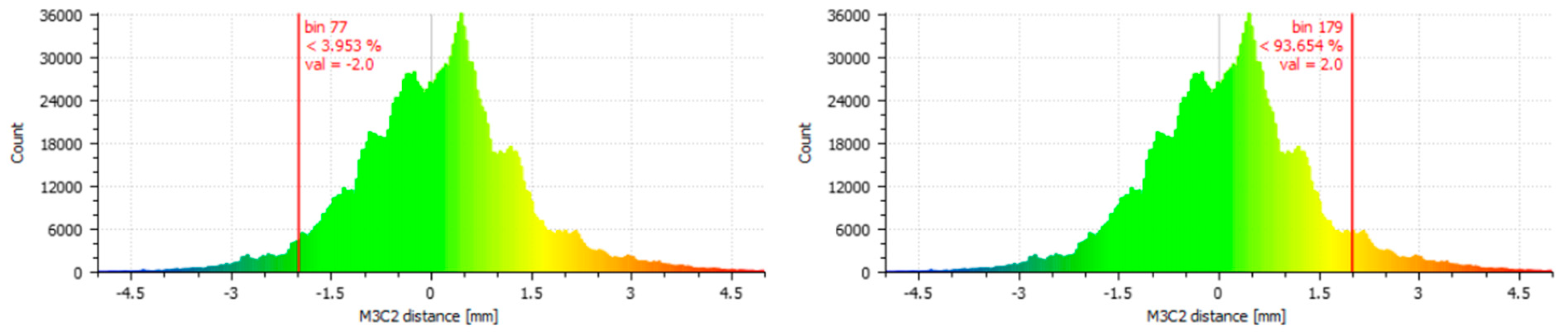
Figure 22.
M3C2 distances of two 3D point clouds (reference point cloud and k-TLS carried by rope-slide) showing the cylindrical part (top left: view from the bottom, bottom left: view from the top) of the mock-up (
Figure 11).
Figure 22.
M3C2 distances of two 3D point clouds (reference point cloud and k-TLS carried by rope-slide) showing the cylindrical part (top left: view from the bottom, bottom left: view from the top) of the mock-up (
Figure 11).
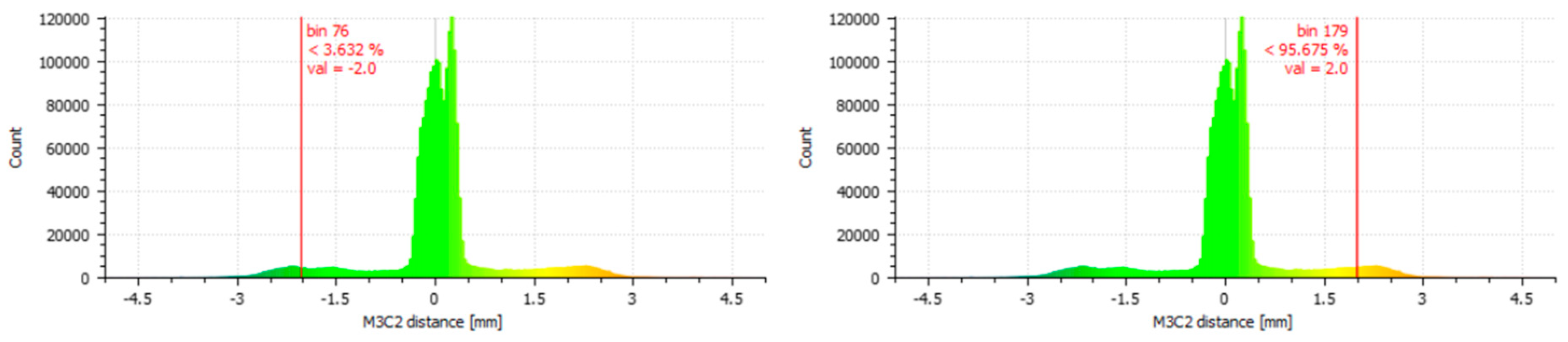
Figure 23.
Histogram of M3C2 distances for the comparison of the 3D point clouds acquired by the T-Scan and the k-TLS-based MSS using the rope-slide.
Figure 23.
Histogram of M3C2 distances for the comparison of the 3D point clouds acquired by the T-Scan and the k-TLS-based MSS using the rope-slide.
Figure 24.
M3C2 distances of two 3D point clouds (reference point cloud and s-TLS) showing the cylindrical part (top left: view from the bottom, bottom left: view from the top) of the mock-up (
Figure 11).
Figure 24.
M3C2 distances of two 3D point clouds (reference point cloud and s-TLS) showing the cylindrical part (top left: view from the bottom, bottom left: view from the top) of the mock-up (
Figure 11).
Figure 25.
Histogram of M3C2 distances for the comparison of the 3D point clouds acquired by the T-Scan and by the s-TLS.
Figure 25.
Histogram of M3C2 distances for the comparison of the 3D point clouds acquired by the T-Scan and by the s-TLS.
Figure 26.
Frontal view of the mock-up showing the M3C2 distances of the 3D point clouds captured with the T-Scan and k-TLS (dolly). The legend on the right side shows the histogram and the magnitude of the M3C2 differences. Profiles with lower accuracy, resulting from joints on the floor, are marked with red arrow.
Figure 27.
Bottom view on the mock-up showing the M3C2 distances of the 3D point clouds captured with the T-Scan and k-TLS (dolly).
Figure 27.
Bottom view on the mock-up showing the M3C2 distances of the 3D point clouds captured with the T-Scan and k-TLS (dolly).
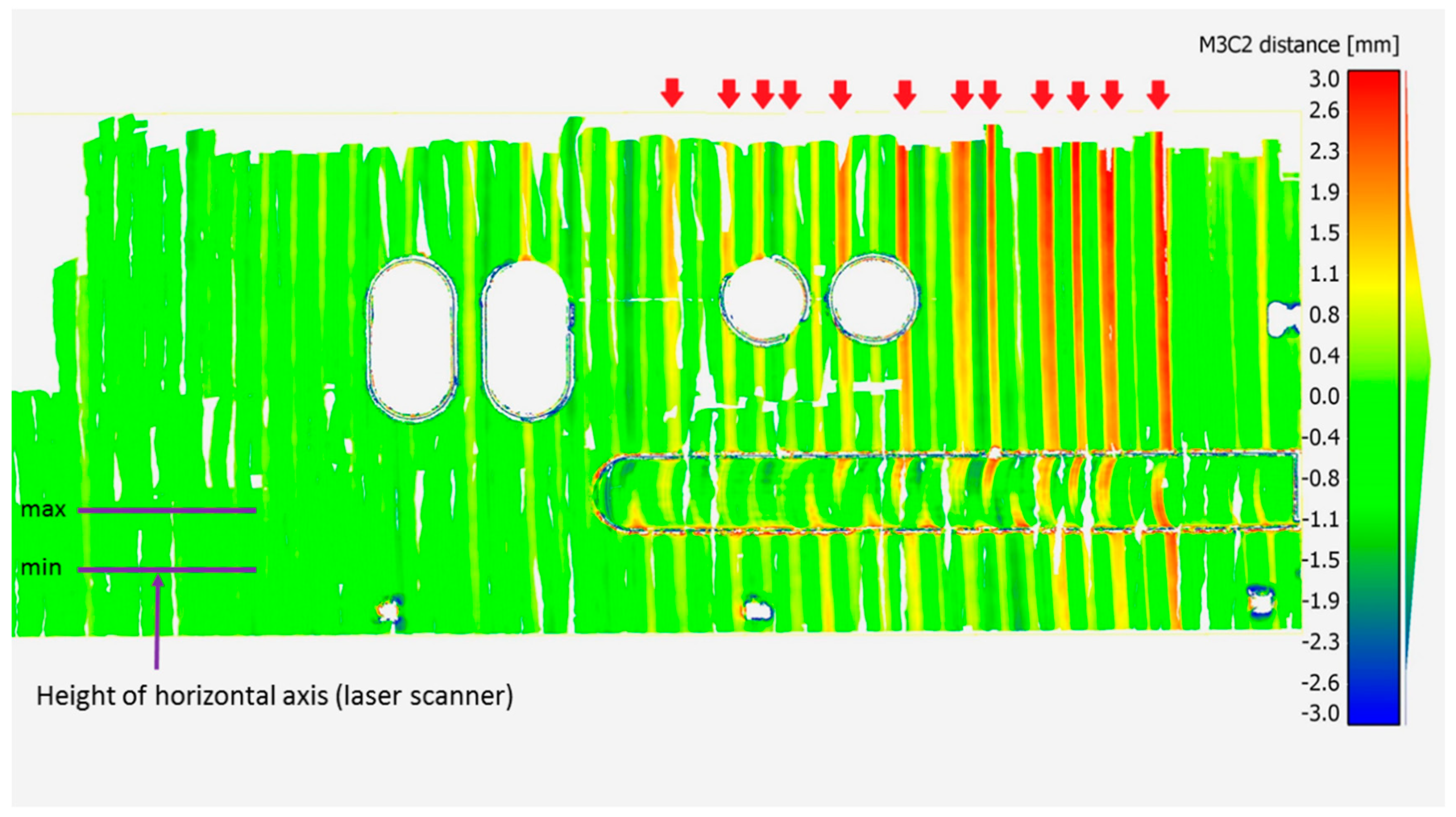
Figure 28.
Frontal view on the mock-up showing the M3C2 distances of the 3D point clouds captured with the T-Scan and k-TLS (rope-slide). The legend on the right side shows the histogram and the magnitude of the M3C2 differences. Differences resulting from pendulum movement of the laser scanner are marked by red arrows.
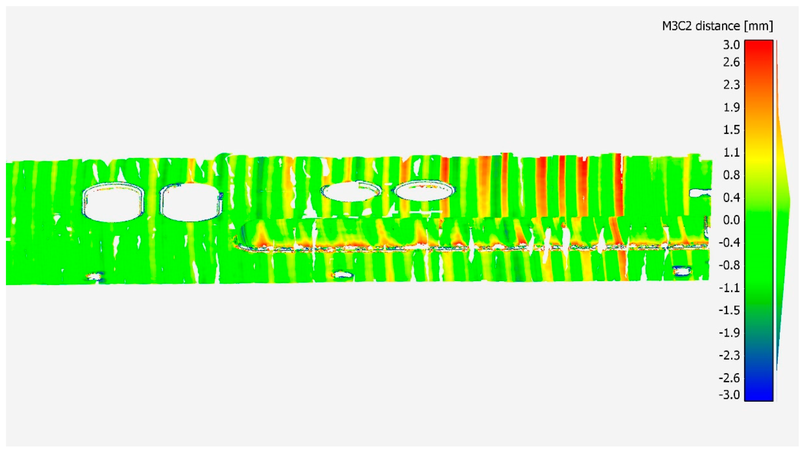
Figure 29.
Bottom view on the mock-up showing the M3C2 distances of the 3D point clouds captured with the T-Scan and k-TLS (rope-slide).
Figure 29.
Bottom view on the mock-up showing the M3C2 distances of the 3D point clouds captured with the T-Scan and k-TLS (rope-slide).
Figure 30.
Frontal view on the mock-up showing the M3C2-distances of the 3D point clouds generated with the T-Scan and s-TLS.
Figure 30.
Frontal view on the mock-up showing the M3C2-distances of the 3D point clouds generated with the T-Scan and s-TLS.
Figure 31.
M3C2 distances of the 3D point clouds captured by the T-Scan and s-TLS showing a bottom view of the cylindrical structure.
Figure 31.
M3C2 distances of the 3D point clouds captured by the T-Scan and s-TLS showing a bottom view of the cylindrical structure.
Figure 32.
Histogram of M3C2 distances [mm] for the entire mock-up (top-left and -right: T-Scan to k-TLS with dolly; middle-left and -right: T-Scan to k-TLS with rope-slide; bottom-left and -right: T-Scan to s-TLS.
Figure 32.
Histogram of M3C2 distances [mm] for the entire mock-up (top-left and -right: T-Scan to k-TLS with dolly; middle-left and -right: T-Scan to k-TLS with rope-slide; bottom-left and -right: T-Scan to s-TLS.
Figure 33.
The 3D point error in [mm] derived from the intensity values of the 3D point cloud captured by k-TLS at the mock-up (sensor platform: dolly, trajectory: 45° in relation to the mock-up, distance: ~3 m at the right, ~5 m at the left).
Figure 33.
The 3D point error in [mm] derived from the intensity values of the 3D point cloud captured by k-TLS at the mock-up (sensor platform: dolly, trajectory: 45° in relation to the mock-up, distance: ~3 m at the right, ~5 m at the left).
Figure 34.
3D point error in [mm] derived from the intensity values of the 3D point clouds captured by k-TLS at the mock-up (sensor platform: rope-slide).
Figure 34.
3D point error in [mm] derived from the intensity values of the 3D point clouds captured by k-TLS at the mock-up (sensor platform: rope-slide).
Figure 35.
The 3D point error in [mm] derived from the intensity values of the 3D point cloud captured by s-TLS at the mock-up (distance: ~5 m).
Figure 35.
The 3D point error in [mm] derived from the intensity values of the 3D point cloud captured by s-TLS at the mock-up (distance: ~5 m).
Table 1.
Accuracy of sensors used for providing the reference data [
24,
39].
Table 1.
Accuracy of sensors used for providing the reference data [
24,
39].
| Sensor | Accuracy |
|---|
| Leica AT960 LR | Ux,y,z = ±15 µm + 6 µm/m (3D accuracy, MPE) |
| Leica T-Scan 5 | Ux,y,z = ±60 µm under 8.5 m (MPE) |
| UP = ±80 μm + 3 μm/m (2 σ, uncertainty for plane surfaces, which is defined as the value of all deviations from the best-fit plane that is calculated with all measured points) |
Table 2.
Accuracy and standard deviations [
24].
Table 2.
Accuracy and standard deviations [
24].
| Parameter | Maximum Permissible Error (MPE) | Used Standard Deviation
|
|---|
| translations | | |
| rotations | | |
Table 3.
Uncertainties resulting of a total delay of 0.75 µs with respect to the mean velocities of the used platforms.
Table 3.
Uncertainties resulting of a total delay of 0.75 µs with respect to the mean velocities of the used platforms.
| Platform | Mean Velocity [m/s] | Uncertainty [µm] |
|---|
| dolly | 0.127 | 10 |
| rope-slide | 0.685 | 51 |
Table 4.
Parameters for s-TLS measurements at the industrial environment from (datasheet Z + F IMAGER 5010).
Table 4.
Parameters for s-TLS measurements at the industrial environment from (datasheet Z + F IMAGER 5010).
| Laser Scanner | Resolution | Quality |
|---|
| Z + F IMAGER 5010C | high | normal |
| 10,000 Pixel/360 deg | 25 rps/273 kHz |
Table 5.
Parameters of the k-TLS measurements with dolly and slip-line.
Table 5.
Parameters of the k-TLS measurements with dolly and slip-line.
| Platform | Frequency [Hz] | Number of Profiles | Points per Profile |
|---|
| dolly | 50 | 2791 | 20,000 |
| rope-slide | 50 | 1028 | 20,000 |
Table 6.
Results of the cylinder comparison with cylinder estimated from T-Scan 3D point cloud as reference data.
Table 6.
Results of the cylinder comparison with cylinder estimated from T-Scan 3D point cloud as reference data.
| Configuration | RMSE [mm] | Estimated Radius [mm] | Difference Radius T-Scan—TLS [mm] | Mutual Perpendicular Distance [mm] | Angle between [°] |
|---|
| T-Scan | 1.29 | 215.43 | --- | --- | --- |
| s-TLS | 1.42 | 214.80 | 0.62 | 0.3 | 179.98 (−0.02) |
| k-TLS dolly | 1.44 | 214.94 | 0.49 | 1.2 | 179.98 (−0.02) |
| k-TLS rope-slide | 1.58 | 214.72 | 0.70 | 0.01 | 0.73 |
Table 7.
Exemplary assessment of the (total) uncertainty of the s-TLS.
Table 7.
Exemplary assessment of the (total) uncertainty of the s-TLS.
| Platform | [m] | [mm] | [mm] | [mm] | [mm] |
|---|
| s-TLS (min) | 5 | 0.1 | 0.3 | 0.9 | 0.95 |
| s-TLS (max) | 6 | 1.3 | 1.34 |
Table 8.
Exemplary assessment of the (total) uncertainty of the k-TLS.
Table 8.
Exemplary assessment of the (total) uncertainty of the k-TLS.
| Platform | [m] | [m] | [mm] | [mm] | [mm] | [mm] | [mm] | [mm] |
|---|
| | | |
|---|
| dolly (min) | 2 | 3 | 0.1 | 0.16 | 0.011 | 0.10 | 0.1 | 0.15 | 0.5 | 0.59 |
| dolly (max) | 8.5 | 5 | 0.033 | 0.42 | 0.25 | 0.9 | 1.06 |
| rope-slide (min) | 5.5 | 4 | 0.024 | 0.27 | 0.20 | 0.8 | 0.90 |
| rope-slide (max) | 10 | 6 | 0.038 | 0.49 | 0.30 | 1.2 | 1.36 |


