Article

Comparing the Assimilation of SMOS Brightness Temperatures and Soil Moisture Products on Hydrological Simulation in the Canadian Land Surface Scheme

1
Department of Geography, Environment & Geomatics, University of Guelph, Guelph, ON N1G 2W1, Canada
2
Climate Research Division, Environment and Climate Change Canada, Toronto, ON M3H 5T4, Canada
3
Environment and Climate Change Canada, Saskatoon, SK S7N 3H5, Canada
*
Author to whom correspondence should be addressed.
Remote Sens. 2020, 12(20), 3405; https://doi.org/10.3390/rs12203405
Submission received: 8 September 2020 / Revised: 10 October 2020 / Accepted: 12 October 2020 / Published: 16 October 2020
(This article belongs to the Special Issue Satellite Hydrological Data Products and Their Applications)

Abstract

:
Soil moisture is a key variable used to describe water and energy exchanges at the land surface/atmosphere interface. Therefore, there is widespread interest in the use of soil moisture retrievals from passive microwave satellites. In the assimilation of satellite soil moisture data into land surface models, two approaches are commonly used. In the first approach brightness temperature (TB) data are assimilated, while in the second approach retrieved soil moisture (SM) data from the satellite are assimilated. However, there is not a significant body of literature comparing the differences between these two approaches, and it is not known whether there is any advantage in using a particular approach over the other. In this study, TB and SM L2 retrieval products from the Soil Moisture and Ocean Salinity (SMOS) satellite are assimilated into the Canadian Land Surface Scheme (CLASS), for improved soil moisture estimation over an agricultural region in Saskatchewan. CLASS is the land surface component of the Canadian Earth System Model (CESM), and the Canadian Seasonal and Interannual Prediction System (CanSIPS). Our results indicated that assimilating the SMOS products improved the soil moisture simulation skill of the CLASS. Near surface soil moisture assimilation also resulted in improved forecasts of root zone soil moisture (RZSM) values. Although both techniques resulted in improved forecasts of RZSM, assimilation of TB resulted in the superior estimates.

Graphical Abstract

1. Introduction

Soil moisture (SM) is one of the most important variables affecting the land surface water and energy budgets. It is one of the major components that impacts the terrestrial water, energy and biogeochemical cycles by constraining the evapotranspiration from land [1,2,3]. It is involved in a series of feedback processes at different scales from local to global and is one of the key initial condition variables for climate and weather prediction models [4]. It also impacts the ground water recharge and river outflow by controlling the division of rainfall into infiltration, percolation and runoff in a basin [5,6]. Soil moisture has further impacts on air temperature and atmospheric stability by constraining the partition of the incoming solar radiation into latent and sensible heat fluxes [2,7]. The occurrence of high temperature extremes and heat waves are also related to SM deficits [8,9]. Soil moisture also influences land carbon uptake by governing the water stress for vegetation [10]. Accurate spatial and temporal estimation of SM is essential in many fields such as agriculture, ecology, water resource management, flood and drought forecasting as well as predicting the impacts of future climate change [11,12].
The conventional methods to obtain SM data are ground-based in situ measurements, simulation of SM by land surface models forced by meteorological observations, vegetation and soil parameters and remote sensing [13,14]. At the local scale in situ networks provide ground truth data but it is not feasible to have in situ networks deployed at large scale as SM varies in both space and time. Estimating SM by running a land surface model on a large spatial scale also comes with limitations in the form of inaccurate initial conditions, and a lack of high quality meteorological forcing observations on a global scale, inaccurate model physics, incomplete observations in space and time and errors in parameter estimations [5,14,15,16]. Therefore, satellite remote sensing provides a useful platform to map the SM and other variables globally and over long periods of time and at regular intervals [17,18,19]. Another advantage of satellite remote sensing is that these systems are capable of measuring the SM in all weather conditions at diurnal frequencies, provided it is operated at a frequency transparent to vegetation, atmosphere and clouds [20]. Passive microwave sensors operating at low frequencies can provide large scale SM estimates suitable for regional and global applications. The Soil Moisture and Ocean Salinity (SMOS) satellite, launched in 2009 by the European Space Agency (ESA), operates in passive L-Band microwave, the satellite mission was dedicated to global surface moisture monitoring over land and sea surface salinity over oceans. SMOS also provides significant information on vegetation moisture content and root zone soil water content [21]. The Soil Moisture Active Passive (SMAP) satellite, launched in 2015 by the National Aeronautics and Space Administration (NASA), also operating in passive L-Band microwave, monitors surface SM [3]. Both SMOS and SMAP missions also address many scientific problems in hydrometeorology including and not limited to flood forecasting, drought monitoring and numerical weather prediction [22].
Satellite microwave remote sensing data alone are not adequate due to the coverage breaks in space and time and also they can directly measure only the surface SM [13]. Remotely sensed SM estimations from microwave satellites often have coarser spatial resolutions compared to land surface models [23]. Therefore in order to estimate the best SM conditions we have to optimally combine, the satellite data, data from in situ monitoring networks and land surface model output in a process called data assimilation [4,24,25]. Data assimilation gives the best estimate of the state of the system from incomplete and inaccurate dynamical models and erroneous observations [26]. There are many data assimilation systems incorporated into numerical weather forecasting systems that assimilate the passive microwave brightness temperature data into the land surface models to get a better estimate of the SM state such as the European Centre for Medium-Range Weather Forecasts (ECMWF) Numerical Weather Prediction (NWP) [4,27,28], National Centers for Environmental Prediction (NCEP) Global Forecast System (GFS) [29] and the Canadian Land Data Assimilation System (CaLDAS) [30]. This improved estimate of the SM will provide the requisite conditions for improving the predictions of water and energy balance of the surface [31,32,33].
A number of studies have investigated the assimilation of satellite SM data into land surface models [14,30,34,35,36,37,38]. In studies examining the impact of assimilation of passive microwave derived estimates of SM into land surface models, two approaches are commonly used. In the first approach, brightness temperature (TB) data are assimilated into the land surface model using a radiative transfer model (RTM) such as Community Microwave Emission Model (CMEM) [30,39,40,41] while in the second approach, SM products derived from the passive microwave TB are assimilated [5,35,42]. For example, Xu at al. [42] assimilated the SMOS retrieved SM product into the Modélisation Environmentale Communautaire-Surface and Hydrology (MESH) model over the Great Lakes basin using a one-dimensional Ensemble Kalman Filter (EnKF). Their study showed the skill of SMOS in measuring the SM in a wide range of vegetation covers. The study also showed that the skill of the assimilated product is better than the SMOS observation and the open-loop skill of the model alone. Similarly, Zhao et al. [43] showed that assimilating the SMOS level 2 (L2) product into a land surface model over the central Tibetan Plateau resulted in an estimate superior to the cases where open-loop land surface modeling or remote sensing derived SM alone is used. Ridler et al. [5] found that assimilating SMOS retrieved SM product in a fully integrated hydrological and soil–vegetation–atmosphere transfer model in Western Denmark improved the SM correlations in the surface layer and root zone at 25 cm. One of the potential disadvantages of assimilating the retrieved SM product over the TB is the unknown errors arising from the inversion algorithm used for retrieving the SM from the TB. The errors in the input variables and discontinuity in the derivative of order zero or higher in the inversion algorithm can lead to a poor solution [44]. In the case of direct TB assimilation, an RTM or backscatter model is coupled with the land surface model. The RTM works as a forward modeling platform, which translates the land surface model simulated SM into observed variable brightness temperature. The data assimilation term for the model that maps the model state variables from the model space to the observation space is known as observation operator [36,45,46]. Atmospheric RTMs play an important role in the satellite data assimilation for NWP application as satellites measure radiances and do not observe directly the geophysical variables such as humidity, temperature or cloud properties [47]. De Lannoy and Reichle, 2016 [38] assimilated both the SMOS TB and SM retrievals into the Goddard Earth Observing System Model, version 5 (GEOS-5). They found similar domain-average skill matrices for both the assimilation experiments but varying skill levels locally. Recently, another approach has been also investigated assimilating the Neural Network (NN)-based SM retrievals [48,49,50]. In this approach, the NN is trained using the observed TB from the satellite as input and the simulated SM data from land surface model as reference for the training. One of the advantages of this method is that there is no need to do further bias correction. This NN approach has been used for both the SMOS [50] as well as SMAP [48,49] TB data assimilation.
Since the advent of microwave remote sensing, the assimilation and validation of SM data, retrieved or raw TB is an active area of research. However, there is not a significant body of literature comparing the differences between these two approaches. Further, there are not many studies on assimilating SM into the Canadian Land Surface Scheme (CLASS) model, the land surface component of the Canadian Seasonal and Interannual Prediction System (CanSIPS) of Environment and Climate change Canada (ECCC).
In this paper, we present our investigation into (i) the difference between assimilating the SMOS TB vs the SMOS SM retrieval into the CLASS and if there is any particular advantage by using one method over the other, (ii) how the assimilation of top layer SM affects the SM estimation at the root zone, which has significant impacts on evapotranspiration rate especially in vegetated regions. This paper is organized as follows. Section 2.1 describes the models used in this study. Section 2.2 introduces the SMOS data, the study site and in situ data. In Section 2.3, there is a brief presentation about the EnKF. Section 2.4 describes the data assimilation experiment set-up. The results and discussion are presented in Section 3 and Section 4 respectively, and Section 5 holds the conclusion.

2. Models, Data, Methods and Experimental Set-Up

2.1. Models

2.1.1. The Canadian Land Surface Scheme (CLASS)

The land surface model used in this study was the Canadian Land Surface Scheme, CLASS, the land surface component of the Canadian Global Climate Model or GCM [51,52]. CLASS simulates energy and water balance of the land surface forward in time from an initial condition forced by atmospheric data. CLASS can be run in offline mode or can be coupled with an atmospheric model. The prognostic variables that must be initialized at the beginning of the CLASS simulation include the frozen and liquid water content and the temperature of each of the soil layers; mass, temperature, density and albedo of the snow pack if present; the temperature and amount of intercepted rain and snow on the vegetation canopy; the temperature and depth of ponded water on the soil surface; an empirical vegetation growth index [40]. We also needed to specify the soil and vegetation parameters of the area being simulated. The hydrological and thermal properties as well as the albedo of the soil vary according to the texture and moisture content of the soil [51,52].
In this study, we used version 3.6 of the CLASS standalone driver. The soil column was divided into three layers with bottom boundaries at 0.05, 0.20 and 4.10 m, respectively, from the soil surface. The top layer boundary was set to 0.05 m in order to be consistent with the depth of the SMOS satellite SM measurement. Verseghy [53] provide extensive details regarding CLASS components and model physics. Energy and moisture fluxes were calculated at the top and bottom of each of the three layers in CLASS. The prognostic variables, soil water content and temperature at each layer were advanced in time in accordance with the calculated energy and moisture fluxes. The moisture fluxes were modeled using the Green–Ampt theory in the case of infiltration, while Darcy’s method was used in the case of water transfer between the soil layers and drainage [54,55].
The atmospheric forcing data (Table 1) was required to run CLASS include incoming shortwave and longwave radiation, precipitation, air temperature, specific humidity, wind speed and atmospheric pressure [55]. The meteorological forcing data we used were from the North American Regional Reanalysis (NARR, [56]) data. We interpolated the three-hourly meteorological forcing data into 15 min intervals. CLASS is run at a time step of 15 min. The parameters used to run CLASS include maximum leaf area index, roughness length, above ground biomass density, rooting depth and minimum stomatal resistance. Values assigned to these parameters were chosen according to the observation and are summarized in Table 2 and Table 3.

2.1.2. Community Microwave Emission Model (CMEM)

The Community Microwave Emission Model (CMEM) [57,58] was developed by the ECMWF to simulate the low frequency passive microwave brightness temperatures (from 1 to 20 GHz) of the surface as seen by passive microwave sensors included on a number of earth observation satellites. We used CMEM version 5.1 in our study. Input to the CMEM include SM and temperatures of the different soil layers, surface temperature, leaf area index, vegetation and soil parameters. The parameters and models used in CMEM are summarized in Table 4. The CMEM model physics follows the parameterization based on the Land Surface Microwave Emission Model [59] and L-Band Microwave Emission of the Biosphere (L-MEB) [60]. The high modularity of CMEM allows for consideration of different parameterizations for soil dielectric constant, effective temperature, soil roughness, vegetation opacity and atmospheric contribution [61]. The vegetation opacity model of Wigneron at al. [60] was used in this study.
In the SMOS TB assimilation, CMEM was used as the observation operator or observation model, which maps the model state variables from the model space to the observation space [45,46]. One of the reason for using an observation operator is because satellite measurements, such as radiance or brightness temperature, is only indirectly related to the land surface variables of interest and observation operator facilitates the conversion of model simulated variables to the satellite observed variables [45]. Using the SM inputs simulated by CLASS, CMEM can predict a brightness temperature estimate that can be compared to satellite observed brightness temperature from the same wavelength.

2.2. Observation Data

2.2.1. SMOS

The Soil Moisture and Ocean Salinity (SMOS) satellite was launched by the ESA to collect global surface SM from approximately 0–5 cm depth of soil [21,66]. The Microwave Imaging Radiometer with Aperture Synthesis (MIRAS) onboard SMOS provides multi angular, bi-polarized brightness temperatures (TB) at L-band. It covers a spatial resolution of 43 km on average with a repeat cycle of less than three days. The target accuracy of the mission was ±0.04 m 3 ·m 3 [67]. For the direct TB assimilation we used the SMOS estimated brightness temperature (TB) (MIR-SCLF1C product version 620) at both horizontal (H) and vertical (V) polarization. For SM retrieval assimilation we used SMOS SM retrieval L2 product (MIR-SMUDP2 product version 620). Both the SMOS TB and L2 products are available to download from ESA website (https://smos-diss.eo.esa.int/oads/access/collection/SMOS_Open/tree). In our experiment, we used the SM retrieval data that falls within the realistic range of 0.02–0.6 m 3 ·m 3 . The brightness temperature observations were retained only when it falls with in the range of 100−320 K. The SM product was retrieved from the TB using the L-MEB forward algorithm [60], which is an iterative algorithm that matches the surface emission observed by SMOS to the modeled L-band emission of the surface [68,69]. We used the TB data at an angle of approximately 40°. The L2 SM was obtained by minimizing a cost function between the SMOS observed TB and the simulated L-MEB TB. The forward model requires the parameters such as SM, land surface temperature, land cover information, leaf area index and soil properties [5,67].

2.2.2. In Situ Data (Study Sites and Ground Data Measurements)

This study was applied over the Brightwater Creek watershed in Saskatchewan Canada (Figure 1) using in situ SM network run by the University of Guelph and Environment and Climate Change Canada. The distribution of sensors in the network was arranged over a 40 by 40 km study domain situated within an agricultural region [70]. The region is characterized by agricultural activities, with typical crops including wheat, chick peas and canola. The network was designed to capture SM variability within a footprint of a passive microwave radiometer and has been used previously for the validation of SMOS SM retrievals [71]. In situ SM measurements were recorded using a Stevens Hydra Probe II SDI-12 sensor. All soil moisture monitoring stations have a minimum of three Stevens Hydra Probe sensors horizontally installed into the soil profile at 5, 20 and 50 cm depths. The physical measurements obtained by these probes is described by [72] but, briefly, the probes use an impedance-based approach to characterize the dielectric properties of the soil using a radio frequency at 50 MHz. The reflected frequency was measured along four 5.7 cm tines extending from a 3.4 cm diameter sensor head [72]. Using previously established calibration equations [73], the measured real dielectric was converted to soil moisture. Stevens Hydra Probe SM sensors used in this study were calibrated using infiltration wet-up and dry-down laboratory calibration procedures by Burns et al. [73]. The calibration utilized the soil samples collected from the study site at Brightwater Creek watershed, in Saskatchewan Canada. The soil samples were collected from 5, 20 and 50 cm and of different textural compositions. The calibration experiments found that the RMSE values of the sensors were <0.019 m 3 ·m 3 , which are significantly less than the SMOS targeted accuracy of ±0.04 m 3 ·m 3 . More details about the senor calibration can be found in Burns et al. [73]. The network contains 36 stations and previous research by Rowlandson et al. [74] demonstrated that the mean of the network was appropriate for estimating the SM average within the passive microwave footprint. More details about the network can be seen in Tetlock et al. [70] and Burns et al. [75].

2.3. Assimilation Methods

2.3.1. Ensemble Kalman Filter (EnKF)

Advanced Kalman based filters have been widely used in geophysical data assimilation in recent years [76,77,78,79]. The Kalman filter [80] provides the best linear unbiased estimate of the system considering the past measurements and dynamics of the fluid system under consideration. The nonlinearity and large number of degrees of freedom limits the application of standard Kalman filter for numerical weather prediction and climate prediction models [78]. In the extended Kalman filter (EKF), standard Kalman filter equations are applied after linearizing the nonlinear models but the requirement of derivation of Jacobian or Tangent Linear Model (TLM) for the linearization of the nonlinear model is a computationally expensive process. EKF also neglects the contribution from higher order moments in calculating the error statistics [78,81,82]. The Ensemble Kalman filter (EnKF), introduced by Evensen [81], estimates the error statistics from ensembles integrated through the nonlinear models [83] and there is no need to linearize the nonlinear models.
The main concept behind the derivation of EnKF is based on forecasting the error statistics using Monte Carlo methods or ensemble integration. Thus, if the forecast model is interpreted as a stochastic differential equation, the forecast-error statistics can be approximated using ensemble integration [78,81]. For EnKF, there is no need for any closure approximation for calculating the error covariance, whereas in the Extended Kalman Filter (EKF), closure approximation is applied by neglecting contributions from higher-order statistical moments in the error covariance evolution equation. Therefore in EnKF, the error covariance matrices can be calculated by integrating the ensemble of model states in time via fully nonlinear model equations. Thus, all the statistical information such as mean and covariances about the predicted model state that is required at the time of analysis is obtained from the ensembles [81,82]. EnKF and its derivatives have been popular in atmospheric and oceanic data assimilation because of its algorithmic simplicity, flow dependent error structure, ease of implementation and comparatively lower computational cost [78].
Consider that X t is the state of a dynamical model at time ‘t’ and Y t is the observation at time ‘t’. The state space equations of the dynamical system can be expressed as
X t = f ( X t 1 , q t 1 )
Y t = h ( X t , r t )
where f( ) is the nonlinear function which takes state X t 1 to X t and q t 1 is the random model error following a Gaussian distribution with zero mean and covariance Q t 1 , h( ) is the observation or measurement function and r t is the observation noise, which is also Gaussian with mean zero and covariance R t .
In the EnKF, each ensemble member is propagated forward in time through the nonlinear model and corrected whenever new measurements are available [78] and the cycle is repeated. The state update equations are given by,
X t a = X t b + K t ( Y t H X t b )
K t = P t b H T ( H P t b H T + R ) 1
P t b = E [ ( X t b X t b ¯ ) ( X t b X t b ¯ ) T ]
P t a = ( I K t H ) P t b ( I K t H ) T + K t R K t T = ( I K t H ) P t b
where X t a is the analyzed state and H is the linearized observation operator. The subscript ‘b’ indicates the model forecast state, K t is the Kalman gain, P t b is the forecast error covariance, E [ . ] represents the statistical expectation value, the overbar denotes the ensemble mean and P t a is the analysis error covariance. I is an identity matrix.
In ensemble based filters such as EnKF, the ensemble members account for the uncertainties in initial conditions. A finite number of ensemble members reduces the accuracy of the estimate of the statistical moments, however a large number of ensemble members is computationally expensive [78,83]. Not accounting for the model errors because the model is not perfect and initial condition errors because of the limited number of ensemble members will leads to the underestimation of the background error-covariance matrix. This can be addressed by using a covariance inflation method [84,85,86]. The most common methods used are additive inflation [87] and multiplicative inflation [84]. In the multiplicative-inflation method, the raw background covariance matrix is multiplied by a small number greater than one. In our study we used an additive inflation method, in this method, an additional random term with some covariance structure is added to the background error covariance matrix [85,88,89].

2.3.2. Bias Correction

Generally there is a large systematic bias between the satellite derived and model derived SM products because of the uncertainties in RTMs, land surface and vegetation parameters, errors in the land surface models and inaccurate atmospheric forcing [58,90,91,92]. One commonly used method for addressing the bias is rescaling the satellite observations to long term model simulations. Data assimilation techniques based on Kalman filters assume unbiased observation and model forecast [46]. We applied a prior bias correction to the SMOS data based on the Cumulative Distribution Function (CDF) matching [90,92] before the assimilation. For SMOS SM retrieval bias correction, CDF matching was applied using the four years (2011–2014, April to September) of CLASS simulation data and SMOS SM retrieval data and SMOS SM retrieval was rescaled into CLASS climatology. For SMOS TB bias correction, we applied the CDF matching between the four years (2011–2014, April to September) of CMEM forward simulation data and SMOS observed TB data. The initial conditions for the CMEM forward simulations were provided by CLASS data. In our experiment, for CDF matching, we used the data only from April to September because CDF matching can work as an additional source of error by discarding the seasonal cycles in biases [91,92]. The standard deviation for the observation error for the SM retrieval was set as 0.04 m 3 ·m 3 according to the target accuracy of SMOS. The standard deviation of the observation operator for the SMOS TB was set as 5 K, this include the instrumental errors in radio meter and uncertainties in forward simulations using CMEM.

2.4. Experimental Set-Up
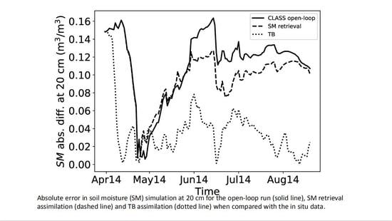
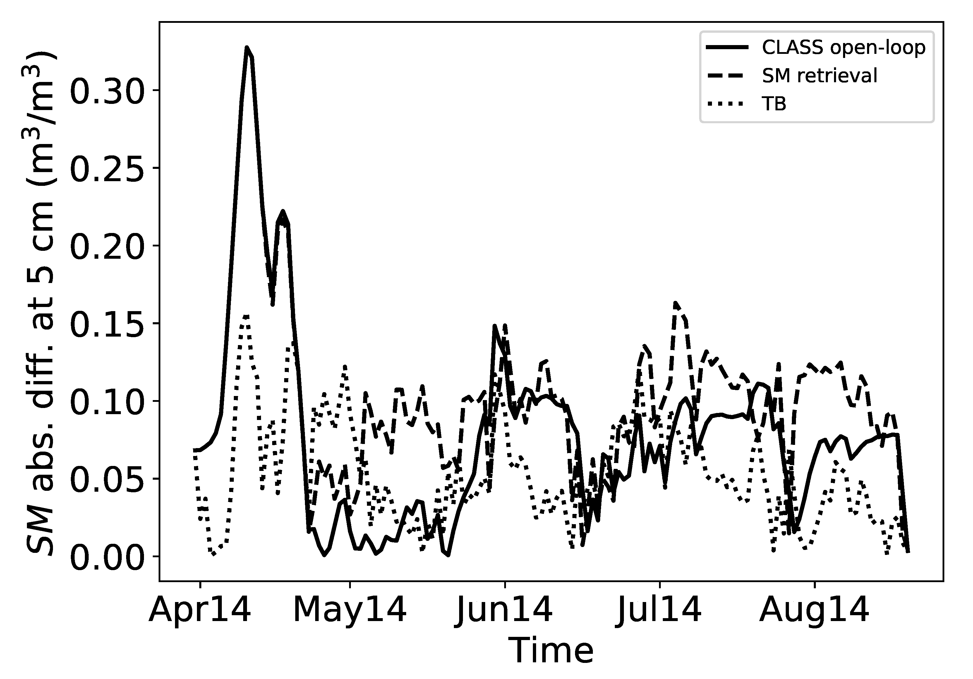
It is a challenge to find an optimal method that satisfies all the conditions over a large range of constraints including different land surface models, different data assimilation schemes and different land characteristics. This study was applied over an agricultural region in Saskatchewan, Canada. For the assimilation of TB, CLASS was coupled with CMEM. We employed the EnKF data assimilation scheme of Evensen [76].
Before starting the assimilation and open-loop integration, CLASS was spun-up by cycling the model continuously through the period April 2011 to March 2014 for the model states to be in equilibrium with the forcing meteorology. Please note that only the CLASS model was spun-up and not the entire data assimilation system. This spin-up process was independent from the CLASS simulations performed to build the CDFs (explained in Section 2.3.2). The initial conditions obtained from the CLASS spin-up process was used for the open-loop simulations and data assimilation. At first the CLASS open-loop run (no data assimilation) was performed in deterministic mode forced by the NARR atmospheric data for the period April 2014 to September 2014. Two different approaches of data assimilation experiments were conducted using the EnKF method. The first set of experiments SM retrieval (SM-L2 product) from the SMOS satellite was assimilated into the CLASS model; whereas the second set of experiment TB from SMOS was assimilated into the CLASS model using CMEM as the forward model. The estimation skill of both the approaches as well as the CLASS open-loop run experiment were compared with the in situ SM data.
In the first state estimation experiment, the retrieved SM (SM-L2 product) data from the SMOS was assimilated into the CLASS from April 2014 to September 2014 using the EnKF algorithm. The SM data was assimilated whenever it was available, the repeat cycle of SMOS was less than three days. In SM retrieval assimilation, the model simulated variable and observed variable were SM, therefore there was no need of an RTM and the observation operator was an identity matrix. The second approach was identical to the first approach except that we assimilated SMOS observed TB instead of SM retrieval. In this state estimation experiment, CLASS predicted SM was brought into the observation space with the use of an observation model. The observation model used in this study was the CMEM. The parameters used in CMEM are explained in Section 2. The schematic of the TB assimilation is given in Figure 2.
In EnKF, there are different perturbation strategies for initial ensemble generation, from the simple addition of pure random perturbation to the advanced singular vectors. Addition of purely random perturbation can lead to dynamical imbalance and deterioration of the quality of the ensembles [93]. We perturbed only the CLASS SM variable using Random Field (RF) perturbation technique [93] that results in flow balanced ensembles, and did not perturb the meteorological forcing variables. The initial ensembles were generated by adding the observed SM values from the in situ data with differences of randomly chosen SM states from historical run of CLASS for the period of April 2011 to April 2014, the differences were scaled to zero mean before the addition. In this study, an additive inflation method [85,88,89] was used to account for the model error. The mean of the perturbations were scaled to zero and standard deviation equal to the climatological (April 2011 to April 2014) standard deviation (0.065) of the CLASS simulated surface SM. We used a random subset of model predictions of SM fields from a historical run of CLASS and scaled them to zero mean and added one of these subsets into one of the background ensemble member following Li et al. [85].
The assimilation experiments were performed whenever the observation data were available for the period from April 2014 to September 2014. For the same period, a open-loop run of CLASS was also completed, forced by the NARR data. The background and observation errors were assumed to be uncorrelated [94]. The selection of ensemble number is very important in the EnKF method. A large number of ensembles are a computational burden when used with a high dimensional model and a small number of ensembles cannot catch all the possible dimensions of the system. We used 41 ensemble members considering a balance of both the accuracy and computational expenses. The SM assimilation estimate was evaluated using independent in situ SM data in the near surface zone as well as the root zone. We used the measurements at around 20 cm as a proxy for the root zone SM value. The estimation skill was evaluated in terms of Root Mean Square Error (RMSE), modified coefficient of efficiency, E 1 [95,96] and absolute error between the analysis and in situ data.
The modified coefficient of efficiency [96], E 1 is defined as
E 1 = 1 i = 1 N | O i P i | 1 i = 1 N | O i O ¯ | 1
where O i and P i are observation data and model simulated data respectively, and O ¯ is observation mean.

3. Results

Figure 3 illustrates the time series of the absolute error in SM at 5 cm for the three sets of experiments compared with that of the station data. When the data assimilation was employed, the SM values are closer to the station data than the case when there is no assimilation as can be seen from the reduced absolute error for the TB assimilated case compared to the absolute error of CLASS open-loop run as can be seen in Figure 3. When the assimilation started in April, part of the SM was still in the frozen state and the values were low and therefore there was a small absolute difference. In both the assimilation approaches, we can see that the skill reduces in the beginning and then shows improvement through time; that is because the system takes time to reach a steady state. When the retrieved SM is assimilated, the system takes more time to reach in an equilibrium compared to the TB assimilation. Data assimilation systems take different time periods for stabilization. The stabilization time depends on lots of factors including the dynamical model, forward model, the observed variable and if the error covariances are optimal.
The assimilation skill was also evaluated in terms of RMSE and modified coefficient of efficiency, E 1 . In Table 5 we can see that the SM estimate at 5 cm from the SMOS TB assimilated approach has higher coefficient of efficiency value when compared to the station data than the case where the SMOS SM retrieval was estimated. From Table 6 we can see the RMSE skill of different approaches when compared with the station data for the period April to September 2014. The RMSE is much lower for the SMOS TB assimilated case than the retrieved SM assimilation. The coefficient of efficiency, E 1 for the near surface SM in the TB assimilated case is higher than that of the case where there is no assimilation indicating that assimilation of SM improves the model performance.
Studies have shown that near surface SM is correlated with root zone soil moisture (RZSM) [75,97,98]. To further explore the impact of assimilation of surface SM in the estimate of RZSM, we analyzed the SM estimates around 20 cm from both the assimilation approaches with the in situ data. Figure 4 displays the time series of the absolute error in SM at 20 cm for the assimilated cases and open-loop run compared with the in situ data. As in the case of top layer SM estimate, the simulated RZSM from the TB assimilated case is closer to the in situ data as seen by the lower absolute error (Figure 4). After assimilating SMOS SM retrievals the skill of the CLASS is improved as can be seen from the reduced RMSE and reduced absolute error for the RZSM values in Figure 4 and Table 5 and Table 6. The reduction in error shown, illustrates the importance of synergistic use of observation data and data assimilation in hydrological models.
The estimation skill was evaluated using the RMSE and coefficient of efficiency metrics. From Table 5 and Table 6 we can also see that the simulation started from the TB analysis has higher coefficient of efficiency value and lower RMSE. There is higher skill in the RZSM compared to the near surface in all the three cases as evident by the higher correlation skill and lower RMSE. When we assimilated TB in the surface layer, the information was passed onto the root zone and the SM estimate at the root zone was improved. It is a very important result because we do not have direct satellite observation at root zone but we can improve the RZSM simulation of the land surface model by assimilating satellite observed SM in the surface layer. Correctly estimating the RZSM is very important in understanding the evapotranspiration rate in vegetative regions. Both the data assimilation experiments improve the RZSM estimates compared to open-loop simulations in terms of RMSE and coefficient of efficiency metrics. The results may further improve if the data assimilation systems can evolve to realistically simulate the model and observation error parameters over more time.

4. Discussion

This study investigated the assimilation of SMOS observations (both the SM retrieval and TBs) into CLASS model using the EnKF technique. As shown in the results section, both TB and SM retrieval assimilation analysis for near surface layer exhibit higher deviation from the station data in the beginning of data assimilation and improves as the assimilation progresses. Similar results have been reported by [40,78,99] where station data are more in agreement with the analysis as data assimilation progresses in time. This result can be explained as we should expect some continuous improvement to the analysis as more data are available. But the temporal pattern of improvement in the SM trajectories for both the assimilation approaches are different which might be due to the presence of random error in the SMOS observation [100]. Similar results have been reported by De Lannoy and Reichle [38].
Assimilating the TB improved the CLASS SM estimates in the near surface layer whereas assimilating SM retrieval data did not improve the model performance in the near surface layer. This could be because the standard deviation for the SM retrieval observation error used in this study (according to the target accuracy of SMOS) is relatively small, therefore the assimilation system gives more weight to the erroneous observation over the model forecast. Additionally, sub-optimal configuration of the model error covariance may also result in the degradation of the analysis. Degradation of SM retrievals data may be because of the inconsistent auxiliary data such as land cover or soil temperature used in the retrieval process [38]. Not properly tuning the retrieval model parameters may deteriorate the quality of the SMOS SM retrieval data and thereby reducing the accuracy of the analysis [100]. Therefore, directly coupling the land surface model with an RTM and directly assimilating the TB is a more natural choice [38,46].
In both the assimilation approaches, assimilating the near SM observations into CLASS had the greatest influence on the model estimate of the RZSM. This is in agreement with previous studies [101,102], where assimilating the SMOS observations into land surface models resulted in improved estimates of SM in the root-zone. Improvement in the estimation of the RZSM is very beneficial for the agricultural drought monitoring and flood prediction [102].
One drawback of this study is related to the relatively small assimilation period. The reason is that we do not have the historical time series of in situ data for the validation of assimilation schemes as some of the stations have moved or were not in operational limiting the in situ comparison to a relatively short time period. Nevertheless, the study period chosen satisfied the requirement of our main objective, which is testing and comparing the performance of assimilation of brightness temperatures vs the assimilation of soil moisture retrieval into a land surface model. Additionally, the assimilation period include the growing season of the crop, that is the most important period for an agricultural region such as Brightwater Creek watershed. Studies have shown that, assimilation improves the SM estimates in limited vegetation areas where the SMOS SM observations are relatively better [37,38].

5. Conclusions

Numerical weather prediction and seasonal to interannual hydrometeorological forecasts rely on the accuracy of the land surface initialization, in particular soil moisture and snow. Satellite SM observations can be assimilated into land surface models to improve the land surface and root-zone SM states as well as other land surface variables such as soil temperature. However, there remains fewer number of studies which compare assimilation of both SM retrieval and TBs at the same time. In this paper we primarily addressed two issues. First, how assimilating SMOS L2 SM retrieval product (SM retrieval) is different from assimilating SMOS TB into the Canadian Land Surface Scheme (CLASS) using an Ensemble Kalman Filter (EnKF). Secondly, we studied the impact of near surface SM assimilation in simulating the RZSM in a vegetative region. The assimilation results are verified against the in situ data. The results indicated that assimilating the SMOS brightness temperature improved the SM forecasting skill of the CLASS. This study also showed that assimilating the near surface SM data from SMOS improves the simulation of RZSM.
The estimation skill of both approaches are compared to each other and also with the SM simulated by the open-loop run of CLASS. When SM analysis at near surface from both the assimilation schemes as well as the open-loop run is compared to the in situ data, the estimate was more close to the station data when the assimilation was employed. When there is no assimilation the model simulation is deviating from the truth (in this case quality controlled in situ data). This results demonstrates the potential benefits of data assimilation for land surface modeling.
Analysis skill of both the approaches were compared to each other, and the results showed that assimilation of direct TB is more robust than the other case where SMOS SM retrieval was assimilated. Assimilating the retrieved SM retrieval product from the satellite is relatively easy compared to the assimilation of direct TB because both the model forecast and observation are SM and this avoids tuning the Radiative Transfer Models (RTMs). In order to retrieve the SM L2 product from the radiance data as seen by the satellite it has to run through a RTM and it requires initial estimates of SM, soil temperature and other parameters. Errors in the initial estimates of SM and other parameters will act as an additional sources of errors in the process of SM L2 product retrieval and it may reduce the overall quality of the SM L2 product and thereby accuracy of the state estimate in SM L2 assimilation.
For an end user, assimilating direct TB is computationally more expensive as it requires the coupling of the land surface model with the RTM. In the case of assimilation of SMOS TB we use CLASS model output as a source of the initial values necessary in the RTM. In our experiment, when we couple the land surface model with the forward model, we improve its ability in capturing the observed TB may be because of lots of auxiliary information including the soil temperature and vegetation used in the forward model. These data are based on additional observations over the study area. The forward model, CMEM, requires parameters such as soil temperature, land cover, vegetation types, soil layer depth, sand, clay and water fractions and surface height over the study area. Though in principle, both the assimilation approach should show similar skill level the differences in those auxiliary information can create a difference in the performance of two RTMs. The difference in SM analysis from SM retrieval assimilation and direct TB assimilation can also come from the sub-optimal tuning of the data assimilation parameters.
Our analysis also showed that the SM information acquired by the satellite from the top layer of soil can be propagated into deep layer though downward propagation of the updated surface SM information by the soil heat diffusion schemes and can get an estimate of the RZSM. Assimilating the near surface SM from SMOS improved the simulation of RZSM. However, improved root zone estimates were observed when TB was assimilated rather than SM. The RZSM significantly impacts the evapotranspiration rate in an agricultural region. This study further demonstrates that although satellites such as SMOS measure SM only from the top few centimeters of the soil we can propagate this information deep into the root zone by assimilating the surface SM from the satellites into land surface models. The assimilation improves the surface estimate and the land models initialized from the analysis produce better RZSM predictions.
This study suggests that two assimilation approaches vary in their results because of the difference in accuracy of the retrieval algorithm used to derive SM. One of the limitations of this study is the difficulty in generalization of the results as it is not easy to reach an optimal global solution which works across a wide range of variables such as different land surface models, different land cover data, different soil soil texture, different vegetation characteristics, and various data assimilation methods, etc. Therefore, to generalize the results more studies need to be performed as new satellite products, improved land surface models, more in situ data network as well as assimilation schemes are available.

Author Contributions

Conceptualization, M.K.N. and A.A.B.; methodology, M.K.N., J.T.A. and A.A.B.; model simulation, M.K.N.; analysis, M.K.N., J.T.A. and A.A.B.; station data acquisition, A.A.B. and T.R.; writing—original draft preparation, M.K.N., J.T.A., P.B. and A.A.B.; writing—review and editing, M.K.N., J.T.A., T.R., P.B., E.T. and A.A.B.; visualization, M.K.N. and E.T.; funding acquisition, A.A.B. All authors have read and agreed to the published version of the manuscript.

Funding

This work was supported by the Canadian Sea Ice and Snow Evolution (CanSISE: http://www.cansise.ca) network, a network project funded under the Climate Change and Atmospheric Research (CCAR) initiative of Natural Science and Engineering Research Council (NSERC) of Canada and Canada First Excellence Research Fund: Food from Thought.

Acknowledgments

The authors thank Gihan Sooriyabandara, University of Guelph for assistance in setting up the computational platforms. We would also like to thank department of Geography, Environment and Geomatics office, University of Guelph for administrative support.

Conflicts of Interest

The authors declare no conflict of interest. The funders had no role in the design of the study; in the collection, analyses, or interpretation of data; in the writing of the manuscript, or in the decision to publish the results.

References

  1. Oki, T.; Kanae, S. Global hydrological cycles and world water resources. Science 2006, 313, 1068–1072. [Google Scholar] [CrossRef] [PubMed] [Green Version]
  2. Seneviratne, S.I.; Corti, T.; Davin, E.L.; Hirschi, M.; Jaeger, E.B.; Lehner, I.; Orlowsky, B.; Teuling, A.J. Investigating soil moisture–climate interactions in a changing climate: A review. Earth-Sci. Rev. 2010, 99, 125–161. [Google Scholar] [CrossRef]
  3. Entekhabi, D.; Njoku, E.G.; O’Neill, P.E.; Kellogg, K.H.; Crow, W.T.; Edelstein, W.N.; Entin, J.K.; Goodman, S.D.; Jackson, T.J.; Johnson, J.; et al. The Soil Moisture Active Passive (SMAP) Mission. Proc. IEEE 2010, 98, 704–716. [Google Scholar] [CrossRef]
  4. Drusch, M. Initializing numerical weather prediction models with satellite-derived surface soil moisture: Data assimilation experiments with ECMWF’s Integrated Forecast System and the TMI soil moisture data set. J. Geophys. Res. Atmos. 2007, 112. [Google Scholar] [CrossRef]
  5. Ridler, M.E.; Madsen, H.; Stisen, S.; Bircher, S.; Fensholt, R. Assimilation of SMOS-derived soil moisture in a fully integrated hydrological and soil-vegetation-atmosphere transfer model in Western Denmark. Water Resour. Res. 2014, 50, 8962–8981. [Google Scholar] [CrossRef]
  6. Wadsworth, E.; Champagne, C.; Berg, A.A. Evaluating the utility of remotely sensed soil moisture for the characterization of runoff response over Canadian watersheds. Can. Water Resour. J. Rev. Can. Ressour. Hydr. 2019, 45, 77–89. [Google Scholar] [CrossRef]
  7. Trenberth, K.E.; Fasullo, J.T.; Kiehl, J. Earth’s Global Energy Budget. Bull. Am. Meteorol. Soc. 2009, 90, 311–324. [Google Scholar] [CrossRef]
  8. Hirschi, M.; Seneviratne, S.; Alexandrov, V.; Boberg, F.; Boroneant, C.; Christensen, O.B.; Formayer, H. Observational evidence for soil-moisture impact on hot extremes in southeastern Europe. Nat. Geosci. 2011, 4, 17–21. [Google Scholar] [CrossRef]
  9. Hirschi, M.; Mueller, B.; Dorigo, W.; Seneviratne, S. Using remotely sensed soil moisture for land–atmosphere coupling diagnostics: The role of surface vs. root-zone soil moisture variability. Remote Sens. Environ. 2014, 154, 246–252. [Google Scholar] [CrossRef] [Green Version]
  10. Green, J.K.; Seneviratne, S.I.; Berg, A.M.; Findell, K.L.; Hagemann, S.; Lawrence, D.M.; Gentine, P. Large influence of soil moisture on long-term terrestrial carbon uptake. Nature 2019, 565, 476–479. [Google Scholar] [CrossRef]
  11. Orth, R.; Seneviratne, S.I. Variability of Soil Moisture and Sea Surface Temperatures Similarly Important for Warm-Season Land Climate in the Community Earth System Model. J. Clim. 2017, 30, 2141–2162. [Google Scholar] [CrossRef]
  12. Ambadan, J.T.; Berg, A.A.; Merryfield, W.J.; Lee, W.S. Influence of snowmelt on soil moisture and on near surface air temperature during winter–spring transition season. Clim. Dyn. 2018, 51, 1295–1309. [Google Scholar] [CrossRef]
  13. Moradkhani, H. Hydrologic Remote Sensing and Land Surface Data Assimilation. Sensors 2008, 8, 2986–3004. [Google Scholar] [CrossRef] [PubMed]
  14. Qin, J.; Liang, S.; Yang, K.; Kaihotsu, I.; Liu, R.; Koike, T. Simultaneous estimation of both soil moisture and model parameters using particle filtering method through the assimilation of microwave signal. J. Geophys. Res. Atmos. 2009, 114. [Google Scholar] [CrossRef]
  15. Byerlay, R.A.E.; Nambiar, M.K.; Nazem, A.; Nahian, M.R.; Biglarbegian, M.; Aliabadi, A.A. Measurement of Land Surface Temperature from Oblique Angle Airborne Thermal Camera Observations. Int. J. Remote Sens. 2020, 41, 3119–3146. [Google Scholar] [CrossRef]
  16. Nambiar, M.K.; Byerlay, R.A.E.; Nazem, A.; Nahian, M.R.; Moradi, M.; Aliabadi, A.A. A Tethered Air Blimp (TAB) for observing the microclimate over a complex terrain. Geosci. Instrum. Methods Data Syst. 2020, 9, 193–211. [Google Scholar] [CrossRef]
  17. Jackson, T.J. Measuring surface soil moisture using passive microwave remote sensing. Hydrol. Process. 1993, 7, 139–152. [Google Scholar] [CrossRef]
  18. Wagner, W.; Blöschl, G.; Pampaloni, P.; Calvet, J.C.; Bizzarri, B.; Wigneron, J.P.; Kerr, Y. Operational readiness of microwave remote sensing of soil moisture for hydrologic applications. Hydrol. Res. 2007, 38, 1–20. [Google Scholar] [CrossRef]
  19. Mohanty, B.P.; Cosh, M.H.; Lakshmi, V.; Montzka, C. Soil Moisture Remote Sensing: State-of-the-Science. Vadose Zone J. 2017, 16, 1–9. [Google Scholar] [CrossRef] [Green Version]
  20. Kerr, Y.H. Soil moisture from space: Where are we? Hydrogeol. J. 2007, 15, 117–120. [Google Scholar] [CrossRef]
  21. Kerr, Y.H.; Waldteufel, P.; Wigneron, J.; Martinuzzi, J.; Font, J.; Berger, M. Soil moisture retrieval from space: The Soil Moisture and Ocean Salinity (SMOS) mission. IEEE Trans. Geosci. Remote Sens. 2001, 39, 1729–1735. [Google Scholar] [CrossRef]
  22. Brown, M.E.; Escobar, V.; Moran, S.; Entekhabi, D.; O’Neill, P.E.; Njoku, E.G.; Doorn, B.; Entin, J.K. NASA’s Soil Moisture Active Passive (SMAP) Mission and Opportunities for Applications Users. Bull. Am. Meteorol. Soc. 2013, 94, 1125–1128. [Google Scholar] [CrossRef]
  23. Sahoo, A.K.; Lannoy, G.J.D.; Reichle, R.H.; Houser, P.R. Assimilation and downscaling of satellite observed soil moisture over the Little River Experimental Watershed in Georgia, USA. Adv. Water Resour. 2013, 52, 19–33. [Google Scholar] [CrossRef]
  24. Crow, W.T.; Entekhabi, D.; Koster, R.D.; Reichle, R.H. Multiple spaceborne water cycle observations would aid modeling. Eos Trans. Am. Geophys. Union 2006, 87, 149–153. [Google Scholar] [CrossRef] [Green Version]
  25. Liu, Q.; Reichle, R.H.; Bindlish, R.; Cosh, M.H.; Crow, W.T.; de Jeu, R.; De Lannoy, G.J.M.; Huffman, G.J.; Jackson, T.J. The Contributions of Precipitation and Soil Moisture Observations to the Skill of Soil Moisture Estimates in a Land Data Assimilation System. J. Hydrometeorol. 2011, 12, 750–765. [Google Scholar] [CrossRef]
  26. Talagrand, O. Assimilation of Observations, an Introduction (gtSpecial IssueltData Assimilation in Meteology and Oceanography: Theory and Practice). J. Meteorol. Soc. Jpn. Ser. II 1997, 75, 191–209. [Google Scholar] [CrossRef] [Green Version]
  27. De Rosnay, P.; Rodriguez-Fernandez, N.; Muñoz-Sabater, J.; Albergel, C.; Fairbairn, D.; Lawrence, H.; English, S.; Drusch, M.; Kerr, Y. SMOS Data Assimilation for Numerical Weather Prediction. In Proceedings of the IGARSS 2018—2018 IEEE International Geoscience and Remote Sensing Symposium, Valencia, Spain, 22–27 July 2018; pp. 1447–1450. [Google Scholar] [CrossRef]
  28. Muñoz-Sabater, J.; Lawrence, H.; Albergel, C.; de Rosnay, P.; Isaksen, L.; Mecklenburg, S.; Kerr, Y.; Drusch, M. Assimilation of SMOS Brightness Temperatures in the ECMWF IFS; Technical Report 843; ECMWF: Reading, UK, 2019. [Google Scholar] [CrossRef]
  29. Zheng, W.; Zhan, X.; Liu, J.; Ek, M. A Preliminary Assessment of the Impact of Assimilating Satellite Soil Moisture Data Products on NCEP Global Forecast System. Adv. Meteorol. 2018, 2018, 7363194. [Google Scholar] [CrossRef] [Green Version]
  30. Carrera, M.L.; Bélair, S.; Bilodeau, B. The Canadian land data assimilation system (CaLDAS): Description and synthetic evaluation study. J. Hydrometeorol. 2015, 16, 1293–1314. [Google Scholar] [CrossRef]
  31. Balsamo, G.; Mahfouf, J.F.; Bélair, S.; Deblonde, G. A Land Data Assimilation System for Soil Moisture and Temperature: An Information Content Study. J. Hydrometeorol. 2007, 8, 1225–1242. [Google Scholar] [CrossRef]
  32. Champagne, C.; Berg, A.; Belanger, J.; McNairn, H.; Jeu, R.D. Evaluation of soil moisture derived from passive microwave remote sensing over agricultural sites in Canada using ground-based soil moisture monitoring networks. Int. J. Remote Sens. 2010, 31, 3669–3690. [Google Scholar] [CrossRef]
  33. Crow, W.T.; Berg, A.A.; Cosh, M.H.; Loew, A.; Mohanty, B.P.; Panciera, R.; de Rosnay, P.; Ryu, D.; Walker, J.P. Upscaling sparse ground-based soil moisture observations for the validation of coarse-resolution satellite soil moisture products. Rev. Geophys. 2012, 50. [Google Scholar] [CrossRef] [Green Version]
  34. Houser, P.R.; Shuttleworth, W.J.; Famiglietti, J.S.; Gupta, H.V.; Syed, K.H.; Goodrich, D.C. Integration of soil moisture remote sensing and hydrologic modeling using data assimilation. Water Resour. Res. 1998, 34, 3405–3420. [Google Scholar] [CrossRef] [Green Version]
  35. Lievens, H.; Tomer, S.; Bitar, A.A.; Lannoy, G.D.; Drusch, M.; Dumedah, G.; Franssen, H.J.H.; Kerr, Y.; Martens, B.; Pan, M.; et al. SMOS soil moisture assimilation for improved hydrologic simulation in the Murray Darling Basin, Australia. Remote Sens. Environ. 2015, 168, 146–162. [Google Scholar] [CrossRef]
  36. Lievens, H.; Lannoy, G.D.; Bitar, A.A.; Drusch, M.; Dumedah, G.; Franssen, H.J.H.; Kerr, Y.; Tomer, S.; Martens, B.; Merlin, O.; et al. Assimilation of SMOS soil moisture and brightness temperature products into a land surface model. Remote Sens. Environ. 2016, 180, 292–304. [Google Scholar] [CrossRef] [Green Version]
  37. De Lannoy, G.J.M.; Reichle, R.H. Global assimilation of multiangle and multipolarization SMOS brightness temperature observations into the GEOS-5 catchment land surface model for soil moisture estimation. J. Hydrometeorol. 2016, 17, 669–691. [Google Scholar] [CrossRef] [Green Version]
  38. De Lannoy, G.J.M.; Reichle, R.H. Assimilation of SMOS brightness temperatures or soil moisture retrievals into a land surface model. Hydrol. Earth Syst. Sci. 2016, 20, 4895–4911. [Google Scholar] [CrossRef] [Green Version]
  39. Crow, W.T.; Wood, E.F. The assimilation of remotely sensed soil brightness temperature imagery into a land surface model using Ensemble Kalman filtering: A case study based on ESTAR measurements during SGP97. Adv. Water Resour. 2003, 26, 137–149. [Google Scholar] [CrossRef]
  40. Dumedah, G.; Berg, A.A.; Wineberg, M. An integrated framework for a joint assimilation of brightness temperature and soil moisture using the nondominated sorting genetic algorithm II. J. Hydrometeorol. 2011, 12, 1596–1609. [Google Scholar] [CrossRef]
  41. Jia, B.; Tian, X.; Xie, Z.; Liu, J.; Shi, C. Assimilation of microwave brightness temperature in a land data assimilation system with multi-observation operators. J. Geophys. Res. Atmos. 2013, 118, 3972–3985. [Google Scholar] [CrossRef]
  42. Xu, X.; Tolson, B.A.; Li, J.; Staebler, R.M.; Seglenieks, F.; Haghnegahdar, A.; Davison, B. Assimilation of SMOS soil moisture over the Great Lakes basin. Remote Sens. Environ. 2015, 169, 163–175. [Google Scholar] [CrossRef]
  43. Zhao, L.; Yang, K.; Qin, J.; Chen, Y.; Tang, W.; Lu, H.; Yang, Z.L. The scale-dependence of SMOS soil moisture accuracy and its improvement through land data assimilation in the central Tibetan Plateau. Remote Sens. Environ. 2014, 152, 345–355. [Google Scholar] [CrossRef]
  44. Steward, J.L.; Navon, I.M.; Zupanski, M.; Karmitsa, N. Impact of non-smooth observation operators on variational and sequential data assimilation for a limited-area shallow-water equation model. Q. J. R. Meteorol. Soc. 2012, 138, 323–339. [Google Scholar] [CrossRef]
  45. Reichle, R.H.; De Lannoy, G.J.M.; Forman, B.A.; Draper, C.S.; Liu, Q. Connecting Satellite Observations with Water Cycle Variables Through Land Data Assimilation: Examples Using the NASA GEOS-5 LDAS. Surv. Geophys. 2014, 35, 577–606. [Google Scholar] [CrossRef]
  46. De Lannoy, G.J.M.; de Rosnay, P.; Reichle, R. Soil Moisture Data Assimilation. In Handbook of Hydrometeorological Ensemble Forecasting; Duan, Q., Pappenberger, F., Thielen, J., Wood, A., Cloke, H., Schaake, J., Eds.; Springer: Berlin/Heidelberg, Germany, 2015. [Google Scholar]
  47. Bani Shahabadi, M.; Huang, Y.; Garand, L.; Heilliette, S.; Yang, P. Validation of a weather forecast model at radiance level against satellite observations allowing quantification of temperature, humidity, and cloud-related biases. J. Adv. Model. Earth Syst. 2016, 8, 1453–1467. [Google Scholar] [CrossRef]
  48. Kolassa, J.; Reichle, R.H.; Liu, Q.; Cosh, M.; Bosch, D.D.; Caldwell, T.G.; Colliander, A.; Holifield Collins, C.; Jackson, T.J.; Livingston, S.J.; et al. Data Assimilation to Extract Soil Moisture Information from SMAP Observations. Remote Sens. 2017, 9, 1179. [Google Scholar] [CrossRef] [Green Version]
  49. Kolassa, J.; Reichle, R.; Liu, Q.; Alemohammad, S.; Gentine, P.; Aida, K.; Asanuma, J.; Bircher, S.; Caldwell, T.; Colliander, A.; et al. Estimating surface soil moisture from SMAP observations using a Neural Network technique. Remote Sens. Environ. 2018, 204, 43–59. [Google Scholar] [CrossRef] [PubMed]
  50. Rodríguez-Fernández, N.; de Rosnay, P.; Albergel, C.; Richaume, P.; Aires, F.; Prigent, C.; Kerr, Y. SMOS Neural Network Soil Moisture Data Assimilation in a Land Surface Model and Atmospheric Impact. Remote Sens. 2019, 11, 1334. [Google Scholar] [CrossRef] [Green Version]
  51. Verseghy, D.L. Class—A Canadian land surface scheme for GCMS. I. Soil model. Int. J. Climatol. 1991, 11, 111–133. [Google Scholar] [CrossRef]
  52. Verseghy, D.L.; McFarlane, N.A.; Lazare, M. Class—A Canadian land surface scheme for GCMS, II. Vegetation model and coupled runs. Int. J. Climatol. 1993, 13, 347–370. [Google Scholar] [CrossRef]
  53. Verseghy, D.L. CLASS-The Canadian land surface scheme (Version 3.6): Technical Documentation; ECCC Technical Report; Environment Canada, Climate Research Division, Science and Technology Branch: Toronto, ON, Canada, 2012; pp. 1–179. [Google Scholar]
  54. Verseghy, D.L. The Canadian land surface scheme (CLASS): Its history and future. Atmosphere-Ocean 2000, 38, 1–13. [Google Scholar] [CrossRef]
  55. Alavi, N.; Berg, A.A.; Warland, J.S.; Parkin, G.; Verseghy, D.; Bartlett, P. Evaluating the impact of assimilating soil moisture variability data on latent heat flux estimation in a land surface model. Can. Water Resour. J. Rev. Can. Des. Ressour. Hydr. 2010, 35, 157–172. [Google Scholar] [CrossRef]
  56. Mesinger, F.; DiMego, G.; Kalnay, E.; Mitchell, K.; Shafran, P.C.; Ebisuzaki, W.; Jović, D.; Woollen, J.; Rogers, E.; Berbery, E.H.; et al. North American Regional Reanalysis. Bull. Am. Meteorol. Soc. 2006, 87, 343–360. [Google Scholar] [CrossRef] [Green Version]
  57. Holmes, T.R.H.; Drusch, M.; Wigneron, J.; de Jeu, R.A.M. A Global Simulation of Microwave Emission: Error Structures Based on Output From ECMWF’s Operational Integrated Forecast System. IEEE Trans. Geosci. Remote Sens. 2008, 46, 846–856. [Google Scholar] [CrossRef]
  58. Drusch, M.; Holmes, T.; de Rosnay, P.; Balsamo, G. Comparing ERA-40-Based L-Band brightness temperatures with Skylab Observations: A calibration/validation study using the community microwave emission model. J. Hydrometeorol. 2009, 10, 213–226. [Google Scholar] [CrossRef]
  59. Drusch, M.; Wood, E.F.; Jackson, T.J. Vegetative and atmospheric corrections for the soil moisture retrieval from passive microwave remote sensing data: Results from the Southern Great Plains hydrology experiment 1997. J. Hydrometeorol. 2001, 2, 181–192. [Google Scholar] [CrossRef]
  60. Wigneron, J.P.; Kerr, Y.; Waldteufel, P.; Saleh, K.; Escorihuela, M.J.; Richaume, P.; Ferrazzoli, P.; de Rosnay, P.; Gurney, R.; Calvet, J.C.; et al. L-band Microwave Emission of the Biosphere (L-MEB) Model: Description and calibration against experimental data sets over crop fields. Remote Sens. Environ. 2007, 107, 639–655. [Google Scholar] [CrossRef]
  61. De Rosnay, P.; Drusch, M.; Boone, A.; Balsamo, G.; Decharme, B.; Harris, P.; Kerr, Y.; Pellarin, T.; Polcher, J.; Wigneron, J.P. AMMA land surface model intercomparison experiment coupled to the community microwave emission model: ALMIP-MEM. J. Geophys. Res. Atmos. 2009, 114. [Google Scholar] [CrossRef]
  62. Mironov, V.L.; Dobson, M.C.; Kaupp, V.H.; Komarov, S.A.; Kleshchenko, V.N. Generalized refractive mixing dielectric model for moist soils. IEEE Trans. Geosci. Remote Sens. 2004, 42, 773–785. [Google Scholar] [CrossRef]
  63. Wigneron, J.; Laguerre, L.; Kerr, Y.H. A simple parameterization of the L-band microwave emission from rough agricultural soils. IEEE Trans. Geosci. Remote Sens. 2001, 39, 1697–1707. [Google Scholar] [CrossRef]
  64. Wilheit, T.T. Radiative Transfer in a Plane Stratified Dielectric. IEEE Trans. Geosci. Electron. 1978, 16, 138–143. [Google Scholar] [CrossRef] [Green Version]
  65. Pellarin, T.; Wigneron, J.; Calvet, J.; Berger, M.; Douville, H.; Ferrazzoli, P.; Kerr, Y.H.; Lopez-Baeza, E.; Pulliainen, J.; Simmonds, L.P.; et al. Two-year global simulation of L-band brightness temperatures over land. IEEE Trans. Geosci. Remote Sens. 2003, 41, 2135–2139. [Google Scholar] [CrossRef]
  66. Kerr, Y.H.; Waldteufel, P.; Wigneron, J.; Delwart, S.; Cabot, F.; Boutin, J.; Escorihuela, M.; Font, J.; Reul, N.; Gruhier, C.; et al. The SMOS Mission: New Tool for Monitoring Key Elements ofthe Global Water Cycle. Proc. IEEE 2010, 98, 666–687. [Google Scholar] [CrossRef] [Green Version]
  67. Polcher, J.; Piles, M.; Gelati, E.; Barella-Ortiz, A.; Tello, M. Comparing surface-soil moisture from the SMOS mission and the ORCHIDEE land-surface model over the Iberian Peninsula. Remote Sens. Environ. 2016, 174, 69–81. [Google Scholar] [CrossRef] [Green Version]
  68. Kerr, Y.H.; Waldteufel, P.; Richaume, P.; Davenport, I.; Ferrazzoli, P.; Wigneron, J. SMOS Level 2 Processor Soil Moisture Algorithm Theoretical Basis Document (ATBD); SM-ESL(CBSA), Toulouse, SO-TN-ESL-SM-GS-0001, 16/06/2010; Version 3.d; The European Space Agency (ESA): Paris, France, 2010; pp. 1–137. [Google Scholar]
  69. Kerr, Y.H.; Waldteufel, P.; Richaume, P.; Wigneron, J.; Ferrazzoli, P.; Mahmoodi, A.; Al Bitar, A.; Cabot, F.; Gruhier, C.; Juglea, S.E.; et al. The SMOS Soil Moisture Retrieval Algorithm. IEEE Trans. Geosci. Remote Sens. 2012, 50, 1384–1403. [Google Scholar] [CrossRef]
  70. Tetlock, E.; Toth, B.; Berg, A.; Rowlandson, T.; Ambadan, J.T. An 11-year (2007–2017) soil moisture and precipitation dataset from the Kenaston Network in the Brightwater Creek basin, Saskatchewan, Canada. Earth Syst. Sci. Data 2019, 11, 787–796. [Google Scholar] [CrossRef] [Green Version]
  71. Champagne, C.; Rowlandson, T.; Berg, A.; Burns, T.; L’Heureux, J.; Tetlock, E.; Adams, J.R.; McNairn, H.; Toth, B.; Itenfisu, D. Satellite surface soil moisture from SMOS and Aquarius: Assessment for applications in agricultural landscapes. Int. J. Appl. Earth Obs. Geoinf. 2016, 45, 143–154. [Google Scholar] [CrossRef] [Green Version]
  72. Stevens Water Monitoring Systems, Inc. Soil Data Guide, rev VI, Stevens Water Monitoring Systems; Stevens Water Monitoring Systems, Inc.: Portland, OR, USA, 2018. [Google Scholar]
  73. Burns, T.T.; Adams, J.R.; Berg, A.A. Laboratory Calibration Procedures of the Hydra Probe Soil Moisture Sensor:Infiltration Wet-Up vs. Dry-Down. Vadose Zone J. 2014, 13, 1–10. [Google Scholar] [CrossRef]
  74. Rowlandson, T.; Impera, S.; Belanger, J.; Berg, A.A.; Toth, B.; Magagi, R. Use of in situ soil moisture network for estimating regional-scale soil moisture during high soil moisture conditions. Can. Water Resour. J. Rev. Can. Des Ressour. Hydr. 2015, 40, 343–351. [Google Scholar] [CrossRef]
  75. Burns, T.T.; Berg, A.A.; Cockburn, J.; Tetlock, E. Regional scale spatial and temporal variability of soil moisture in a prairie region. Hydrol. Process. 2016, 30, 3639–3649. [Google Scholar] [CrossRef]
  76. Evensen, G. The Ensemble Kalman Filter: Theoretical formulation and practical implementation. Ocean Dyn. 2003, 53, 343–367. [Google Scholar] [CrossRef]
  77. Evensen, G. Data Assimilation: The Ensemble Kalman Filter, 2nd ed.; Springer: Berlin/Heidelberg, Germany, 2009. [Google Scholar] [CrossRef]
  78. Manoj, K.K.; Tang, Y.; Deng, Z.; Chen, D.; Cheng, Y. Reduced-Rank Sigma-Point Kalman Filter and Its Application in ENSO Model. J. Atmos. Ocean. Technol. 2014, 31, 2350–2366. [Google Scholar] [CrossRef]
  79. Tang, Y.; Deng, Z.; Manoj, K.K.; Chen, D. A practical scheme of the sigma-point Kalman filter for high-dimensional systems. J. Adv. Model. Earth Syst. 2014, 6, 21–37. [Google Scholar] [CrossRef]
  80. Kalman, R.E. A New Approach to Linear Filtering and Prediction Problems. Trans. ASME J. Basic Eng. 1960, 82, 35–45. [Google Scholar] [CrossRef] [Green Version]
  81. Evensen, G. Sequential data assimilation with a nonlinear quasi-geostrophic model using Monte Carlo methods to forecast error statistics. J. Geophys. Res. Oceans 1994, 99, 10143–10162. [Google Scholar] [CrossRef]
  82. Evensen, G. Advanced Data Assimilation for Strongly Nonlinear Dynamics. Mon. Weather Rev. 1997, 125, 1342–1354. [Google Scholar] [CrossRef] [Green Version]
  83. Houtekamer, P.L.; Mitchell, H.L. Data Assimilation Using an Ensemble Kalman Filter Technique. Mon. Weather Rev. 1998, 126, 796–811. [Google Scholar] [CrossRef]
  84. Anderson, J.L.; Anderson, S.L. A Monte Carlo Implementation of the Nonlinear Filtering Problem to Produce Ensemble Assimilations and Forecasts. Mon. Weather Rev. 1999, 127, 2741–2758. [Google Scholar] [CrossRef]
  85. Li, H.; Kalnay, E.; Miyoshi, T.; Danforth, C.M. Accounting for Model Errors in Ensemble Data Assimilation. Mon. Weather Rev. 2009, 137, 3407–3419. [Google Scholar] [CrossRef] [Green Version]
  86. Deng, Z.; Tang, Y.; Wang, G. Assimilation of Argo temperature and salinity profiles using a bias-aware localized EnKF system for the Pacific Ocean. Ocean Model. 2010, 35, 187–205. [Google Scholar] [CrossRef]
  87. Corazza, M.; Kalnay, E.; Yang, S.C. An implementation of the Local Ensemble Kalman Filter in a quasi geostrophic model and comparison with 3D-Var. Nonlinear Process. Geophys. 2007, 14, 89–101. [Google Scholar] [CrossRef]
  88. Mitchell, H.L.; Houtekamer, P.L.; Pellerin, G. Ensemble Size, Balance, and Model-Error Representation in an Ensemble Kalman Filter. Mon. Weather Rev. 2002, 130, 2791–2808. [Google Scholar] [CrossRef] [Green Version]
  89. Hunt, B.R.; Kostelich, E.J.; Szunyogh, I. Efficient data assimilation for spatiotemporal chaos: A local ensemble transform Kalman filter. Phys. D Nonlinear Phenom. 2007, 230, 112–126. [Google Scholar] [CrossRef] [Green Version]
  90. Drusch, M.; Wood, E.F.; Gao, H. Observation operators for the direct assimilation of TRMM microwave imager retrieved soil moisture. Geophys. Res. Lett. 2005, 32. [Google Scholar] [CrossRef]
  91. Brocca, L.; Hasenauer, S.; Lacava, T.; Melone, F.; Moramarco, T.; Wagner, W.; Dorigo, W.; Matgen, P.; Martínez-Fernández, J.; Llorens, P.; et al. Soil moisture estimation through ASCAT and AMSR-E sensors: An intercomparison and validation study across Europe. Remote Sens. Environ. 2011, 115, 3390–3408. [Google Scholar] [CrossRef]
  92. De Rosnay, P.; Muñnoz Sabater, J.M.; Albergel, C.; Isaksen, L. SMOS Brightness Temperature Forward Modelling, Bias Correction and Long Term Monitoring at ECMWF; Esa Contract Report; ECMWF: Reading, UK, 2018. [Google Scholar] [CrossRef]
  93. Magnusson, L.; Nycander, J.; Källén, E. Flow-dependent versus flow-independent initial perturbations for ensemble prediction. Tellus A 2009, 61, 194–209. [Google Scholar] [CrossRef] [Green Version]
  94. Berry, T.; Sauer, T. Correlation between System and Observation Errors in Data Assimilation. Mon. Weather Rev. 2018, 146, 2913–2931. [Google Scholar] [CrossRef]
  95. Legates, D.R.; McCabe, G.J. Evaluating the use of “goodness-of-fit” Measures in hydrologic and hydroclimatic model validation. Water Resour. Res. 1999, 35, 233–241. [Google Scholar] [CrossRef]
  96. Legates, D.R.; McCabe, G.J. A refined index of model performance: A rejoinder. Int. J. Climatol. 2013, 33, 1053–1056. [Google Scholar] [CrossRef]
  97. Wu, W.; Dickinson, R.E. Time Scales of Layered Soil Moisture Memory in the Context ofLand-Atmosphere Interaction. J. Clim. 2004, 17, 2752–2764. [Google Scholar] [CrossRef]
  98. Ford, T.W.; Harris, E.; Quiring, S.M. Estimating root zone soil moisture using near-surface observations from SMOS. Hydrol. Earth Syst. Sci. 2014, 18, 139–154. [Google Scholar] [CrossRef] [Green Version]
  99. Loos, S.; Shin, C.M.; Sumihar, J.; Kim, K.; Cho, J.; Weerts, A.H. Ensemble data assimilation methods for improving river water quality forecasting accuracy. Water Res. 2020, 171, 115343. [Google Scholar] [CrossRef] [PubMed]
  100. Blankenship, C.B.; Case, J.L.; Zavodsky, B.T.; Crosson, W.L. Assimilation of SMOS Retrievals in the Land Information System. IEEE Trans. Geosci. Remote Sens. 2016, 54, 6320–6332. [Google Scholar] [CrossRef] [PubMed] [Green Version]
  101. Dumedah, G.; Walker, J.P.; Merlin, O. Root-zone soil moisture estimation from assimilation of downscaled Soil Moisture and Ocean Salinity data. Adv. Water Resour. 2015, 84, 14–22. [Google Scholar] [CrossRef]
  102. Rains, D.; Han, X.; Lievens, H.; Montzka, C.; Verhoest, N.E.C. SMOS brightness temperature assimilation into the Community Land Model. Hydrol. Earth Syst. Sci. 2017, 21, 5929–5951. [Google Scholar] [CrossRef] [Green Version]
Figure 1. Study area in Central Saskatchewan showing the soil moisture measurement network.
Remotesensing 12 03405 g001
Figure 2. Schematic of the assimilation of the Soil Moisture and Ocean Salinity (SMOS) satellite observed brightness temperature (TB) experiment set-up.
Remotesensing 12 03405 g002
Figure 3. Absolute error in soil moisture (SM) estimation at 5 cm for the open-loop run (solid line), SM retrieval assimilation (dashed line) and TB assimilation (dotted line) when compared with the in situ data.
Remotesensing 12 03405 g003
Figure 4. Absolute error in soil moisture (SM) simulation at 20 cm for the open-loop run (solid line), SM retrieval assimilation (dashed line) and TB assimilation (dotted line) when compared with the in situ data.
Remotesensing 12 03405 g004
Table 1. Canadian Land Surface Scheme (CLASS) forcing variables.
VariableDescription
FDLGRDDownwelling longwave sky radiation (W·m 2 )
FSDOWNShortwave radiation incident on a horizontal surface (W·m 2 )
PREGRDSurface precipitation rate (kg·m 2 ·s 1 )
PRESGRDSurface air pressure (Pa)
QAGRDSpecific humidity at reference height (kg·kg 1 )
TAGRDAir temperature at reference height (K)
UVGRDWind velocity at reference height (m·s 1 )
Table 2. CLASS model soil parameters, description and initial values.
VariableDescriptionValue
DRNROWSoil drainage index1
SDEPROWSoil permeable depth (m)4.1
SANDROWPercentage sand content for each of the three layers25, 50, 44
CLAYROWPercentage clay content for each of the three layers27, 22, 29
ORGMROWPercentage organic matter content for each of the three layers0, 0, 0
ZBOTDepth of bottom of soil layer (m)0.05, 0.20, 4.10
Table 3. CLASS model vegetation parameters, description and range.
VariableDescriptionRange
GROROWVegetation growth index(0−1)
PAMNROWAnnual minimum plant area index of vegetation category0.0–3.0
PAMXROWAnnual maximum plant area index of vegetation category1.5–4.0
LNZ0ROWNatural logarithm of maximum vegetation roughness length−0.5–0.2
ALICROWAverage near-IR albedo of vegetation category when fully-leafed0.15–0.36
ALVCROWAverage visible albedo of vegetation category when fully leafed0.3–0.6
CMASROWAnnual maximum canopy mass for vegetation category1.0–25.0
ROOTROWAnnual maximum rooting depth of vegetation category (m)1.0–2.0
RSMNROWMinimum stomatal resistance of vegetation category (s·m 1 )85.0–200.0
QA50ROWReference value of incoming shortwave radiation
(used in stomatal resistance formula) (W·m 2 )
30.0–50.0
Table 4. Community Microwave Emission Model (CMEM) parameters.
Model ParametersValue
Microwave frequency1.4 GHz
PolarizationHorizontal, vertical
Incidence angle40°
Dielectric modelMironov [62]
Effective temperature ModelWigneron [63]
Smooth surface smissivityFresnel [64]
Surface roughness modelWigneron [63]
Vegetation opacity modelWigneron [60]
Atmospheric radiative transfer modelPellarin [65]
Temperature of vegetation T v e g = T a i r
Number of Soil Layers3
Soil MoistureVariable (from CLASS simulations)
Soil TemperatureVariable (from CLASS simulations)
Surface Radiative TemperatureVariable (from CLASS simulations)
Table 5. Soil moisture (SM) coefficient of efficiency, E 1 , comparing the open-loop run, SM retrieval assimilation and TB assimilation runs against observed SM.
Experimentat 5 cmat 20 cm
open-loop run0.590.25
SM Assimilation0.470.32
TB Assimilation0.730.75
Table 6. Soil moisture (SM) root mean square error (RMSE) comparing the open-loop run, SM retrieval assimilation and TB assimilation runs against observed SM.
Experimentat 5 cm (m 3 ·m 3 )at 20 cm (m 3 ·m 3 )
open-loop run0.10020.1181
SM Assimilation0.11560.1051
TB Assimilation0.06320.0476
Publisher’s Note: MDPI stays neutral with regard to jurisdictional claims in published maps and institutional affiliations.

