Gated Convolutional Networks for Cloud Removal From Bi-Temporal Remote Sensing Images


School of Remote Sensing and Information Engineering, Wuhan University, Wuhan 430079, China
*
Author to whom correspondence should be addressed.
Remote Sens. 2020, 12(20), 3427; https://doi.org/10.3390/rs12203427
Submission received: 19 September 2020
/
Revised: 16 October 2020
/
Accepted: 17 October 2020
/
Published: 19 October 2020
Abstract
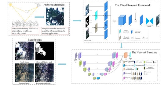
:Pixels of clouds and cloud shadows in a remote sensing image impact image quality, image interpretation, and subsequent applications. In this paper, we propose a novel cloud removal method based on deep learning that automatically reconstructs the invalid pixels with the auxiliary information from multi-temporal images. Our method’s innovation lies in its feature extraction and loss functions, which reside in a novel gated convolutional network (GCN) instead of a series of common convolutions. It takes the current cloudy image, a recent cloudless image, and the mask of clouds as input, without any requirements of external training samples, to realize a self-training process with clean pixels in the bi-temporal images as natural training samples. In our feature extraction, gated convolutional layers, for the first time, are introduced to discriminate cloudy pixels from clean pixels, which make up for a common convolution layer’s lack of the ability to discriminate. Our multi-level constrained joint loss function, which consists of an image-level loss, a feature-level loss, and a total variation loss, can achieve local and global consistency both in shallow and deep levels of features. The total variation loss is introduced into the deep-learning-based cloud removal task for the first time to eliminate the color and texture discontinuity around cloud outlines needing repair. On the WHU cloud dataset with diverse land cover scenes and different imaging conditions, our experimental results demonstrated that our method consistently reconstructed the cloud and cloud shadow pixels in various remote sensing images and outperformed several mainstream deep-learning-based methods and a conventional method for every indicator by a large margin.
1. Introduction
Satellite-mounted optical sensors offer a great opportunity to conveniently capture the geometric and physical information of the Earth’s surface on a broad scale; however, these sensors are heavily affected by atmospheric conditions, especially clouds. According to the statistics of a USGS study [1], the average global annual cloud coverage is approximately 66%. A large number of satellite images are inevitably covered by clouds and cloud shadows, which restrict subsequent applications such as geo-localization, data fusion, land cover monitoring, classification, and object detection [2]. Hence, repairing shaded pixels has become a practical and important research topic. A variety of cloud removal methods have been designed in the past few decades, which can be simply classified into the two approach categories of conventional and learning-based.
1.1. Conventional Cloud Removal Approaches
Conventional image-based cloud removal methods utilize the information from the neighboring pixels of a cloud region, undamaged bands, cloudless temporal images, or auxiliary information from other sensors to repair current cloudy images with mathematic, physical, or machine learning methods, such as image in-painting technology [3,4], exemplar-based concepts [5,6], interpolation theory [7], and spreading or diffusion model.
Interpolation is a commonly-used technique in cloud removal. Cihlar et al. [8] directly replaced the cloud-contaminated pixels in AVHRR composited images with linear interpolated values. Shuai et al. [9] presented the spectral angle distance (SAD) weighting reconstruction method to interpolate missing pixels. Siravenha et al. [10] applied a nearest-neighbor interpolation together with a DCT-based smoothing method for cloud removal of the satellite images. Yu et al. [11] introduced inverse distance weighted (IDW) interpolation and kriging interpolation to remove the missing pixels of MODIS images. These types of interpolation methods have also been expanded from the spatial domain to the temporal and multi-source domains. For example, Zhang et al. [12] expanded the ordinary cokriging interpolation method from the spatial to the temporal domain to interpolate the values of cloud pixels. Zhu et al. [13] attempted to remove thick clouds based on a modified neighborhood similar pixel interpolation (NSPI) approach from a Landsat time series. Based on a cloudless temporal image and two auxiliary images from another satellite sensor, Shen et al. [14] integrated a modified spatiotemporal fusion method and a residual correction strategy based on a Poisson equation to reconstruct the contextual details of cloud regions and enhance the spectral coherence.
The term in-painting is thought to have originated from computer vision. Mendez-Rial et al. [15] developed an anisotropic diffusion in-painting algorithm for the removal of cloud pixels from hyperspectral data cubes. Cheng et al. adopted an image in-painting technology based on non-local total variation, in which multi-band data were utilized to achieve spectral coherence. Non-local correlation in the spatial domain and low-rankness in the spatial-temporal-temporal domain were considered separately in reference [16] to reconstruct missing pixels. Recently, He et al. [17] designed a new low-rank tensor decomposition method and a total variation model for missing information reconstruction.
Multi-temporal images, a series of images covering the same region but at different times, can provide the real land covers that cannot be seen from a cloud image, and many more studies make use of multi-temporal images and are often called temporal-based methods. In references [18,19,20,21], clouds and shadows were detected first, and thereafter the corresponding patches in the non-cloudy image were used to replace them without considering the spectral differences between the temporal images. Lorenzi et al. [22] implemented an isometric geometric transformation to enrich the candidates for missing pixel repairing and a multi-resolution processing scheme to recover the missing pixels in optical remote sensing images. A new combination of kernel functions in support vector regression was designed with auxiliary radiometric information [23]. Zhang et al. [24] proposed a functional concurrent linear model between cloudy and temporal Landsat 7 images to fill in the missing data. Gao et al. [25] proposed a tempo-spectral angle mapping (TSAM) index in the temporal dimension and then conducted the multi-temporal replacement method based on the index. Chen et al. [26] introduced a spatially and temporally weighted regression (STWR) model and a prior modification term for cloud removal based on a multi-temporal replacement. In reference [27], an auto-associative neural network with principal component transform and stationary wavelet transform (SWT) was designed to remove clouds from temporal images. Wen et al. [28] proposed a coarse-to-fine framework with robust principal component analysis (RPCA) theory for cloud removal in satellite images.
1.2. Learning-Based Cloud Removal Approaches
Learning-based cloud removal technology has undergone rapid development, making it now the mainstream approach for cloud removal. This popularity is not only due to its high-performance but also its relief from the requirements of human intervention and handcrafted feature design. Its use in cloud removal includes sparse representation, random forest, and deep learning.
Two multi-temporal dictionary learning algorithms have been expanded from the original dictionary learning to the recovery of cloud and shadow regions without manually designed parameters [29]. Cerra et al. [30] introduced sparse representation theory into cloud removal and reconstructed the dictionary randomly from the available elements of the temporal image. Xu et al. [31] proposed multi-temporal dictionary learning (MDL) to learn the cloudy areas (target data) and the cloud-free areas (reference data) separately in the spectral domain. Considering the local correlations in the temporal domain and the nonlocal correlations in the spatial domain, Li et al. [32] introduced patch matching-based multi-temporal group sparse representation theory into the missing information reconstruction of optical remote sensing images. Based on the burgeoning compressed sensing theory, Shen et al. [33] proposed a novel Bayesian dictionary learning algorithm to solve the dead pixel stripes in Terra and Aqua images.
Subrina et al. [34] proposed an optical cloud pixel recovery (OCPR) method based on random forest to reconstruct the missing pixels. With the aid of an extreme learning machine (ELM), Chang et al. [35] designed a spatiotemporal-spectral-based smart information reconstruction (SMR) method to recover the cloud-contaminated pixel values.
Different from shallow learning technology, such as sparse representation and ELM, deep learning, as a powerful representation learning method with deep neural layers, has been widely introduced to image restoration for denoising, deblurring, super-resolution reconstruction, and cloud removal, the latter of which is, in essence, a missing information reconstruction problem. Zhang et al. [36] introduced convolutional neural networks (CNNs) to the different tasks of missing information reconstruction and proposed a unified spatial-temporal-spectral framework, which recently was expanded into a spatial-temporal patch-based cloud removal method [37]. Praveer et al. [38] applied generative adversarial networks (GANs) to learn the mapping between cloudy images and cloudless images. Chen et al. [39] learned the content, texture, and spectral information of a missing region separately with three different networks. Gao et al. [40] designed a two-step cloud removal algorithm with the aid of optical and SAR images. Ji et al. designed a self-trained multi-scale full convolutional network (FCN) for cloud removal from bi-temporal images [41].
1.3. Objective and Contribution
Although the recent deep-learning-based methods have boosted the study of cloud removal and represent the state-of-the-art, some critical points have not yet been addressed, specifically, several useful human insights raised from previous conventional studies are not yet reflected in a current deep-learning framework. The designed cloud removal networks resemble the basic and commonly-used convolutional networks, such as a series of plain convolutional layers [36,37,39] or U-Net [40,41], all of which lack deeper consideration of the specific cloud removal task (i.e., a local-region reconstruction problem). On the one hand, all these deep-learning-based methods [36,37,38,39,40,41] did not discriminate between cloud and cloudless regions and used the same convolution operations to extract layers of features without considering the difference between clouds and clean pixels. In fact, a discriminative mechanism considering their distinct features could boost cloud removal performance. Although conventional studies tended to use different empirical features to represent clouds and other regions, it is not exploited in the recent deep-learning-based methods. On the other hand, all these methods [36,37,38,39,40,41] used the single pixel-based loss function at the output space. This type of loss function is commonly used in image semantic segmentation; however, it is insufficient for cloud removal from temporal images for the following reasons. First, the pixel-based loss only matches the valid pixel values of the predicted image and the cloudy image without considering the reconstructed regions. Second, the pixel-based loss lacks a direct mechanism for ensuring color and texture consistency around the reconstructed regions.
For handling the two critical problems, we introduce a novel gated convolutional neural network for extracting spatiotemporal features for high-performance cloud removal in this paper. The main idea and contributions of this work are summarized as follows:
(1) A spatiotemporal based framework for cloud removal is proposed. The network learns the spatiotemporal features from bi-temporal images, a cloudy image, and a clean historical image through a series of gated convolutional layers, which are introduced into cloud removal for the first time in our method. The gated convolutional layers can discriminatively filter out the invalid pixels and encode the abstracted features only from clean pixels for subsequent image repairing, which solves the problem that existed in all the recent deep learning based cloud removal methods [36,37,38,39,40,41] that a common convolutional layer unavoidably encodes information from invalid pixels that would harm the image repairing process. Another notable point is that we use a self-training strategy similar to the work of reference [41] that requires no real training samples but rather requires only clean pixel pairs of bi-temporal images for model training, which is different from [36,37,38,39,40] where real samples had to be prepared through costly and tedious manual work.
(2) We developed a joint loss function that integrates pixel-, feature-, and local-level constraints to strengthen the training process to achieve better global consistency, the ability of loss function is greatly enhanced compared to the mainstream pixel-level loss function [36,37,38,39,40,41]. In particular, the local-level constraint, implemented with a total variation (TV) operation, was designed for the color and texture smoothness of the neighboring pixels of the reconstructed regions. As the gated convolution for discriminating the cloud pixels, the TV loss we designed for smoothness constraint also reflects the beneficial insight from early hand-crafted feature design. The feature-level constraint is implemented through a basic CNN structure, VGG [42], on the assumption that the extracted features from VGG from the original image and the reconstructed image resemble each other.
(3) Minor contributions include the introduction of a multi-scale module, atrous spatial pyramid pooling (ASPP) module, and multi-scale fusion, which aims to expand the receptive field and make full use of the multi-scale features. The other contribution is we apply sub-pixel convolution operation in the multi-scale feature fusion instead of commonly-used upsampling algorithms such as the nearest interpolation and deconvolution to restore more details of irregular clouds.
2. Methods
A spatial-temporal based gated convolutional network (STGCN) was proposed in our method for cloudy image repairing from bi-temporal remote sensing images. The overall framework was detailed in Section 2.1, and the designed network was shown in Section 2.2, Section 2.3, Section 2.4 elaborated the gated convolutions and joint loss, respectively.
2.1. The Overall Framework
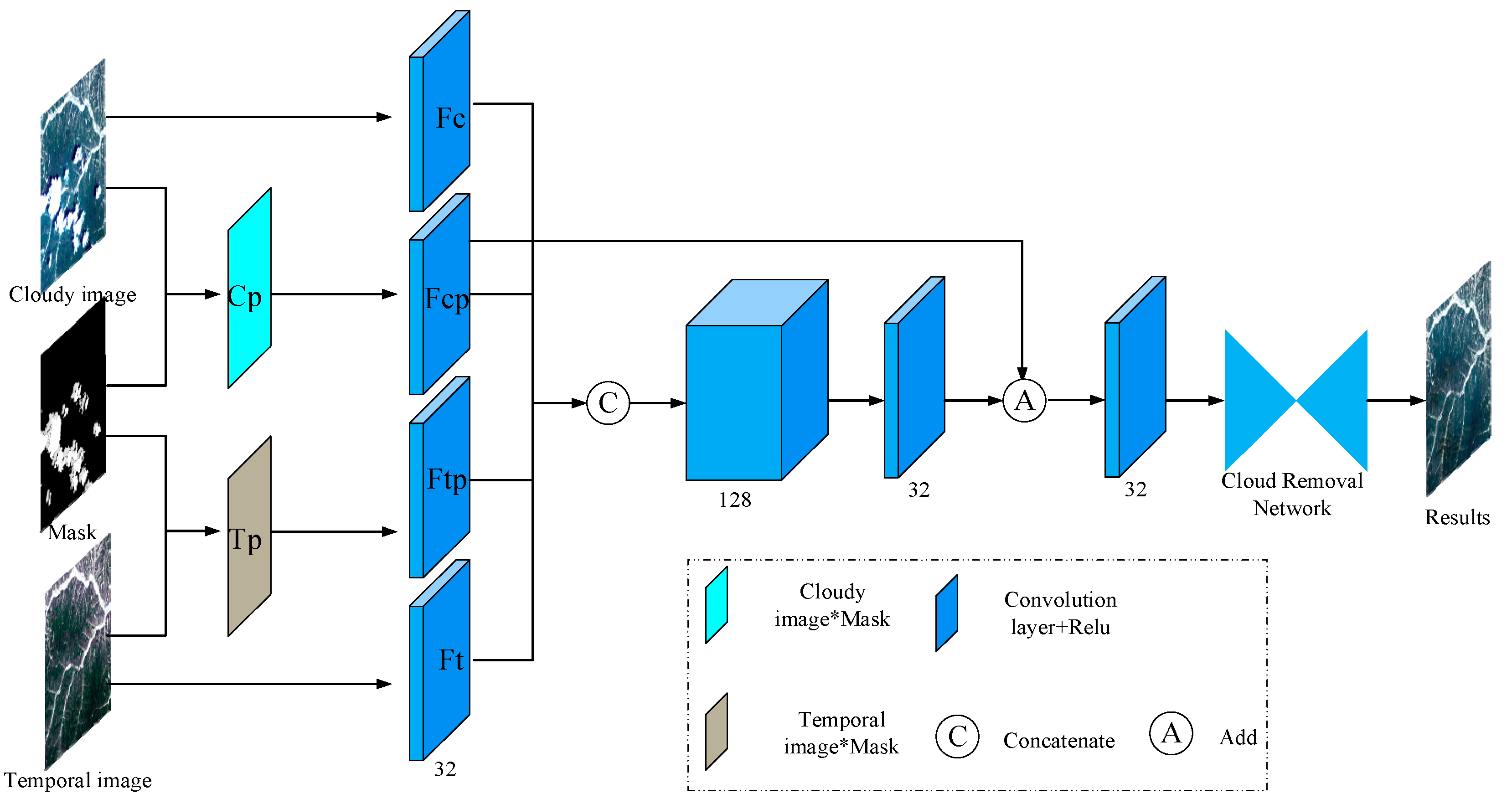
The framework of the proposed STGCN was shown in Figure 1. The current cloudy image, a mask map of clouds and cloud shadows, and a cloudless recent image of the same area were prepared in advance as the input. The mask map, which was a binary map where 1 represented the clean pixels (black), and 0 represents the clouds and cloud shadows (white), can be generated from recent CNN-based detection methods [43,44,45] or manual work. When an automatic algorithm was applied, the recall rate should be set high to detect most of the clouds; however, a relatively lower precision score will not affect the performance of the cloud removal task as a large number of clean pixels remain to train the cloud removal network. The cloudless temporal image can be selected under two conditions: (1) The two images can be accurately geo-registered, and (2) the time span of the two images was not too long for ensuring that no large land cover changes could have happened.
After the input images were prepared, the bi-temporal images were multiplied by the cloud mask map pixel-by-pixel to filter out the cloudy area (denoted as Cp and Tp). The four images, bi-temporal images Cp and Tp, were processed by convolutional layers, each of which consisted of 32 3 × 3 convolution kernels and followed by a ReLU activation. The outputs, denoted as Fc, Fcp, Ft, and Ftp, were concatenated to form a 128-dimension feature map, which was compressed to 32 dimensions by using a 3 × 3 convolution. The 32-dimension feature maps were then concatenated with Fcp and processed by another 3 × 3 convolution layer. The final feature map was sent to the developed cloud removal network.
Our preprocessing had several advantages over directly sending the bi-temporal images and the mask map into the cloud removal network. Firstly, through generating Cp and Tp, we explicitly obtained clean pixels in bi-temporal images, which reduced the learning burden of the cloud removal network. Secondly, the concatenation of features (i.e., Fc, Fcp, Ftp, and Ft) had experimentally shown better performance than the concatenation of original images. Thirdly, the addition operation aimed to enhance the weight of the clean pixels in the cloudy images with the goal of the prediction map from the network and the cloudy image (only clean pixels) being as similar as possible.
2.2. The Cloud Removal Network
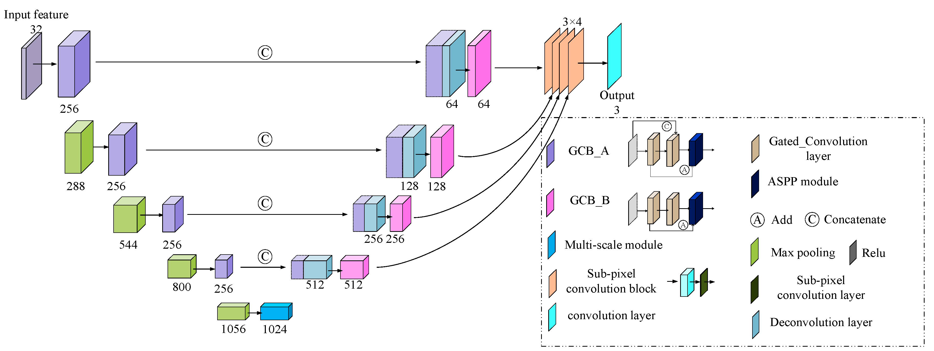
The cloud removal network we propose was shown in Figure 2. The backbone was a classic FCN, as in reference [46] or U-Net [47]. However, each building block was replaced with our gated convolution block (GCB) with skip connections. A multi-scale module at the top of the feature pyramid and a multi-scale feature fusion module before the output layer are were also introduced.
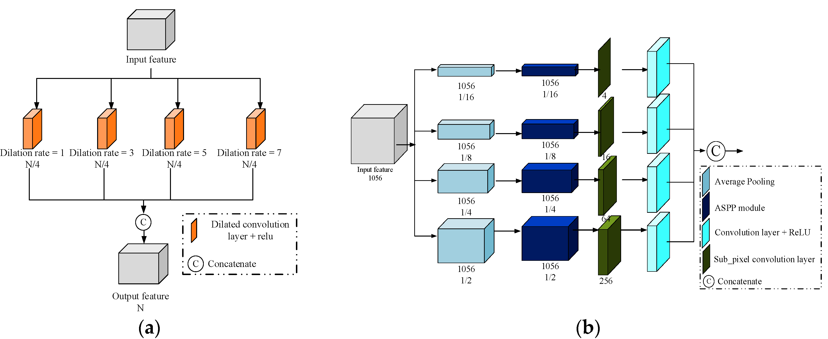
The GCB had two types: (1) Type A (GCB_A, colored with purple) had two skip connections with the first connection a concatenation operator and the second an addition operator; and (2) Type B (GCB_B, colored with pink) had one skip connection with an addition operation, which was only used in the decoder. The last layer of each GCB was an ASPP module (Figure 3a). In the ASPP module, different dilated rates (1, 3, 5, 7) were set to extract the features from different receptive fields, and then the features from the different dilated rates were concatenated.
The multi-scale module at the highest abstraction layer was applied to explore the multi-scale information of the deep features. As shown in Figure 3b, the input feature map was resized to four different sizes (1/2, 1/4, 1/8, 1/16) by average pooling. The features at each scale were then processed by an ASPP module and a sub-pixel convolution layer. The sub-pixel convolutions, instead of direct upsampling, resampled the features at the same scale as the input. Finally, 3 × 3 convolution layers with ReLU were applied, and the output features were concatenated.
In the decoder, the deconvolution layers were used to upsample the features, which were then concatenated to the corresponding features in the encoder and further processed by the GCB_B.
The multi-scale fusion process aggregated information from different spatial scales. The last features at each scale of the decoder were processed by a 1 × 1 convolution layer, followed by a sub-pixel convolution layer to restore the size of the original input. Then, they were channel-wise concatenated and processed by a convolution layer with three channels to obtain the restored cloudy image.
The parameters and super-parameters in the network were set as follows: The stride of the convolution layer was 1, and the kernel size was 3 × 3 in the whole network, except for the specified ASPP module. The rate of max pooling and the stride in the deconvolution layers was 2. The growth rate of the GCB in the encoder was set to 256. The feature dimension of each scale in the decoder was 1024, 512, 256, 128, 64, from top to bottom. For global and local consistency, a joint loss function was used in the training process, which will be described in Section 2.4.
2.3. Gated Convolution Layers
A normal convolution layer functions equally on each pixel of an image, which was suitable for semantic segmentation where each pixel was assigned a category. The similarity between segmentation and image restoring was that they were both pixel-level operations; however, there were explicit invalid pixels in restoring, while in segmentation, there were not. In a deep network, the features extracted from invalid pixels were gradually synthesized to the deeper layers along with the increasing receptive field, which inevitably impacted the restoring quality. Hence, a normal convolution layer can be revised to adapt to this situation by treating valid and invalid pixels separately.
Two special convolutions can treat pixels from an image separately. The first one was called partial convolution. In a partial convolution layer [48], the convolution kernel (i.e., the weight W and bias b) functioned on the combination of an image I and an iteratively-updated binary mask M, in which the value of the invalid pixels was 0. In Equation (1), image I was first multiplied by the mask M element-wisely (denoted by ), and weighted by λ, the ratio of the number of the pixels in mask M and the valid pixel number in M. The mask for the next convolutional layer was automatically updated by a simple rule: If there existed at least one valid value able to condition the output, the location in the mask was updated as valid.
When going deeper into a convolutional network, the valid pixels in the updated mask inevitably were increasing according to the updating rule, which means the side effect of the mask (invalid pixels) was becoming bigger by progressively infiltrating into the valid pixels.
The other convolution was called gated convolution [49], which automatically learns a “soft” mask that discriminates valid and invalid pixels and was different from the empirically-set “hard” mask in partial convolution. Gated convolution is formulated as:
where Wg and Wf are the weights of two different convolutions, bg and bf are the corresponding biases. Ψ is the sigmoid function to make the feature gated between 0 and 1 as the learning mask. The elemental-wise multiplication of feature Φ(F) and the learning mask Ψ(G) is a gated convolution. Sometimes, the feature F can be activated before the multiplication [49]. In (4), Φ can be any activation function such as ReLU [50], LeakyReLU [51], and ELU [52]. Gated convolution can be seen as a generalization of partial convolution. In cloud removal, we utilized gated convolution for discriminating invalid and valid information in each convolutional layer. When the network goes deeper, gated convolution obtains better discrimination ability with a representation learning manner than partial convolution with an empirical setting.
2.4. Joint Loss
The mean square error (MSE) loss for image reconstruction only matched the valid pixel values of the predicted image and the cloudy image. Our proposed loss functions targeted not only pixel-based reconstruction accuracy but also feature level similarity and local smoothing.
As shown in Figure 4, at the image-level, we separately calculated the loss inside and outside the cloudy region. Let Iout represent the reconstruction result, M is the binary mask for clouds and cloud shadows (1 for holes), Igt is the ground truth. The pixel-level losses are calculated as:
At the feature level, we employed a loss function that assessed the similarity between the high-level features of the network output and the ground truth, which was a beneficial supplement of pixel-level similarity. An ImageNet-pretrained VGG-16 [42] was used as a feature extractor to generate high-level features from the network outputs and the ground truth. The loss consisted of two parts. The first part was the L1 distance between the VGG features of the network output and the ground truth. For the second part, we generated a composite image Icomp for addressing the repaired region. The composite image was the linear superposition of the non-cloud region of the ground truth and the mask region of the network output, as shown in Equation (7). The second part was then the L1 distance between the VGG features of the composite image and of the ground truth.
The feature-level loss (perceptual loss) is formulated as:
where Ψn is the activation map of n-th layer of VGG given different inputs. Here, we used layers of pool1, pool2, and pool3 for our loss.
To narrow the gap between the repaired region and the surroundings, i.e., realize the seamless stitching effect of the composited image, we introduced the third loss, which was a smooth function to realize a seamless reconstruction. A total variation (TV) loss was applied as the smoothing penalty of the neighboring region of clouds, as shown in (9).
where (i, j) is the pixel count of the neighboring region P of the cloud outlines. In practice, the neighboring region P can be set as the whole input image, which has been cropped into small tiles (e.g., 256 × 256 pixels) from original remote sensing images for deep-learning-based training and testing.
The final loss was the weighted combination of all the above loss functions. The optimal weights λ is empirically determined by performing a hyper-parameter search.
3. Experiments and Results
3.1. The Experimental Dataset
We selected the open-source WHU Cloud dataset (Supplementary Materials) [41] for our experiments as that dataset covers complex and various scenes and landforms and is the only cloud dataset providing temporal images for cloud repairing. Considering the GPU memory capacity, the six Landsat 8 images in the dataset were cropped into 256 × 256 patches with an overlap rate of 50%. In Table 1, the path and row, the simulated training, validation, testing sample numbers of each data, and the real cloud samples for testing are listed.
The six images have been pre-processed by radiometric and atmosphere correction with ENVI software. Please note that, no real training samples are required in our algorithm, which avoids the high-demand of huge samples for training a common deep-learning model. Instead, all the training samples were automatically simulated on the clean pixels without requiring any manual work. They act actually the same as true samples as providing cloud masks. The simulated samples are used for quantitative training and testing, while the real samples (clouds and cloud shadows) without ground truth (pixels beneath the clouds are never known) are used for qualitative testing.
The adaptive moment estimation (Adam) was used as the gradient descent algorithm and the learning rate was set to 10−4. The training process was iterated 500 epochs each for our model and the other deep learning-based methods to which our model was compared. The weights in (10) were empirically set as λc = 5, λt = 0.5, and λp = 0.06. The algorithm was implemented under the Keras framework of Windows 10 environment, with NVIDIA 11G 1080 Ti GPU.
3.2. Cloud Removal Results
We present our experiments and comparisons of different cloud removal methods: Our proposed STGCN method, the non-local low-rank tensor completion method (NL-LRTC) [16], the recent spatial-temporal-spectral based cloud removal algorithm via CNN (STSCNN) [36], and the very recent temporal-based cloud removal network (CRN) [41]. A partial convolution-based in-painting technology for irregular holes (Pconv) [48] was also executed for quantitative and visual comparison. Except for NL-LRTC, all the other methods are mainstream deep-learning based methods.
The following representative indicators were employed to evaluate the reconstruction results: Structural similarity index measurement (SSIM), peak signal to noise ratio (PSNR), spectral angle mapper (SAM), and correlation coefficient (CC), among which PSNR is regarded as the main indicator. Meanwhile, as the pixels beneath the real clouds could not be accessed, the removal of real clouds was examined with a qualitative assessment (i.e., visual inspections).
Table 2 shows the quantitative evaluation results of different methods on the whole WHU cloud dataset, while Table 3 is the separate evaluation results on different images. As displayed in Table 2 and Table 3, STGCN outperformed the other algorithms for all indicators. Pconv, which was executed only on cloudy images, performed the worst due to the lack of complementary information from temporal images. Although some indexes of the conventional NL-LRTC were sub-optimal, the following reconstructed samples show that it was unstable in some scenes, especially those lacking textures. STSCNN was constructed from an old-fashioned CNN structure, which resulted in the worst performance of the temporal-based methods. CRN was constructed from a similar and popular FCN structure as ours; however, it demonstrated worse performance than ours mainly because CRN could not discriminate between valid and invalid pixels during feature extraction. We use gated convolution for feature extraction. CRN’s inferior performance also was due to two other factors. First, the up-sampling operation with the nearest neighbor interpolation blurred some details. Second, simple MSE loss focused on the similarity of the pixel values exclusively. In contrast, our sub-pixel convolution and the combination of pixel-level, feature-level, and total variation loss contributed to our much better performance. For efficiency, our method requires a little more computational time, which is reasonable as our model is more complicated than those methods with plain convolutions.
Figure 5 shows 12 different scenes, cropped from the six datasets, with huge color, texture, and background differences that could challenge any cloud removal algorithm.
Figure 5a,b originated from data I. In Figure 5a, the regions reconstructed by Pconv and STSCNN, obviously were worse. Pconv introduced incorrect textures and STSCNN handled color consistency poorly. The other three methods showed satisfactory performance both in textural repairing and spectral preservation, although the non-cloud image was very different from the cloud image. However, in the seaside scene (Figure 5b), NL-LRTC performed the worst and basically failed because NL-LRTC only paid attention to the low-rankness of the tensor of the textures while the sea was smooth. Pconv was the second worst performer. Although the results of our method were not perfect, they did exceed the results of all the other methods.
Figure 5c,d originated from data II, which was a city and farmland, respectively. In Figure 5c, none of the repairing results were very good because the temporal image was blurred or hazy. In contrast, in Figure 5d in spite of a bad color match, the temporal image was clear, which guaranteed STSCNN, CRN, and our method obtained satisfactory results. The conventional NL-LRTC performed the worst once again. From these examples, we concluded that the advanced CNN-based methods can fix the problems caused by color calibration but are heavily affected by blurred temporal images, which gives us direction as far as selecting proper historical images for cloud removal.
Figure 5e,f originated from data III and were covered with forests and rivers, where the large parts of randomly simulated clouds challenged the cloud removal results. In Figure 5e, STSCNN, CRN, and STGCN produced satisfactory results in spite of the color bias of the temporal image; and in Figure 5f, CRN and STGCN performed the best. Our method performed the best in both cases. The results and conclusions from Figure 5g,h, which were from data IV and covered with mountains, resembled the results of Figure 5e,f.
Figure 5i,j from data V was an extremely difficult case in that the qualities of both the temporal and cloudy images were low. The three temporal-based CNN networks obtained much better results than the conventional method and single-image based method. The reconstructed results of Figure 5i was relatively worse than that of Figure 5j. This further demonstrates the conclusion from Figure 5c,d: The blurred temporal image Figure 5i heavily affected the reconstruction results, but the color bias of image 5j did not appear to be harmful. Figure 5k,l from data VI covering bare land demonstrated again that our method performed slightly better than the two temporal-based CNNs with the two remaining methods performing the worst.
The performances of different methods for removing real clouds were judged by the visual effects, as shown in Figure 6, for example. First, the clouds and cloud shadows were detected by a cloud detection method called CDN [41]. Then, the mask of the cloud and cloud shadow was then expanded by two pixels to cover the entire cloud area to avoid the damaged pixels involved in training the network. Finally, the CNN-based methods were trained with the remaining clean pixels.
It was observed in Figure 6a that Pconv did not work at all, and there was obvious color inconsistency in the results of STSCNN and apparent texture bias in the results of NL-LRTC. The results from CRN were much better than the former three methods. However, it can be seen from a close review that it blurred the repairing regions, which was largely caused by ignoring the difference between the cloud and clean pixels. Our method exhibited best-repairing performance in all aspects: Color consistency, texture consistency, and detail preservation. In Figure 6b, the results of NL-LRTC, CRN, and our method were visually satisfactory. However, NL-LRTC showed some color bias, which was overly affected by the temporal image. In Figure 6c, the problem occurred again in the NL-LRTC result. Our method performed the best as the repaired region of the second-best CRN was obviously blurred.3.3. Effects of Components
Our cloud removal method STGCN was featured with several new structures or blocks that were not utilized in former CNN-based cloud removal studies. In this section, we demonstrate and quantify the contribution of each introduced structure to the high performance of our method.
3.2.1. Gated Convolution
Conventional convolution treats each pixel equally when extracting layers of features. Gated convolution distinguishes the valid and invalid pixels in cloud repairing and automatically updates the cloud mask through learning. Table 4, where STGCN_CC indicates that common convolution layers replace the gated convolution layers, shows their difference in data I. After introducing the gated convolutions, all of the indicator scores improved, especially the mPSNR score, which increased by 2.3. The significant improvement of PSNR intuitively indicates that the details and textures blurred by common convolutions were repaired by the gated convolutions.
3.2.2. Sub-Pixel Convolution
An up-sampling operation is commonly applied in a fully convolutional network several times to enlarge the compact features up to the size of the original input images. In previous studies, it was mathematically realized by the nearest interpolation, bilinear interpolation, and deconvolution. In this paper, we introduced a sub-pixel convolution to rescale the features, which is also called pixel shuffle. Table 5 shows the powerful effect of sub-pixel convolution. The mPSNR of STGCN was 2.4 higher than STGCN with the nearest interpolation (NI), and 1.2 higher than up-convolution (UC). The effectiveness of sub-convolution may relate to the special object we face: The fractal structure of clouds requires a more exquisite tool to depict the details of the outlines.
3.2.3. Joint Loss Function
Although MSE loss, a pixel-level similarity constraint, was commonly used for CNN-based image segmentation and the inpainting of natural images in computer vision, it was far from enough for the restoration of remote sensing images. This paper introduced a joint loss function that targeted not only pixel-level reconstruction accuracy but also the feature-level consistency and color/texture consistency of the neighboring regions of cloud outlines. Table 6 shows the effectiveness of the perceptual loss designed for feature-level constraint and the TV loss for color consistency. With the optimized weights that were found empirically, the introduction of the new loss component one at a time gradually increased the mPSNR score up to 3.4 growth.
3.2.4. Multi-Scale Module
Table 7 shows the effects of the multi-scale module. When the module for receptive field expanding and multi-scale feature fusion was introduced, there was a slight increase of mPSNR, and the other indicators remained almost the same, which indicated that the module works but was less important than the above three improvements.
3.2.5. Addition Layer
Addition layers were implemented in both of our main building blocks, the GCB_A and GCB_B, in the encoder and decoder, respectively (Figure 7). The base of GCB_A is a ResNet-like block with a short skip connection; and the base of the GCB_B was a series of plain convolution layers. After the additional shortcuts were added to the bases, we saw from Table 8 that the mPSNR score improved by 0.7. As a variation of a skip connection, the addition layer seemed to be effective in cloud removal, which indicated that the frequent short connections, which have widened communication channels between different depths of layers, can improve the performance of a cloud removal network, which resembles the findings in close-range image segmentation or object detection.
4. Discussion
In this section, we discuss the extensions and limitations of our proposed work. First of all, we need one recent cloudless image as auxiliary data. In our experiment, the cloudless image is available from an open-source dataset that was manually constructed. As there are plenty of historical remote sensing images in the same region, developing a pre-processing method to automatically choose a high-quality image may be color-biased but not blurred, as suggested in Section 3.2, is a significant enhancement to bi-temporal or multi-temporal based cloud repairing methods and is a practical manner towards automation.
Second, we used the same data source (Landsat 8), instead of multi-sources, for our experiments. However, the key problem was not rooted in the data sources as we have shown that the appearance differences between the cloudless images and the cloud images, some of which suffered from severe color bias, have no significant impact on cloud repairing. The key factor was pixel-level registration because a deep-learning method learns spectral mapping and cloud repairing from aligned pixel pairs. Therefore, it should be noted that highly accurate geometric registration is necessary before applying a multi-temporal cloud repairing method such as ours.
Third, the strength of our method is in its discrimination ability of two types of pixels (invalid pixels and clean pixels) and its process for handling global and local consistency through the gated convolutions and total variation constraints. Our method is the first introduction of these technologies into deep learning-based cloud repairing. However, they can be applied in any repairing problems related to CNN-based remote sensing image processing.
Finally, this work emphasizes cloud removal instead of cloud detection, and we assume the cloud mask is available or the cloud region can be well extracted by an algorithm. Cloud repairing is, therefore, highly affected by the quality of cloud and cloud shadow masks. The popular cloud detection methods are based on deep learning; however, they still suffer from the lack of enough training samples and strong generalization ability. As a related research topic, the progress of cloud detection will surely benefit most of the cloud removal methods, including ours.
5. Conclusions
In this paper, we presented a novel method that introduces technologies never before used in a deep-learning framework for establishing mapping between the non-cloudy area of a cloudy image and a corresponding cloudless temporal image while at the same time repairing the cloud regions. There are three key technologies employed in our method: (1) Gated convolution layers, which learn how to discriminate cloud and non-cloud regions and automatically update the cloud masks in layers of features; (2) sub-pixel convolution, which replaces the commonly-used up-sampling operation to achieve sub-pixel accuracy; and (3) joint-loss function, which addresses the pixel-level and feature-level similarity and texture and color consistency of repaired regions. Our cloud repairing experiments with bi-temporal images from various scenes demonstrated the robustness of our method and its superiority over other conventional and deep-learning-based methods. The new technologies introduced in this paper can be implemented for other repairing problems involving invalid pixels or emphasizing local spatial and spectral consistency.
Supplementary Materials
The WHU Cloud dataset is available online at http://gpcv.whu.edu.cn/data/.
Author Contributions
Conceptualization, methodology and investigation, P.D. and S.J.; software and validation, P.D.; writing—original draft preparation, P.D. and S.J.; writing—review and editing, P.D., S.J. and Y.Z.; supervision, S.J.; funding acquisition, S.J. and Y.Z. All authors have read and agreed to the published version of the manuscript.
Funding
This work was supported by the National Key Research and Development Program of China, Grant No. 2018YFB0505003.
Conflicts of Interest
The authors declare no conflict of interest.
References
- Zhang, Y. Calculation of radiative fluxes from the surface to top of atmosphere based on ISCCP and other global data sets: Refinements of the radiative transfer model and the input data. J. Geophys. Res. 2004, 109, 1–27. [Google Scholar] [CrossRef] [Green Version]
- Yuan, J. Learning building extraction in aerial scenes with convolutional networks. IEEE Trans. Pattern Anal. Mach. Intell. 2018, 40, 2793–2798. [Google Scholar] [CrossRef]
- Guillemot, C.; Le Meur, O. Image inpainting: Overview and recent advances. IEEE Signal. Proc. Mag. 2014, 31, 127–144. [Google Scholar] [CrossRef]
- Bertalmio, M.; Vese, L.; Sapiro, G.; Osher, S. Simultaneous structure and texture image inpainting. IEEE Trans. Image Process. 2003, 12, 882–889. [Google Scholar] [CrossRef] [PubMed]
- He, K.; Sun, J. Image completion approaches using the statistics of similar patches. IEEE Trans. Pattern Anal. Mach. Intell. 2014, 36, 2423–2435. [Google Scholar] [CrossRef] [PubMed]
- Criminisi, A.; Perez, P.; Toyama, K. Region filling and object removal by exemplar-based image inpainting. IEEE Trans. Image Process. 2004, 13, 1200–1212. [Google Scholar] [CrossRef]
- Rossi, R.E.; Dungan, J.L.; Beck, L.R. Kriging in the shadows: Geostatistical interpolation for remote sensing. Remote Sens. Environ. 1994, 49, 32–40. [Google Scholar] [CrossRef]
- Cihlar, J.; Howarth, J. Detection and removal of cloud contamination from AVHRR images. IEEE Trans. Geosci. Remote Sens. 1994, 32, 83–589. [Google Scholar] [CrossRef]
- Shuai, T.; Zhang, X.; Wang, S.; Zhan, L.; Shang, K.; Chen, X.; Wang, J. A spectral angle distance-weighting reconstruction method for filled pixels of the MODIS Land Surface Temperature Product. IEEE Geosci. Remote Sens. Lett. 2014, 11, 1514–1518. [Google Scholar] [CrossRef]
- Siravenha, A.C.; Sousa, D.; Bispo, A.; Pelaes, E. Evaluating inpainting methods to the satellite images clouds and shadows removing. In Proceedings of the International Conference on Signal Processing, Image Processing and Pattern Recognition (SIP 2011), Jeju Island, South Korea, 8–10 December 2011; pp. 56–65. [Google Scholar]
- Yu, C.; Chen, L.; Su, L.; Fan, M.; Li, S. Kriging interpolation method and its application in retrieval of MODIS aerosol optical depth. In Proceedings of the The 19th International Conference on Geoinformatics (ICG), Shanghai, China, 24–26 June 2011; pp. 1–6. [Google Scholar]
- Zhang, C.; Li, W.; Travis, D.J. Restoration of clouded pixels in multispectral remotely sensed imagery with cokriging. Int. J. Remote Sens. 2009, 30, 2173–2195. [Google Scholar] [CrossRef]
- Zhu, X.; Gao, F.; Liu, D.; Chen, J. A modified neighborhood similar pixel interpolator approach for removing thick clouds in Landsat images. IEEE Geosci. Remote Sens. Lett. 2012, 9, 521–525. [Google Scholar] [CrossRef]
- Shen, H.; Wu, J.; Cheng, Q.; Aihemaiti, M.; Zhang, C.; Li, Z. A spatiotemporal fusion based cloud removal method for remote sensing images with land cover changes. IEEE J. Sel. Top. Appl. Earth Observ. 2019, 12, 862–874. [Google Scholar] [CrossRef]
- Mendez-Rial, R.; Calvino-Cancela, M.; Martin-Herrero, J. Anisotropic inpainting of the hypercube. IEEE Geosci. Remote Sens. Lett. 2012, 9, 214–218. [Google Scholar] [CrossRef]
- Ji, T.-Y.; Yokoya, N.; Zhu, X.X.; Huang, T.-Z. Non-local tensor completion for multitemporal remotely sensed images inpainting. IEEE Trans. Geosci. Remote Sens. 2018, 56, 3047–3061. [Google Scholar]
- He, W.; Yokoya, N.; Yuan, L.; Zhao, Q. Remote sensing image reconstruction using tensor ring completion and total variation. IEEE Trans. Geosci. Remote Sens. 2019, 57, 8998–9009. [Google Scholar] [CrossRef]
- Xu, M.; Jia, X.; Pickering, M. Automatic cloud removal for Landsat 8 OLI images using cirrus band. In Proceedings of the IEEE International Geoscience and Remote Sensing Symposium (IGARSS), Quebec City, Canada, 13–18 July 2014; pp. 2511–2514. [Google Scholar]
- Lin, C.; Lai, K.; Chen, Z.; Chen, J. Patch-based information reconstruction of cloud-contaminated multitemporal images. IEEE Trans. Geosci. Remote Sens. 2014, 52, 163–174. [Google Scholar] [CrossRef]
- Lin, C.; Tsai, P.; Lai, K.; Chen, J. Cloud removal from multitemporal satellite images using information cloning. IEEE Trans. Geosci. Remote Sens. 2013, 51, 232–241. [Google Scholar] [CrossRef]
- Tseng, D.-C.; Tseng, H.-T.; Chien, C.-L. Automatic cloud removal from multi-temporal SPOT images. Appl. Math. Comput. 2008, 205, 584–600. [Google Scholar] [CrossRef]
- Lorenzi, L.; Melgani, F.; Mercier, G. Inpainting strategies for reconstruction of missing data in VHR images. IEEE Geosci. Remote Sens. Lett. 2011, 8, 914–918. [Google Scholar] [CrossRef]
- Lorenzi, L.; Mercier, G.; Melgani, F. Support vector regression with kernel combination for missing data reconstruction. IEEE Geosci. Remote Sens. Lett. 2013, 10, 367–371. [Google Scholar] [CrossRef]
- Zhang, J.; Clayton, M.K.; Townsend, P.A. Missing data and regression models for spatial images. IEEE Trans. Geosci. Remote Sens. 2015, 53, 1574–1582. [Google Scholar] [CrossRef]
- Gao, G.; Gu, Y. Multitemporal landsat missing data recovery based on tempo-spectral angle model. IEEE Trans. Geosci. Remote Sens. 2017, 55, 3656–3668. [Google Scholar] [CrossRef]
- Chen, B.; Huang, B.; Chen, L.; Xu, B. Spatially and temporally weighted regression: A novel method to produce continuous cloud-free landsat imagery. IEEE Trans. Geosci. Remote Sens. 2017, 55, 27–37. [Google Scholar] [CrossRef]
- Tapasmini, S.; Suprava, P. Cloud removal from satellite images using auto associative Neural Network and Stationary Wavelet Transform. In Proceedings of the First International Conference on Emerging Trends in Engineering and Technology, Nagpur, Maharashtra, India, 16–18 July 2008; pp. 100–105. [Google Scholar]
- Wen, F.; Zhang, Y.; Gao, Z.; Ling, X. Two-pass robust component analysis for cloud removal in satellite image sequence. IEEE Geosci. Remote Sens. Lett. 2018, 15, 1090–1094. [Google Scholar] [CrossRef]
- Li, X.; Shen, H.; Zhang, L.; Zhang, H.; Yuan, Q.; Yang, G. Recovering quantitative remote sensing products contaminated by thick clouds and shadows using multitemporal dictionary learning. IEEE Trans. Geosci. Remote Sens. 2014, 52, 7086–7098. [Google Scholar]
- Cerra, D.; Bieniarz, J.; Beyer, F.; Tian, J.; Muller, R.; Jarmer, T.; Reinartz, P. Cloud removal in image time series through sparse reconstruction from random measurements. IEEE J. Sel. Top. Appl. Earth Observ. 2016, 9, 3615–3628. [Google Scholar] [CrossRef]
- Xu, M.; Jia, X.; Pickering, M.; Plaza, A.J. Cloud removal based on sparse representation via multitemporal dictionary learning. IEEE Trans. Geosci. Remote Sens. 2016, 54, 2998–3006. [Google Scholar] [CrossRef]
- Li, X.; Shen, H.; Li, H.; Zhang, L. Patch matching-based multitemporal group sparse representation for the missing information reconstruction of remote-sensing images. IEEE J. Sel. Top. Appl. Earth Observ. 2016, 9, 3629–3641. [Google Scholar] [CrossRef]
- Shen, H.; Li, X.; Zhang, L.; Tao, D.; Zeng, C. Compressed sensing-based inpainting of Aqua moderate resolution imaging spectroradiometer band 6 using adaptive spectrum-weighted sparse Bayesian dictionary learning. IEEE Trans. Geosci. Remote Sens. 2014, 52, 894–906. [Google Scholar] [CrossRef]
- Subrina, T.; Stephen, C.M.; Milad, H.; Arvin, D.S. Optical cloud pixel recovery via machine learning. Remote Sens. 2017, 9, 527. [Google Scholar] [CrossRef] [Green Version]
- Chang, N.-B.; Bai, K.; Chen, C.-F. Smart information reconstruction via time-space-spectrum continuum for cloud removal in satellite images. IEEE J. Sel. Top. Appl. Earth Observ. 2015, 8, 1898–1912. [Google Scholar] [CrossRef]
- Zhang, Q.; Yuan, Q.; Zeng, C.; Li, X.; Wei, Y. Missing Data Reconstruction in Remote Sensing Image With a Unified Spatial–Temporal–Spectral Deep Convolutional Neural Network. IEEE Trans. Geosci. Remote Sens. 2018, 56, 4274–4288. [Google Scholar] [CrossRef] [Green Version]
- Zhang, Q.; Yuan, Q.; Li, J.; Li, Z.; Shen, H.; Zhang, L. Thick cloud and cloud shadow removal in multitemporal imagery using progressively spatio-temporal patch group deep learning. ISPRS-J. Photogramm. Remote Sens. 2020, 162, 148–160. [Google Scholar] [CrossRef]
- Singh, P.; Komodakis, N. Cloud-Gan: Cloud Removal for Sentinel-2 Imagery Using a Cyclic Consistent Generative Adversarial Networks. In Proceedings of the IEEE International Geoscience and Remote Sensing Symposium (IGARSS), Valencia, Spain, 22–27 July 2018; pp. 1772–1775. [Google Scholar]
- Chen, Y.; Tang, L.; Yang, X.; Fan, R.; Bilal, M.; Li, Q. Thick Clouds Removal From Multitemporal ZY-3 Satellite Images Using Deep Learning. IEEE J. Sel. Top. Appl. Earth Observ. 2020, 13, 143–153. [Google Scholar] [CrossRef]
- Gao, J.; Yuan, Q.; Li, J.; Zhang, H.; Su, X. Cloud Removal with Fusion of High Resolution Optical and SAR Images Using Generative Adversarial Networks. Remote Sens. 2020, 12, 191. [Google Scholar] [CrossRef] [Green Version]
- Ji, S.; Dai, P.; Lu, M.; Zhang, Y. Simultaneous Cloud Detection and Removal From Bitemporal Remote Sensing Images Using Cascade Convolutional Neural Networks. IEEE Trans. Geosci. Remote Sens. 2020, 1–17. [Google Scholar] [CrossRef]
- Simonyan, K.; Zisserman, A. Simonyan;, K.; Zisserman;, A., Very Deep Convolutional Networks for Large-Scale Image Recognition. In Proceedings of the International Conference on Learning Representations(ICIL), San Diego, CA, Canada, 7–9 May 2015; pp. 1409–1556. [Google Scholar]
- Qin, M.; Xie, F.; Li, W.; Shi, Z.; Zhang, H. Dehazing for Multispectral Remote Sensing Images Based on a Convolutional Neural Network With the Residual Architecture. IEEE J. Sel. Top. Appl. Earth Observ. 2018, 11, 1645–1655. [Google Scholar] [CrossRef]
- Shao, Z.; Pan, Y.; Diao, C.; Cai, J. Cloud Detection in Remote Sensing Images Based on Multiscale Features-Convolutional Neural Network. IEEE Trans. Geosci. Remote Sens. 2019, 57, 4062–4076. [Google Scholar] [CrossRef]
- Yang, J.; Guo, J.; Yue, H.; Liu, Z.; Hu, H.; Li, K. CDnet: CNN-Based Cloud Detection for Remote Sensing Imagery. IEEE Trans. Geosci. Remote Sens. 2019, 57, 6195–6211. [Google Scholar] [CrossRef]
- Jonathan, L.; Evan, S.; Trevor, D. Fully Convolutional Networks for Semantic Segmentation. IEEE Trans. Pattern Anal. Mach. Intell. 2015, 39, 640–651. [Google Scholar]
- Ronneberger, O.; Fischer, P.; Brox, T. U-net: Convolutional networks for biomedical image segmentation. In Proceedings of the 18th International Conference on Medical Image Computing and Computer-Assisted Intervention (MICCAI), Munich, Germany, 5–9 October 2015; pp. 234–241. [Google Scholar]
- Liu, G.; Reda, F.A.; Shih, K.J.; Wang, T.-C.; Tao, A.; Catanzaro, B. Image Inpainting for Irregular Holes Using Partial Convolution. In Proceedings of the European Conference on Computer Vision (ECCV), Munich, Germany, 8–14 September 2018; pp. 85–100. [Google Scholar]
- Yu, J.; Yang, J.; Shen, X.; Lu, X.; Huang., T. Free-Form Image Inpainting with Gated Convolution. In Proceedings of the Computer Vision and Pattern Recognition (CVPR), Long Beach, CA, Canada, 16–20 June 2019; pp. 4471–4480. [Google Scholar]
- Vinod Nair, G.H. Rectified Linear Units Improve Restricted Boltzmann Machines. In Proceedings of the 27th International Conference on Machine Learning(ICML), Haifa, Israel, 21–24 June 2010; pp. 807–814. [Google Scholar]
- Andrew, L.; Maas, A.Y.H.; Andrew, Y. Ng Rectifier Nonlinearities Improve Neural Network Acoustic Models. Proc. Icml. 2013, 30, 3. [Google Scholar]
- Clevert, D.A.; Unterthiner, T.; Hochreiter, S. Fast and accurate deep network learning by exponential linear units(ELUS). arXiv 2015, arXiv:1511.07289. [Google Scholar]
Figure 1.
The overall framework. Cp and Tp are results of the bi-temporal images being multiplied by the cloud mask map pixel-by-pixel to filter out the cloudy area. Fc, Fcp, Ftp, and Ft are features extracted from cloudy image, Cp, Tp, and temporal image with 32 3 × 3 convolution kernels, respectively.

Figure 2.
The structure of the network. The traditional convolution layers are replaced by the gated convolution layers with two types GCB_A (purple) and GCB_B (pink). A multi-scale module (sky blue) is applied at the top of the encoder, and a multi-scale fusion is introduced to concatenate the last features of different scales of decoder, which are upsampled with sub-pixel convolution blocks (orange) respectively.

Figure 3.
Sub-modules in the network. (a) The atrous spatial pyramid pooling (ASPP) module. (b) The multi-scale module.
Figure 3.
Sub-modules in the network. (a) The atrous spatial pyramid pooling (ASPP) module. (b) The multi-scale module.

Figure 4.
Joint loss that consists of an image-level, a feature level, and a total variation constraint. The image-level constraint includes the loss inside (loss-cloudy) and outside (loss-noncloudy) the cloudy region, the feature-level constraint consists of two perceptual losses.
Figure 4.
Joint loss that consists of an image-level, a feature level, and a total variation constraint. The image-level constraint includes the loss inside (loss-cloudy) and outside (loss-noncloudy) the cloudy region, the feature-level constraint consists of two perceptual losses.

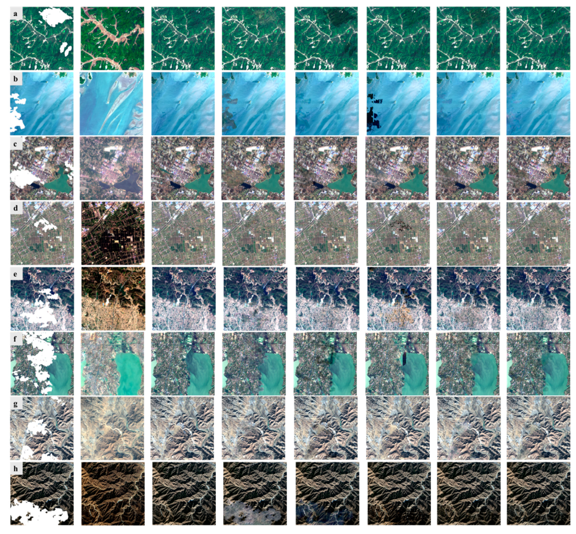
Figure 5.
Comparison of cloud removal results predicted from different methods in different scenes of WHU cloud dataset. (1) Simulated cloudy image. (2) Temporal image. (3) Label. (4) Pconv. (5) spatial-temporal-spectral based cloud removal algorithm via CNN (STSCNN). (6) non-local low-rank tensor completion method (NL-LRTC) (7) cloud removal network (CRN). (8) spatial-temporal based gated convolutional network (STGCN). (a) and (b) are samples from data I, (c,d) from data II, (e,f) from data III, (g,h) from data IV, (i,j) from data V, and (k,l) from data VI.


Figure 6.
Comparison of cloud removal results predicted from different methods. (1) Real cloudy image. (2) Clouds and cloud shadows mask detected from CDN with high recall. Cloud shadows are marked by gray, and clouds are marked by white. (3) Mask after expansion operation. All invalid pixels are marked by white. (4) Temporal image. (5) Pconv. (6) STSCNN. (7) NL-LRTC. (8) CRN. (9) STGCN. (a–c) are repaired samples of real cloud images from different scenes.

Figure 7.
GCB_A block and GCB_B block with and without the addition layer. (a) GCB_A with addition layer; (b) GCB_A without addition layer; (c) GCB_B with addition layer; (d) GCB_B without addition layer.
Figure 7.
GCB_A block and GCB_B block with and without the addition layer. (a) GCB_A with addition layer; (b) GCB_A without addition layer; (c) GCB_B with addition layer; (d) GCB_B without addition layer.


Table 1.
Introduction of WHU Cloud Dataset.
| Data | Path/Row | Simulated Samples | Real Samples | ||
|---|---|---|---|---|---|
| Train | Validation | Test | |||
| I | 118/032 | 576 | 126 | 144 | 27 |
| II | 119/038 | 747 | 180 | 127 | 19 |
| III | 123/039 | 780 | 192 | 152 | 15 |
| IV | 124/033 | 899 | 216 | 180 | 13 |
| V | 126/035 | 616 | 151 | 126 | 104 |
| VI | 127/034 | 718 | 346 | 200 | 30 |
Table 2.
Average quantitative evaluation of different algorithms on simulated clouds of the whole WHU dataset. The best value of each indicator is bolded.
Table 2.
Average quantitative evaluation of different algorithms on simulated clouds of the whole WHU dataset. The best value of each indicator is bolded.
| Method | mPSNR ↑ | mSSIM ↑ | mSAM ↓ | mCC ↑ | Time Efficiency | |
|---|---|---|---|---|---|---|
| Training | Test | |||||
| STSCNN [36] | 31.445 | 0.974 | 5.1823 | 0.9908 | 14 h 39 m | 13s |
| CRN[41] | 32.337 | 0.9768 | 5.1756 | 0.9887 | 14 h 52 m | 7s |
| Pconv[48] | 27.213 | 0.9425 | 5.8851 | 0.9601 | 18 h 49 m | 5s |
| NL-LRTC[16] | 34.115 | 0.9807 | 5.1455 | 0.9806 | / | 9 h 39 min 28s |
| STGCN | 35.749 | 0.9831 | 5.0919 | 0.9916 | 26 h 2 min | 24 s |
↑: The higher score indicates the better effect. ↓: The lower score indicates the better effect.
Table 3.
Quantitative evaluation of different algorithms on simulated clouds of each data in the WHU dataset. The best value of each indicator is bolded.
Table 3.
Quantitative evaluation of different algorithms on simulated clouds of each data in the WHU dataset. The best value of each indicator is bolded.
| Method | STSCNN [36] | CRN [41] | Pconv [48] | NL-LRTC [16] | STGCN |
|---|---|---|---|---|---|
| Data | mPSNR/mSSIM/mSAM | ||||
| I | 29.056/0.977/4.430 | 30.325/0.985/4.423 | 27.375/0.956/4.962 | 34.458/0.982/4.384 | 36.662/0.988/4.354 |
| II | 30.227/0.966/4.393 | 31.986/0.975/4.369 | 28.605/0.953/4.786 | 33.892/0.984/4.459 | 34.138/0.982/4.322 |
| III | 29.136/0.968/4.169 | 31.554/0.975/4.144 | 26.265/0.944/4.698 | 33.768/0.976/4.100 | 36.225/0.979/4.106 |
| IV | 33.701/0.986/4.450 | 32.955/0.976/4.534 | 27.121/0.940/4.842 | 34.753/0.985/4.462 | 36.052/0.988/4.424 |
| V | 31.514/0.976/6.234 | 31.843/0.980/6.225 | 24.680/0.907/7.627 | 34.173/0.982/6.221 | 34.788/0.984/6.154 |
| VI | 35.040/0.975/7.417 | 35.362/0.971/7.359 | 29.235/0.955/8.395 | 33.647/0.975/7.247 | 36.633/0.980/7.192 |
Table 4.
Quantitative evaluation of cloud removal algorithms based on gated convolution layers and common convolution layers on data I. STGCN_CC indicates gated convolution layers in our STGCN have been replaced by common convolution ones.
Table 4.
Quantitative evaluation of cloud removal algorithms based on gated convolution layers and common convolution layers on data I. STGCN_CC indicates gated convolution layers in our STGCN have been replaced by common convolution ones.
| Method | mPSNR ↑ | mSSIM ↑ | mSAM ↓ | mCC ↑ |
|---|---|---|---|---|
| STGCN | 36.6619 | 0.9877 | 4.3538 | 0.9943 |
| STGCN_CC | 34.3079 | 0.9845 | 4.3734 | 0.9918 |
↑: The higher score indicates the better effect. ↓: The lower score indicates the better effect.
Table 5.
Quantitative evaluation of cloud removal algorithms with different up-sampling methods on data I. w/NI is short for with the nearest interpolation. UC is short for up-convolution.
Table 5.
Quantitative evaluation of cloud removal algorithms with different up-sampling methods on data I. w/NI is short for with the nearest interpolation. UC is short for up-convolution.
| Method | mPSNR ↑ | mSSIM ↑ | mSAM ↓ | mCC ↑ |
|---|---|---|---|---|
| STGCN | 36.6619 | 0.9877 | 4.3538 | 0.9943 |
| STGCN w/NI | 34.2569 | 0.9871 | 4.3628 | 0.9943 |
| STGCN w/UC | 35.4819 | 0.9872 | 4.3551 | 0.9939 |
↑: The higher score indicates the better effect. ↓: The lower score indicates the better effect.
Table 6.
Quantitative evaluation of cloud removal algorithms with different components of loss functions on data I. STGCN_1v5h0.5t means the loss function is the weighted addition of mean square error (MSE) for clear pixels with weight 1, damaged pixels with weight 5, and TV loss with weight 0.5, without the perceptual loss.
| Method | mPSNR ↑ | mSSIM ↑ | mSAM ↓ | mCC ↑ |
|---|---|---|---|---|
| STGCN | 36.6619 | 0.9877 | 4.3538 | 0.9943 |
| STGCN_1v5h0.5t | 34.2403 | 0.9879 | 4.3586 | 0.9944 |
| STGCN_1v5h | 33.7992 | 0.9871 | 4.3719 | 0.9933 |
| STGCN_MSE | 33.2852 | 0.9837 | 4.3753 | 0.9941 |
↑: The higher score indicates the better effect. ↓: The lower score indicates the better effect.
Table 7.
Quantitative evaluation of cloud removal algorithms with and without multi-scale module. w/o is short for without.
Table 7.
Quantitative evaluation of cloud removal algorithms with and without multi-scale module. w/o is short for without.
| Method | mPSNR ↑ | mSSIM ↑ | mSAM ↓ | mCC ↑ |
|---|---|---|---|---|
| STGCN | 36.6619 | 0.9877 | 4.3538 | 0.9943 |
| STGCN w/o MS | 36.2912 | 0.9857 | 4.3543 | 0.9942 |
↑: The higher score indicates the better effect. ↓: The lower score indicates the better effect.
Table 8.
Quantitative evaluation of cloud removal algorithms with and without add operation in each block. w/o is short for without.
Table 8.
Quantitative evaluation of cloud removal algorithms with and without add operation in each block. w/o is short for without.
| Method | mPSNR ↑ | mSSIM ↑ | mSAM ↓ | mCC ↑ |
|---|---|---|---|---|
| STGCN | 36.6619 | 0.9877 | 4.3538 | 0.9943 |
| STGCN w/o Add | 35.9858 | 0.9877 | 4.3603 | 0.9942 |
↑: The higher score indicates the better effect. ↓: The lower score indicates the better effect.
Publisher’s Note: MDPI stays neutral with regard to jurisdictional claims in published maps and institutional affiliations. |
© 2020 by the authors. Licensee MDPI, Basel, Switzerland. This article is an open access article distributed under the terms and conditions of the Creative Commons Attribution (CC BY) license (http://creativecommons.org/licenses/by/4.0/).
Share and Cite
MDPI and ACS Style
Dai, P.; Ji, S.; Zhang, Y. Gated Convolutional Networks for Cloud Removal From Bi-Temporal Remote Sensing Images. Remote Sens. 2020, 12, 3427. https://doi.org/10.3390/rs12203427
AMA Style
Dai P, Ji S, Zhang Y. Gated Convolutional Networks for Cloud Removal From Bi-Temporal Remote Sensing Images. Remote Sensing. 2020; 12(20):3427. https://doi.org/10.3390/rs12203427
Chicago/Turabian StyleDai, Peiyu, Shunping Ji, and Yongjun Zhang. 2020. "Gated Convolutional Networks for Cloud Removal From Bi-Temporal Remote Sensing Images" Remote Sensing 12, no. 20: 3427. https://doi.org/10.3390/rs12203427
Note that from the first issue of 2016, this journal uses article numbers instead of page numbers. See further details here.