1. Introduction
Urban areas are expanding rapidly across the world and currently comprise 54% of the global population, versus 30% in 1950 [
1]. As many as half of the urban areas with populations exceeding 100,000 people are water-stressed, which can require expensive methods of desalination or long-distance water transport to supply water [
2]. Studies have shown that 59–67% of residential water use is used for lawn irrigation in urban and suburban areas of the semiarid Southwestern United States [
3]. As such, understanding the full extent and distribution of irrigated land in urban areas will be critical for tracking urban irrigated land use change and developing sustainable water use practices. However, previous classifications of irrigated vegetation have mainly focused on large-scale non-urban agricultural regions [
4,
5,
6].
Irrigation and water use patterns are highly complex in heterogeneous urban areas like the southern California Air Basin (SoCAB). For example, vegetation in the urban core of Los Angeles consists largely of turfgrass and non-native plants, whereas vegetation in non-urban areas and national forests surrounding the city are characterized by native drought-tolerant Mediterranean evergreen and drought-deciduous communities, such as chaparral and coastal sage scrub [
7]. In the City of Los Angeles, lawn irrigation accounts for up to 70% of outdoor landscaping water use, making turfgrass irrigation a frequent target for state mandates to reduce water usage during extended drought conditions [
7]. Across all of California, outdoor water use is dominated by turfgrass irrigation and can account for over half of residential water use [
8]. In addition to lawns near residential housing, turfgrass is commonly found at golf courses, cemeteries, and school fields, which can dominate large fractions of the urban landscape [
3].
The heavy reliance on irrigation for urban landscaping results in outdoor residential water use peaking during the summer, when evaporative demand and potential water loss spike, and regional drought conditions limit water supply [
9]. Consequently, the non-irrigated vegetation in SoCAB experiences a cyclical cycle of greening in the late winter and early spring, followed by summer senescence, while irrigated vegetation typically stays green throughout the year [
10]. As such, an accurate map of urban irrigated vegetation is critical for accurately modeling local and regional hydrological cycles [
11].
These differences in irrigated and non-irrigated vegetation productivity have a substantial influence on local climate and energy use. A growing field of research suggests that irrigation has a strong cooling effect on vegetation that is most pronounced in semi-arid and arid climates and can be measured using remotely sensed land surface temperature (LST) [
12,
13]. This affects stomatal conductance and soil microbial activity, and subsequently evapotranspiration (ET) and ecosystem carbon exchange, through temperature sensitivity [
14,
15]. For example, wealthier neighborhoods in SoCAB consume twice as much water for outdoor irrigation as low-income neighborhoods, producing an evaporative cooling effect, which decreases the LST [
16], heat vulnerability due to reduced urban heat island (UHI) effect [
17], and energy demand [
7]. Neighborhoods in Los Angeles with high irrigation show lower LST than neighborhoods with low irrigation by 3.2 +/− 0.02 K, with the most pronounced difference in late spring and summer [
18]. Similarly, previous studies have found a relationship between LST, vegetation presence, and productivity in the urban areas of Shanghai [
19]. These relationships suggest that LST can provide a valuable signal for classifying irrigated vs. non-irrigated vegetation across SoCAB and detecting drought stress across urban and non-urban areas.
Previous efforts to classify land use in irrigated areas have typically focused on agricultural regions, which consist of relatively large fields spanning hundreds of hectares, cover a large portion of the United States and other nations, and can account for the majority of freshwater use. Bousbih et al. (2018) used Sentinel-1 Synthetic Aperture Radar (SAR) C-band and Sentinel-2 multi-spectral optical imagery to map soil moisture and irrigated land in a semi-arid agricultural region of Tunisia, producing an accuracy of 72% compared to ground truth measurements. Qi et al. (2002) [
20] used 1992 Landsat 5 multi-spectral optical imagery to classify irrigated crop lands in the High Plains aquifer region of the United States at a 30 m resolution and with 77.5% weighted accuracy. Similarly, Chance et al. (2017) used Moderate Resolution Imaging Spectroradiometer (MODIS) and Landsat 5 optical imagery to distinguish between irrigated and non-irrigated land in the semi-arid agricultural Snake River Plain in Idaho with accuracies varying from 86% to 95% depending on the sensor and spectral vegetation index used.
Earlier attempts to classify irrigated vs. non-irrigated vegetation and other vegetation land use parameters with LST data have been limited by the coarse spatial resolution of MODIS LST (1 km), which is insufficient for resolving mixed pixels in a heterogeneous urban environment. Some studies of water use and irrigated vegetation in urban areas have relied on a combination of aerial optical imagery, field surveys, and water bills. For example, Johnson and Belitz (2012) used linear mixture analysis with Landsat Thematic Mapper 5 Normalized Difference Vegetation Index (NDVI) and monthly landscape ET rate calculated from a nearby California Irrigation Management System station to estimate the monthly rate of irrigation and the fraction of irrigated landscaping in the San Fernando Valley at 30 m resolution. However, this study only covered a smaller subset of SoCAB and only accounted for three landcover types—impervious surface, irrigated vegetation, and non-irrigated vegetation—which fails to account for potential differences in irrigation patterns between urban trees and urban turfgrass.
Our work extended the study area of Johnson and Belitz (2012) by more than double their extent to include all of SoCAB and demonstrated the utility of using a high-resolution urban landcover map to “unmix” coarser LST imagery for distinguishing between irrigated and non-irrigated vegetation in a heterogeneous urban environment. The high-resolution urban landcover map included four landcover types relevant to our study: grass, tree, shrub, and non-photosynthetic vegetation (NPV)/bare soil [
21]. Our algorithm used a vegetation fraction weighted LST product derived from this high-resolution landcover map and sharpened LST from the ECOsystem Spaceborne Thermal Radiometer on Space Station (ECOSTRESS, 30 m sharpened). We validated the algorithm using two independent datasets and compared this product to classifications of irrigated vs. non-irrigated areas using more traditional RGB-NIR and NDVI spectral signatures from Landsat 8 (30 m), Sentinel-2 (10 m), and National Agriculture Imagery Program (NAIP, 0.6 m) optical imagery.
2. Methods
This study developed a method to distinguish between irrigated and non-irrigated vegetation that is accurate in both heterogeneous urban environments and unmanaged wildlands, using SoCAB as a test case. The following sections describe our classification scheme in more detail, including a brief description of ECOSTRESS data in
Section 2.1 and
Section 2.2, a methodology to resolve mixed pixels in
Section 2.3, and the selection of other base imagery for comparing classifications in
Section 2.4. The workflow for supervised classification to distinguish between irrigated and non-irrigated section is broken into three main sections (
Figure 1). Training data selection is addressed in
Section 2.5, and classifier training and validation are addressed in
Section 2.6.
2.1. Data from ECOSTRESS
ECOSTRESS has been actively collecting data since July 2018, measuring thermal infrared (TIR) radiation in five bands spanning the 8 to 12.5 μm wavelength range [
22]. ECOSTRESS is installed on the International Space Station (ISS), which has a precessing orbit that leads to sporadic spatial and temporal sampling with revisit frequencies of between 3–5 days depending on latitude and acquisition at varying times of the day. ECOSTRESS pixels have a spatial resolution of 70 × 70 m at nadir. Our land use classification used the Level-1B geolocation data (L1BGEO), the Level-2 LST (ECO2LSTE), the Level 2 cloud product (ECO2CLOUD), and the Level 4 evaporative stress index (ESI) product (ECO4ESI). The standard LST product was recently validated to an accuracy of 1.07 K in RMSE at fourteen global sites consisting of vegetation, water, and soils [
23].
Because the aim of this classification procedure was to distinguish between irrigated and non-irrigated landcover in SoCAB, we used ECOSTRESS imagery from late summer (July, August, September). While the majority of SoCAB is not covered by irrigated cropland, seasonal patterns in irrigation of managed landscapes (e.g., residential/commercial lawns and gardens, parks, golf courses, cemeteries) lead to peak water usage during the dry summer months. Furthermore, past studies have shown the difference in NDVI between irrigated and non-irrigated vegetation is most pronounced at the peak of the growing season for semi-arid agricultural areas [
5,
24].
The variable ECOSTRESS overpass times were leveraged to identify the time of day during summer (July, August, and September) that maximized the difference in LST between irrigated and non-irrigated vegetation. After randomly selecting 100 irrigated and 100 non-irrigated pixels across SoCAB, the AppEEARS tool (
https://lpdaac.usgs.gov/tools/appeears/) was used to extract a time series of ECOSTRESS LST values during summer 2018 and summer 2019. This data was used to determine that afternoon periods between 1–3 pm local time showed the most significant difference in LST between irrigated and non-irrigated vegetation. Based on this result, we used 7 ECOSTRESS LST images from July-September between these hours.
2.2. Pre-Processing ECOSTRESS LST Imagery
The corresponding ECO2CLOUD mask was applied to each of the ECOSTRESS LST images, removing all pixels that were classified as clouds. The 7 clear-sky ECOSTRESS LST scenes were then stacked and averaged on a pixel-by-pixel basis. The final pre-processed ECOSTRESS product consisted of a 30 m sharpened composite LST product across SoCAB and cropped to the desired study area. During the morning summer months, a marine layer forms along coastal southern California regions (termed “June gloom”), obscuring the coast of Los Angeles in low altitude stratus clouds that typically burn off by noon. These clouds were clearly visible in all summer morning ECOSTRESS LST imagery, making it difficult to create a fully cloud-free LST morning image in SoCAB. A preliminary investigation into the standard ECOSTRESS cloud mask indicated that while it masked out the majority of clouds in southern California, it often failed to mask out low-lying warm clouds since the algorithm is based on thermal tests only. Based on averaged NOAA climatic data, downtown Los Angeles experiences 1 cloudy day and 9 partly cloudy days in July, 1 cloudy day and 7 partly cloudy days in August, and 3 cloudy days and 8 partly cloudy days in September. As such, cloud cover was not a major issue for the selected afternoon summer period in Los Angeles (July, August, September), but this assumption may not hold in other urban areas.
After cloud-masking, the ECOSTRESS LST images were sharpened from a 70 × 70 m to 30 × 30 m spatial resolution to distinguish between irrigated and non-irrigated vegetation in the heterogeneous Los Angeles megacity. The native resolution of ECOSTRESS LST imagery is 70 × 70 m at nadir but degrades to ~100 m at the edge of the swath due to higher view angles. While this spatial scale is typically sufficient for recognizing irrigated vs. non-irrigated features in non-urban agricultural regions, it is too coarse to pick up fine-scale irrigated features in a heterogeneous urban environment like Los Angeles. Sharpening ECOSTRESS LST imagery to 30 m × 30 m allows for clearer visualization of irrigated landmarks, such as cooler golf courses and parks in green and blue (
Figure 2). A higher resolution LST product makes it possible to train a supervised classifier to distinguish between irrigated vs. non-irrigated vegetation, even in a heterogeneous environment.
We used a LST sharpening algorithm optimized for urban environments that is currently being used to produce a Multi-Source Land Imaging urban LST product for U.S. cities available through the NASA Land Cover Land Use Change (LCLUC) program (see:
https://lcluc.umd.edu/people/glynn-hulley, [
17]). The sharpening algorithm uses a multiple regression model trained on coincident 3 m airborne AVIRIS surface reflectance and Hyperspectral Thermal Emission Spectrometer (HyTES) thermal data [
25] across Los Angeles. The accuracy of the model is ~2.5 K when compared to an independent set of HyTES LST data. An important component of the model is a normalization procedure that ensures that the average of all sub-pixel sharpened LST pixels at 30 m resolution equals the LST of the native resolution pixel at 70 m resolution. The model was used to sharpen ECOSTRESS LST data with Landsat 8 surface reflectance data to 30 m Landsat pixels. Summer 2018 ECOSTRESS images were sharpened using Landsat 8 Tier 1 On-Demand surface reflectance imagery acquired on 31 August, 2018 and summer 2019 ECOSTRESS images were sharpened using Landsat 8 imagery acquired on 19 September, 2019. These dates correspond to a series of mostly cloud-free Landsat 8 images that aligned with the July-September summer time frame of the ECOSTRESS images.
2.3. Resolving Mixed Pixels
Plant canopies vary in size but are typically less than 5 m in width, such that in a heterogeneous urban environment like SoCAB, even a 30 m pixel from Landsat 8 or sharpened ECOSTRESS LST is most likely composed of mixed landcover. A mixed pixel is a pixel that can be decomposed into a linear mixture of spectral endmembers, where an endmember is defined as a “pure” landcover class [
10]. For example, a 30 m mixed pixel in Los Angeles could consist of a combination of impervious surface, grass, and shrub endmembers. As such, we unmixed pixels in the composite ECOSTRESS LST median product by multiplying LST by the fractional vegetation cover (grass, NPV/bare soil, shrub, tree) across SoCAB and used this image in training a supervised classification model. Weighting the ECOSTRESS LST product with fractional vegetation cover made the classification between irrigated and non-irrigated vegetation more distinct. A high-resolution urban landcover map (0.6–10 m) over the same study domain as this classification effort (
Figure 3a; [
21]) was used to account for mixed pixels by calculating the fractional vegetation cover for each 30 m Landsat 8 or ECOSTRESS LST pixel (
Figure 3b). This landcover map was also used to mask all impervious surfaces and water, leaving four vegetated landcover classes: grass, shrub, tree, and NPV/bare soil.
2.4. Pre-Processing VSWIR Data for Irrigated/Non-Irrigated Classification
Optical imagery spanning the visible to shortwave infrared (VSWIR) at variable spatial resolutions from Sentinel-2, Landsat 8, and NAIP was used to compare against the weighted LST-based approach for classifying irrigated and non-irrigated vegetation. The Copernicus Sentinel-2 VSWIR multi-spectral radiometer has a high spatial resolution (10–60 m and 440–2200 nm wavelength) and frequent revisit period (3–5 days in midlatitudes). Sentinel-2 Level 1C imagery provides top-of-atmosphere (TOA) reflectance in cartographic geometry and has been radiometrically and geometrically corrected [
26]. The US Geological Survey Landsat 8 imagery has a moderate spatial resolution (30 m), revisit time (16 days), and 9 spectral bands spanning 430–2290 nm. The Google Earth Engine (GEE,
https://earthengine.google.com) catalog contains Collection 1 Tier 1 Landsat 8 calibrated TOA reflectance. NAIP airborne imagery is delivered by the US Department of Agriculture Farm Service Agency to provide leaf-on imagery over the continental US during the growing season and is freely and publicly accessible at either a 60 cm or 1 m resolution. Like most states, California’s NAIP imagery contains four spectral bands (red, green, blue, and near-infrared) at 60 cm resolution and is re-acquired every two to four years (2008, 2012, 2016, and 2018).
The frequent revisit time of Sentinel-2 and Landsat 8 imagery means that it is possible to minimize shadow effects by calculating the per pixel median spectral signature for RGB-NIR bands during our study period. Using a median-derived optical composite image also helps exclude both high and low spectral reflectance values that can complicate supervised classification efforts, corresponding to snow/clouds/albedo and shadows, respectively [
21]. This classification calculated the median per pixel value from July–September 2018 across SoCAB of Sentinel-2 imagery (262 images) and Landsat 8 imagery (33 images). The median image was treated as a single mosaicked RGB-NIR image to train a supervised random forest classifier. All classification efforts were completed in GEE in May–June 2020 using built-in NAIP, Level 1C Sentinel-2 data, and Landsat 8 Collection 1 Tier 1 TOA Reflectance under the Earth Engine image collection snippets for “USDA/NAIP/DOQQ”, “COPERNICUS/S2”, and “LANDSAT/LC08/C01/T1_TOA”, respectively. GEE is a cloud-based platform for geospatial data analysis and the Javascript application programming interface (API) provided both access to the necessary data sets and an efficient way to classify and export the entire study region [
27].
2.5. Selection of Irrigated and Non-Irrigated Training Data
This classification relied on hand-drawn polygons across SoCAB for the irrigated and non-irrigated landcover classes to train and validate the irrigated/non-irrigated landcover classification model. A total of 402 irrigated and 760 non-irrigated polygons were drawn from 0.6 m 2016 NAIP imagery in QGIS 3.10. Irrigated training polygons covered 2.71 km2 and non-irrigated training polygons covered 44.34 km2 across SoCAB. Irrigated training data was largely drawn from cemeteries and golf courses in SoCAB, and it was assumed that all green-appearing grass was irrigated. Non-irrigated training data was drawn from non-irrigated urban land (i.e., senescent vegetation) and the unmanaged wildlands across SoCAB.
Irrigated and non-irrigated polygons were randomly split into 80% training and 20% validating collections to ensure that the 40,000 training and validating data points were independent. Of the 20,000 irrigated points, 16,000 training points were randomly selected leaving 4000 randomly selected for validation. Similarly, for the 20,000 non-irrigated points, 16,000 training points were randomly selected leaving 4000 randomly selected for validation. The validation accuracy was calculated using the hold-out irrigated/non-irrigated validating data set that was not used for training the supervised classification model.
Because this classification utilizes imagery from multiple years (2016, 2017, 2018, and 2019), we removed training and validating points that experience substantial interannual changes in NDVI. Drought conditions across SoCAB vary greatly between subsequent years, with much of the basin under exceptional drought conditions in September 2016, abnormally dry to moderate drought in September 2017, severe drought in 2018, and no drought in September 2019 [
28]. Furthermore, Los Angeles has residential and commercial water use restrictions that vary based on drought conditions and water supply, which can influence the total area and spatial distribution of irrigated vegetation in SoCAB [
29]. Lastly, agricultural regions of SoCAB utilize crop rotation such that some fields may remain fallow for a growing season and then are photosynthetically active the next year (
Figure 4). As such, points that that had variable spectral signatures between years using the differenced 30 m Landsat 8 NDVI (dNDVI) from year to year (2016–2017, 2017–2018, and 2018–2019) were removed from the training and validating datasets.
2.6. Supervised Model Training and AVIRIS Validation
Four spectral bands (red, green, blue, near-infrared Landsat 8 bands), one vegetation index (Landsat 8 NDVI), and four bands of weighted LST (tree-weighted LST, grass-weighted LST, shrub-weighted LST, NPV/bare soil-weighted LST) were used to train a Smile Random Forest Classifier [
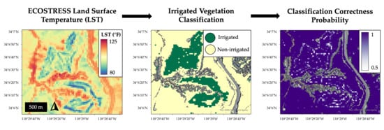
30] with 30 ensembled decision trees. This is the default random forest (RF) algorithm in Google Earth Engine and was used to classify all of SoCAB at 30 m resolution. In addition to the binary irrigated/non-irrigated classification, GEE’s RF implementation outputs the per-pixel probability that a given classification is correct. Thus, we were able to identify the probability that each vegetated pixel was classified correctly as either irrigated or non-irrigated. The typical threshold for defining a pixel as irrigated or non-irrigated in GEE is greater than 0.5, i.e., a pixel with a 0.55 probability of being irrigated is classified as an irrigated pixel.
In addition to performing an accuracy assessment and calculating a confusion matrix from the supervised classification model with the withheld validation data set, our irrigated/non-irrigated vegetation classification was compared against an independent external data set to evaluate consistency between products. Wetherley et al. (2018) developed a 30 m fractional urban landcover map using 2014 Airborne Visible/Infrared Imaging Spectrometer (AVIRIS) imagery in urban areas of SoCAB. This classification included a fractional cover of turfgrass and NPV/bare soil, which were defined as irrigated and non-irrigated for the external validation set, respectively. Irrigated and non-irrigated pixels from the AVIRIS map that varied from 75% to 100% fractional cover were selected, where 100% cover corresponds to a pure irrigated or pure non-irrigated pixel. These data points were combined to create an irrigated/non-irrigated external validation set and to calculate the overall accuracy of our irrigated/non-irrigated landcover classification.
4. Discussion
In this study, we tested different combinations of satellite and aerial imagery to study the feasibility of developing a high-resolution map of irrigated vegetation in a heterogeneous Mediterranean megacity, Los Angeles. Combining landcover-weighted ECOSTRESS LST imagery (30 m) and Landsat 8 optical imagery (30 m) most accurately classified vegetation as irrigated vs. non-irrigated across SoCAB with a 98.2% validation accuracy (classification is available online at
http://dx.doi.org/10.17632/x2zmf7z2zw.2). Weighting the coarser LST imagery with a 30 m fractional aggregation of the high-resolution vegetation map enabled “unmixing” the vegetation fraction in a single ECOSTRESS LST pixel. These mixed pixels may be an important factor in the distribution of urban LST because UHI impacts are driven by a higher fractional coverage of impervious surface and mitigated by a higher fractional coverage of vegetation [
16].
Our method can be replicated for any urban area of the United States where high-resolution vegetation maps are available, ideally at 1 m or less for heterogeneous landscapes. For example, the EPA EnviroAtlas project has openly accessible 1 m landcover classification for 30 U.S. urbanized community areas that cover 1400 cities and towns, including Austin, TX, Chicago, IL, Memphis, TN, New York, NY, Phoenix, AZ, and St. Louis, MO [
31]. Better understanding the distribution of irrigated and non-irrigated vegetation in urban areas can help predict areas susceptible to significant UHI effects or identify targets for reducing urban water use.
4.1. Comparing ECOSTRESS LST in Morning vs. Afternoon
Unlike previous missions for measuring ET and LST at a global scale, the irregular orbit of the ISS means that the overpass return frequency for ECOSTRESS for a given location is 3–5 days, depending on latitude, at different times of day, with the same time of day repeat of approximately 60 days [
22]. This allows us to quantify LST diurnal cycle changes across a longer time span of about 3 months in southern California. There is significant value in establishing a diurnal time series of LST for distinguishing between irrigated and non-irrigated vegetation, as non-irrigated vegetation is expected to experience a higher daily maximum air temperature than irrigated vegetation [
32]. As such, training a classifier on a single period of time (1–3 pm), when daily summer temperature peaks, was sufficient for distinguishing between irrigated and non-irrigated vegetation in SoCAB and reduced the amount of ECOSTRESS imagery needed.
It was expected that irrigated and non-irrigated vegetation will have similar LST values in the morning when atmospheric conditions favor light absorption, photochemistry, and stomatal conductance in both irrigated and non-irrigated vegetation. In particular, atmospheric conditions favoring photosynthesis include relatively low temperature and atmospheric demand, and relatively high soil moisture and boundary layer CO
2 [
33,
34]. During the summer in SoCAB, afternoon temperatures can easily exceed 40° Celsius and cause heat stress cases where soil moisture supply is insufficient to meet high atmospheric demand and maintain leaf water potential. Native semi-arid plants have typically developed isohydric water use strategies to resist drought, such as signaling the closure of leaf stomata, which reduces evaporative cooling and rapidly warms leaf temperatures [
35]. The more-anisohydric irrigated vegetation is able to maintain photosynthesis under high temperatures due to increases in soil moisture supply, thus leading to increased evaporative cooling of LST in the afternoon.
4.2. Influence of Los Angeles County Water Use Restrictions and Drought Years
In 2014, the Metropolitan Water District of Southern California sponsored a program that included rebates for constituents who replaced their lawns with drought-tolerant landscaping, paying up to
$2.00 per square foot for residential lawns [
36]. In 2015, the governor of California called for the removal of 50 million square feet of lawn across the state. The combination of incentives and water use restrictions from state and local governments have accelerated the replacement of 15.3 million square meters of turfgrass and irrigated lawns with drought-tolerant landscaping in Los Angeles [
36]. Although ECOSTRESS imagery was not available when initial rebates for removing lawns were provided, Vahmani and Ban-Weiss, (2016) [
37] determined that the California lawn replacement program resulted in daytime warming of 1.9 °C and a nighttime cooling of 3.2 °C. There continues to be a shift toward reducing residential and business irrigation in Los Angeles. An important area of future research will be change detection of irrigation trends in urban areas, such as looking at vegetation fraction-weighted ECOSTRESS imagery between multiple years as more data becomes available.
In order to acquire sufficient ECOSTRESS LST imagery to cover all of SoCAB after cloud-masking, this classification utilized imagery from summer 2018 and summer 2019. However, there are important concerns with mixing 2018 and 2019 imagery, as the United States Drought Monitor identified that portions of SoCAB were under severe drought conditions from July-September 2018, while the region was drought-free from July-September 2019. Water use restrictions often vary depending on the location of drought conditions, which means that the spatial distribution of irrigated vegetation may change between years. Eliminating training points of the RF classifier that experienced a large change in NDVI between subsequent years did minimize the bias of changing irrigation patterns when training our classifier but does not fully account for combining different years with potentially varying irrigation levels. More research will be needed to better understand how irrigation regimes vary between subsequent years, likely using an imagery source that has a higher afternoon temporal repeat than ECOSTRESS.
In addition, there are some concerns with varying drought conditions between the external validation AVIRIS-derived land cover map (2014 imagery) and our irrigated/non-irrigated classification (2018 and 2019 imagery). 2014 was a serious drought year for SoCAB, with much of the basin under extreme or exceptional drought conditions between July-September, whereas 2018 and 2019 had milder drought conditions. Although there is potential for differences in the spatial distribution of irrigated vegetation across SoCAB between 2014 and 2018–2019 due to varying drought conditions, we performed both this external validation and validation with the hold-out validating points to build additional confidence in our classification.
4.3. Edge Effects and Uncertainty in RF Supervised Classification
Edge effects are a common problem in image classifications, particularly when the analysis window size is large and the window begins to include pixels from adjacent land cover types [
38]. The window size for our irrigated/non-irrigated land use classification map based on LST-weighted sharpened ECOSTRESS imagery is 30 m, which is coarse enough to likely include mixed pixels in a heterogeneous environment like SoCAB. In an accuracy assessment of a thematic landcover map in Brazil, Powell et al. (2004) [
39] determined that 47% of classification disagreements between reference data and a 30 m Landsat Thematic Mapper (TM) landcover map occurred in edge pixels after correcting for geolocation errors. Sweeney and Evans (2012) [
40] assessed error sources in a Landsat TM thematic landcover map of south-central Indiana and determined that both omission and commission errors tended to be higher in edge pixels than in interior pixels.
The RF classifier trained on 30 m vegetation fraction weighted LST and Landsat 8 optical imagery for distinguishing between irrigated and non-irrigated vegetation has the most uncertainty in edge pixels where the landcover type changes from irrigated to non-irrigated. For example, uncertainty is highest along the edges of irrigated agricultural fields, where there are likely mixed pixels that contain a combination of irrigated and non-irrigated vegetation at a 30 m resolution. This makes it more challenging for our RF classifier to confidently determine whether a pixel is irrigated or non-irrigated. A similar effect was identified at urban and suburban golf courses in SoCAB, where uncertainty was highest along the perimeter of the golf course where the base imagery typically shifts from clearly irrigated and homogeneous turfgrass to a more heterogeneous residential environment (
Figure 8).
4.4. Selecting the Best Map for Irrigated Vegetation Mapping in SoCAB
Previous studies of irrigation mapping have tested the efficacy of using multiple satellite sensors versus a single satellite sensor for classification. Bousbih et al. (2018) utilized Sentinel-1 radar data and Sentinel-2 optical imagery to derive soil moisture and NDVI, respectively and determined that a synergistic combination of both sensors was more effective than NDVI alone but less effective than soil moisture alone for detecting irrigated areas. Similarly, Chance et al. (2017) used multiple satellite sensors to identify irrigated areas with multiple spectral indices and found that Landsat (30 m) had higher accuracies than MODIS (250 m). Alexandridis et al. (2008) used a combination of Advanced Spaceborne Thermal Emission and Reflection Radiometer (ASTER), SPOT-4 HRV, and Landsat 7 optical imagery to map irrigated areas in the Mediterranean. These studies did not conclusively determine that using multiple sensors was better or worse for irrigated landcover classification, so we performed our own analysis with single sensors and combined sensors in SoCAB.
Multiple random forest supervised classifiers were trained in Google Earth Engine using a variety of different imagery sources and different combinations of the imagery sources. The spatial resolution of the input imagery varied from 0.6 m (NAIP) to 100 m (ECOSTRESS), and the temporal resolution varied from 3–5 days (Sentinel-2) to 2–3 years (NAIP). The optimal classifier would distinguish between irrigated and non-irrigated vegetation in SoCAB at the highest validation accuracy, finest spatial resolution, most frequent temporal resolution, and lowest classifier uncertainty. Ideally, the classifier would not require a large number of input imagery sources or significant data preprocessing before model training.
Unfortunately, the finest spatial resolution imagery usually has the least frequent revisit. The highest spatial resolution, single-sensor imagery (2018 NAIP RGB-NIR and NDVI) classified irrigated vs. non-irrigated vegetation at 0.6 m resolution, but with a low validation accuracy of 69.2% and a low temporal resolution of 2–3 years. This validation accuracy was not sufficient for distinguishing between irrigated and non-irrigated; as it is expected that an untrained random forest model would have a validation accuracy of 50% with two classes.
Since irrigation practices vary through time [
36], it may be most desirable for a more frequent revisit. The model trained using 10 m Sentinel-2 RGB-NIR and NDVI imagery has a high accuracy of 96.0% and a high temporal resolution of 3–5 days, depending on latitude. The median of all Sentinel-2 pixels between July-September 2018 and July-September 2019 was calculated and used for training this model. Sentinel-2 imagery is globally available, and the high temporal repeat makes it possible to minimize cloud effects, which may be important for cities outside of southern California and other semiarid climate zones. Furthermore, this model required data from a single sensor, thereby streamlining the process and reducing uncertainties associated with sensor-specific characteristics [
41].
Although revisit time may be important for looking at land use change, the single-sensor approach is not the most accurate in this study and may not offer insights into pressing scientific questions. The model with the highest validation accuracy (98.2%) combined Landsat 8 RGB-NIR and NDVI imagery with sharpened ECOSTRESS LST imagery weighted by vegetation fraction. Both Landsat 8 and sharpened LST imagery have a spatial resolution of 30 m. Although this landcover-weighted LST method requires more pre-processing to obtain high accuracy and it takes approximately 3 months to cover the entire region with ECOSTRESS LST imagery, it demonstrates the ability to unmix mixed pixels in a heterogeneous environment. This may be particularly important for helping address questions regarding the efficiency of land use practices at a landscape scale and for investigating relationships between carbon and water cycles [
14,
42].
4.5. Future Applications of Irrigated Vegetation Mapping
One application of the irrigated vs. non-irrigated vegetation map is to aid in accurately and reliably separating fossil and biogenic fluxes in urban regions to track the intended consequences of emissions reduction policies. This is particularly challenging because urban areas have complex structures and highly heterogeneous vegetation and impervious surfaces. Urban green spaces such as parks, golf courses, and cemeteries have a potentially important influence on urban carbon cycling, which can vary substantially within and across individual green spaces due to irrigation practices, landscape fragmentation, and edge effects [
43,
44,
45].
Urban irrigated green spaces may contribute to 20% of CO
2 emissions in Los Angeles, underscoring the importance of accurate quantification of the biospheric CO
2 signal in SoCAB [
46]. The integration of moderate-to-high resolution irrigated area and land cover products with carbon and water cycle models are likely to improve quantification of biospheric CO
2 flux, water use, and cooling in urban environments. As such, we expect that our irrigated vegetation map will enable better estimates of societal impacts of urban heat and water usage. It will also provide data-driven information for policy-makers in greenhouse gas monitoring, reporting, and verification (MRV), as well as urban planners looking to mitigate UHI impacts [
47].
5. Conclusions
This study used multiple imagery sources to develop a map of irrigated vs. non-irrigated vegetation at a 30 m spatial resolution in SoCAB, which covers urban and non-urban areas of Los Angeles, a Mediterranean megacity with diverse and heterogeneous landcover. We determined that training a random forest classifier with a combination of Landsat 8 RGB-NIR/NDVI imagery (30 m) and a weighted sharpened ECOSTRESS LST (30 m) with a fractionally aggregated high-resolution urban vegetation map (0.6–10 m) produced a map of irrigated and non-irrigated vegetation cover in SoCAB with an overall accuracy of 98.2%. Future work will utilize this map to improve urban carbon and water cycle models, as well as tracking urban irrigated land use change as longer-term LST imagery becomes available from ECOSTRESS.
A promising area of future research will be testing and validating our model for distinguishing between irrigated and non-irrigated vegetation in other urban areas. Some major urban areas in the United States have high-resolution landcover maps (e.g., EnviroAtlas) that may be sufficient for deriving a vegetation-weighted ECOSTRESS LST product; these regions could serve as a testbed for determining whether this product works for distinguishing between irrigated and non-irrigated vegetation in cities outside of the Mediterranean climate of Southern California. However, high-resolution landcover maps are not available in many urban regions and may not contain vegetation classes that are optimal for distinguishing between irrigated and non-irrigated vegetation. In urban regions that lack an openly-available and high-resolution landcover map, we recommend using Sentinel-2 RGB-NIR/NDVI imagery (10 m) to train a random forest classifier to classify irrigated and non-irrigated vegetation.
The methodology outlined in this study for distinguishing between irrigated and non-irrigated vegetation relied heavily on hand-drawn training and validation data that was specific to the study area. Creating hand-drawn training polygons or collecting ground-truth validation data using high-resolution aerial imagery is time-consuming and can introduce additional uncertainty if there is a temporal mismatch between the high-resolution aerial imagery and the data being used to train a classifier. As such, an important area of future work in irrigated area mapping with remotely-sensed LST or optical imagery will be developing a methodology that relies less heavily on training data specific to the study area. Another approach is to aggregate hand-drawn datasets from different studies, standardizing inputs, and making them openly and publicly available. Alternatively, future research could focus on scaling widely collected field data of water meters from individual lots for comparison to coarser spatial resolution remote sensing data.


