Analyses of Namibian Seasonal Salt Pan Crust Dynamics and Climatic Drivers Using Landsat 8 Time-Series and Ground Data


1
Helmholtz Center Potsdam, GFZ German Research Center for Geosciences, Section 1.4: Remote Sensing and Geoinformatics, Telegrafenberg, 14473 Potsdam, Germany
2
Institute of Geoscience, University of Potsdam, Karl-Liebknecht-Str. 24-25, 14476 Potsdam, Germany
*
Author to whom correspondence should be addressed.
Remote Sens. 2020, 12(3), 474; https://doi.org/10.3390/rs12030474
Submission received: 31 December 2019
/
Revised: 21 January 2020
/
Accepted: 28 January 2020
/
Published: 3 February 2020
(This article belongs to the Special Issue Remote Sensing in Dryland Assessment and Monitoring)
Abstract
:Salt pans are highly dynamic environments that are difficult to study by in situ methods because of their harsh climatic conditions and large spatial areas. Remote sensing can help to elucidate their environmental dynamics and provide important constraints regarding their sedimentological, mineralogical, and hydrological evolution. This study utilizes spaceborne multitemporal multispectral optical data combined with spectral endmembers to document spatial distribution of surface crust types over time on the Omongwa pan located in the Namibian Kalahari. For this purpose, 49 surface samples were collected for spectral and mineralogical characterization during three field campaigns (2014–2016) reflecting different seasons and surface conditions of the salt pan. An approach was developed to allow the spatiotemporal analysis of the salt pan crust dynamics in a dense time-series consisting of 77 Landsat 8 cloud-free scenes between 2014 and 2017, covering at least three major wet–dry cycles. The established spectral analysis technique Sequential Maximum Angle Convex Cone (SMACC) extraction method was used to derive image endmembers from the Landsat time-series stack. Evaluation of the extracted endmember set revealed that the multispectral data allowed the differentiation of four endmembers associated with mineralogical mixtures of the crust’s composition in dry conditions and three endmembers associated with flooded or muddy pan conditions. The dry crust endmember spectra have been identified in relation to visible, near infrared, and short-wave infrared (VNIR–SWIR) spectroscopy and X-ray diffraction (XRD) analyses of the collected surface samples. According these results, the spectral endmembers are interpreted as efflorescent halite crust, mixed halite–gypsum crust, mixed calcite quartz sepiolite crust, and gypsum crust. For each Landsat scene the spatial distribution of these crust types was mapped with the Spectral Angle Mapper (SAM) method and significant spatiotemporal dynamics of the major surface crust types were observed. Further, the surface crust dynamics were analyzed in comparison with the pan’s moisture regime and other climatic parameters. The results show that the crust dynamics are mainly driven by flooding events in the wet season, but are also influenced by temperature and aeolian activity in the dry season. The approach utilized in this study combines the advantages of multitemporal satellite data for temporal event characterization with advantages from hyperspectral methods for the image and ground data analyses that allow improved mineralogical differentiation and characterization.
Keywords:
salt pan; playa; spectral analysis; crust; saline pan cycle; evaporites; time-series mapping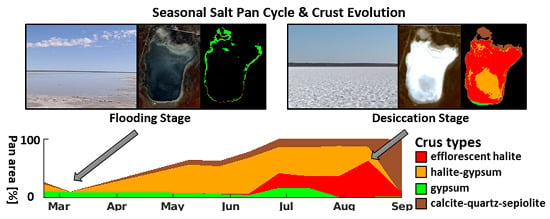
1. Introduction
Salt pan evaporite surfaces are common features in arid regions where closed drainage basins and high evaporation rates favor the development of crusted surfaces mainly composed of evaporite minerals [1]. Although, globally, these landforms occupy limited proportion of the dryland area, they can appear numerous in certain environmental settings, e.g., along paleodrainage lines or in interdune spaces. In parts of Namibia and Southern Africa, salt pans attain densities of up to 1.14 pans/km2 [2] and regionally occupy 20% of the surface area [3]. The surface crust of such salt pans are highly dynamic sedimentary features affected by seasonal-to-interannual changes in rainfall, temperature, and wind ablation [4].
Such salt pan environments have been recognized as a significant sources of mineral dust in arid regions [5,6]. The importance of their dust emissions is illustrated in studies from the western United States [7,8], Australia [9,10], central Asia [11,12], as well as north-central and southern Africa [13,14,15,16,17]. The compositions of dust from these sources can have effects on the climate [18], the degradation of groundwater [19], soil and ocean fertilization [20], as well as human [21] and ecosystem health [22]. Dust type and emissivity are related to the mineralogical and physical crust composition [8,23,24]. The advances in understanding of these dust sources and for modeling dust emissions depend on the characterization of the salt pan surface over time [25].
Compared to the surrounding Kalahari sand, salt pans also contain a significant amount of carbon and can function as a sink or source, with their behavior mainly coupled to the flooding regime [26]. The pan sediments are also an archive of past environmental changes and can be used to derive paleoenvironmental conditions [27,28], but insights on the current surface dynamics and its variability are necessary to achieve this [29]. Some salt pans, e.g., in the United States or the South American Puna Plateau are also renowned for economically relevant mineral resources, like boron- or lithium-rich brines and evaporite minerals [30,31].
However, the ability to study salt pan surfaces with traditional field methods is limited by their large areal extent and difficult access in many parts of the world, as well as by episodic surface flooding [32,33]. Remote sensing has been used to overcome these problems with its potential to cover large areas and to provide multitemporal observations. A number of studies have applied different remote sensing techniques to study playas and have demonstrated the usefulness of optical sensors in the visible–near infrared and short-wave infrared (VNIR–SWIR) spectral region (400–2500 nm) for analyzing the pan surface properties. For example, [34] showed, in particular, the potential value of high spectral resolution imagery as a tool for mapping playa evaporates in Death Valley using airborne hyperspectral Airborne Visible InfraRed Imaging Spectrometer (AVIRIS) data and [35] demonstrated the possibility of characterizing evaporate mineralogy and associated sediments in a salt pans using spaceborne Hyperion data. Whereas hyperspectral remote sensing allows for improved discrimination of the crust mineralogy, which is recommended for complex evaporite mineral assemblages [36], it currently lacks the temporal resolution needed for the analyses and monitoring of the highly dynamic processes of salt pan environments. Some studies demonstrated that it is possible to derive a number of useful mineralogical crust types (e.g., gypsum, carbonate, quartz, and halite) for the classification of playa surface, even with broadband multispectral data, e.g., from Landsat 7 Enhanced Thematic Mapper (ETM+) [37,38] or Landsat 8 Operational Land Imager (OLI) sensor [39]. Nevertheless, a direct mineralogical characterization is not possible. A comparison study showed that Landsat data are able to identify general mineralogical land cover classes and produce similar mapping results compared to high spectral resolution spaceborne Hyperion and airborne AVIRIS data when linked to ground high spectral resolution data. They point out that much of the additional information gained by hyperspectral data mostly account for variations in texture and moisture content as opposed to mineral compositional variations [33]. The main advantages of multispectral data for salt pan monitoring is that they are collected at a much higher temporal resolution compared to hyperspectral data and can cover larger areas. This repeated coverage of such systems enables seasonal or even submonthly updates of the surface conditions, which is especially useful for understanding the evaporite system dynamics and their link to climate drivers. However, previous to the launch of Landsat 8, limited onboard data recording and transmission capabilities for older Landsat missions, the loss of Landsat 6, and the scan line corrector system failure on Landsat 7 severely reduced the potential temporal coverage of the nominal 16-day revisiting interval [40]. Especially effected have been African regions with below 7 acquisitions a year, on average, between 1990 and 2013 [41]. The much higher temporal resolution since the launch of the Landsat 8 mission in 2013 (up to 22 scenes/year) is exploited in this study for insights to the seasonal crust development on a 30m pixel spatial scale.
The scope of this study is to advance on the remote sensing analyses and process understanding of a highly dynamic salt pan in Namibia based on the combination of multispectral remote sensing with ground-truth spectroscopic and mineralogical data associated with the use of methods developed for hyperspectral remote sensing. In particular, we aim at 1) investigating the potential of a dense time-series of multispectral Landsat 8 acquisitions to differentiate surface crust types and map their development over multiple seasons, supported by VNIR–SWIR spectroscopy and XRD analysis for mineralogical interpretation; 2) the assessment of climate controls on crust formation. For this purpose, the influence of surface flooding, air temperature, as well as wind speed on the crust development is discussed. To the authors’ best knowledge, this is the first study that has utilized relatively dense Landsat time-series data (average > 20 images/year) for the mineralogical interpretation of salt pan surface crusts, allowing for the analyses of the temporal evolution of surface spatial changes in a highly dynamic environment responding to local climatic conditions.
2. Study Area
2.1. Regional Setting
The object of investigation in this study is the Omongwa salt pan, located in the southwestern Kalahari, approximately 260 km southeast of Windhoek, Namibia (Figure 1). The Omongwa salt pan covers an area of 3 by 5 km, which makes it the largest in a group of regional pans that are developed in calcretes of a paleodrainage system [42,43,44]. At the Omongwa pan, seasonal to ephemeral inundation events and subsequent drying and build-up of evaporite-rich sediments have been observed [44,45,46].
The mean annual rainfall of this area is 200–250 mm recorded for the period of 1982–2002 with high monthly, seasonal, and interannual variations and a mean annual temperature of about 21 °C. On average, 90% of the total precipitation occurs in the wet season from December to April (Figure 2) [47]. The potential evapotranspiration (ETP) is above 3000 mm for region a, with a maximum in July and August, where the maximum temperature can reach 48 °C. With a precipitation to potential evaporation ratio (P/ETP) of about 0.08, it is classified as arid close to hyperarid zone [48] and is classified as a BWh climate according to the Köppen scheme [49]. The interannual precipitation variation is very high, resulting in occasional drought years with down to ~40% of the average amount [48]. The surface temperature can rise above 40 °C in the summer months and falls below the freezing point during the winter nights.
The topography of the salt pan is very flat with a mean elevation of ~1200 m above sea level. The surrounding Kalahari landscape is characterized by an undulating linear dune system typically in a NW–SE direction (as shaped by the prevailing winds) with elevation magnitudes of ~1–3 m between dune crest and interdune valley. South of the pan, a lunette dune rises up to ~50 m above the pan floor level [45].
A borehole transect of Mees [44], recent sedimentary analysis by Schüller et al. [50], as well as a previous remote sensing study by Milewski et al. [45] provide detailed sedimentological and mineralogical description of the pan surface and subsurface sediments. The upper part of the pan deposits are dominated by the sandy material that transitions to silt dominated grains in the first 5–10 cm [50]. This sedimentary unit contains a mixture dominated by the evaporite minerals halite, gypsum, and calcite with minor contents of clay and mica minerals sepiolite, muscovite, and smectite [44,45]. The lower units have a complex sedimentary structure, evaporite-filled cracks in the upper part (vadose zone), and generally increase in calcite content with depth until the calcareous mudstone bedrock is met in up to 3.5 m below the surface [44].
The modern surface is mostly dry throughout the year except when surface flooding by seasonal rainfall turn the pan or parts of into a shallow lake. Surface runoff from the surrounding savannah landscape is very minor due to by restriction by lateral longitudinal dunes and a lunette dune at the southern pan margin [44]. At some locations, small inflow channels locally impact the pan’s surface hydrology and fluvial sediment influx. Most significant is an inflow channel located at the northeastern pan margin that forms a small drainage line that was dammed up into a small manmade water retention basin, from which the runoff occasionally drains into the pan and flows along the northern pan margin. Due to the low permeability of the calcareous mudstone, the pan deposits are likely to sustain a locally perched groundwater table that fluctuate between 25 and 150 cm below the pan surface [44].
2.2. Seasonal Surface Dynamics
A general model for the process dynamics of salt pans and its effect on their surface composition is provided by the saline pan cycle [51]. It describes that the episodic formation and dissolution of surface crust evaporites follows a cycles of flooding, evaporation, and desiccation of the playa surface [51,52]. These pan cycles are mainly driven by the surface water balance that effect evaporite sediment deposition and dissolution [53,54], but are also influenced by air temperature, humidity, and wind regimes [51]. During the flooding stage of the saline pan cycle a shallow, brackish lake is formed. At the Omongwa pan, shallow saline ponds cover parts of the surface area episodically in the wet season from December to May, as was observed during the field campaign in March 2016 (Figure 3a).
In playa environments these surface waters commonly originate from meteoric water that falls directly onto the surface, but can also result from perched shallow saline groundwater. The undersaturated surface water dissolves the surface crust evaporites and increases the salinity of the brine [53]. With decreasing rainfall, the surface brine evaporates, and a thin salt crust begins to form atop of moist muddy sediments (Figure 3b,c). Under persistent dry conditions, the desiccation stage of the pan cycle is reached, and the crust thickens through capillary evaporation of the shallow saline groundwater (Figure 3d,e). Morphological features such as salt blisters and irregular to polygonal pressure ridges are formed by the continuous halite crystallization and diurnal expansion/contraction cycles of the surface crust [55]. In the late dry season between August and October, a halite deflated surface is observed (Figure 3f). In this period of prolonged aridity, the groundwater table of the pan continues to fall and a concurrent increase in aeolian activity may remove the upper surface layers by deflating the efflorescent halite crust. Although this stage is characterized by a net surface deflation [52], windblown material can also be introduced from the pan surroundings and adhered by hydroscopic films of the pan surface [56].
A previous remote sensing-based study on the Omongwa salt pan could identify and spatially map major mineralogical crust constituents (halite, gypsum, sepiolite, and calcite) using EO-1 Hyperion hyperspectral imagery. Multitemporal remote sensing analyses also showed that the Omongwa pan surface crusts are spatially heterogeneous and highly dynamic during the last 30 years (Milewski, Chabrillat, and Behling 2017). However, only the magnitude of change was characterized and no specific change in crust type was analyzed in previous studies.
3. Materials and Methods
3.1. Field and Laboratory Analysis
Three field campaigns for surface characterization and sampling took place in October 2014, June 2015, and March 2016, which respectively represent the end and beginning of the dry season, as well as the end of the wet season. A total of 49 top surface crust (<2 cm) samples were collected in relative homogeneous areas. These samples were composed of 5 to 10 subsamples collected at random locations within a 5 m wide square around the center point for each site of interest. Mineralogical characterization was carried out using a PANalytical Empyrean powder X-ray diffractometer (XRD) with a theta-theta-goniometer, Cu Kα radiation (λ = 0.15418 nm), automatic divergent and antiscatter slits and a PIXcel3D detector. Diffraction data were recorded from 4.5 to 85° 2ϴ with a step size of 0.0131 and a step time of 60 s. The generator settings were 40 kV and 40 mA. All samples were crushed and powdered to a grain size of < 62 micron. These samples were used for the qualitative and quantitative mineral analysis. A few samples were also powdered to < 10 micron, but no strong differences in intensities were observed. The qualitative phase composition was determined using the software DIFFRAC.EVA (Bruker), and the quantitative mineralogical composition of the samples (in weight %) was calculated using a Rietveld-based method implemented in the program AutoQuan (GE SEIFERT; [57]). Spectral properties of the field samples were measured in the laboratory under controlled environmental and illumination conditions simulating spaceborne observations (sensor nadir viewing, light source azimuth 35°) using an ASD (Analytical Spectral Devices) FieldSpec 3 spectroradiometer, covering the VNIR–SWIR spectral range with 3 to 10 nm spectral resolution and 2151 wavelengths resampled to 1 nm [58]. A spectral library associated with the optical signatures of the 49 soil samples were created using ENVI 5.3 [59] after correcting the detector offset and averaging the 5 measurements per target.
3.2. Remote Sensing Analysis
For this study, all available Landsat 8 Operational Land Imager (OLI) images of the study area at World Reference System-2 path/row 176/76 were acquired through the Google Earth Engine public data catalogue [60] that hosts the extensive United States Geological Survey (USGS) Tier 1 and 2 Landsat Collection. The OLI sensor has seven reflective bands (Coastal Blue: 443 nm; Blue: 482 nm; Green: 562 nm; Red: 655 nm; NIR: 865 nm; SWIR I: 1609 nm; SWIR II: 2201 nm) at a spatial resolution of 30 m [61]. The time-series covers ~4.5 years (04/2013–10/2017) with a temporal resolution of 16 days. From the total of 94 scenes, 17 had to be excluded due to cloud cover over the salt pan. The cloud screening was manually performed as the automatic cloud detection CFMask resulted in many false positives, likely caused by detection issues over bright targets such as salt lakes [62]. The level 2 data were pre-processed to surface reflectance (SR) with version 4.2 of the Landsat 8 Surface Reflectance Code [62] to minimize atmospheric signals for analysis of surface reflectance and spatially constraint to focus on the salt pan area.
Two established spectral analysis techniques were applied for the identification and mapping of the crust endmembers in the Landsat time-series of the Omongwa pan. First, spectral endmembers of the surface crust types were identified through the Sequential Maximum Angle Convex Cone (SMACC) algorithm [63]. Then, the defined set of crust endmembers was used to derive the distribution of each crust type from the Landsat time-series by applying Spectral Angle Mapper (SAM) classification [64]. Both techniques have been used in a wide range of mineralogical and soil applications [65,66,67], including mineralogical mapping of salt pan environments [25].
3.2.1. Salt Pan Crust Type Endmember Definition
The crust endmembers are identified by applying the SMACC method on the Landsat time-series. The SMACC algorithm developed by Gruninger et al. [63] uses a convex cone model (also known as residual minimization) with these constraints to identify image endmember spectra. Extreme points are used to determine a convex cone, which defines the first endmember. A constrained oblique projection is then applied to the existing cone to derive the next endmember. The cone is increased to include the new endmember. The process is repeated until a projection derives an endmember that already exists within the convex cone or lies in a specified tolerance to an already found endmember [68]. The SMACC endmember extraction method implemented in ENVI 5.4 [68] is applied on a generated pseudo image that contains the spectral information of all pixels of the pan surface, which allows the algorithm to derive the endmembers that are most descriptive for the spectral variability of the entire image time-series. The method is run with the constraint that the sum of the fraction of each found endmember does not exceed unity, so that a pixel cannot be more than 100% filled. The default coalesce value of a spectral angle of 0.1 is used to limit the extraction of very similar endmembers. The derived set of endmembers is then compared to the spectral measurements of the collected field samples to allow a thematic and mineralogical interpretation. For this comparison, the laboratory ASD spectra measurements of the field samples were resampled to match the spectral characteristics of the multispectral OLI sensor and the reference spectra that most closely match the crust types were identified.
3.2.2. Salt Pan Crust Type Mapping and Validation
A set of crust endmembers established by the SMACC method associated with crust in dry state is used to derive the distribution of each crust type from the Landsat time-series by applying Spectral Angle Mapper (SAM) classification. The SAM was implemented to run in the Google Earth Engine [60] allowing the extension of the time-series to new acquisitions as soon as they enter the collection without the need for local download or processing of the data, which is useful for fast and regular monitoring purposes. SAM compares the angle between a reference spectrum vector (the identified crust types) and each pixel vector in n-dimensional space, where smaller angles represent closer matches to the reference spectrum and pixels further away than the specified maximum angle threshold in radians are not classified [64]. SAM is an solid and rapid method for mapping the spectral similarity of image spectra to reference spectra with a number of advantages over other commonly used spectral-based classifiers: (1) it is not affected by linear offsets, which makes it robust against differences in solar illumination and observation geometry [69] because the angle between the reference and test spectra is the same regardless of their length [64], (2) it represses the influence of shading effects to accentuate the target reflectance characteristics [70,71], and (3) other than spectral unmixing-based methods, it does not require all endmembers in the scene to be identified [72]. The threshold angle for SAM classification is set to the default of 0.1 rad and any pixel that does not match any of the reference vectors within this angle is designated unclassified.
Validation of time-series data is an inherent difficult task. For validation of the extracted endmembers and spatial distribution mapped by the SAM, we propose a comparison with a reference mineralogical mapping based on a hyperspectral scene previously published in Milewski et al. [45], as well as laboratory spectral measurements of collected field samples. The approach is based on one time point in the time-series associated to the availability of hyperspectral data. Additionally, ground observations of three field campaigns are used for the interpretation of the endmembers. Validation of the extracted endmembers and spatial distribution mapped by the SAM is performed by comparing the result of one specific Landsat test scene to a previously published independent mineralogical mapping of the Omongwa pan that is based on spectral mixture analysis of a hyperspectral Hyperion dataset [45] acquired on the same day as the Landsat test scene.
The general accuracy and reliability of the classification model is evaluated by the error matrix and the statistical measures overall accuracy, user’s and producer’s accuracy, as well as the Kappa coefficient according to [73]. Whereas the overall accuracy is defined as the total number of correctly classified pixels divided by the total number of pixels. User’s accuracy describes the proportion of pixels which were classified to a specific crust type among all pixels that truly belong to that crust type (including false negatives). Producer’s accuracy is defined as the proportion of the pixels that truly belong to a specific crust type among all those classified as that specific crust type (including false positives). The Kappa coefficient is a measure of the difference between the actual agreement between the reference data (overall accuracy) and the crust type classification and the change agreement between the reference data and a random classifier, defined as
where k is the number of classes, nti is the number of samples truly in class i, nci is the number of samples classified to class i, and N is the total number of samples in all classes [73].
3.2.3. Dynamics of Omongwa Pan Surface
The analysis of the climate controls on crust formation is performed by estimating the variations in multitemporal crust type mapping and looking at the influence of surface wetness related to the flooding and desiccation cycles as well as the influence of air temperature and wind speed on crust development. For this purpose, the relative areal coverage of each dry crust type is calculated for each Landsat acquisition so that a resulting areal abundance value between 0 and 1 is obtained for each crust type, and the values for all crust types together with the unclassified (wet/muddy) area sum up to 1. These relative areal coverages of each crust type are then compared with timely available data on derived surface wetness and climatic variables.
The surface wetness is directly derived from each image of the Landsat time-series using Xu’s Normalized Differenced Water Index (NDWI) [74], a band ratio using the green and first short-wave infrared (SWIR I) band. Xu’s version of the NDWI (also termed Modified NDWI) has been successfully used to detect flooded areas from remotely sensed data and mostly outperformed water indices based on different band combinations for land/water differentiation [75,76,77]. The NDWI band ratio is dimensionless and mathematically varies from −1 to 1. In general, water surfaces show larger positive values in NDWI because they absorb more radiation in the SWIR than the visible range. Values close to 1 are observed over clear water areas (when all radiation of the short-wave infrared is absorbed), whereas smaller negative values are expected over soils or vegetated areas because these surface types reflect more in the SWIR than the green wavelength [78]. However, in a salt pan environment, where partial or shallow flooding frequently occurs, the situation is more complex. Therefore, the crust type abundancy is directly compared to the NDWI values as an indicator for surface wetness and only classified as flooded pixel, when a very high threshold (NDWI > 0.6) is reached.
For the evaluation of wind and temperature influences on the pan crust dynamic, the needed climatic parameters are derived from the European Centre for Medium-Range Weather Forecasts’ (ECMWF) Re-Analysis (ERA5) climate model. Modeled climate parameters had to be used due to a lack of observed meteorological parameters in the vicinity of the study area. The ERA5 dataset is the most recent generation of ECMWF atmospheric reanalyses of the global climate. The model provides hourly estimates of a large number of atmospheric, land, and oceanic climate variables with a horizontal resolution of about 31 km at the latitude of the study area. The first segment of the dataset from 2010 to present is already available free to public users, and the whole dataset, which will cover the period from 1979 to present, will be gradually released over the next years [79]. Although no assessment of the climate model validity can be provided for the study site, validation of the ERA5 model in other regions found deviation of <0.3 °C for hourly mean temperature and a negative wind speed bias that underestimates the wind speed by 15–18% according to a study by Betts et al. [80]. From the dataset, the u and v wind components in 10 m height as well as temperature in 2 m are extracted from the climate model. From the hourly u (west-east) and v wind (south–north) vectors the hourly wind speed (magnitude) is calculated as . Hourly wind speed and temperature are then aggregated to monthly means.
4. Results
4.1. Crust-Type Endmember Definition
Seven endmembers were extracted by the Sequential Maximum Angle Convex Cone (SMACC) method based on the spectral variability of the Landsat time-series with a remaining maximum relative error of 0.048. Three of the derived endmembers (blue colored spectra on Figure 4) show reflectances of <5% in the SWIR band and are related to wet surfaces associated with liquid water, mixed water sediments, or very muddy pan sediments.
The wet endmembers were excluded from further analysis through the use of NDWI thresholding to avoid misclassification due to mixing of water and crust mineralogical properties in the spectral signal. The remaining endmembers (A-D) represent the major surface crust types of the Omongwa salt pan during the time-series. The spectra are mineralogically interpreted through a comparison with the laboratory measured spectra resampled to Landsat OLI bandpass and the XRD results of the collected field samples, as shown in Figure 5. The spectrum of class A shows a general high reflectance close to 80% with increased absorption in the visible spectral range. This bright crust endmember is interpreted as very dry efflorescent salt crust containing mostly halite and other chlorides. These minerals show little to no absorption features in the optical domain except for absorbed water features [34,81], which is hidden by atmospheric water vapor absorption and outside of the Landsat band designation. Similar spectral shapes of halite crusts were reported for playa crust in Tunisia [29] and Nevada, USA [34]. Crust endmember B is of similar high reflectance as class A in the visible range but drops significantly in the NIR and SWIR bands. The comparison to ASD laboratory spectra shows sulfate-related absorption at 1500, 1750, and 2200 nm (Figure 5b).
The absorption around 1500 nm is very smooth and does not have the distinct triple absorption of more concentrated gypsum, which is caused by the high halite content (90%) in the mixture in relation to gypsum (>10%) [82]. Additionally, the laboratory spectrum shows an absorption feature at 2100 nm, which is likely caused by the presents of thenardite (Na2SO4). Thenardite can be formed from gypsum at room temperature in the presence of saturated NaCl solution [83]. The endmember B spectrum resembles the shape of a mixed halite and gypsum crust described by [84] for a playa in the Atacama Desert, and is thus interpreted as mixed halite–gypsum crust. The reflectance curve of crust endmember C starts much lower in the visible bands with about 20% reflectance at 500 nm and increases to about 50% in the SWIR I and drops in the SWIR II band. The ASD reference spectrum that best matched the Landsat reflectance shows a distinct absorption feature at ~2300 nm (Figure 5c), which is diagnostic for carbonates as well as the sepiolite clay mineral [85]. The XRD result confirms the present of sepiolite with 15% in the calcite-dominated sediment (55% calcite content), as well as the large quartz component (30%). This mixed crust type was sampled at the border of the salt pan and represents the allochthone influence of the Kalahari sands that are mostly composed of quartz, as well as the calcite host rock of the pan that outcrops at the pan border and which are known to have sepiolite coatings [46]. Crust endmember D has, overall, the lowest reflectance with ~20% in the visible and SWIR II bands and a peak of 35% in the SWIR II (Figure 5d). The best matched reference ASD spectrum shows a pronounced absorption triplet around 1500 nm, as well as further weaker features at 1200, 1750, and 2200 nm characteristic for gypsum [82,86] that are all related to the bending and stretching overtones of the water in the gypsum crystal structure [34]. The matched field sample has the highest gypsum content (85%) of all collected samples alongside minor halite and quartz components (<10%), and this endmember is thus interpreted as gypsum crust.
4.2. Crust-Type Mapping and Validation
For validation, the Landsat SAM classification is compared with field observations and an accuracy assessment is provided by comparing the result to a mineralogical mapping based on previous work. Figure 6 shows pictures of three major crust types that change the most during the flooding and desiccation cycles and their location in the Landsat 8-based SAM classification closest to the date of the field picture. In general, the classification result shows variable spatial cover in crust types depending on the timing in the pan cycle and fits well with field observations of the pan status during field campaigns. In March 2016, a thin crust was observed at the pan margin only 5 days after the last rainfall event. In the associated SAM result, the majority of the pan area is covered by this emerging mixed halite–gypsum crust. However, the central area is still flooded or at least muddy (Figure 6a). Figure 6b shows a thick, efflorescent halite crust observed during the peak dry season and Figure 6c the deflated and quartz-rich surface of the late dry season. Both field pictures match the crust type in the SAM classification.
For a quantitative accuracy assessment of the classification approach, one SAM map on the 7th of September 2014 is compared with the mineralogical mapping based on a hyperspectral Hyperion scene acquired on the same day as the Landsat 8 OLI scene. For this purpose, the quantitative spectral unmixing result of the Omongwa pan published in by Milewski et al. [45] (Figure 7b) was discretized to match the SAM crust type classes (Figure 7c). Owing to the lower spectral resolution and spectral range of Landsat OLI, the Hyperion calcite/sepiolite crust type cannot be differentiated from the featureless disturbed crust endmember described in Milewski et al. [45]. Consequently, these classes are merged for comparison with Landsat OLI. The mixed halite–gypsum crust is defined, where at least 40% of a pixel was unmixed to halite and gypsum in the Hyperion-based result. All other pixels were classified according to their dominating mineralogical fraction. In general, the Landsat based SAM classification of that date (Figure 7d) agrees very well with the independent mapping based on hyperspectral data (Figure 7c). The overall classification accuracy is 90% with a corresponding overall Kappa coefficient of 0.8 (Table 1), which demonstrates the very high, substantial agreement of the classification to the reference according to Landis and Koch [87]. The spatial distribution of the classification differences, where the Landsat OLI SAM does not match the independent mapping based on hyperspectral data, are shown in Figure 7e and the confusion matrix between the SAM classification and the reference is shown in Table 1. Most mismatched pixels are registered at the class borders, which may be due to the fact that the Hyperion reference scene was geometrically transformed during the processing [45]. Current georectification approaches allow for a precision of about half a pixel, that often leads to errors at the border of classified patches for pixel-based accuracy assessments [88]. Accordingly, the largest errors of omission (28%) as well as commission (27%) are attributed to the mixed halite–gypsum class, which has the largest boundary in relation to its total mapped area (Table 1). Also, an inherent issue for the accuracy assessment is the differences between the hyperspectral reference and the Landsat mapping mineralogical mapping. Some mismatch in the accuracy assessment can be due to the differences in the spectral characteristics of the sensors. Nevertheless, 90% accuracy assessment could be obtained comparing Hyperion and Landsat coincident acquisitions, which shows the suitability of the mapping approach using multispectral imagery.
4.3. Dynamics of Omongwa Pan Surface
Figure 8 shows the multitemporal analyses of the crust type mapping related to surface wetness computed from the cloud-free Landsat time-series from April 2013 to October 2017. In that period, at least three major flooding events are observed, with simultaneously significant seasonal as well as intra-annually variations in the surface crust mineralogy of the salt pan at dry conditions. The most common and longest exposed surface crust type identified is the mixed halite–gypsum crust (in orange in Figure 8). This crust type reaches its maximum areal extent (up to 60–80%) in the moister periods of the year and is the first crust composition that develops after flooding events, which are indicated by increased NDWI. These high NDWI events not only represent surface flooding but also relative wet pan surface condition that are spectrally very different compared to the dry crust endmembers. With the exception of the relative dry year of 2014, each season between 2015 and 2017 contains at least one wet event with up to 60–80% of the surface area flooded in the period between end of October and the middle of May. The areas that remain dry during the flooding events are mostly mapped as gypsum crust (green in Figure 8) with an aerial coverage that decreases to 3–5% during major flooding events, and increases toward the end of the dry season with up to 20% areal coverage. With receding surface flooding and in periods between rainfall events, the mixed halite–gypsum crust rapidly (re-)develops in only two to four weeks.
The analyses show that further into the dry season, between July and September, after several months of dry conditions, the bright efflorescent halite crust appears (red in in Figure 8) and covers 40% to 70% of the pan surface area at its peak. In the late dry season between August and October, the surface area becomes increasingly classified as mixed calcite–quartz–sepiolite crust (brown Figure 8) while the bright efflorescent halite crust disappears. The mixed calcite–quartz–sepiolite crust has the highest variability between the years with the smallest extent of 40% in 2014 and up to 90% in 2017.
5. Discussion
The results show the salt pan surface status following flooding and desiccation events in terms of the seasonal and interannual evolution of surface evaporites and surface wetness. The methodology developed allows to interpret the mineralogical endmembers based on Landsat data combined with spectroscopy and mineralogical laboratory analyses, which can thus be used for spatiotemporal analyses of the surface processes of the Omongwa salt pan. The methodology is validated with independent observations from field knowledge and hyperspectral remote sensing that confirms the accuracy of the spectral Landsat identification and the spatial mapping.
5.1. Interannual Surface Flooding-Desiccation Cycle Characterization
For a more detailed yearly analysis of processes observed at the surface of the pan, the exemplary season of 2017, which is characterized by a unique major flooding event in March, is shown in Figure 9, including the spatial development of surface crust types in time slices together with the surface wetness and the true-color images of the pan area. Time slices are selected for their representativity 3 times during the wet season, and 3 times during the dry season. The first time slice (7 March) shows the peak of the flooded pan stage, where only the gypsum crust (green) remains at the pan margin and the central parts are completely flooded (Figure 9a). In the second time slice from 10 May, the mixed gypsum–halite crust (orange) has developed at the least moist parts at the pan borders, but the most central parts are still in a wetter state.
Figure 9c and Figure 10a show the successive transition of the mixed gypsum–halite (orange) to the bright efflorescent halite crust (red) endmember between the end of July and mid-August. All of the pan surface is dry by now as the efflorescent halite crust gradually develops from the pan margin to the more central area. Only ~4 weeks later in the time slice of mid-September (Figure 10b) almost all of the pan area is mapped as the mixed calcite–quartz–sepiolite crust endmember (brown), while the evaporite crust endmembers have disappeared and the pan surface appears less bright. In the last time slice (Figure 10c) from the beginning of October, the pan is flooded again with only some marginal areas of gypsum crust remain and the next flooding/desiccation cycle begins.
5.2. Influence of Climatic Variables on Multiannual Crust Type Dynamics
Previous studies on the surface dynamics of evaporite environments suggests that interaction of water and wind are the major drivers for varying surface properties such as crust mineralogy and morphology [53,89,90]. For the Omongwa salt pan, we evaluated further the seasonal influence of surface flooding, wind speed, and temperature on the dynamics of the surface crust over multiple years (Figure 8).
In the winter months (December to March) the pan surface change is driven by the occurring rainfall events that dissolve most of the pan’s surface crust that either by surface flooding or more temporary ponding associated with very muddy sediments. In the spring/summer month (May to July) as evaporation and mineral crystallization continue, and less or no rainfall events occur, the muddy pan surface dries out and the desiccation stage is reached. Several extensive flooding events are observed in 2015–2017. In the season of 2014, only minor flooding events occur (Figure 8a). However, the development of the crust from mainly mixed calcite–quartz–sepiolite surface to the more evaporite-rich halite–gypsum crust is also observed in this year. This indicates that the build-up of mixed halite–gypsum crust after the wet season does not rely on an extensive flooding event to redistribute the salt minerals, but results from the combined effect of evaporation and capillary rise to develop these crusts from subsurface brines. The development of the halite–gypsum crust coincides with the period of increased solar radiation indicated by the higher ambient temperature (Figure 8c) that also increases sediment and brine temperature, which leads to higher evaporation rates [91] as well as increased soil water diffusivity [92]. The calcareous mudstone layer along the paleodrainage that lies below the Kalahari sands in this region [44] may also support groundwater flow from the pan surroundings that concentrates at the local pan depression and further promotes capillary rise and subsequent evaporation processes from the shallow groundwater table.
During the winter months, the atmospheric conditions are very dry, and temperature decreases to lowest monthly average of <15 °C in July to September (Figure 8c). In this period, the pan crust shifts from the mixed halite–gypsum crust to much higher concentrations of halite at the surface. This development to very bright, halite-rich surface is observed for each year. The formation of such efflorescent salt crust in the cold winter months can be explained by a wetting process driven by an increase in relative humidity amplified by the hygroscopic nature of halite. Within the pore space of halite-rich sediments, water vapor already condenses at relative humidity levels that otherwise hinder the occurrence of liquid water in the surrounding environment [93]. This process is mainly driven by the large temperature oscillations of the diurnal cycle. When the temperature on the pan surface drops during the night (even below the freezing point in winter), the relative humidity of the air increases. At 75% relative humidity, the deliquescence point of halite is reached [94]. At that point, the amount of moisture absorbed from the air is enough for the dissolution of the hygroscopic salt and the formation of local brines. As the temperature on the salt pan surface increase after sunrise (up to 30 °C in winter) the brine that has been accumulated during the night will tend to move upwards driven by capillarity and evaporation processes [95]. As water migrates towards the surface, the brine becomes successively concentrated and salts are deposited when their solubility coefficients are exceeded. Carbonates are potentially deposited first, followed by sulfates, and finally halides that form a fresh efflorescent crust on top the more mixed sediment layers [96]. A similar process is described for halite efflorescence in salt pans of the hyperarid Atacama Desert [93,95,96,97]. Once patches of purer NaCl form, they are preferentially wetted during subsequent nights, which leads to further enrichment and the development of an apparent bright salt crust over multiple diurnal cycles [96]. Figure 11b shows exemplary daily variation of air temperature and relative humidity in winter at the study site. Immediately after sunset, relative humidity increases with decrease in temperature. Throughout the night and early morning, relative humidity reaches the deliquescence humidity point of halite (dotted grey line). Increasing temperatures during the day result in low humidity and increase in evaporation throughout the rest of the day. In the summer months, relative humidity is low (Figure 11a) with the exception of rainfall events, in which the air reaches saturation, which explains the lack of formation of halite and is confirmed by the presented results.
Wind data show strong seasonality, with the strongest winds occurring in the late summer and early autumn months (August to October) in between the end of the dry season and the start of the new wet season (Figure 8c). Mean monthly wind velocities of 6–8 m/s are registered in these months, whereas during the rest of the year, monthly wind speed averages around 4 m/s. In parallel to the stronger winds, more surface area is classified as the mixed calcite–quartz–sepiolite crust endmember and less as bright efflorescent halite crust. This observation in crust developments can have two general causes: (1) the removal of efflorescent halite crust by wind erosion and (2) the accumulation of windblown material originating from the pan surroundings. Wind speed is considered a main driver for dust emission [98,99], but to initiate particle movement, a threshold in shear velocity (a measure of momentum transfer from the wind to the surface) has to be met that exceeds the cohesive force or “binding energy” of the surface particles [100]. The magnitude of this binding energy is highly variable and dependent on the several physical and chemical soil parameters, e.g., particle size, mineralogy, moisture, and organic content. Accounting for all these factors has proven very difficult and is generally unrealistic for a predictive model [100,101]. However, several studies on salt pan emissivity have gathered empirical data on shear velocity or friction velocities thresholds necessary for particle movement in these settings. The lower end of the reported shear velocities thresholds are in the range of 0.3–0.5 m/s [100,102,103], but thresholds can also exceed 1.5 m/s for undisturbed clay and salt crusted playa surfaces [104]. The shear velocities at the surface can be estimated from the wind speed data in 10m height using the Prandtl–von Kármán equation [105]: where is the wind speed at height and is the roughness length for surface open flat terrain (0.03 m) [106]. Based on this equation, we calculated that the shear velocity threshold of 0.4 is reached by winds speeds of about 14.5 m/s in 10 m height. Figure 12 shows the hours per month that exceed this wind speed threshold and enable dust emission. The windiest months are September and October, with wind speeds exceeding 50 h per month, with the exception of the 2014 season, where less than half of the average hours per month are recorded. For this year with significantly lower wind speed, the endmember fraction of mixed calcite–quartz–sepiolite also covers less of the pan area (only 20% compared to the other years with 60–80% coverage). On the other hand, the accumulation of windblown dust particles originating from the surrounding is also possible, since moist playas are effective dust traps where moisture films bind the deposited particles by surface tension [107]. Dust particles that settle on a bare, smooth surface are susceptible to resuspension, which results in no net deposition. However, if the dust cloud passes over a moist ground, the particles which fall to the surface may be permanently trapped [108]. In the dry season, this moisture can be provided by the deliquesce effect explained above.
Overall, our results on the mapping of spatiotemporal crust developments at the surface of the Omongwa pan are linked with data on surface wetness, temperature, and wind and allow us to develop new insights on salt pan surface processes and on drivers of Omongwa flooding/desiccation cycles, such as the following:
- After wet conditions at the surface of the pan due to major flooding or smaller rain events, first, a mixed gypsum–halite crust appears in less moist parts of the surfaces. Further in the dry season, a successive transition of mixed gypsum–halite to bright efflorescent halite crust is observed, where the aerial coverage of bright halite crust can reach up to 80% of the total pan surface after several months of dry conditions. Then, a transition of bright halite to mixed calcite–quartz–sepiolite crust type is observed at the end of the dry season that can be depending on the years more or less strong. This transition precedes the arrival of wet conditions that depending on the size and occurrence of rain events produce more, or less long or shorter flooding conditions, and disappearance of the surface crust.
- After the wet season, the build-up of mixed halite gypsum crust is observed independent of the occurrence of big or small flooding events. Thus, the build-up of mixed halite–gypsum crust at the beginning of the desiccation stage does not rely on an extensive flooding event to redistribute the salt minerals, but results from the combined effect of evaporation and capillary rise to develop these crusts from subsurface brines. Driven by lower temperature in the cold winter month an extensive efflorescent halite crust develops, due to higher relative humidity at night-time.
- In the strong wind season, of the late summer to early autumn months (August to October) associated with the end of the dry season and the start of the new wet season, the areal coverage of crust types is changing from bright efflorescent halite crust to a more mixed calcite–quartz–sepiolite crust endmember. Greater or smaller changes in crust development are observed, depending on the year. Nevertheless, the amount of change seems to be mainly driven by wind speed and exposure. This change is mostly attributed to the removal of efflorescent halite crust by wind erosion processes. In this time period, increased dust emission can thus be expected.
6. Conclusions
This study has investigated the potential of multitemporal Landsat dense time-series to spectrally differentiate surface crust types of variable evaporite compositions and to subsequently map their multi- and interannual changes of the Omongwa salt pan in the Namibian Kalahari region. Furthermore, we assessed the climatic influences on the pan surface crust during repeated flooding and desiccation cycles.
A multiannual analysis of the spatiotemporal distribution of salt pan crust types was developed including an adapted methodology that uses Sequential Maximum Angle Convex Cone (SMACC) endmember selection and Spectral Angle Mapper (SAM) classification. A time-series of 77 cloud-free Landsat 8 OLI scenes was analyzed covering several pan cycles during a time period of four and a half years (04/2013–10/2017). The spectral interpretation of the crust types derived from Landsat OLI was performed based on essential information provided by laboratory spectroscopy, as well as mineralogical XRD analysis of 49 field samples collected during three field campaigns (2014–2016) reflecting different seasons and surface conditions of the salt pan. Through the implementation of the endmember definition and mapping code in the Google Earth Engine, this time-series can be extended with future Landsat acquisitions to support regular monitoring of pan processes.
During the observation period, seasonal transitions in the surface crust were identified and related to the environmental process of the pan’s flooding and desiccation cycles:
(1) After a pan flooding event, a mixed halite–gypsum crust develops at the beginning of the drying process, which is driven by higher temperatures and capillary rise of subsurface brine.
(2) This stage is followed by a successive transition to bright efflorescent halite crust during an extended period of dry conditions that is mainly driven by the large temperature drop during winter nights and a successive rise in relative humidity that exceeds the deliquescence point of halite.
(3) At the end of the seasonal cycle, a transition of the bright halite crust to a mixed calcite–quartz–sepiolite crust is observed, which correlates to increasing aeolian activity that exceed the friction velocities thresholds of the surface and might indicate an increase in dust emissions from the salt pan.
Overall, this study presents processing strategy of Landsat data to monitor crust changes of plays and discusses climate controls on crust formation. It shows that multitemporal remote sensing analyses allow for accurately mapping and monitoring spatiotemporal pan surface processes in the highly dynamic environment of a large Namibian salt pan. Further, new insights related to the seasonal and interannual evolution of salt pans surfaces could be revealed. These new insights were linked to surface wetness, temperature, and wind magnitude and could provide an assessment of climate controls on the spatial extent of salt crust formation. With the increasing availability of repeated global multispectral satellite data, the presented approach can be applied to study similar pan environments and increase our knowledge on their spatiotemporal development and the processes that drive their evolution. Furthermore, these analyses can help to assess the dust emissivity of these environments and bring progress to the impact assessment of climate changes and land surface responses of arid environments.
Author Contributions
R.M. developed the overall idea and approach supported by S.C.; R.M. conducted processing of time-series data, generation of figures and tables, and drafted the manuscript. S.C. and B.B. contributed to data interpretation and manuscript review. All authors have read and agreed to the published version of the manuscript.
Funding
This work was funded by the German Federal Ministry of Education and Research (BMBF) as part of the joint project “GeoArchives—Signals of Climate and Landscape Change preserved in Southern African GeoArchives” (No. 03G0838A) within the “SPACES Program—Science Partnerships for the Assessment of Complex Earth System Processes” research initiative.
Acknowledgments
Project partners from GFZ, TUM and SaM are gratefully acknowledged for intensive joint field works and science discussions. Ansgar Wanke, Kombada Mhopjeni and the Namibian Geological Survey are gratefully acknowledged for sample handling and clearance, science discussions, and support of our research. We also wish to thank Robert Behling and Daniel Berger for help with the field work, and Anja Maria Schleicher for support with the XRD analysis, as well as Hartmut Liep and Marina Ospald for the sample preparation. Further thanks to Aleksandra Wolanin and the Google Earth Engine Developers Group for their advices on coding with the Google Earth Engine. The authors also thank the USGS and NASA for providing the Landsat data used in this study.
Conflicts of Interest
The authors declare no conflicts of interest.
References
- Crowley, J.K.; Hook, S.J. Mapping playa evaporite minerals and associated sediments in Death Valley, California, with multispectral thermal infrared images. J. Geophys. Res. 1996, 101, 643–660. [Google Scholar] [CrossRef]
- Goudie, A.S.; Thomas, D.S.G. Pans in southern Africa with particular reference to South Africa and Zimbabwe. Z. FüR Geomorphol. 1985, 29, 1–19. [Google Scholar]
- Goudie, A.S.; Wells, G.L. The nature, distribution and formation of pans in arid zones. Earth-Sci. Rev. 1995, 38, 1–69. [Google Scholar] [CrossRef]
- Smoot, J.P.; Lowenstein, T.K. Chapter 3 Depositional Environments of Non-Marine Evaporites. In Developments in Sedimentology; Melvin, J.L., Ed.; Evaporites, Petroleum and Mineral Resources; Elsevier: Amsterdam, The Netherlands, 1991; Volume 50, pp. 189–347. [Google Scholar]
- Washington, R.; Todd, M.; Middleton, N.J.; Goudie, A.S. Dust-Storm Source Areas Determined by the Total Ozone Monitoring Spectrometer and Surface Observations. Ann. Assoc. Am. Geogr. 2003, 93, 297–313. [Google Scholar] [CrossRef]
- Prospero, J.M.; Ginoux, P.; Torres, O.; Nicholson, S.E.; Gill, T.E. Environmental Characterization of Global Sources of Atmospheric Soil Dust Identified with the Nimbus 7 Total Ozone Mapping Spectrometer (toms) Absorbing Aerosol Product. Rev. Geophys. 2002, 40, 1002. [Google Scholar] [CrossRef]
- Frie, A.L.; Dingle, J.H.; Ying, S.C.; Bahreini, R. The Effect of a Receding Saline Lake (The Salton Sea) on Airborne Particulate Matter Composition. Environ. Sci. Technol. 2017, 51, 8283–8292. [Google Scholar] [CrossRef]
- Reynolds, R.L.; Yount, J.C.; Reheis, M.; Goldstein, H.; Chavez, P.; Fulton, R.; Whitney, J.; Fuller, C.; Forester, R.M. Dust emission from wet and dry playas in the Mojave Desert, USA. Earth Surf. Process. Landforms 2007, 32, 1811–1827. [Google Scholar] [CrossRef]
- Baddock, M.C.; Bullard, J.E.; Bryant, R.G. Dust source identification using MODIS: A comparison of techniques applied to the Lake Eyre Basin, Australia. Remote Sens. Environ. 2009, 113, 1511–1528. [Google Scholar] [CrossRef] [Green Version]
- Chappell, A.; Strong, C.; McTainsh, G.; Leys, J. Detecting induced in situ erodibility of a dust-producing playa in Australia using a bi-directional soil spectral reflectance model. Remote Sens. Environ. 2007, 106, 508–524. [Google Scholar] [CrossRef]
- Ge, Y.; Abuduwaili, J.; Ma, L.; Wu, N.; Liu, D. Potential transport pathways of dust emanating from the playa of Ebinur Lake, Xinjiang, in arid northwest China. Atmos. Res. 2016, 178, 196–206. [Google Scholar] [CrossRef]
- Singer, A.; Zobeck, T.; Poberezsky, L.; Argaman, E. The PM10and PM2·5 dust generation potential of soils/sediments in the Southern Aral Sea Basin, Uzbekistan. J. Arid. Environ. 2003, 54, 705–728. [Google Scholar] [CrossRef]
- Todd, M.C.; Washington, R.; Martins, J.V.; Dubovik, O.; Lizcano, G.; M’Bainayel, S.; Engelstaedter, S. Mineral dust emission from the Bodélé Depression, northern Chad, during BoDEx 2005. J. Geophys. Res. 2007, 112, D06207. [Google Scholar] [CrossRef]
- Vickery, K.J.; Eckardt, F.D.; Bryant, R.G. A sub-basin scale dust plume source frequency inventory for southern Africa, 2005–2008. Geophys. Res. Lett. 2013, 40, 5274–5279. [Google Scholar] [CrossRef] [Green Version]
- Bryant, R.G. Monitoring hydrological controls on dust emissions: Preliminary observations from Etosha Pan, Namibia. Geogr. J. 2003, 169, 131–141. [Google Scholar] [CrossRef]
- Bryant, R.G.; Bigg, G.R.; Mahowald, N.M.; Eckardt, F.D.; Ross, S.G. Dust emission response to climate in southern Africa. J. Geophys. Res. 2007, 112, D09207. [Google Scholar] [CrossRef] [Green Version]
- Eckardt, F.D.; Bryant, R.G.; McCulloch, G.; Spiro, B.; Wood, W.W. The hydrochemistry of a semi-arid pan basin case study: Sua Pan, Makgadikgadi, Botswana. Appl. Geochem. 2008, 23, 1563–1580. [Google Scholar] [CrossRef]
- Pratt, K.A.; Twohy, C.H.; Murphy, S.M.; Moffet, R.C.; Heymsfield, A.J.; Gaston, C.J.; DeMott, P.J.; Field, P.R.; Henn, T.R.; Rogers, D.C.; et al. Observation of playa salts as nuclei in orographic wave clouds. J. Geophys. Res. 2010, 115, D15301. [Google Scholar] [CrossRef] [Green Version]
- Wood, W.W.; Sanford, W.E. Eolian transport, saline lake basins, and groundwater solutes. Water Resour. Res. 1995, 31, 3121–3129. [Google Scholar] [CrossRef]
- Bhattachan, A.; D’Odorico, P.; Okin, G.S. Biogeochemistry of dust sources in Southern Africa. J. Arid. Environ. 2015, 117, 18–27. [Google Scholar] [CrossRef]
- Plumlee, G.S.; Ziegler, T.L. The Medical Geochemistry of Dusts, Soils, and other Earth Materials: Chapter 7; Elsevier: Amsterdam, The Netherlands, 2003; Volume 9, ISBN 978-0-08-043751-4. [Google Scholar]
- Field, J.P.; Belnap, J.; Breshears, D.D.; Neff, J.C.; Okin, G.S.; Whicker, J.J.; Painter, T.H.; Ravi, S.; Reheis, M.C.; Reynolds, R.L. The ecology of dust. Front. Ecol. Environ. 2010, 8, 423–430. [Google Scholar] [CrossRef] [Green Version]
- Mees, F.; Singer, A. Surface crusts on soils/sediments of the southern Aral Sea basin, Uzbekistan. Geoderma 2006, 136, 152–159. [Google Scholar] [CrossRef]
- Buck, B.J.; King, J.; Etyemezian, V. Effects of Salt Mineralogy on Dust Emissions, Salton Sea, California. Soil Sci. Soc. Am. J. 2011, 75, 1971–1985. [Google Scholar] [CrossRef] [Green Version]
- Katra, I.; Lancaster, N. Surface-sediment dynamics in a dust source from spaceborne multispectral thermal infrared data. Remote Sens. Environ. 2008, 112, 3212–3221. [Google Scholar] [CrossRef]
- Thomas, A.D.; Dougill, A.J.; Elliott, D.R.; Mairs, H. Seasonal differences in soil CO2 efflux and carbon storage in Ntwetwe Pan, Makgadikgadi Basin, Botswana. Geoderma 2014, 219–220, 72–81. [Google Scholar] [CrossRef] [Green Version]
- Telfer, M.W.; Thomas, D.S.G.; Parker, A.G.; Walkington, H.; Finch, A.A. Optically Stimulated Luminescence (OSL) dating and palaeoenvironmental studies of pan (playa) sediment from Witpan, South Africa. Palaeogeogr. Palaeoclimatol. Palaeoecol. 2009, 273, 50–60. [Google Scholar] [CrossRef]
- Genderjahn, S.; Alawi, M.; Kallmeyer, J.; Belz, L.; Wagner, D.; Mangelsdorf, K. Present and past microbial life in continental pan sediments and its response to climate variability in the southern Kalahari. Org. Geochem. 2017, 108, 30–42. [Google Scholar] [CrossRef]
- Bryant, R.G. Validated linear mixture modelling of Landsat TM data for mapping evaporite minerals on a playa surface: Methods and applications. Int. J. Remote Sens. 1996, 17, 315–330. [Google Scholar] [CrossRef]
- Godfrey, L.V.; Chan, L.-H.; Alonso, R.N.; Lowenstein, T.K.; McDonough, W.F.; Houston, J.; Li, J.; Bobst, A.; Jordan, T.E. The role of climate in the accumulation of lithium-rich brine in the Central Andes. Appl. Geochem. 2013, 38, 92–102. [Google Scholar] [CrossRef]
- Reath, K.A.; Ramsey, M.S. Exploration of geothermal systems using hyperspectral thermal infrared remote sensing. J. Volcanol. Geotherm. Res. 2013, 265, 27–38. [Google Scholar] [CrossRef]
- Bryant, R.G. The Sedimentology and Geochemistry of Non-Marine Evaporites on the Chott el Djerid, Using Both Ground and Remotely Sensed Data. Ph.D. Thesis, University of Reading, Reading, UK, 1993. [Google Scholar]
- Ghrefat, H.A.; Goodell, P.C. Land cover mapping at Alkali Flat and Lake Lucero, White Sands, New Mexico, USA using multi-temporal and multi-spectral remote sensing data. Int. J. Appl. Earth Obs. Geoinf. 2011, 13, 616–625. [Google Scholar] [CrossRef]
- Crowley, J.K. Mapping playa evaporite minerals with AVIRIS data: A first report from death valley, California. Remote Sens. Environ. 1993, 44, 20. [Google Scholar] [CrossRef]
- Kodikara, G.R.L. Hyperspectral Mapping of Surface Mineralogy in the Lake Magadi Area in Kenya. Master’s Thesis, ITC, Enschede, The Netherlands, 2009. [Google Scholar]
- Hubbard, B.E.; Crowley, J.K. Mineral mapping on the Chilean–Bolivian Altiplano using co-orbital ALI, ASTER and Hyperion imagery: Data dimensionality issues and solutions. Remote Sens. Environ. 2005, 99, 173–186. [Google Scholar] [CrossRef]
- Epema, G.F. Spectral Reflectance in the Tunesian Desert. Ph.D. Thesis, Wageningen Agricultural University, Wageningen, The Netherlands, 1992. [Google Scholar]
- Li, J.; Menenti, M.; Mousivand, A.; Luthi, S.M. Non-Vegetated Playa Morphodynamics Using Multi-Temporal Landsat Imagery in a Semi-Arid Endorheic Basin: Salar de Uyuni, Bolivia. Remote Sens. 2014, 6, 10131–10151. [Google Scholar] [CrossRef] [Green Version]
- Flahaut, J.; Martinot, M.; Bishop, J.L.; Davies, G.R.; Potts, N.J. Remote sensing and in situ mineralogic survey of the Chilean salars: An analog to Mars evaporate deposits? Icarus 2017, 282, 152–173. [Google Scholar] [CrossRef] [Green Version]
- Wulder, M.A.; White, J.C.; Loveland, T.R.; Woodcock, C.E.; Belward, A.S.; Cohen, W.B.; Fosnight, E.A.; Shaw, J.; Masek, J.G.; Roy, D.P. The global Landsat archive: Status, consolidation, and direction. Remote Sens. Environ. 2016, 185, 271–283. [Google Scholar] [CrossRef] [Green Version]
- Roy, D.P.; Ju, J.; Mbow, C.; Frost, P.; Loveland, T. Accessing free Landsat data via the Internet: Africa’s challenge. Remote Sens. Lett. 2010, 1, 111–117. [Google Scholar] [CrossRef]
- Kautz, K.; Parada, H. Sepiolote formation in a pan of the Kalahari, South West Africa. J. Mineral. Geochem. 1976, 12, 545–559. [Google Scholar]
- Lancaster, N. Pans in the southwestern Kalahari. A preliminary report. Palaeoecol. Afr. 1986, 17, 59–68. [Google Scholar]
- Mees, F. Distribution patterns of gypsum and kalistrontite in a dry lake basin of the southwestern Kalahari (Omongwa pan, Namibia). Earth Surf. Process. Landforms 1999, 24, 731–744. [Google Scholar] [CrossRef]
- Milewski, R.; Chabrillat, S.; Behling, R. Analyses of Recent Sediment Surface Dynamic of a Namibian Kalahari Salt Pan Based on Multitemporal Landsat and Hyperspectral Hyperion Data. Remote Sens. 2017, 9, 170. [Google Scholar] [CrossRef] [Green Version]
- Mees, F.; Van Ranst, E. Micromorphology of sepiolite occurrences in recent lacustrine deposits affected by soil development. Soil Res. 2011, 49, 547–557. [Google Scholar] [CrossRef]
- Meteoblue. Historical Climate at Aminuis Region Based on on Global NOAA Environmental Modeling System (NEMS) Weather Model with ~30 km resolution. 2019. Available online: https://www.meteoblue.com/en/weather/historyclimate/climatemodelled/omongwa_namibia_3354434 (accessed on 1 June 2019).
- Atlas of Namibia Project. Directorate of Environmental Affairs, Minitry of Environment and Tourism. 2002. Available online: http://www.uni-koeln.de/sfb389/e/e1/download/atlas_namibia/e1_download_climate_e.htm (accessed on 24 November 2015).
- Köppen, W.P.; Geiger, R. Handbuch der Klimatologie in fünf Bänden; Verlag von Gebrüder Borntraeger: Berlin, Gerrmany, 1930. [Google Scholar]
- Schuller, I.; Belz, L.; Wilkes, H.; Wehrmann, A. Late Quaternary shift in southern African rainfall zones: Sedimentary and geochemical data from Kalahari pans. Z. FüR Geomorphol. 2018, 61, 339–362. [Google Scholar] [CrossRef]
- Lowenstein, T.K.; Hardie, L.A. Criteria for the recognition of salt-pan evaporites. Sedimentology 1985, 32, 627–644. [Google Scholar] [CrossRef]
- Chivas, A.R. Chapter 10 Terrestrial Evaporites. In Geochemical Sediments and Landscapes; Nash, D.J., McLaren, S.J., Eds.; RGS-IBG book series; Blackwell Pub: Malden, MA, USA, 2007; pp. 330–364. ISBN 978-1-4051-2519-2. [Google Scholar]
- Bowen, B.B.; Kipnis, E.L.; Raming, L.W. Temporal dynamics of flooding, evaporation, and desiccation cycles and observations of salt crust area change at the Bonneville Salt Flats, Utah. Geomorphology 2017, 299, 1–11. [Google Scholar] [CrossRef]
- Warren, J.K. Evaporites: A Geological Compendium; Springer: Berlin, Germany, 2016; ISBN 978-3-319-13512-0. [Google Scholar]
- Melvin, J.L. Evaporites, Petroleum and Mineral Resources; Elsevier: Amsterdam, The Netherlands, 1991; ISBN 978-0-08-086964-3. [Google Scholar]
- Smoot, J.P.; Castens-Seidell, B. Sedimentary Features Produced by Efflorescent Salt Crusts, Saline Valley and Death Valley, California. In Sedimentology and Geochenistry of Modern and Ancient Saline Lakes; Renaut, R.W., Last, W.M., Eds.; SEPM (Society for Sedimentary Geology): Tulsa, OK, USA, 1994; pp. 73–90. [Google Scholar]
- Taut, T.; Kleeberg, R.; Bergmann, J. Seifert Software: The new Seifert Rietveld program BGMN and its application to quantitative phase analysis. Mater. Struct. 1998, 5, 57–66. [Google Scholar]
- ASD Inc. Field Spec—User Manual. Available online: http://support.asdi.com/Document/Viewer.aspx?id=162 (accessed on 1 December 2015).
- Harris Geospatial Solutions Linear Spectral Unmixing (Using ENVI). Available online: http://www.exelisvis.com/docs/LinearSpectralUnmixing.html (accessed on 4 February 2016).
- Gorelick, N.; Hancher, M.; Dixon, M.; Ilyushchenko, S.; Thau, D.; Moore, R. Google Earth Engine: Planetary-scale geospatial analysis for everyone. Remote Sens. Environ. 2017, 202, 18–27. [Google Scholar] [CrossRef]
- USGS. Landsat 8 (L8) Data Users Handbook; United States Geological Survey (USGS): Sioux Falls, SD, USA, 2016.
- USGS. Product Guide. Landsat 8 Surface Reflectance Code (LaSRC) Product; United States Geological Survey: Sioux Falls, SD, USA, 2017; p. 39.
- Gruninger, J.H.; Ratkowski, A.J.; Hoke, M.L. The sequential maximum angle convex cone (SMACC) endmember model. Proc. SPIE 2004, 5425, 1–15. [Google Scholar]
- Kruse, F.; Lefkoff, A.; Dietz, J. Expert System-Based Mineral Mapping in Northern Death-Valley, California Nevada, Using the Airborne Visible Infrared Imaging Spectrometer (aviris). Remote Sens. Environ. 1993, 44, 309–336. [Google Scholar] [CrossRef]
- Zazi, L.; Boutaleb, A.; Guettouche, M.S. Identification and mapping of clay minerals in the region of Djebel Meni (Northwestern Algeria) using hyperspectral imaging, EO-1 Hyperion sensor. Arab. J. Geosci. 2017, 10, 252. [Google Scholar] [CrossRef]
- Zhang, X.; Li, P. Lithological mapping from hyperspectral data by improved use of spectral angle mapper. Int. J. Appl. Earth Obs. Geoinf. 2014, 31, 95–109. [Google Scholar] [CrossRef]
- Shrestha, D.P.; Margate, D.E.; van der Meer, F.; Anh, H.V. Analysis and classification of hyperspectral data for mapping land degradation: An application in southern Spain. Int. J. Appl. Earth Obs. Geoinf. 2005, 7, 85–96. [Google Scholar] [CrossRef]
- Harris Geospatial Solutions. Using SMACC to Extract Endmembers. 2014, p. 12. Available online: http://www.harrisgeospatial.com/portals/0/pdfs/envi/SMACC.pdf (accessed on 30 January 2020).
- Tavin, F.; Roman, A.; Mathieu, S.; Baret, F.; Liu, W.; Gouton, P. Comparison of Metrics for the Classification of Soils Under Variable Geometrical Conditions Using Hyperspectral Data. IEEE Geosci. Remote Sens. Lett. 2008, 5, 755–759. [Google Scholar] [CrossRef]
- Qu, H.; Zhang, J.; Chen, Y.; Chen, H.; Lin, Z. Parallel implementation for SAM algorithm based on GPU and distributed computing. In Proceedings of the 2012 IEEE International Geoscience and Remote Sensing Symposium, Munich, Germany, 22–27 July 2012; pp. 4074–4077. [Google Scholar]
- Girouard, G.; Bannari, A.; El Harti, A.; Desrochers, A. Validated spectral angle mapper algorithm for geological mapping: Comparative study between QuickBird and Landsat-TM. In Proceedings of the XXth ISPRS congress, geo-imagery bridging continents, Istanbul, Turkey, 12–23 July 2004; pp. 12–23. [Google Scholar]
- Jollineau, M.Y.; Howarth, P.J. Mapping an inland wetland complex using hyperspectral imagery. Int. J. Remote Sens. 2008, 29, 3609–3631. [Google Scholar] [CrossRef]
- Congalton, R.G.; Green, K. Assessing the Accuracy of Remotely Sensed Data: Principles and Practices, 2nd ed.; CRC Press: Boca Raton, FL, USA, 2008; ISBN 978-1-4200-5512-2. [Google Scholar]
- Xu, H. Modification of normalised difference water index (NDWI) to enhance open water features in remotely sensed imagery. Int. J. Remote Sens. 2006, 27, 3025–3033. [Google Scholar] [CrossRef]
- Kelly, J.T.; Gontz, A.M. Using GPS-surveyed intertidal zones to determine the validity of shorelines automatically mapped by Landsat water indices. Int. J. Appl. Earth Obs. Geoinf. 2018, 65, 92–104. [Google Scholar] [CrossRef]
- Jones, S.K.; Fremier, A.K.; DeClerck, F.A.; Smedley, D.; Ortega Pieck, A.; Mulligan, M. Big Data and Multiple Methods for Mapping Small Reservoirs: Comparing Accuracies for Applications in Agricultural Landscapes. Remote Sens. 2017, 9, 1307. [Google Scholar] [CrossRef] [Green Version]
- Li, W.; Du, Z.; Ling, F.; Zhou, D.; Wang, H.; Gui, Y.; Sun, B.; Zhang, X. A Comparison of Land Surface Water Mapping Using the Normalized Difference Water Index from TM, ETM+ and ALI. Remote Sens. 2013, 5, 5530–5549. [Google Scholar] [CrossRef] [Green Version]
- Yang, X.; Zhao, S.; Qin, X.; Zhao, N.; Liang, L. Mapping of Urban Surface Water Bodies from Sentinel-2 MSI Imagery at 10 m Resolution via NDWI-Based Image Sharpening. Remote Sens. 2017, 9, 596. [Google Scholar] [CrossRef] [Green Version]
- Hersbach, H.; Dee, D. ERA5 Reanalysis is in Production; ECMWF Newsletter; ECMWF, 2016; Available online: https://www.ecmwf.int/en/newsletter/147/news/era5-reanalysis-production (accessed on 30 January 2020).
- Betts, A.K.; Chan, D.Z.; Desjardins, R.L. Near-Surface Biases in ERA5 over the Canadian Prairies. Front. Environ. Sci. 2019, 7, 129. [Google Scholar] [CrossRef]
- Drake, N.A. Reflectance spectra of evaporite minerals (400–2500 nm): Applications for remote sensing. Int. J. Remote Sens. 1995, 16, 2555–2571. [Google Scholar] [CrossRef]
- Howari, F.M.; Goodell, P.C.; Miyamoto, S. Spectroscopy of Salts Common in Saline Soils. In From Laboratory Spectroscopy to Remotely Sensed Spectra of Terrestrial Ecosystems; Muttiah, R.S., Ed.; Springer: Dordrecht, The Netherlands, 2002; pp. 1–20. ISBN 978-90-481-6076-1. [Google Scholar]
- Garrett, D.E. Sodium Sulfate: Handbook of Deposits, Processing, & Use, 1st ed.; Academic Press: San Diego, CA, USA, 2001; ISBN 978-0-12-276151-5. [Google Scholar]
- Chapman, J.E.; Rothery, D.A.; Francis, P.W.; Pontual, A. Remote sensing of evaporite mineral zonation in salt flats (salars). Int. J. Remote Sens. 1989, 10, 245–255. [Google Scholar] [CrossRef]
- Hunt, G.R.; Salisbury, J.W.; Lenhoff, C.J. Visible and near infrared spectra of minerals and rocks, IV Sulphides and sulphates. Mod. Geol. 1971, 3, 121–132. [Google Scholar]
- Khayamim, F.; Wetterlind, J.; Khademi, H.; Robertson, J.; Faz Cano, A.; Stenberg, B. Using visible and near infrared spectroscopy to estimate carbonates and gypsum in soils in arid and subhumid regions of Isfahan, Iran. J. Near Infrared Spectrosc. 2015, 23, 155. [Google Scholar] [CrossRef] [Green Version]
- Landis, J.R.; Koch, G.G. The Measurement of Observer Agreement for Categorical Data. Biometrics 1977, 33, 159–174. [Google Scholar] [CrossRef] [Green Version]
- Lunetta, R.S.; Elvidge, C. Remote Sensing Change Detection; Taylor & Francis: Abingdon, UK, 1999; ISBN 978-0-7484-0861-0. [Google Scholar]
- Shaw, P.A.; Bryant, R.G. Pans, Playas and Salt Lakes. In Arid Zone Geomorphology; Thomas, D.S.G., Ed.; John Wiley & Sons, Ltd.: London, UK, 2011; pp. 373–401. ISBN 978-0-470-71077-7. [Google Scholar]
- Millington, A.C.; Jones, A.R.; Quarmby, N.; Townshend, J.R.G. Remote sensing of sediment transfer processes in playa basins. Geol. Soc. London Spec. Publ. 1987, 35, 369–381. [Google Scholar] [CrossRef]
- Turk, L.J. Evaporation of Brine: A Field Study on the Bonneville Salt Flats, Utah. Water. Resour. Res. 1970, 6, 1209–1215. [Google Scholar] [CrossRef]
- Grant, S.A.; Bachmann, J. Effect of Temperature on Capillary Pressure. In Environmental Mechanics; American Geophysical Union (AGU), John Wiley & Sons: Hoboken, NJ, USA, 2013; pp. 199–212. ISBN 978-1-118-66865-8. [Google Scholar]
- Davila, A.F.; Gomez-Silva, B.; de los Rios, A.; Ascaso, C.; Olivares, H.; Mckay, C.P.; Wierzchos, J. Facilitation of endolithic microbial survival in the hyperarid core of the Atacama Desert by mineral deliquescence. J. Geophys. Res.-Biogeosci. 2008, 113, G01028. [Google Scholar] [CrossRef] [Green Version]
- Greenspan, L. Humidity fixed points of binary saturated aqueous solutions. J. Res. Natl. Bur. Stand. Sect. Phys. Chem. 1977, 81A, 89. [Google Scholar] [CrossRef]
- Artieda, O.; Davila, A.; Wierzchos, J.; Buhler, P.; Rodríguez-Ochoa, R.; Pueyo, J.; Ascaso, C. Surface evolution of salt-encrusted playas under extreme and continued dryness: Surface Evolution of Salt-Encrusted Playas. Earth Surf. Process. Landforms 2015, 40, 1939–1950. [Google Scholar] [CrossRef] [Green Version]
- Finstad, K.; Pfeiffer, M.; McNicol, G.; Barnes, J.; Demergasso, C.; Chong, G.; Amundson, R. Rates and geochemical processes of soil and salt crust formation in Salars of the Atacama Desert, Chile. Geoderma 2016, 284, 57–72. [Google Scholar] [CrossRef]
- Wierzchos, J.; Davila, A.F.; Sánchez-Almazo, I.M.; Hajnos, M.; Swieboda, R.; Ascaso, C. Novel water source for endolithic life in the hyperarid core of the Atacama Desert. Biogeosciences 2012, 9, 2275–2286. [Google Scholar] [CrossRef] [Green Version]
- Lu, H.; Shao, Y. Toward quantitative prediction of dust storms: An integrated wind erosion modelling system and its applications. Environ. Model. Softw. 2001, 16, 233–249. [Google Scholar] [CrossRef]
- Csavina, J.; Field, J.; Félix, O.; Corral-Avitia, A.Y.; Sáez, A.E.; Betterton, E.A. Effect of Wind Speed and Relative Humidity on Atmospheric Dust Concentrations in Semi-Arid Climates. Sci. Total Environ. 2014, 487, 82–90. [Google Scholar] [CrossRef] [PubMed] [Green Version]
- King, J.; Etyemezian, V.; Sweeney, M.; Buck, B.J.; Nikolich, G. Dust emission variability at the Salton Sea, California, USA. Aeolian Res. 2011, 3, 67–79. [Google Scholar] [CrossRef]
- Shao, Y.; Lu, H. A simple expression for wind erosion threshold friction velocity. J. Geophys. Res. Atmos. 2000, 105, 22437–22443. [Google Scholar] [CrossRef]
- Roney, J.A.; White, B.R. Definition and measurement of dust aeolian thresholds. J. Geophys. Res. Earth Surf. 2004, 109. [Google Scholar] [CrossRef]
- Sweeney, M.R.; McDonald, E.V.; Etyemezian, V. Quantifying dust emissions from desert landforms, eastern Mojave Desert, USA. Geomorphology 2011, 135, 21–34. [Google Scholar] [CrossRef]
- Gillette, D.A.; Adams, J.; Endo, A.; Smith, D.; Kihl, R. Threshold velocities for input of soil particles into the air by desert soils. J. Geophys. Res. 1980, 85, 5621. [Google Scholar] [CrossRef]
- Nickling, W.G.; Ecclestone, M. The effects of soluble salts on the threshold shear velocity of fine sand. Sedimentology 1981, 28, 505–510. [Google Scholar] [CrossRef]
- WMO Guide to Meteorological Instruments and Methods of Observation; World Meteorological Organization: Geneva, Switzerland, 2008; ISBN 978-92-63-10008-5.
- Pye, K. Aeolian Dust and Dust Deposits; Elsevier: Amsterdam, The Netherlands, 2015; ISBN 978-1-4832-8901-4. [Google Scholar]
- Pye, K. The nature, origin and accumulation of loess. Quat. Sci. Rev. 1995, 14, 653–667. [Google Scholar] [CrossRef]
Figure 1.
Omongwa pan test site and locations of surface samples (basemap source: DigitalGlobe RGB image, September 2013, provided by Google Inc. (Mountain View, CA, USA)).
Figure 1.
Omongwa pan test site and locations of surface samples (basemap source: DigitalGlobe RGB image, September 2013, provided by Google Inc. (Mountain View, CA, USA)).

Figure 2.
The 30-year average temperatures and precipitation in the Aminuis region based on a global National Oceanic and Atmospheric Administration (NOAA) Environmental Modeling System (NEMS) weather model with ~30 km resolution [47].
Figure 2.
The 30-year average temperatures and precipitation in the Aminuis region based on a global National Oceanic and Atmospheric Administration (NOAA) Environmental Modeling System (NEMS) weather model with ~30 km resolution [47].

Figure 3.
Field photos of the Omongwa pan surface in different stages of the saline pan cycle: (a) during a flooding event; (b,c) first thin crust formation shortly after evaporation of surface water; (d,e) thick efflorescent salt crust of the desiccation stage; (f) deflated surface of the late dry season.

Figure 4.
Spectra of dry crust and wet endmembers derived from Sequential Maximum Angle Convex Cone (SMACC) analysis.
Figure 4.
Spectra of dry crust and wet endmembers derived from Sequential Maximum Angle Convex Cone (SMACC) analysis.

Figure 5.
(a) Spectra of crust endmembers derived from SMACC analysis; (b) Endmember B: mixed halite–gypsum crust; (c) Endmember C: mixed calcite–quartz–sepiolite crust; (d) Endmember D: gypsum crust. Plots (b,c) additionally show the laboratory measured spectrum of the field sample with most similar reflectance to the endmember, as well as the mineralogical composition of the sample.

Figure 6.
Field pictures of major crust types and closest Landsat 8 SAM classification result. (a) Thin, mixed halite–gypsum crust, 13 March 2016; (b) Thick, efflorescent salt crust, 11 September 2014; (c) Deflated quartz-rich surface, 25 October 2013.
Figure 6.
Field pictures of major crust types and closest Landsat 8 SAM classification result. (a) Thin, mixed halite–gypsum crust, 13 March 2016; (b) Thick, efflorescent salt crust, 11 September 2014; (c) Deflated quartz-rich surface, 25 October 2013.

Figure 7.
Comparison of Landsat 8 SAM result to classified Hyperion-based unmixing of Milewski et al. (2017): (a) Landsat RGB image from 7 September 2014; (b) Hyperion-based mineralogical unmixing of by Milewski et al. [45]; (c) Reclassified (discretized) mapping based on the Hyperion unmixing; (d) Landsat OLI SAM result; (e) Map of differences between Landsat OLI and Hyperion-based classification.

Figure 8.
Pan surface dynamics and climatic parameters: (a) flooding dynamics based on surface wetness (NDWI > 0.6); (b) Areal crust type relative abundances (stacked) and surface wetness (NDWI) of the Omongwa pan based on Landsat time-series (2013–2017); (c) temperature (°C) at 2 m and wind speed (m/s) at 10 m derived from ERA5 climate model.

Figure 9.
Surface dynamics of the Omongwa pan in 2017 (Wet season). Left: Landsat true color (RGB), surface wetness (NDWI), and crust type mapping (SAM) of (a) 7 March; (b) 10 May; (c) 29 July.
Figure 9.
Surface dynamics of the Omongwa pan in 2017 (Wet season). Left: Landsat true color (RGB), surface wetness (NDWI), and crust type mapping (SAM) of (a) 7 March; (b) 10 May; (c) 29 July.

Figure 10.
Surface dynamics of the Omongwa pan in 2017 (Dry season). Left: Landsat True color (RGB), surface wetness (NDWI), and crust type mapping (SAM) of (a) 14 August; (b) 15 September; (c) 1 October.
Figure 10.
Surface dynamics of the Omongwa pan in 2017 (Dry season). Left: Landsat True color (RGB), surface wetness (NDWI), and crust type mapping (SAM) of (a) 14 August; (b) 15 September; (c) 1 October.

Figure 11.
Typical daily variation of temperature and relative humidity in (a) summer and (b) winter season (data from ERA 5 climate model).
Figure 11.
Typical daily variation of temperature and relative humidity in (a) summer and (b) winter season (data from ERA 5 climate model).

Figure 12.
Monthly hours of high wind speed exposure that exceed the emission threshold of pan surface sediments (data from ERA 5 climate model).
Figure 12.
Monthly hours of high wind speed exposure that exceed the emission threshold of pan surface sediments (data from ERA 5 climate model).


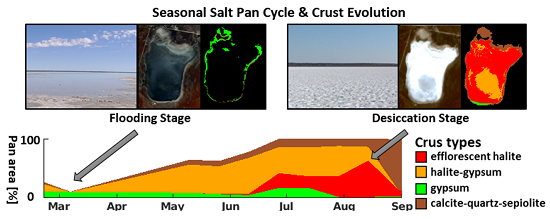
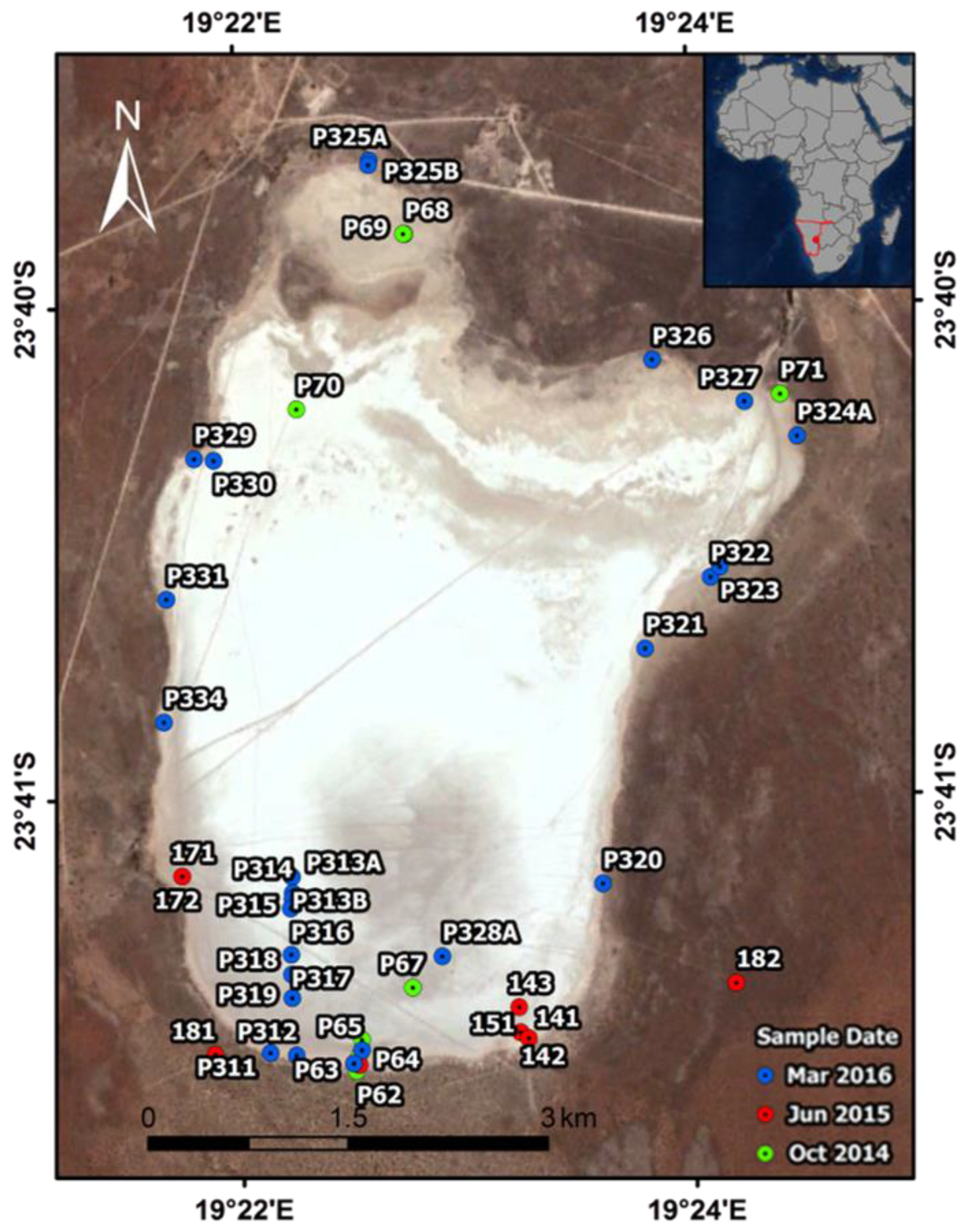
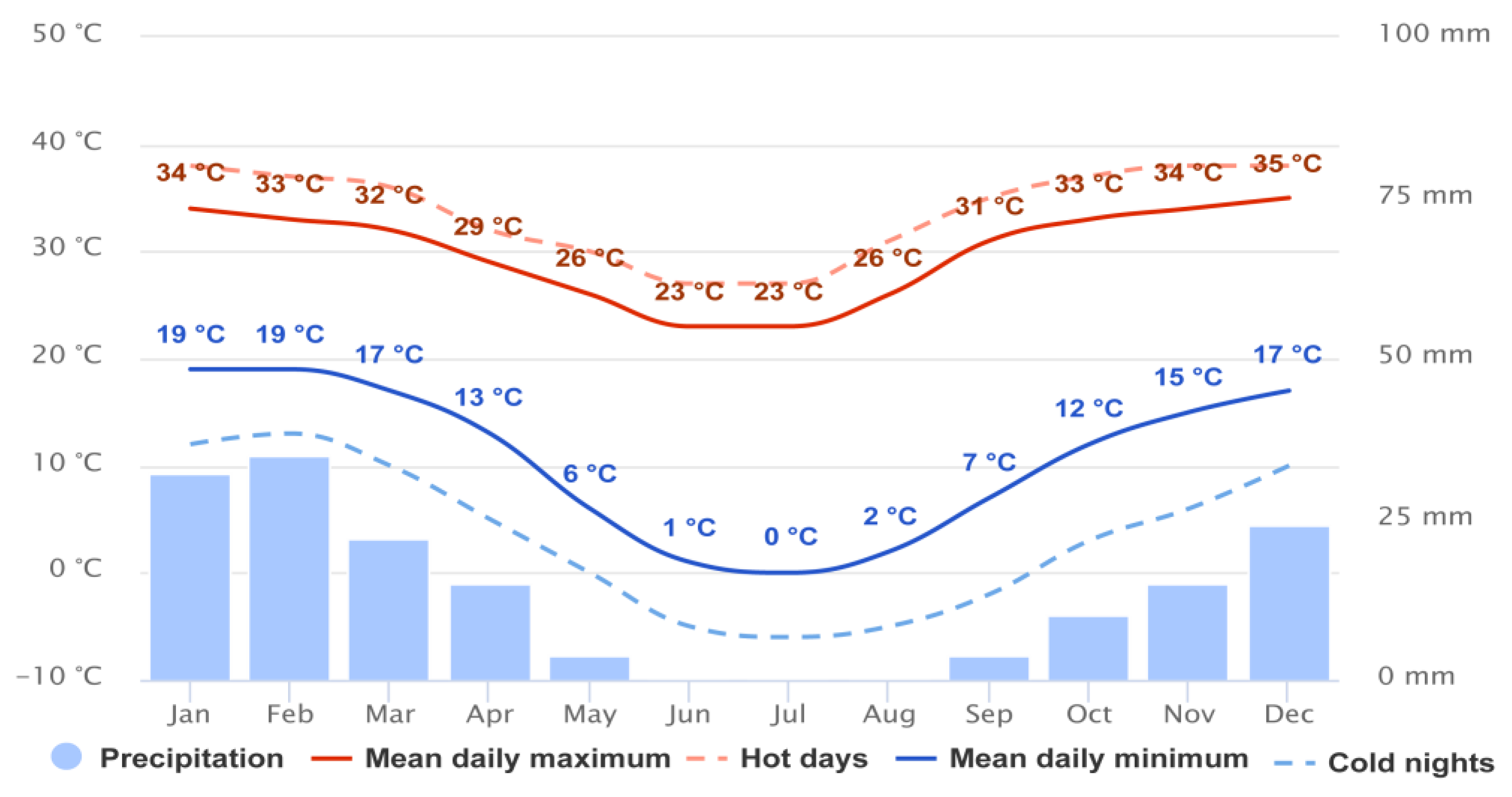
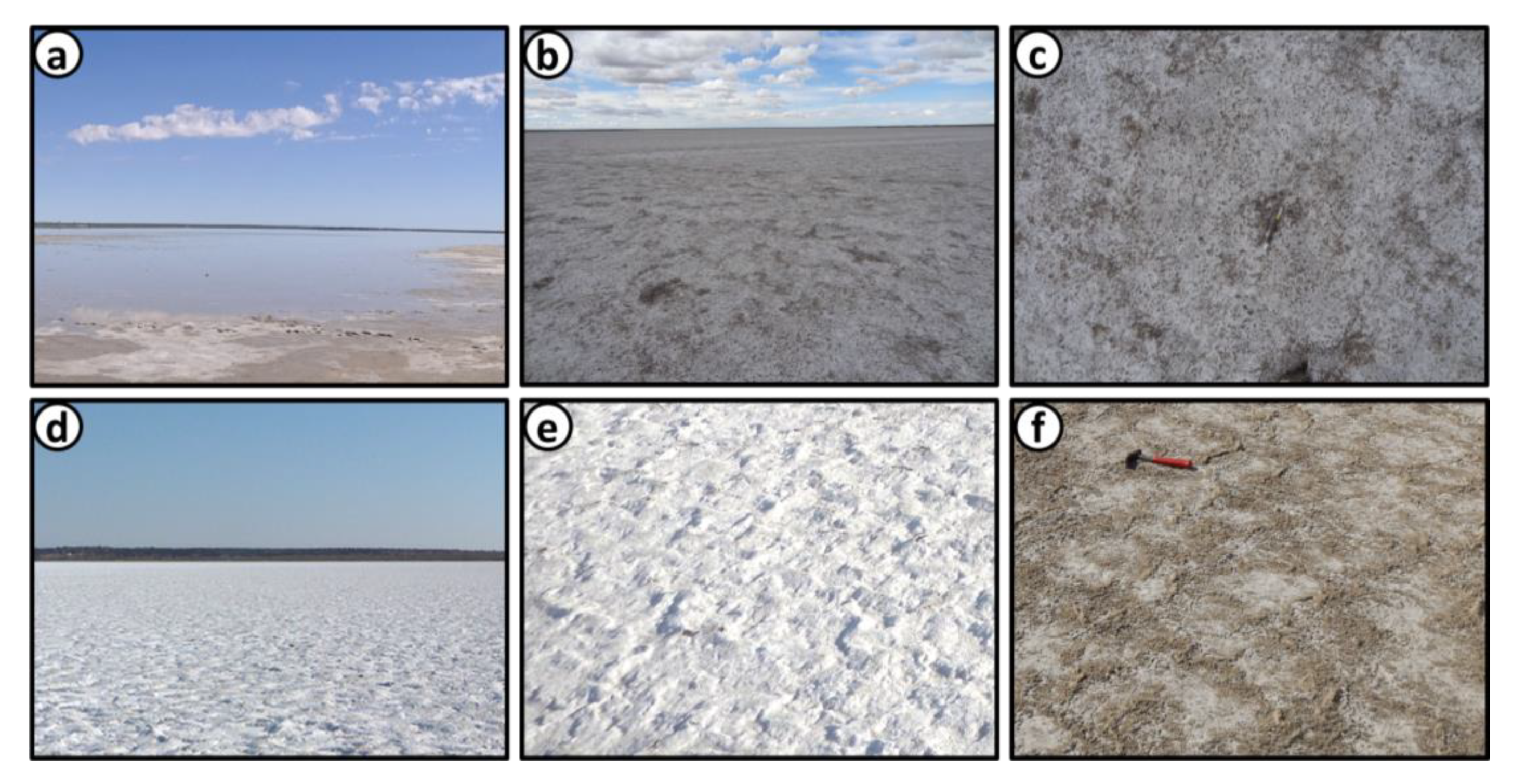
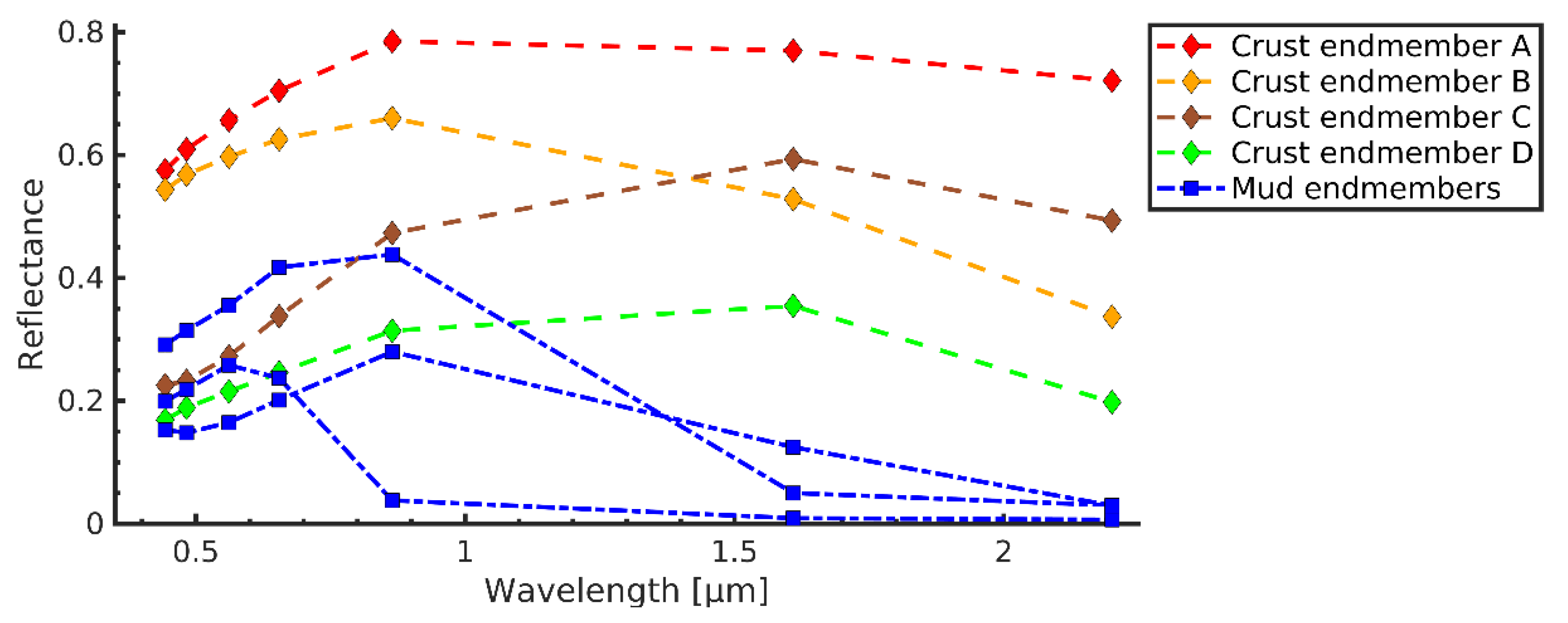
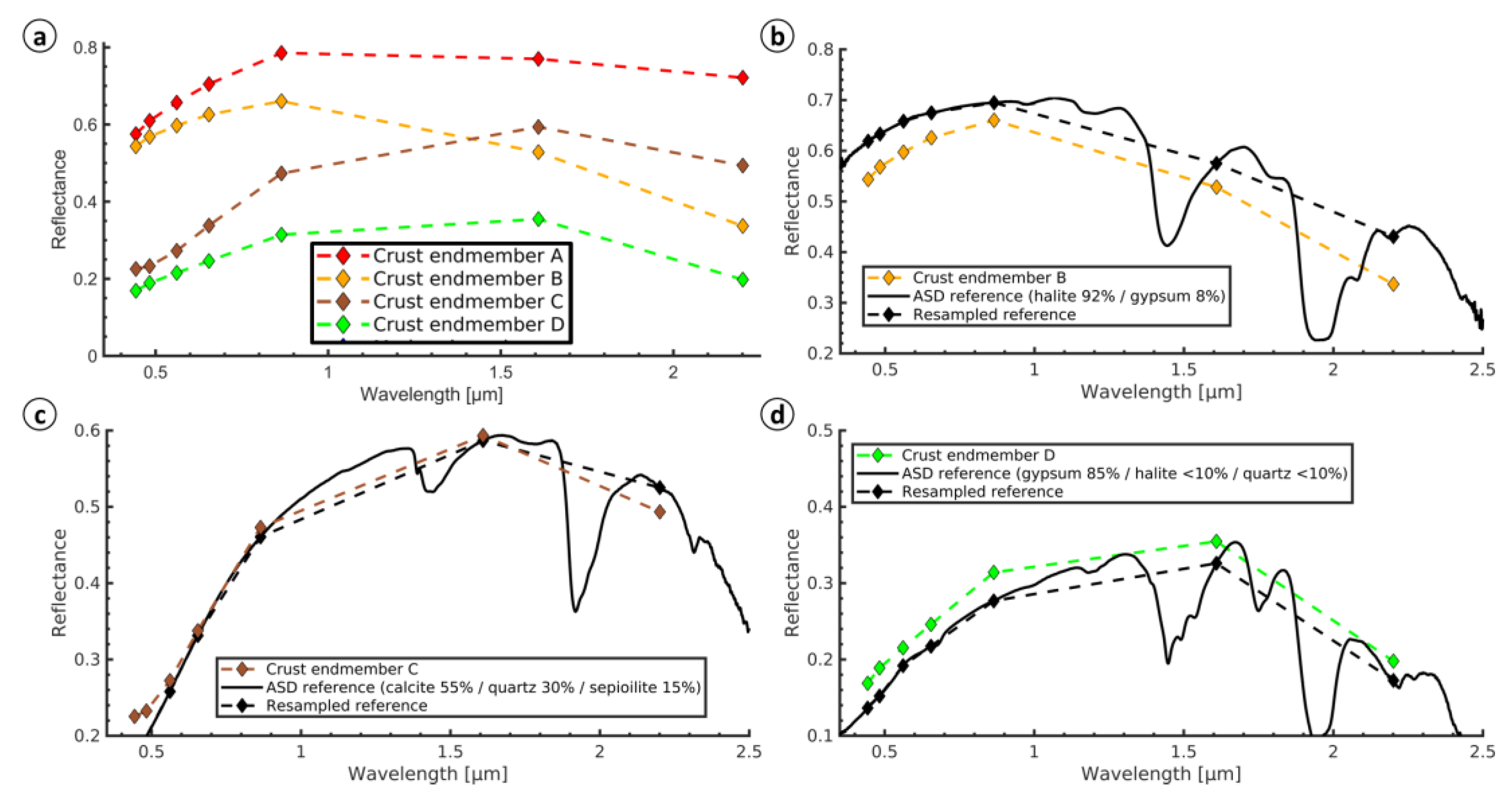
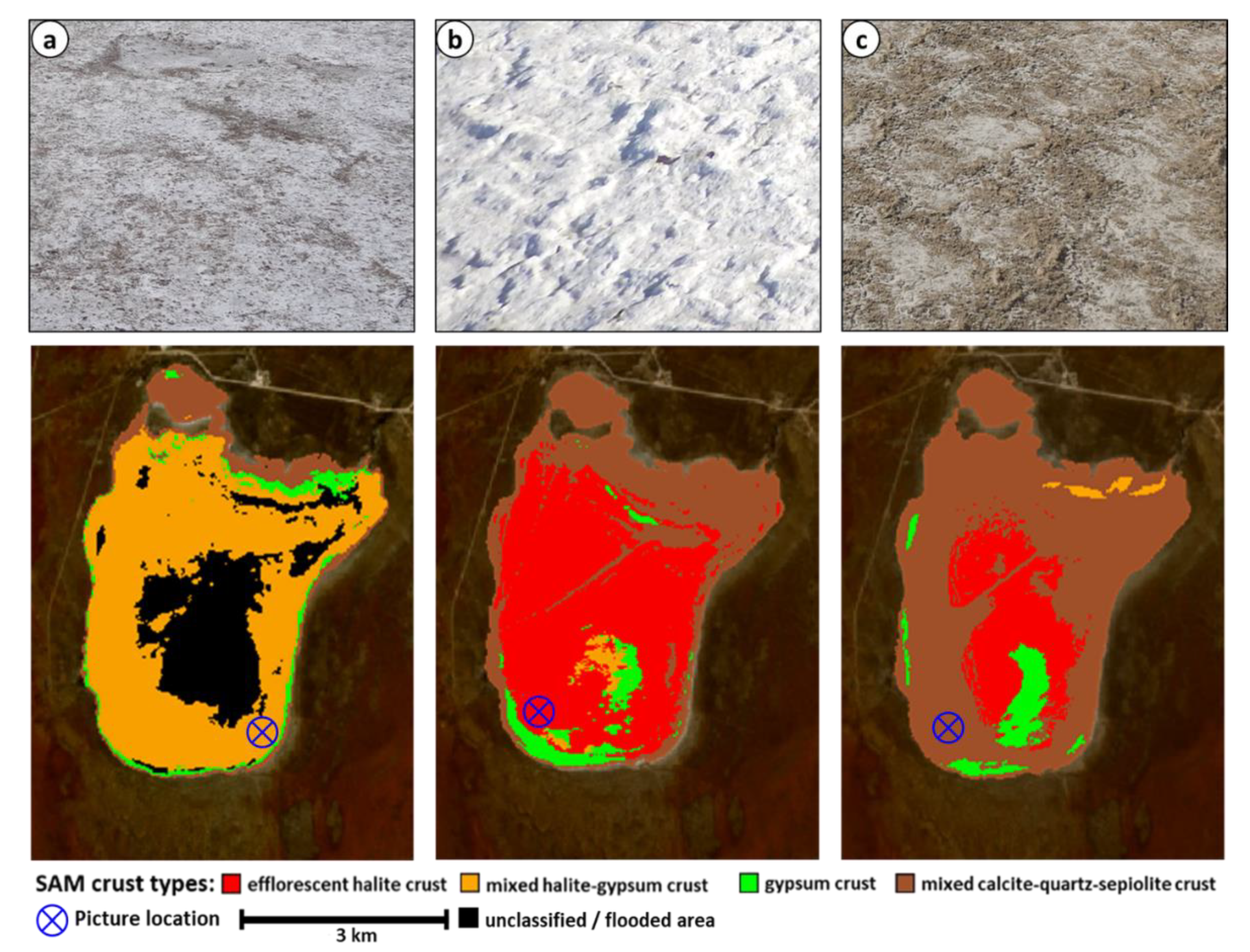
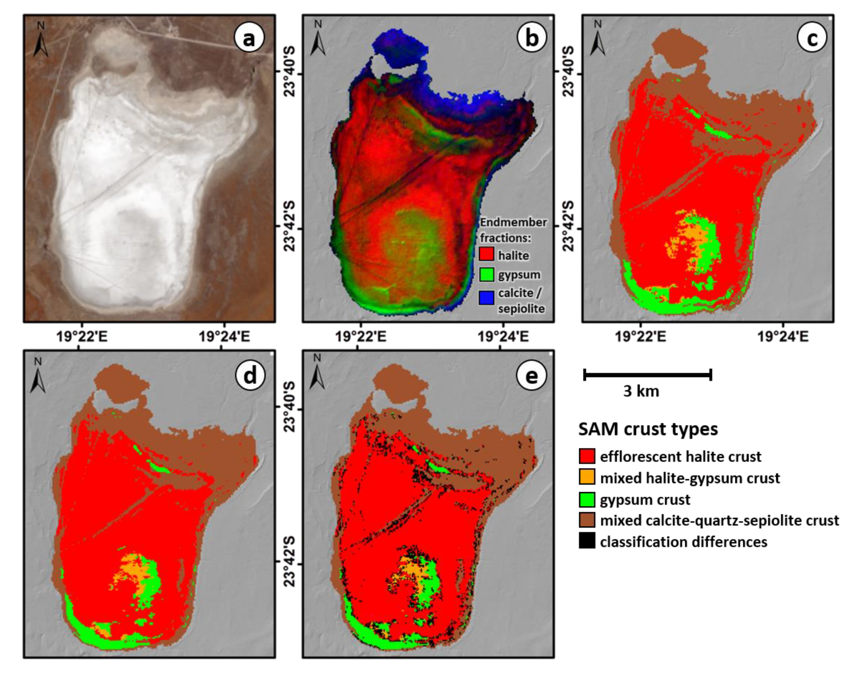
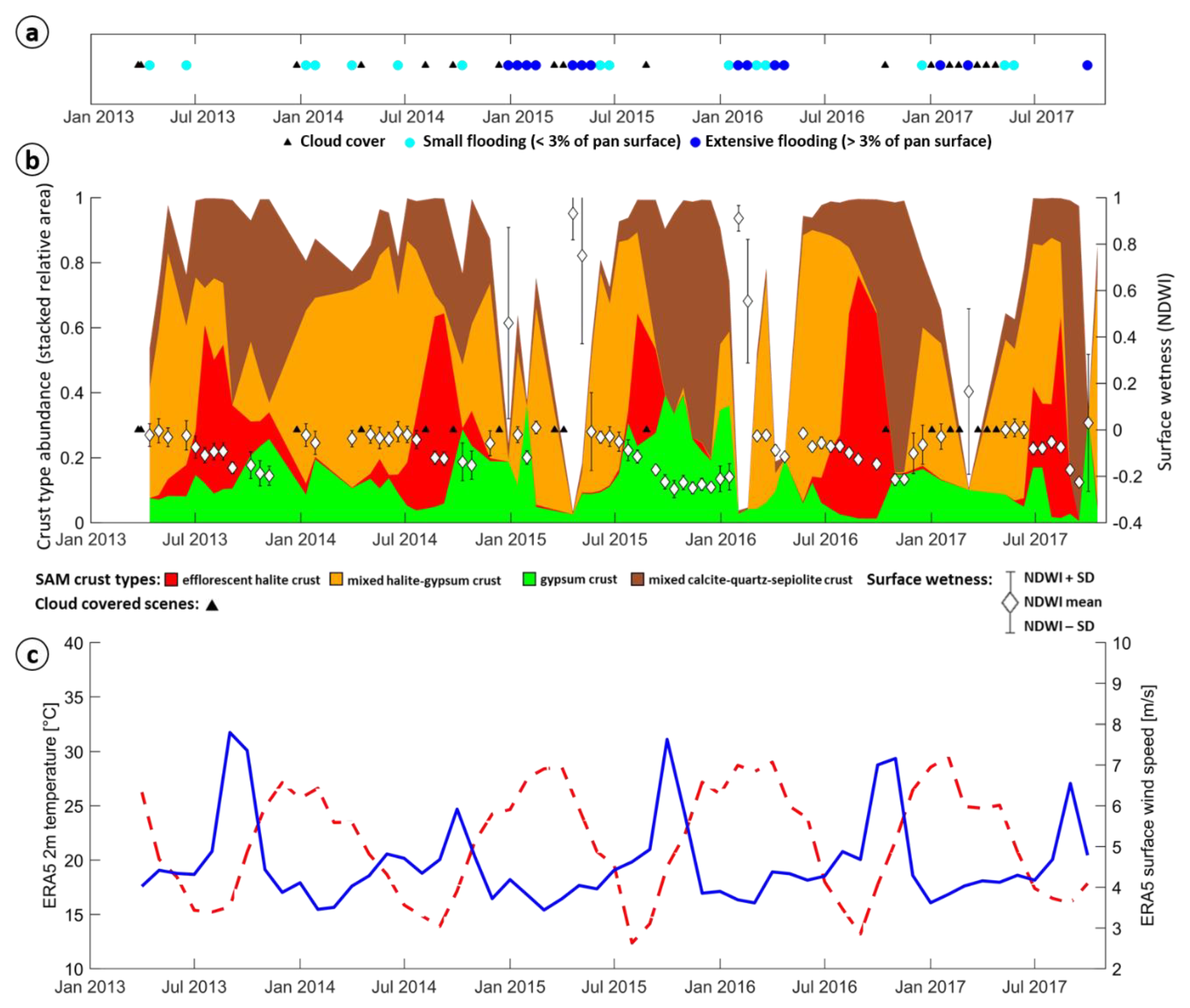
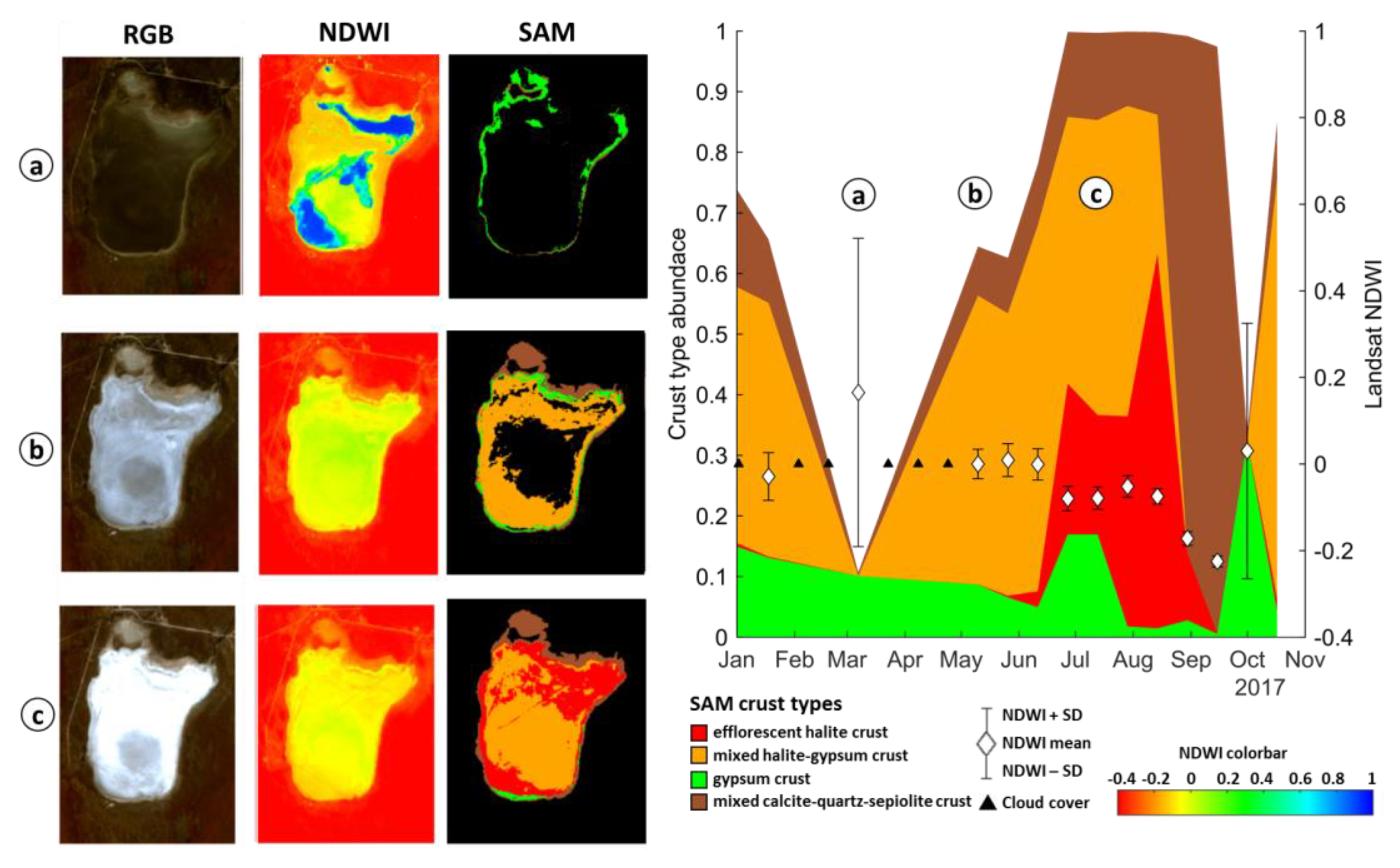
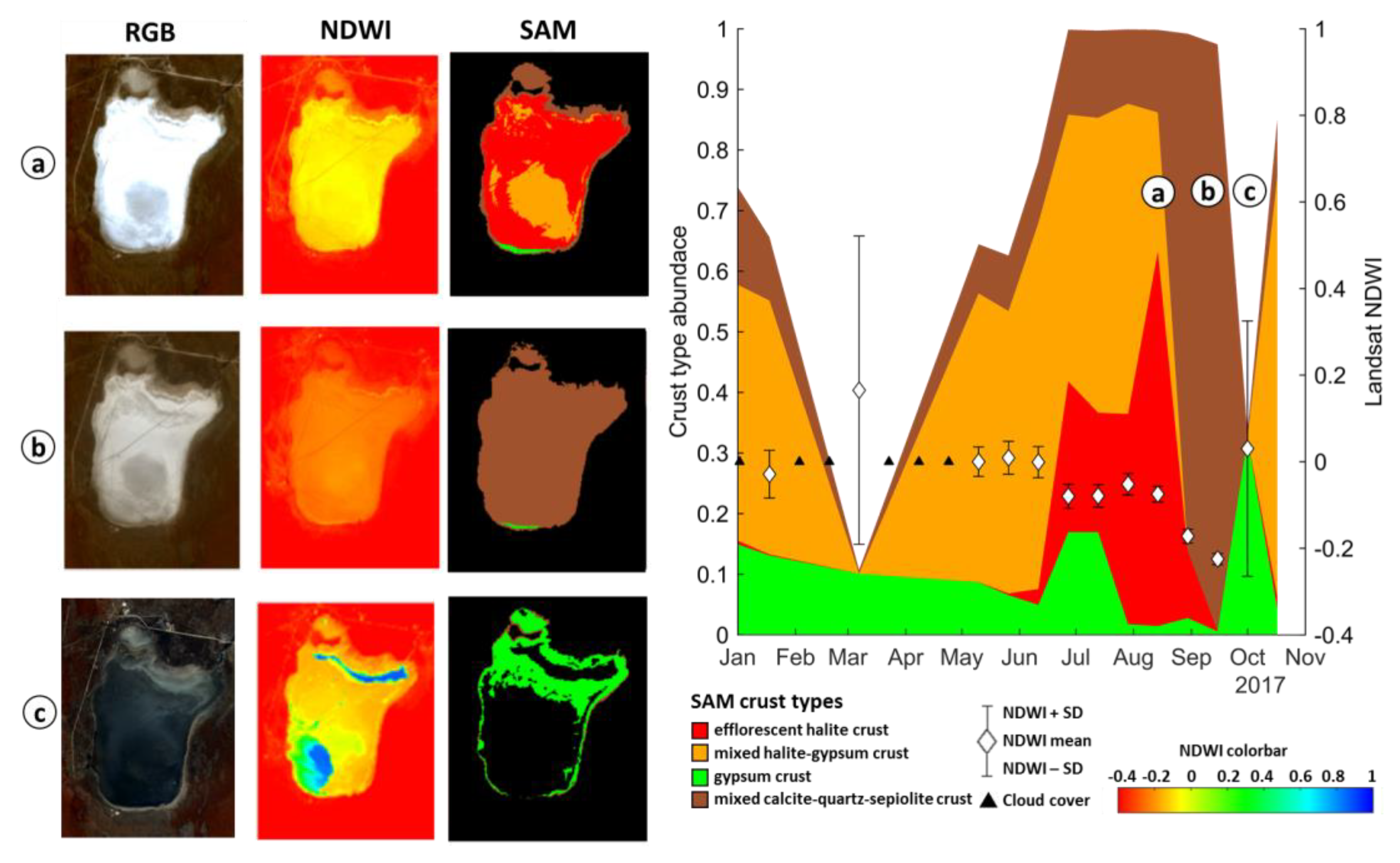
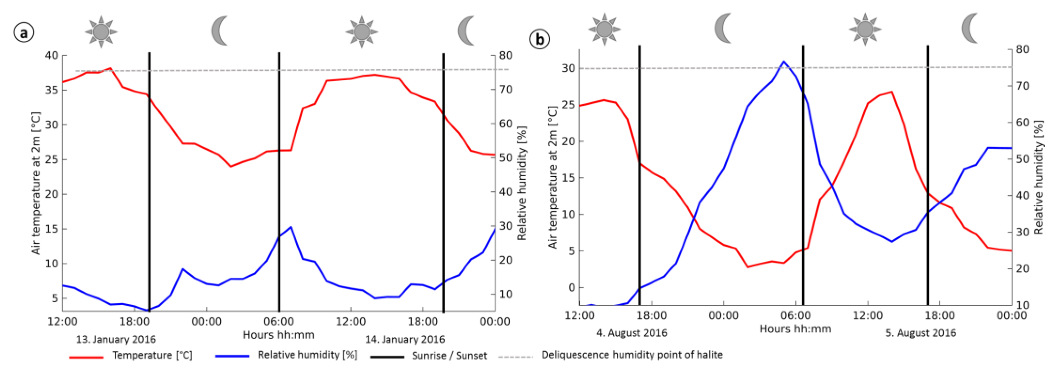
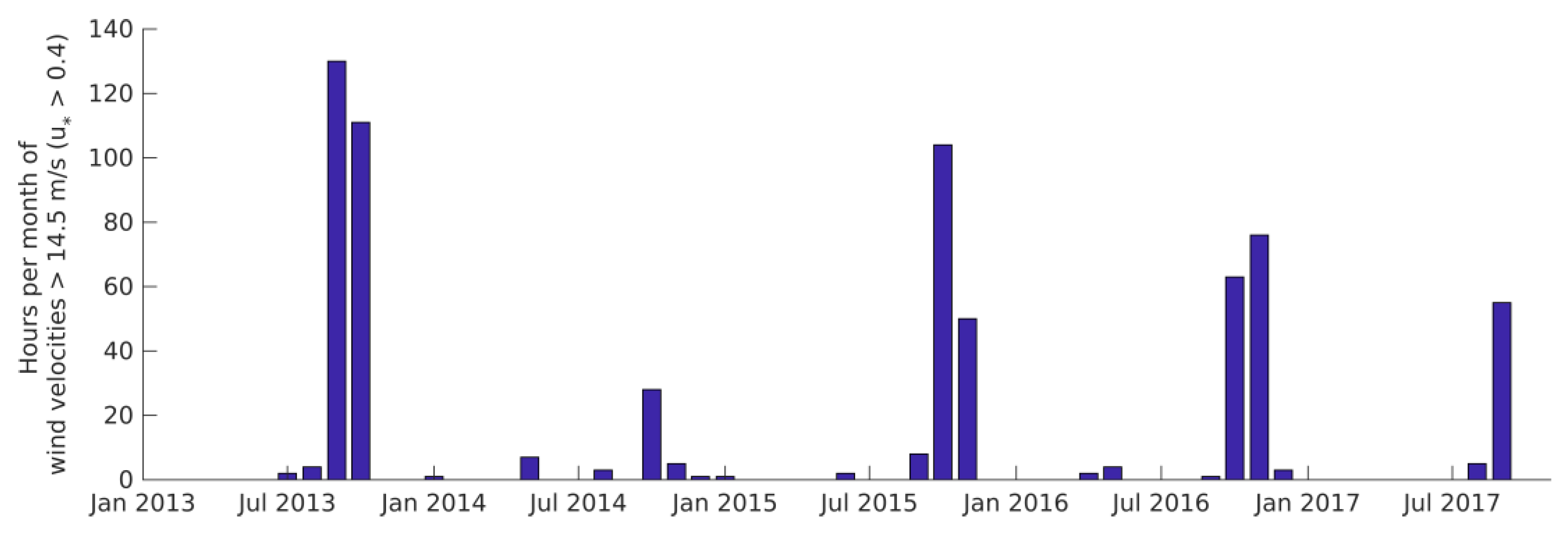
Table 1.
Confusion matrix and statistical measures for the crust of crust type mapping between Landsat Spectral Angle Mapper (SAM) classes and Hyperion-based spectral unmixing of Milewski et al. [45]: producer’s accuracy (PA), user’s accuracy (UA), overall accuracy, and Kappa coefficient.
Table 1.
Confusion matrix and statistical measures for the crust of crust type mapping between Landsat Spectral Angle Mapper (SAM) classes and Hyperion-based spectral unmixing of Milewski et al. [45]: producer’s accuracy (PA), user’s accuracy (UA), overall accuracy, and Kappa coefficient.
| Reference Data (Hyperion SAM-Based Classification) of [43] | |||||
|---|---|---|---|---|---|
| Efflorescent Halite Crust | Gypsum Crust | Mixed Halite, Gypsum Crust | Quartz, Calcite, Sepiolite Mixed Crust | UA | |
| SAM classification | |||||
| Efflorescent halite crust | 10293 (95%) | 220 (16%) | 120 (21%) | 988 (14%) | 0.87 |
| Gypsum crust | 38 (<1%) | 1004 (74%) | 39 (7%) | 38 (1%) | 0.90 |
| Mixed halite, gypsum crust | 139 (1%) | 11 (1%) | 412 (72%) | 0 (0%) | 0.73 |
| Quartz, calcite, sepiolite mixed crust | 313 (3%) | 122 (9%) | 0 (0%) | 6177 (86%) | 0.93 |
| PA | 0.96 | 0.74 | 0.72 | 0.86 | |
| Overall Accuracy | 0.90 | ||||
| Kappa | 0.82 | ||||
© 2020 by the authors. Licensee MDPI, Basel, Switzerland. This article is an open access article distributed under the terms and conditions of the Creative Commons Attribution (CC BY) license (http://creativecommons.org/licenses/by/4.0/).
Share and Cite
MDPI and ACS Style
Milewski, R.; Chabrillat, S.; Bookhagen, B. Analyses of Namibian Seasonal Salt Pan Crust Dynamics and Climatic Drivers Using Landsat 8 Time-Series and Ground Data. Remote Sens. 2020, 12, 474. https://doi.org/10.3390/rs12030474
AMA Style
Milewski R, Chabrillat S, Bookhagen B. Analyses of Namibian Seasonal Salt Pan Crust Dynamics and Climatic Drivers Using Landsat 8 Time-Series and Ground Data. Remote Sensing. 2020; 12(3):474. https://doi.org/10.3390/rs12030474
Chicago/Turabian StyleMilewski, Robert, Sabine Chabrillat, and Bodo Bookhagen. 2020. "Analyses of Namibian Seasonal Salt Pan Crust Dynamics and Climatic Drivers Using Landsat 8 Time-Series and Ground Data" Remote Sensing 12, no. 3: 474. https://doi.org/10.3390/rs12030474
Note that from the first issue of 2016, this journal uses article numbers instead of page numbers. See further details here.