An Automated Method for Surface Ice/Snow Mapping Based on Objects and Pixels from Landsat Imagery in a Mountainous Region


1
State Key Laboratory of Resources and Environmental Information System, Institute of Geographic Sciences and Natural Resources Research, Chinese Academy of Sciences, Beijing 100101, China
2
University of Chinese Academy of Sciences, Beijing 100049, China
*
Author to whom correspondence should be addressed.
Remote Sens. 2020, 12(3), 485; https://doi.org/10.3390/rs12030485
Submission received: 13 December 2019
/
Revised: 27 January 2020
/
Accepted: 30 January 2020
/
Published: 3 February 2020
Abstract
:Surface ice/snow is a vital resource and is sensitive to climate change in many parts of the world. The accurate and timely measurement of the spatial distribution of ice/snow is critical for managing water resources. Object-oriented and pixel-oriented methods often have some limitations due to the image segmentation scale, the determination of the optimal threshold and background heterogeneity. Therefore, this study proposes a method for automatically extracting large-scale surface ice/snow from Landsat series images, which takes advantage of the combination of image segmentation, the watershed algorithm and a series of ice/snow indices. We tested our novel method in three different regions in the Karakoram Mountains, and the experimental results show that the produced ice/snow map obtained a user’s accuracy greater than 90%, a producer’s accuracy greater than 97%, an overall accuracy greater than 98% and a kappa coefficient greater than 0.93. Comparing the extraction results under segmentation scales of 10, 15, 20 and 25, the user’s accuracy and producer’s accuracy from the proposed method are very similar, which indicates that the proposed method is more reliable and stable for extracting ice/snow objects than the object-oriented method. Due to the different reflectivity values in the near-infrared band in the snow and water categories, the normalized difference forest snow index (NDFSI) is suitable for Landsat TM and ETM+ images. This study can serve as a reliable, scientific reference for rapidly and accurately extracting ice/snow objects.

1. Introduction
Environmental changes and their impacts on natural ecosystems and human societies are topics of research in a wide range of scientific fields [1]. Surface ice/snow is among the most vital earth resources undergoing temporal and spatial changes as a consequence of climate change and other forms of environmental change in many parts of the world [2,3,4]. The economic, ecological and social effects of surface snow changes have been the subject of academic study for many years [5,6,7]. Furthermore, surface snow is one of the most important water resources of most rivers in high-mountain regions. It is not only the direct cause of spring flooding due to melting but also plays an important role in managing local water resources, preventing disasters, and forecasting and simulating snowmelt [8]. Due to global warming and corresponding glacier recession, ice/snow-covered areas in mountainous regions have decreased rapidly in recent decades. Therefore, monitoring and obtaining data on the dynamics of surface ice-snow in a timely manner are essential for the policy development process [9,10].
Remote sensing has become an important source of information for analyzing and delivering data on changes in various natural resources, particularly surface ice/snow [11,12]. Examples of studies using remote sensing techniques for various applications in relation to surface ice/snow resources include estimating snow-covered areas, computing the snow depth/water equivalent, mapping the regional snow cover, assessing ice/snow disasters, and hydrological and climate modeling [13,14,15,16]. Surface ice/snow has a high reflectivity in the visible and near-infrared (NIR) bands and a strong absorption in the shortwave infrared (SWIR) band, which is the theoretical basis for snow-cover mapping in optical remote sensing. Based on these characteristics, Warren (1982) first introduced the normalized difference snow index (NDSI) to delineate surface ice/snow patches using the green (band 2) and shortwave infrared (band 5) of Landsat Thematic Mapper (TM) [17]. The National Aeronautics and Space Administration (NASA), also used NDSI to produce a series of famous Moderate Resolution Imaging Spectroradiometer (MODIS) global snow products [18]. Wang (2015) proposed the normalized difference forest snow index (NDFSI) by analyzing the spectral features of snow-covered and snow-free forests, similar to the NDSI [19]. Delineating bare-ice areas based on remote sensing technology has been studied for more than 40 years. Although some practical methods—including supervised and unsupervised classification, the band ratio, and synthesis methods—have been developed to improve the overall accuracy in extracting surface ice/snow areas during this time, the NDSI still plays an important role in these methods [14,20,21].
In recent years, machine learning methods have been used to extract surface ice/snow cover in mountainous areas. He (2015) extracted snow cover in the Tianshan Mountain area based on the support vector machine (SVM) method and GF-1 images [22]. However, the experimental results indicated a mean accuracy of 83.8%, which does not have obvious advantages. Iliyana (2011) used MODIS surface reflectance, NDSI, Normalized Difference Vegetation Index (NDVI) and land cover as inputs in an artificial neural network (ANN) to extract fractional snow cover (FSC), which performed adequately, with an RMSE of 12% [16]. Elzbieta (2015) also built an ANN model to extract FSC based on 15 independent inputs, including six spectral bands from six Landsat TM/ETM+ images and terrain parameters derived from the NED DEM [23]. Although this method performed well (overall accuracy of 89%), its training input contained 98,000 pixels, which consumes a certain amount of time and manpower. Thus, compared to the NDSI and band ratio, machine learning is more complicated and has a slower calculation speed.
Imagery classification can be divided into pixel-based and object-based methods based on the classification units. The former is suitable for identifying specific targets with low spatial resolution. As the spatial resolution of remote sensing images increases, the pixel-based classification method cannot obtain good effects, which can lead to a “salt and pepper” effect in the process of extracting a specific target [24]. Conversely, object-based methods can effectively solve these problems. The image segmentation parameter is a critical factor in object-based image classification that can directly affect the accuracy of extracting a specific target. During image segmentation, over-segmentation and under-segmentation errors could occur [25]. Over-segmentation leads to the fragmentation of a specific target, while under-segmentation causes a mixed object that contains multiple land-cover classes. Therefore, selecting the optimal segmentation parameter in object-oriented classification has been a critical scientific problem [26]. In addition, the classification results of the above two methods depend highly on their classification thresholds [9,19,27,28]. Some researchers have selected the optical classification threshold based on sampling, visual effect, or frequency histogram, which limit the efficiency of extracting ice/snow [27,29].
Landsat series images have been used for a wide variety of surface ice/snow monitoring applications for more than 30 years since NASA launched the first Landsat satellite in 1972. Previous work with Landsat TM and Landsat Multispectral Scanner (MSS) has focused on the extraction of surface ice/snow areas and corresponding reflectance values [30]. Numerous studies have used either the TM or Enhanced Thematic Mapper Plus (ETM+) sensors (or, in some cases, both sensors) to create surface ice/snow-mapping for increasingly large areas after the launch of the Landsat ETM+ in 1999 [31]. Since the Landsat Operational Land Imager (OLI) launched in 2013, many scholars have paid attention to temporal and spatial changes in the surface ice/snow [32]. However, few studies have focused on the differences among Landsat series images.
In summary, some problems in the previous methods, including segmentation parameters, classification thresholds and calculation speed, still exist [16,19,23,28,29,31]. Meanwhile, there is a lack of studies comparing the differences between ice/snow indices from Landsat TM, ETM+ and OLI images. Therefore, the objectives of this study are to (1) propose a method for integrating objects and pixels to lower the impacts of segmentation parameters and classification thresholds, and (2) to compare the adaptability of the ice/snow indices in Landsat series images.
2. Study Areas and Data Sources
2.1. Study Areas
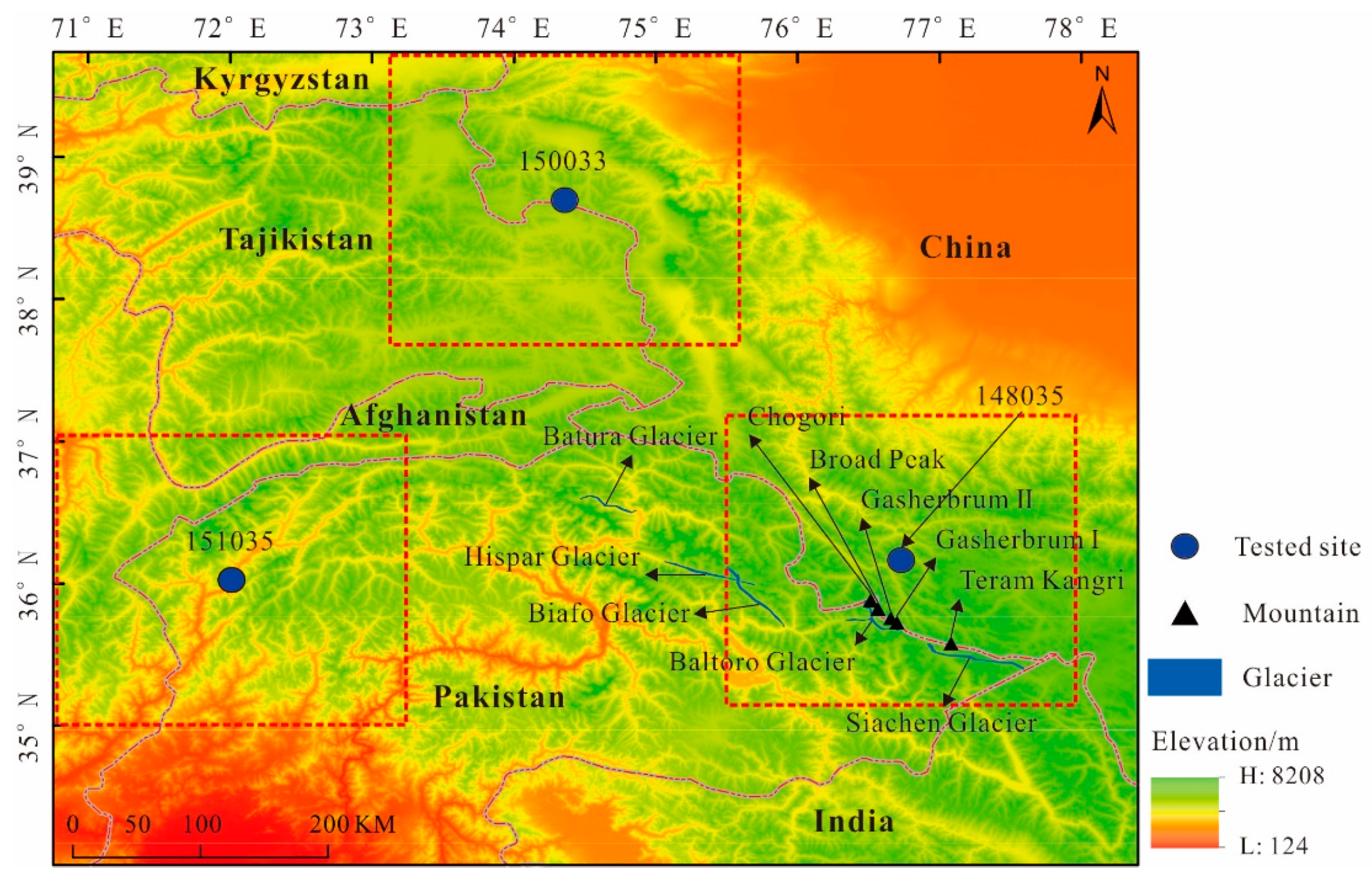
The tested sites are located at the junction of China, Kyrgyzstan, Tajikistan, Afghanistan, Pakistan and India, spanning from 71°E to 78°E and from 34°N to 40°N (Figure 1), and the Karakoram Mountains pass through this region. The Karakoram Mountains have an average elevation of over 5500 m, a length of approximately 800 km and a width of approximately 240 km, possessing five mountain glaciers (Batura Glacier, Hispar Glacier, Biafo Glacier, Baltoro Glacier and Siachen Glacier) over 50 km and five peaks over 8 km (Chogori, Broad Peak, Gasherbrum I, Gasherbrum II and Teram Kangri) [33]. They are the most concentrated place for glaciers in the world outside the Arctic region. The study area is mainly semiarid and mostly belongs to a continental climate; the southern part of the study area belongs to a humid climate due to the influence of the Indian Ocean monsoon, but the northern part is extremely dry. The annual average precipitation does not exceed 100 mm at low altitudes, but it increases in snow-covered areas at high altitudes. At an altitude of approximately 5700 m, the average temperature in the warmest month is below 0 °C in this study area.
2.2. Landsat Image
NASA has launched eight land satellites (Landsats) since 1972, and their products are widely used in various types of land and natural resource studies. Currently, only the Landsat 5, Landsat 7 and Landsat 8 products are available from the United States Geological Survey (USGS) Global Visualization Viewer (GLOVIS) portal. All the Landsat images are of product type L1T and have a scene quality score of nine, meaning perfect scenes with no detected errors. Furthermore, we selected images from August to October to obtain perennial ice/snow. Detailed descriptions of the Landsat images are shown in Table 1.
2.3. Randolph Glacier Inventory
The Randolph Glacier Inventory (RGI) is a global inventory of glacier outlines, excluding the Greenland and Antarctic ice sheets, which was compiled at several institutions and can be downloaded from the website (http://www.glims.org/RGI/) [34]. Using simple and normalized band-ratio maps, most of the ice/snow outlines in the RGI were derived from various satellite imagery, including Landsat series images, ASTER IKONOS, and SPOT 5 [35]. RGI 1.0 was first released on 22 February 2012, and has been continuously updated since then. Currently, it has been updated to RGI 6.0, released on 28 July 2017. In this study, we selected RGI 4.0 (released on 1 December 2014) and RGI 5.0 (released on 20 July 2015) to indirectly verify the experimental results. According to their revision and acquisition times, RGI 4.0 matched Image C and Image F, and RGI 5.0 matched Image I.
3. Methods
Referring to some famous classification systems, including FAO LCCS and IGBP, we regard ice and snow as the same category [36]. The overall workflow has four steps (Figure 2): (1) data preprocessing, which includes converting the digital number (DN) to top of atmosphere (TOA) reflectance data for every pixel and cloud mask, and calculating the NDSI, normalized difference forest snow index (NDFSI), normalized difference vegetation index (NDVI), NIR/SWIR and RED/SWIR; (2) applying a global threshold to extract ice/snow-covered areas after image segmentation using eCognition software (http://www.ecognition.com/suite), which is a famous remote-sensing classification tool; (3) marking ice/snow objects and building potential ice/snow-covered areas (unknown regions), and then using the watershed algorithm (https://docs.opencv.org/3.3.1/d3/db4/tutorial_py_watershed.html) to accurately delineate the boundary for each ice-snow object; and (4) evaluating the extraction results with the validation data and RGI datasets.
3.1. Data Preprocessing
The data preprocessing step includes three stages: converting the DN to the TOA reflectance, creating the cloud mask, and calculating the related indices.
The conversion of the raw pixel DN to the TOA reflectance is a basic step for Landsat image preprocessing. The DN value represents only the brightness characteristics of ground objects in the image, without any actual physical meaning. In contrast, the TOA reflectance is measured by spaceborne sensors flying outside the atmosphere, which can effectively reflect the spectral characteristics of ground objects and is widely used to calculate related indices. The conversion formula is given as follows
from which we can extract gain and offset in the header files of the Landsat series images.
Compared with other ground objects, clouds have high reflectivity in the SWIR band (2.08~2.35 µm). Based on this physical property of the Landsat images [37], we identified cloud-covered areas using single-threshold to reduce the influence of clouds on the experimental results. Furthermore, low cloudiness in the selected image also ensures the accuracy of experimental results.
Currently, the NDSI is widely used for large-scale surface ice/snow identification. The NDSI can effectively enhance the ice/snow information and suppress background information [9]. However, to some extent, using the NDSI to delineate snow-covered areas has some limitations due to heterogeneous false signals caused by the complexity of natural features. Some scholars have tried to construct a new ice/snow index according to the spectral characteristics of ice/snow in Landsat images, and introduced the NDVI and other indices to improve extraction results [27]. Although these studies can achieve good effects in their study areas, they are still limited to some extent by optical images from different sensors and different time phases. In this study, we identified snow-covered areas with different combinations of NDSI, NDFSI, NDVI, NIR/SWIR and RED/SWIR in the global extraction to obtain good extraction results (the spectral range of the SWIR band is 1.55‒1.75 µm) [14,19,31]. The expressions of these indices are as follows
where , , and represent the TOA values of the green band, red band, NIR band, and SWIR bands, respectively, for Landsat series images. Note that the spectral range for the SWIR band is 1.55‒1.75 µm.
3.2. Global Extraction Based on Objects
Object-based classification, which is an effective method for extracting specific targets from Landsat series images, can avoid the noise of pixel-based classification [38]. Before object-based classification can be performed, image segmentation is a critical step. In this study, we adopted eCognition’s multi-resolution segmentation algorithm, which is a bottom up region-merging technique starting with one-pixel objects. In numerous subsequent steps, smaller image objects are merged into bigger ones. Through this pair-wise cluster process, the weighted heterogeneity n h of the resulting image objects, where n is the size of a segment and h a parameter of heterogeneity, can be determined. In each step, that pair of adjacent image objects is merged, which results in the smallest growth exceeding the threshold defined by the scale parameter, causing the process to stop [39].
Heterogeneity in eCognition considers color and shape as primary objects. The increase in heterogeneity f has to be less than a certain threshold, which is also called a segmentation scale.
refers to difference in spectral heterogeneity, which allows multi-variant segmentation by adding a weight to the image channels c.
with number of pixels within merged object, number of pixels in object 1, number of pixels in object 2, standard deviation within object of channel c. Subscripts merge refer to the merged object, and object 1 and object 2 prior to merge, respectively.
refers to the difference in shape heterogeneity, which describes the improvement in the compactness and smoothness of an object’s shape.
l is perimeter of object, b is perimeter of object’s bounding box.
The DN values are multiples of the TOA values (the TOA values are from −1 to 1, and the DN values for Landsat TM are from 0 to 255), which makes bigger, thereby increasing and f, based on Formulas (7) and (8). Two different objects could only be merged when f is less than the segmentation scale. The increase in the heterogeneity of f could lower the probability of mixed-object and get better image segmentation results.
Therefore, the six bands (blue, green, red, nir, swir01 and swir02) from the original image were selected as the input layer to perform image segmentation using eCognition software, and then the related band ratios (NDSI, NDFSI, NDVI, NIR/SWIR, RED/SWIR) from the TOA image were applied to extract ice-snow information based on the segmentation results. We attempted to determine the segmentation scale several times, and the default values were used for and ( and ) in this study. Due to the differences between different sensors in radiation resolution, the selected segmentation scales for Landsat TM, ETM+ and OLI were 15, 15, and 150, respectively.
A large ice/snow object can be divided into several small ones by image segmentation. These small ice/snow objects could be identified with a global threshold. In this study, we used two global thresholds to delineate snow-covered areas based on the object method (Figure 2). Compared to the second global extraction, the threshold is larger in the first global extraction to ensure that the extracted ice/snow objects are accurate. The classification threshold (NDSI or NDFSI) is smaller in the second global extraction, to obtain potential snow-covered areas and provide support for building unknown regions.
Stratified random sampling was performed for different categories, and the calculations of the averages of the related indices for various categories in the study area are shown in Figure 3. According to Figure 3, there are obvious differences between the pure snow (i.e., non-shaded snow) and the other five classifications in terms of the NDFSI, NIR/SWIR and RED/SWIR for the Landsat TM and ETM+ images. However, the variances in NIR/SWIR and RED/SWIR are larger than those of the NDSI and NDFSI in pure snow sampling, as shown in Figure 3d. The NDSI has a good effect for extracting pure snow objects in Landsat OLI images. Therefore, we should extract pure snow mainly based on the NDFSI and NDSI, with NIR/SWIR and RED/SWIR as the auxiliary indices.
Ice/snow objects include two parts: pure snow and shaded snow. Compared to the pure snow type, shaded snow and water bodies have similar reflections in the five indices, which makes it difficult to directly extract shaded snow with a single criterion, as shown in Figure 3. We discovered that the differences between shaded snow and water bodies in the NDVI are larger than those in the other indices. Therefore, different criteria combinations for the five indices were applied to accurately extract ice/snow objects in this study.
We could set the classification threshold according to visual effects. Due to the differences in acquisition time and weather conditions for different images, the classification threshold varies from image to image. Taking image LE71480352002285SGS00 as an example, the criteria for the first global ice/snow extraction were as follows: (1) NDSI > 0.65, and (2) NDVI < −0.24 (Figure 4a). Based on the first global extraction results, we added a new criterion (NDSI > 0.58) for the second global ice/snow extraction (Figure 4b). The delineated boundaries of surface ice/snow in the first global extraction are more accurate than those in the second global extraction due to the strict criteria. However, there were some missing ice/snow objects in the first global extraction. Therefore, we lowered the criterion to include the potential ice/snow regions (also called unknown regions) and readjusted their boundaries in the local extraction based on pixels.
3.3. Local Extraction Based on Pixels
The object-based method regards the object as the basic classification unit, but the pixel-based method regards the pixel as the basic classification unit, which is their essential difference [24,25]. The delineated boundaries of surface ice/snow do not meet the mapping requirements, even after global extraction. Therefore, we needed to extract the unidentified ice/snow pixels from background information in the pixel layer.
As shown in Figure 4, the first depicted ice/snow areas are smaller than the actual ice/snow areas, while the secondary depicted ice/snow areas may be mixed with non-ice/non-snow pixels. To shrink the gaps between the automatically extracted ice/snow boundaries and the actual ice/snow boundaries, all the ice/snow bodies that were extracted in the first global extraction were numbered from 1 to n. Then, using the watershed algorithm, the boundary of every ice/snow body was readjusted within its potential ice/snow region.
The watershed algorithm regards the gradient image as a topographic surface and then floods from the minima based on region growing [40,41]. Finally, the image can be divided into watershed lines and catchment basins. Although the watershed algorithm has obvious advantages in terms of effectiveness and weak edge detection, over-segmentation cannot be avoided due to image noise. Therefore, a marker extraction method for the watershed algorithm was proposed [42,43]. The extracted ice/snow markers, representing the interior of different ice/snow bodies, are regarded as the minima of gray images and suppress all other gradient minima.
In the process of local extraction, we first numbered the depicted ice/snow bodies in the first global extraction, which were regarded as the sure foreground for the watershed algorithm (Figure 5a). The sure foreground, encircling a non-snow body, is segmented into multiple ice/snow bodies to ensure that the watershed algorithm works. Therefore, the segmented ice/snow objects need to be re-marked (Figure 5b). Next, the buffer regions produced by the second global extraction results were spatially overlaid with the segmented ice/snow objects to develop the final markers (Figure 5c). The final markers include the sure ice/snow and unknown regions. Finally, based on the watershed algorithm, the boundary of every ice/snow object was automatedly modified within its unknown regions. The final extraction effect of ice/snow is shown in Figure 5d.
3.4. Accuracy Assessment
In this study, we adopted two methods for validating the experimental results from the qualitative and quantitative perspective. On the one hand, the extraction results and the RGI datasets were used to describe the boundaries of ice–snow from actual images and to show whether our method is effective from a qualitative perspective.
On the other hand, modifying the first global extraction results by visual interpretation were regarded as validation data (Figure 2). We counted the corrected number of ice/snow pixels a, the commission number of ice/snow pixels b, the omission number of ice/snow pixels c and the corrected number of non-ice/snow pixels d. Six traditional indicators were selected—user’s accuracy (UA), producer’s accuracy (PA), commission error (CE), omission error (OE), overall accuracy (OA) and kappa coefficient from the confusion matrix [44], to evaluate the differences between the experimental results and the actual ice/snow boundaries for every image scene. The formulas of partial indicators are as follows
4. Results
4.1. Surface Ice/Snow Areas Mapped Using Different Images
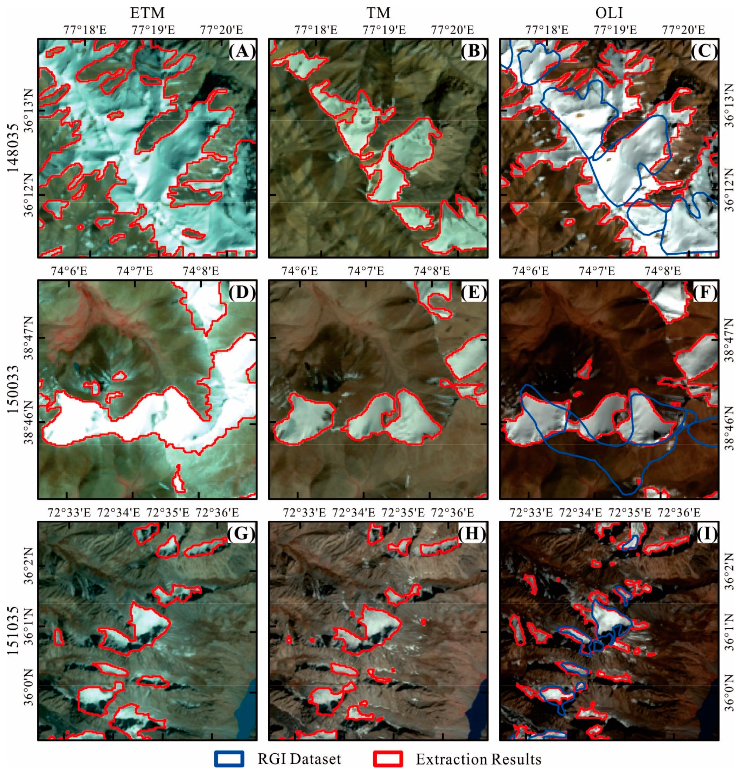
The developed method was implemented to identify the boundaries of surface ice/snow in the nine image scenes, as shown in Figure 6. We can see that the delineated boundaries of ice/snow from the developed method fit perfectly with the actual boundaries for different regions and time phases in this figure. Some weak boundaries were also effectively identified, and only a few ice–snow objects were missing. Although there were many shaded snow-covered areas in three images from region: 151035, they were still delineated with the proposed method.
Compared to the delineated boundaries from the proposed method, the depicted boundaries from the RGI datasets did not cover the snow area well. Although the snow-covered areas from the RGI datasets were reflected in the OLI images, there were some obvious omission errors and commission errors for snow. Moreover, the corrected areas from the RGI datasets were significantly less than the misclassified areas in Image F. From a qualitative perspective, the proposed method can meet the requirements of ice/snow mapping.
4.2. Accuracy Assessment of the Extraction Results
To validate the extracted results for surface ice/snow, we modified the first global extraction results, converted them from vector to raster data, recorded the differences between the two results for each pixel and constructed a confusion matrix. A relatively straightforward comparison is shown in Table 2. Generally, large kappa coefficients (more than 0.93) and a large overall accuracy (greater than 98%) can be observed, which shows that there is great consistency between the experimental results and the reference results.
For the ice/snow category, the user’s accuracies ranged from 89.55% to 96.13%, and the mean accuracy was 93.70%; the producer’s accuracies ranged from 98.01% to 99.26%, and the mean accuracy was 98.77%. These data intuitively show that the proposed method is suitable for extracting snow-covered areas. There is an interesting phenomenon that the user’s accuracies are all lower than the producer’s accuracies, which is mainly induced by some non-snow pixels that are misclassified as snow pixels. A global threshold was selected as a criterion for distinguishing ice/snow pixels from non-snow pixels during object-based global extraction. Although we used different combinations of the NDSI, NDFSI, NDVI, NIR/SWIR and RED/SWIR for different images to improve the global extraction results in this study, there were still some non-snow objects that were misidentified as ice/snow objects. The ice/snow pixels in unknown regions were extracted with the watershed algorithm to readjust the boundaries of the ice/snow objects during pixel-based local extraction, which reduced the omission error and improved the producer’s accuracy for the ice/snow category. Moreover, it is demonstrated that the watershed algorithm has a good response to weak edges.
For the non-snow category, the user accuracies and producer accuracies are all higher than 97.9%, which is mainly because the non-snow-covered areas are larger than the ice/snow-covered areas in each image scene. Taking Image A as an example, the number of non-snow pixels (39,558,086) is greater than that of snow pixels (15,893,225) according to Table 3, which makes the user’s and producer’s accuracies of non-snow greater than 98%. Compared to the non-snow category, the user’s and producer’s accuracies of snow have obvious differences, due to the smaller covered areas, which is consistent with Zhao’s research [45]. The number of omission pixels is only one-sixth of the commission pixels in Table 3, which indicates that the watershed algorithm can effectively identify ice/snow pixels from unknown regions in local extraction to improve the total accuracy.
5. Discussion
5.1. The Influence of the Segmentation Scale on the Extracted Results
Image segmentation is a key step in the analysis of remote sensing imagery. The scale parameter is directly related to the quality and accuracy of object-oriented analysis in the segmentation process [26]. Selecting an inappropriate segmentation scale may cause mixed objects to merge or may fragment the ground objects, thereby decreasing the accuracy of the information extraction. Therefore, some researchers have quantified the difference between the actual segmentation results and the reference results with the potential segmentation error and Euclidean distance to evaluate the image segmentation results in a supervised manner [46,47]. They have also calculated the homogeneity within each ground object to evaluate it in an unsupervised manner [48]. However, the abovementioned methods are time consuming and labor intensive to implement, which is not suitable for large-scale mapping.
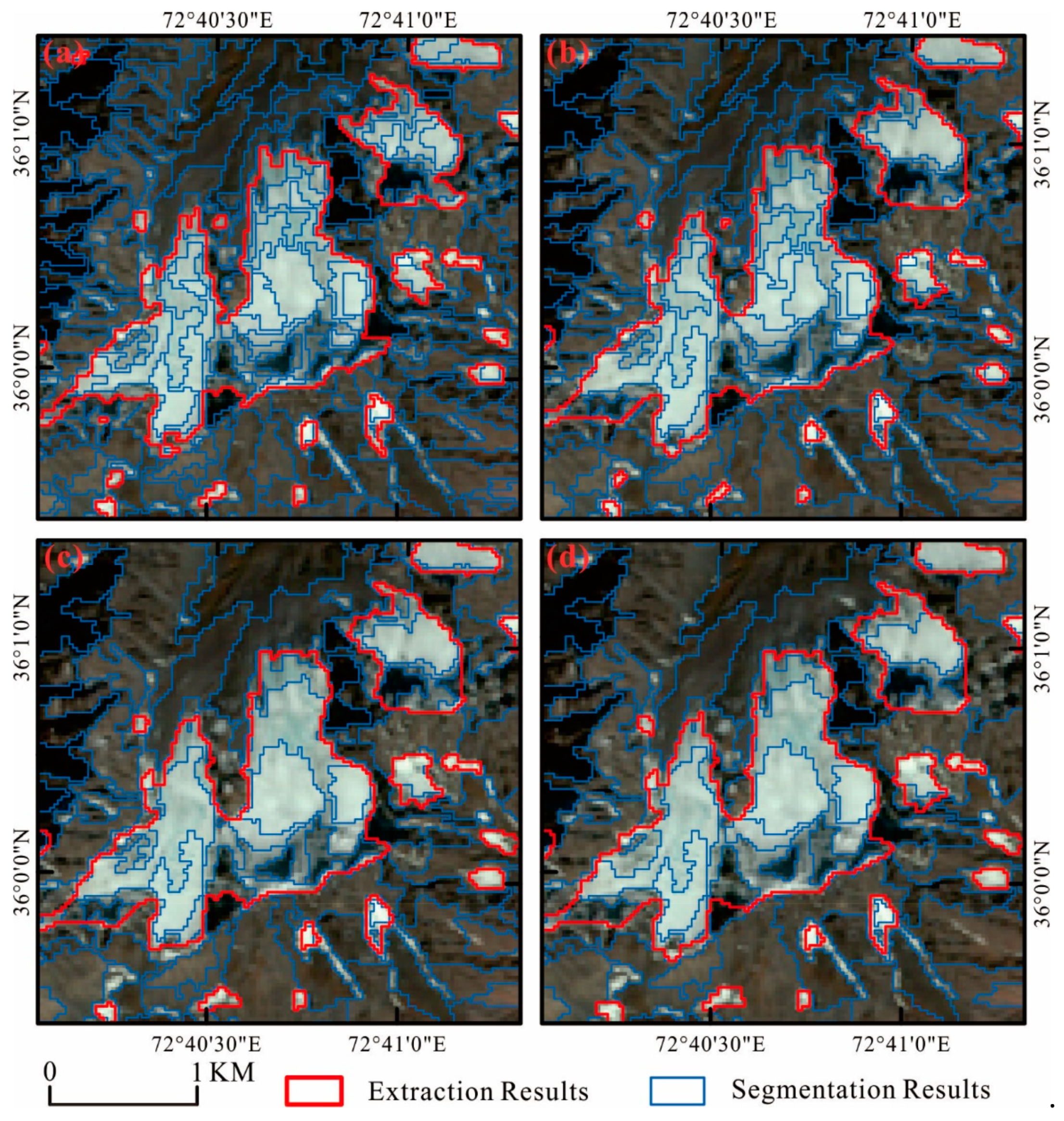
In this study, we determined the scale parameter based on visual effects to carry out image segmentation with eCognition in the global extraction phase. This method may not obtain an absolute optimal segmentation parameter, but it does not require sample-based image analysis and has high efficiency. Moreover, the boundaries of the ice/snow objects were readjusted with the watershed algorithm, which can eliminate the influence of the segmentation scale on the extraction results to some extent. As shown in Figure 7, Image H was segmented with different scales (10, 15, 20 and 25). The depicted boundaries under different segmentation scales are very similar for large ice/snow objects, and there are some gaps between the extraction results under different segmentation scales for small ice/snow objects. Some very small ice/snow objects are missed within a large segmentation scale because they will be mixed with other backgrounds. In other words, although there are different image segmentation effects under different scale parameters, the delineated boundaries for those are very similar.
According to Figure 8, the UA and PA of the proposed method (TPM) and the object-oriented method (TOM) change substantially when the segmentation scale varies from 25 to 200, illustrating that, regardless of the chosen method, the classification accuracy is affected by the segmentation scale. However, when the segmentation scale is less than or equal to 25, the user’s accuracy, producer’s accuracy, commission error, and omission error of TPM are obviously smaller than those of TOM. Under these scales (10, 15, 20 and 25), the maximum differences in the user’s and producer’s accuracies based on TPM are only 1.56 and 0.31, respectively; those based on TOM are 6.12 and 7.52, respectively. The results show that the extraction results from TOM are more dependent on imagery segmentation. Compared to TOM, TPM adds the local extraction based on the watershed algorithm, which readjusts the boundaries of ice and snow areas, thereby shrinking the gaps between the different extraction results within a certain segmentation scale.
For the ice/snow category, UA and PA of TPM are all higher than those of TOM, as shown in Figure 8. The average UA of TPM is 92.23% under these scales (10, 15, 20 and 25), but that of TOM is 87.90%. Similarly, the average PA of TPM is 97.94% under these scales (10, 15, 20 and 25), but that of TOM is 87.34%. The UA is similar for PA using TOM, and TPM has more obvious effects in improving PA than UA. This is mainly because TPM could reduce the omission number of ice/snow pixels c and increase the corrected number of ice/snow pixels a. Therefore, we can conclude that the proposed method can not only improve the extraction results, but also lower the impacts of segmentation scale to some extent.
5.2. The Influence of the Classification Threshold on the Extracted Results
The classification threshold is another important factor in remote sensing analysis. Using a relatively small threshold will increase the commission error, but using a relatively large threshold will increase the omission error. Therefore, selecting an optimal threshold is still a challenging task. Currently, researchers mainly extract the optimal threshold by sampling-based image analysis and expert experience [29,49]. However, it is difficult to distinguish ice/snow from the background effectively by using a simple threshold.
In this study, we used a relatively large NDSI or NDFSI value to extract pure ice/snow objects in the first global extraction, which could decrease the commission error but also increase the omission error. Then, based on the watershed algorithm, the total classification threshold for each ice/snow object was modified to readjust its boundary within its unknown region, which makes the classification threshold dynamic for each ice/snow object and decreases the omission error. As shown in Table 2, the omission errors for the ice/snow category are very small, ranging from 0.74% to 1.99%. Moreover, according to Figure 8, the omission errors of the proposed method are significantly fewer than those of the object-oriented method. These assessment results illustrate that the proposed method can effectively reduce the omission error and improve the overall accuracy.
There are also some similar “global-local” approaches for extracting specific ground objects [45]. The unknown regions are usually buffer zones directly produced by pure regions of a specific target, which can easily cause an increase in the commission error or omission error. As shown in Figure 4a, if the unknown regions were directly produced by ice/snow objects from the first global extraction, then the omission error would be obviously increased, thus reducing the overall accuracy. Compared to the traditional method, the unknown regions comprise two parts in the proposed method: (1) buffer zones produced by ice/snow objects from the first and second global extractions and (2) ice/snow objects from the second global extractions. The expanding method for unknown regions is more targeted, to reduce missed ice/snow objects and improve the overall accuracy.
Generally, the classification threshold has a great impact on the extraction results of the traditional method [29,50], which requires calculating the optical threshold to reduce the commission and omission errors. However, it is difficult to obtain the optimal classification threshold. A series of sampling-based image analyses may be necessary. Compared to the traditional method, there is no strict criterion for the optimal classification threshold in the proposed method, which is simple and effective. The classification threshold for each ice/snow object would be modified within its unknown region to meet its actual boundary. Therefore, the proposed method can decrease the impact of the classification threshold on the extraction results to some extent.
5.3. NDSI based on Landsat TM, ETM+ and OLI
Landsat images have been the most widely used data source for ice/snow mapping in recent decades, due to their long time series and high spatial resolution, although other images, including MODIS, Sentinel and SPOT5, have also been employed to map surface ice/snow [16,17,22,29]; the NDSI has also played an important role in this task. However, few studies have been conducted to compare the different responses of the NDSI to Landsat TM, ETM+ and OLI.
For Landsat TM and ETM+ images, ice/snow has a high reflectivity in the visible and NIR bands and has an absorption in the SWIR band [14,51]. The water body has similar spectral properties in the visible and SWIR bands, resulting in a similar reflectivity value for ice/snow and water bodies in the NDSI [27]. However, water bodies have a low reflectivity in the NIR band, which illustrates that the reflectivity of ice/snow is higher than that of water bodies in the NDFSI. As shown in Figure 3a,c, the NDSI makes no clear distinction between snow and water bodies. However, there is an obvious difference between them in terms of NDFSI. Therefore, the extraction results with the NDFSI are better than those with the NDSI in the Landsat TM and ETM+ images for the ice/snow category.
According to Figure 3b, the reflectivity of the NDSI in the Landsat OLI image has an obvious difference between the snow and water bodies, which is different from the Landsat TM and ETM+ images. Comparing these three sensors, we can discover that the spectral resolution from the Landsat OLI image is higher than that from the Landsat TM and ETM+ images, as shown in Table 4. The SWIR bandwidth (swir01) from Landsat OLI is only 0.1 µm, but those of Landsat TM and ETM+ are 0.2 µm. We can capture the subtle differences between different ground objects by improving the spectral resolution. In addition, the radiation resolution is increased from 8 bits to 16 bits, which enhances the contrast between different ground objects [9]. These changes produce obvious differences between surface ice/snow and water bodies in the NDSI from Landsat OLI images. Therefore, extracting ice/snow with the NDSI is suitable when using Landsat OLI images.
6. Conclusions
In the context of global warming, there is an urgent need to monitor earth surface ice/snow with Landsat series images in a timely and automatic manner. However, the accurate and rapid extraction of ice/snow in mountainous regions is still a challenging task due to many factors, such as image noise, image segmentation scale, classification criteria, mountain shadows and water bodies. Based on these challenges, a new method, that combines object-oriented classification and the watershed algorithm, was designed in this study to delineate the boundaries of ice/snow objects from Landsat TM, ETM+ and OLI images. The quantitative assessment of the extraction results by constructing a confusion matrix shows that the produced ice/snow map obtained a producer’s accuracy greater than 97%, an overall accuracy greater than 98% and a kappa coefficient greater than 0.93. These results indicate that the developed method can obtain a good effect in extracting ice/snow objects in the mountainous region.
Comparing the extraction results under different segmentation scales and analyzing the impacts of the classification threshold, we discover that the proposed method is more stable and reliable for delineating the boundaries of ice/snow compared to the object-oriented method. This method, based on objects and pixels, can be used not only to extract ice/snow, but also to extract water bodies and other single objects, and it has broad applicability. Furthermore, due to the differences in the spectral and radiation resolutions, different indices and their combinations should be applied during global extraction when using Landsat series images.
Author Contributions
X.W. drafted the manuscript and was responsible for data preparation, experiment, and analysis. X.G. participated in data collection. X.Z. was responsible for the research design and analysis, designed and reviewed the manuscript. W.W. and F.Y. validated the experimental results. All authors contributed to the editing and reviewing of the manuscript. All authors have read and agreed to the published version of the manuscript.
Funding
This research was funded by the Strategic Priority Research Program (Class A) of the Chinese Academy of Sciences grant number XDA23090503, and National Key Research and Development Plan of China grant number YS2018YFGH000001.
Acknowledgments
We wish to thank the editor of this journal and the anonymous reviewers during the revision process.
Conflicts of Interest
The authors declare no conflict of interest.
References
- Feyisa, G.L.; Meilby, H.; Fensholt, R.; Proud, S.R. Automated Water Extraction Index: A New Technique for Surface Water Mapping Using Landsat Imagery. J. Remote Sens. Environ. 2014, 140, 23–35. [Google Scholar] [CrossRef]
- Wekerle, C.; Colleoni, F.; Näslund, J.O.; Brandefelt, J.; Masina, S. Numerical reconstructions of the penultimate glacial maximum Northern Hemisphere ice sheets: Sensitivity to climate forcing and model parameters. J. Glaciol. 2016, 62, 607–622. [Google Scholar] [CrossRef] [Green Version]
- Erokhina, O.; Rogozhina, I.; Prange, M.; Bakker, P.; Bernales, J.; Paul, A.; Schulz, M. Dependence of slope lapse rate over the Greenland ice sheet on background climate. J. Glaciol. 2017, 63, 568–572. [Google Scholar] [CrossRef] [Green Version]
- Belart, J.C.; Magnusson, E.; Berthier, E.; Pálsson, F.; Adalgeirsdottir, G.; Jóhannesson, T. The geodetic mass balance of Eyjafjallajökull ice cap for 1945–2014: Processing guidelines and relation to climate. J. Glaciol. 2019, 65, 395–409. [Google Scholar] [CrossRef] [Green Version]
- Tilburg, C.V.; Grissom, C.K.; Zafren, K.; Mclntosh, S.; Radwin, M.I.; Paal, P.; Haegeli, P.; Smith, W.W.; Wheeler, A.R.; Weber, D.; et al. Wilderness Medical Society practice guidelines for prevention and management of avalanche and nonavalanche snow burial accidents. J. Wildern. Environ. Med. 2017, 28, 23–42. [Google Scholar] [CrossRef] [Green Version]
- Gavazov, K.; Ingrisch, J.; Hasibeder, R.; Mills, R.T.; Buttler, A.; Gleixner, G.; Punpanen, J.; Bahn, M. Winter ecology of a subalpine grassland: Effects of snow removal on soil respiration, microbial structure and function. J. Sci. Total Environ. 2017, 590, 316–324. [Google Scholar] [CrossRef]
- Moreno-Gené, J.; Sánchez-Pulido, L.; Cristobal-Fransi, E.; Daries, N. The economic sustainability of snow tourism: The case of ski resorts in Austria, France, and Italy. J. Sustain. 2018, 10, 12. [Google Scholar] [CrossRef] [Green Version]
- Fountain, A.G.; Glenn, B.; Scambos, T.A. The changing extent of the glaciers along the western Ross Sea, Antarctica. J. Geol. 2017, 45, 1–4. [Google Scholar] [CrossRef]
- Fahnestock, M.; Scambos, T.; Moon, T.; Gardner, A.; Haran, T.; Klinger, M. Rapid large-area mapping of ice flow using Landsat 8. J. Remote Sens. Environ. 2016, 185, 84–94. [Google Scholar] [CrossRef] [Green Version]
- Yumashey, D.; Hope, C.; Schaefer, K.; Riemann-Campe, K.; Iglesias-Suarea, F.; Jafaroy, E.; Whiteman, G.; Young, P. Climate policy implications of nonlinear decline of Arctic land permafrost and other cryosphere elements. J. Nat. Commun. 2019, 10, 1900. [Google Scholar] [CrossRef] [Green Version]
- Dozier, J.; Green, R.O.; Nolin, A.W.; Painter, T. Interpretation of snow properties from imaging spectrometry. J. Remote Sens. Environ. 2009, 113, S25–S37. [Google Scholar] [CrossRef]
- Salomonson, V.V.; Appel, I. Estimating fractional snow cover from MODIS using the normalized difference snow index. J. Remote Sens. Environ. 2004, 89, 351–360. [Google Scholar] [CrossRef]
- Li, Q.; Yang, T.; Zhou, H.; Li, L. Patterns in snow depth maximum and snow cover days during 1961–2015 period in the Tianshan Mountains, Central Asia. J. Atmos. Res. 2019, 228, 14–22. [Google Scholar] [CrossRef]
- Selkowitz, D.; Forster, R. An automated approach for mapping persistent ice and snow cover over high latitude regions. J. Remote Sens. 2016, 8, 16. [Google Scholar] [CrossRef] [Green Version]
- Wang, X.; Yang, F.; Gao, X.; Wang, W.; Zha, X. Evaluation of Forest Damaged Area and Severity Caused by Ice-snow Frozen Disasters over Southern China with Remote Sensing. J. Chin. Geogr. Sci. 2019, 29, 405–416. [Google Scholar] [CrossRef] [Green Version]
- Iliyana, D.; Andrew, G. Fractional snow cover mapping through artificial neural network analysis of MODIS surface reflectance. J. Remote Sens. Environ. 2011, 12, 3355–3366. [Google Scholar]
- Warren, S.G. Optical properties of snow. J. Rev. Geophys. 1982, 20, 67–89. [Google Scholar] [CrossRef]
- Hall, D.K.; Riggs, G.A.; Salomonson, V.V.; DiGirolamo, N.E.; Bayr, K.J. MODIS snow-cover products. J. Remote Sens. Environ. 2002, 83, 181–194. [Google Scholar] [CrossRef] [Green Version]
- Wang, X.Y.; Wang, J.; Jiang, Z.Y.; Li, H.; Hao, X. An effective method for snow-cover mapping of dense coniferous forests in the Upper Heihe River Basin using Landsat Operational Land Imager Data. J. Remote Sens. 2015, 7, 17246–17257. [Google Scholar] [CrossRef] [Green Version]
- Sidjak, R.W.; Wheate, R. Glacier Mapping of the Illecillewaet Icefield, British Columbia, Canada, Using Landsat TM and Digital Elevation Data. Int. J. Remote Sens. 1996, 2, 273–284. [Google Scholar] [CrossRef]
- Shangguan, D.; Liu, S.; Ding, Y.; Ding, L.; Xiong, L.; Cai, D.; Li, G.; Lu, A.; Zhang, S.; Zhang, Y. Monitoring the Glacier Changes in the Muztag Ata and Konggur Mountains, East Pamirs, based on Chinese Glacier Inventory and Recent Satellite Imagery. J. Ann. Glaciol. 2006, 43, 79–85. [Google Scholar] [CrossRef] [Green Version]
- He, G.; Xiao, P.; Feng, X.; Zhang, X.; Wang, Z.; Chen, N. Extraction Snow Cover in Mountain Areas Based on SAR and Optical Data. J. IEEE Geosci. Remote Sens. 2015, 5, 1–5. [Google Scholar]
- Elzbieta, H.; Czyzowska, W.; Willem, J.D.; Katherine, K.H.; Stuart, E.M.; Wit, T.W. Fractional snow cover estimation in complex alpine-forested envrionments using an artificial neural network. J. Remote Sens. Environ. 2015, 156, 403–417. [Google Scholar]
- Myint, S.W.; Gober, P.; Brazel, A.; Grossman-Clarke, S.; Weng, Q. Per-pixel vs. object-based classification of urban land cover extraction using high spatial resolution imagery. J. Remote Sens. Environ. 2011, 115, 1145–1161. [Google Scholar] [CrossRef]
- Philipp, R.; Tobias, B.; Claudia, N.; Frank, P. A Comparison of Pixel- and Object-Based Glacier Classification with Optical Satellite Images. IEEE J.-Stars. 2014, 3, 853–862. [Google Scholar]
- Hossain, M.D.; Chen, D. Segmentation for Object-Based Image Analysis (OBIA): A review of algorithms and challenges from remote sensing perspective. ISPRS-J. Photogramm. Remote Sens. 2019, 150, 115–134. [Google Scholar] [CrossRef]
- Wang, X.; Wang, J.; Che, T.; Li, H. Snow cover mapping for complex mountainous forested environments based on a multi-index technique. IEEE J. Sel. Top. Appl. Earth Observ. Remote Sens. 2018, 11, 1433–1441. [Google Scholar] [CrossRef]
- Thompson, J.A.; Lees, B.G. Applying object-based segmentation in the temporal domain to characterize snow seasonality. ISPRS J. Photogramm. 2014, 98, 98–110. [Google Scholar] [CrossRef]
- Yin, D.; Cao, X.; Chen, X.; Shao, Y.; Chen, J. Comparison of automatic thresholding methods for snow-cover mapping using Landsat TM imagery. Int. J. Remote Sens. 2013, 9, 6529–6538. [Google Scholar] [CrossRef]
- WINTHER, J. Landsat TM derived and in situ summer reflectance of glaciers in Svalbard. J. Polar Res. 1993, 12, 37–55. [Google Scholar] [CrossRef]
- Guo, W.; Liu, S.; Xu, J.; Wu, L.; Shangguan, D.; Yao, X.; Wei, J.; Bao, W.; Yu, P.; Liu, Q.; et al. The second Chinese glacier inventory: Data, methods and results. J. Glaciol. 2015, 61, 357–372. [Google Scholar] [CrossRef] [Green Version]
- Hui, F.; Li, X.; Zhao, T.; Shokr, M.; Heil, P.; Zhao, J.; Liu, Y.; Liang, S.; Cheng, X. Semi-automatic mapping of tidal cracks in the fast ice region near Zhongshan station in east Antarctica using landsat-8 OLI imagery. J. Remote Sens. 2016, 8, 242. [Google Scholar] [CrossRef] [Green Version]
- Khan, A.; Naz, B.S.; Bowling, L.C. Separating snow, clean and debris covered ice in the Upper Indus Basin, Hindukush-Karakoram-Himalayas, using Landsat images between 1998 and 2002. J. Hydrol. 2015, 521, 46–64. [Google Scholar] [CrossRef] [Green Version]
- Tad, P.; Anthony, A.; Bliss, A.; Tobias, B.; Cogley, J.G. The Randolph glacier inventory: A globally complete inventory of glaciers. J. Glaciol. 2014, 221, 537–552. [Google Scholar]
- Paul, F.; Holger, F.; Tobias, B. A new satellite-derived glacier inventory for western Alaska. J. Ann. Glaciol. 2011, 59, 135–143. [Google Scholar]
- Hua, T.; Zhao, W.; Liu, Y.; Wang, S.; Yang, S. Spatial Consistency Assessments for Global Land-Cover Datasets: A Comparison among GLC2000, CCILC, MCD12, GLOBCOVER and GLCNMO. J. Remote Sens. 2018, 11, 1846. [Google Scholar] [CrossRef] [Green Version]
- Zhu, Z.; Woodcock, C.E. Object-based cloud and cloud shadow detection in Landsat imagery. J. Remote Sens. Environ. 2012, 118, 83–94. [Google Scholar] [CrossRef]
- Liu, T.; Abd-Elrahman, A. Multi-view object-based classification of wetland land covers using unmanned aircraft system images. J. Remote Sens. Environ. 2018, 216, 122–138. [Google Scholar] [CrossRef]
- Ursula, C.B.; Peter, H.; Gregor, W.; Iris, L.; Markus, H. Multi-resolution, object-oriented fuzzy analysis of remote sensing data for GIS-ready information. ISPRS J. Photogramm. 2004, 58, 239–258. [Google Scholar]
- Bleau, A.; Leon, L.J. Watershed-based segmentation and region merging. J. Comput. Vis. Image Underst. 2000, 77, 317–370. [Google Scholar] [CrossRef]
- Li, P.; Xiao, X. Multispectral image segmentation by a multichannel watershed-based approach. Int. J. Remote Sens. 2007, 28, 4429–4452. [Google Scholar] [CrossRef]
- Levner, I.; Zhang, H. Classification-driven watershed segmentation. J. IEEE Trans. Image Process. 2007, 16, 1437–1445. [Google Scholar] [CrossRef] [PubMed]
- Choubin, B.; Solaimani, K.; Roshan, M.H.; Malekian, A. Watershed classification by remote sensing indices: A fuzzy c-means clustering approach. J. Mt. Sci. 2017, 14, 2053–2063. [Google Scholar] [CrossRef]
- Congalton, R.G. A review of assessing the accuracy of classifications of remotely sensed data. J. Remote Sens. Environ. 1991, 37, 35–46. [Google Scholar] [CrossRef]
- Zhao, H.; Chen, F.; Zhang, M. A Systematic Extraction Approach for Mapping Glacial Lakes in High Mountain Regions of Asia. IEEE J. Sel. Top. Appl. Earth Observ. Remote Sens. 2018, 11, 2788–2799. [Google Scholar] [CrossRef]
- Ghosh, A.; Joshi, P.K. A comparison of selected classification algorithms for mapping bamboo patches in lower Gangetic plains using very high resolution WorldView 2 imagery. Int. J. Appl. Earth Obs. Geoinf. 2014, 26, 298–311. [Google Scholar] [CrossRef]
- Wang, Z.; Lu, C.; Yang, X. Exponentially sampling scale parameters for the efficient segmentation of remote-sensing images. Int. J. Remote Sens. 2018, 39, 1628–1654. [Google Scholar] [CrossRef]
- Drăguţ, L.; Csillik, O.; Eisank, C.; Tiede, D. Automated parameterisation for multi-scale image segmentation on multiple layers. ISPRS-J. Photogramm. Remote Sens. 2014, 88, 119–127. [Google Scholar] [CrossRef] [Green Version]
- Mountrakis, G.; Im, J.; Ogole, C. Support vector machines in remote sensing: A review. J. ISPRS-J. Photogramm. Remote Sens. 2011, 66, 247–259. [Google Scholar] [CrossRef]
- Sezgin, M.; Sankur, B. Survey over image thresholding techniques and quantitative performance evaluation. J. Electron. Imaging 2004, 13, 146–166. [Google Scholar]
- Selkowitz, D.J.; Forster, R.R. Automated mapping of persistent ice and snow cover across the western US with Landsat. ISPRS-J. Photogramm. Remote Sens. 2016, 117, 126–140. [Google Scholar] [CrossRef]
Figure 1.
Location of the study area.

Figure 2.
The workflow for extracting surface ice/snow based on the objects and pixels. DN: digital number; TOA: top of atmosphere; NDSI: normalized difference snow index; NDFSI: normalized difference forest snow index; NDVI: normalized difference vegetation index; RGI: Randolph Glacier Inventory.
Figure 2.
The workflow for extracting surface ice/snow based on the objects and pixels. DN: digital number; TOA: top of atmosphere; NDSI: normalized difference snow index; NDFSI: normalized difference forest snow index; NDVI: normalized difference vegetation index; RGI: Randolph Glacier Inventory.

Figure 3.
Line chart and box plot for different categories found in this study: (a) Landsat TM; (b) Landsat OLI; (c) Landsat ETM+ and (d) Pure snow. SN: pure snow; SS: shaded snow; WA: water; PL: plants; BA: bare land; SH: shadow.
Figure 3.
Line chart and box plot for different categories found in this study: (a) Landsat TM; (b) Landsat OLI; (c) Landsat ETM+ and (d) Pure snow. SN: pure snow; SS: shaded snow; WA: water; PL: plants; BA: bare land; SH: shadow.

Figure 4.
Global extraction based on objects, taking image LE71480352002285SGS00 as an example. (a) First global extraction, and (b) Second global extraction.
Figure 4.
Global extraction based on objects, taking image LE71480352002285SGS00 as an example. (a) First global extraction, and (b) Second global extraction.

Figure 5.
Local extraction based on pixels, taking image ID: LT51510352009269KHC00 as an example. (a) Marking ice/snow objects, (b) remarking ice/snow objects after segmentation, (c) unknown regions for ice/snow objects, and (d) extraction results with the watershed algorithm.
Figure 5.
Local extraction based on pixels, taking image ID: LT51510352009269KHC00 as an example. (a) Marking ice/snow objects, (b) remarking ice/snow objects after segmentation, (c) unknown regions for ice/snow objects, and (d) extraction results with the watershed algorithm.

Figure 6.
The delineated ice/snow boundaries based on the proposed method. (A) Image A; (B) Image B; (C) Image C; (D) Image D; (E) Image E; (F) Image F; (G) Image G; (H) Image H; and (I) Image I.
Figure 6.
The delineated ice/snow boundaries based on the proposed method. (A) Image A; (B) Image B; (C) Image C; (D) Image D; (E) Image E; (F) Image F; (G) Image G; (H) Image H; and (I) Image I.

Figure 7.
The delineated boundaries of ice/snow under different segmentation scales: (a) 10; (b) 15; (c) 20; and (d) 25.
Figure 7.
The delineated boundaries of ice/snow under different segmentation scales: (a) 10; (b) 15; (c) 20; and (d) 25.

Figure 8.
Accuracies of the proposed and the object-oriented method under different segmentation scales taking image H as an example: (a) user’s accuracy and commission error, and (b) producer’s accuracy and omission error. TPM: the proposed method; TOM: the object-oriented method.
Figure 8.
Accuracies of the proposed and the object-oriented method under different segmentation scales taking image H as an example: (a) user’s accuracy and commission error, and (b) producer’s accuracy and omission error. TPM: the proposed method; TOM: the object-oriented method.


Table 1.
The detailed information of the Landsat images of the tested sites.
| Number. | ID | Sensor | Scene Cloud | Latitude/Longitude |
|---|---|---|---|---|
| A | LE71480352002285SGS00 | ETM+ | 2.00% | 36.032425/76.7452 |
| B | LT51480352010235KHC00 | TM | 2.00% | 36.03508/76.740235 |
| C | LC81480352014262LGN01 | OLI | 2.46% | 36.03097/76.78091 |
| D | LE71500331999227EDC00 | ETM+ | 3.00% | 38.900755/74.50665 |
| E | LT51500332009262KHC00 | TM | 4.00% | 38.89796/74.518615 |
| F | LC81500332014276LGN01 | OLI | 0.91% | 38.893145/74.53309 |
| G | LE71510352001271SGS00 | ETM+ | 1.00% | 36.03413/72.04427 |
| H | LT51510352009269KHC00 | TM | 1.00% | 36.037105/72.11567 |
| I | LC81500332015286LGN01 | OLI | 1.56% | 36.03145/72.142975 |
Table 2.
Summary of the accuracies for the developed method over nine images.
| Image | Class | User’s Accuracy (%) | Producer’s Accuracy (%) | Commission Error (%) | Omission Error (%) | Overall Accuracy (%) | Kappa Coefficient |
|---|---|---|---|---|---|---|---|
| A | Snow | 95.00 | 99.14 | 5.00 | 0.86 | 98.33 | 0.96 |
| Non-snow | 99.67 | 98.03 | 0.33 | 1.97 | |||
| B | Snow | 91.96 | 99.17 | 8.04 | 0.83 | 98.20 | 0.94 |
| Non-snow | 99.80 | 97.97 | 0.20 | 2.03 | |||
| C | Snow | 96.09 | 99.26 | 3.91 | 0.74 | 98.63 | 0.97 |
| Non-snow | 99.70 | 98.38 | 0.30 | 1.62 | |||
| D | Snow | 96.13 | 99.20 | 3.87 | 0.80 | 99.42 | 0.97 |
| Non-snow | 99.89 | 99.45 | 0.11 | 0.55 | |||
| E | Snow | 93.61 | 98.14 | 6.39 | 1.86 | 99.67 | 0.96 |
| Non-snow | 99.93 | 99.73 | 0.07 | 0.27 | |||
| F | Snow | 95.27 | 98.59 | 4.73 | 1.41 | 99.67 | 0.97 |
| Nonsnow | 99.92 | 99.73 | 0.08 | 0.27 | |||
| G | Snow | 89.55 | 99.12 | 10.45 | 0.88 | 98.59 | 0.93 |
| Non-snow | 99.89 | 98.53 | 0.11 | 1.47 | |||
| H | Snow | 91.46 | 98.01 | 8.54 | 1.99 | 99.39 | 0.94 |
| Non-snow | 99.88 | 99.47 | 0.12 | 0.53 | |||
| I | Snow | 94.26 | 98.30 | 5.74 | 1.70 | 99.50 | 0.96 |
| Non-snow | 99.88 | 99.58 | 0.12 | 0.42 |
Table 3.
Accuracy assessment of image A.
| Class | Snow | Non-Snow | Total Number of Pixels | User’s Accuracy |
|---|---|---|---|---|
| Snow | 15,099,140 | 794,085 | 15,893,225 | 95.00% |
| Non-snow | 130,987 | 39,427,099 | 39,558,086 | 99.67% |
| Total number of pixels | 15,230,127 | 40,221,184 | Overall accuracy | 98.33% |
| Producer’s accuracy | 99.14% | 98.03% | Kappa coefficient | 0.96 |
Table 4.
Summary of the spectral ranges of Landsat TM, ETM+ and OLI.
| Band | Landsat TM (µm) | Landsat ETM+ (µm) | Landsat OLI (µm) |
|---|---|---|---|
| blue | 0.45~0.52 | 0.450~0.515 | 0.450~0.515 |
| green | 0.52~0.60 | 0.525~0.605 | 0.525~0.600 |
| red | 0.63~0.69 | 0.630~0.690 | 0.630~0.680 |
| nir | 0.76~0.90 | 0.775~0.900 | 0.845~0.885 |
| swir01 | 1.55~1.75 | 1.550~1.750 | 1.560~1.660 |
| swir02 | 2.08~2.35 | 2.090~2.350 | 2.100~2.300 |
© 2020 by the authors. Licensee MDPI, Basel, Switzerland. This article is an open access article distributed under the terms and conditions of the Creative Commons Attribution (CC BY) license (http://creativecommons.org/licenses/by/4.0/).
Share and Cite
MDPI and ACS Style
Wang, X.; Gao, X.; Zhang, X.; Wang, W.; Yang, F. An Automated Method for Surface Ice/Snow Mapping Based on Objects and Pixels from Landsat Imagery in a Mountainous Region. Remote Sens. 2020, 12, 485. https://doi.org/10.3390/rs12030485
AMA Style
Wang X, Gao X, Zhang X, Wang W, Yang F. An Automated Method for Surface Ice/Snow Mapping Based on Objects and Pixels from Landsat Imagery in a Mountainous Region. Remote Sensing. 2020; 12(3):485. https://doi.org/10.3390/rs12030485
Chicago/Turabian StyleWang, Xuecheng, Xing Gao, Xiaoyan Zhang, Wei Wang, and Fei Yang. 2020. "An Automated Method for Surface Ice/Snow Mapping Based on Objects and Pixels from Landsat Imagery in a Mountainous Region" Remote Sensing 12, no. 3: 485. https://doi.org/10.3390/rs12030485
Note that from the first issue of 2016, this journal uses article numbers instead of page numbers. See further details here.