Parsing Synthetic Aperture Radar Measurements of Snow in Complex Terrain: Scaling Behaviour and Sensitivity to Snow Wetness and Landcover


Abstract
:
1. Introduction
2. Data and Study Area
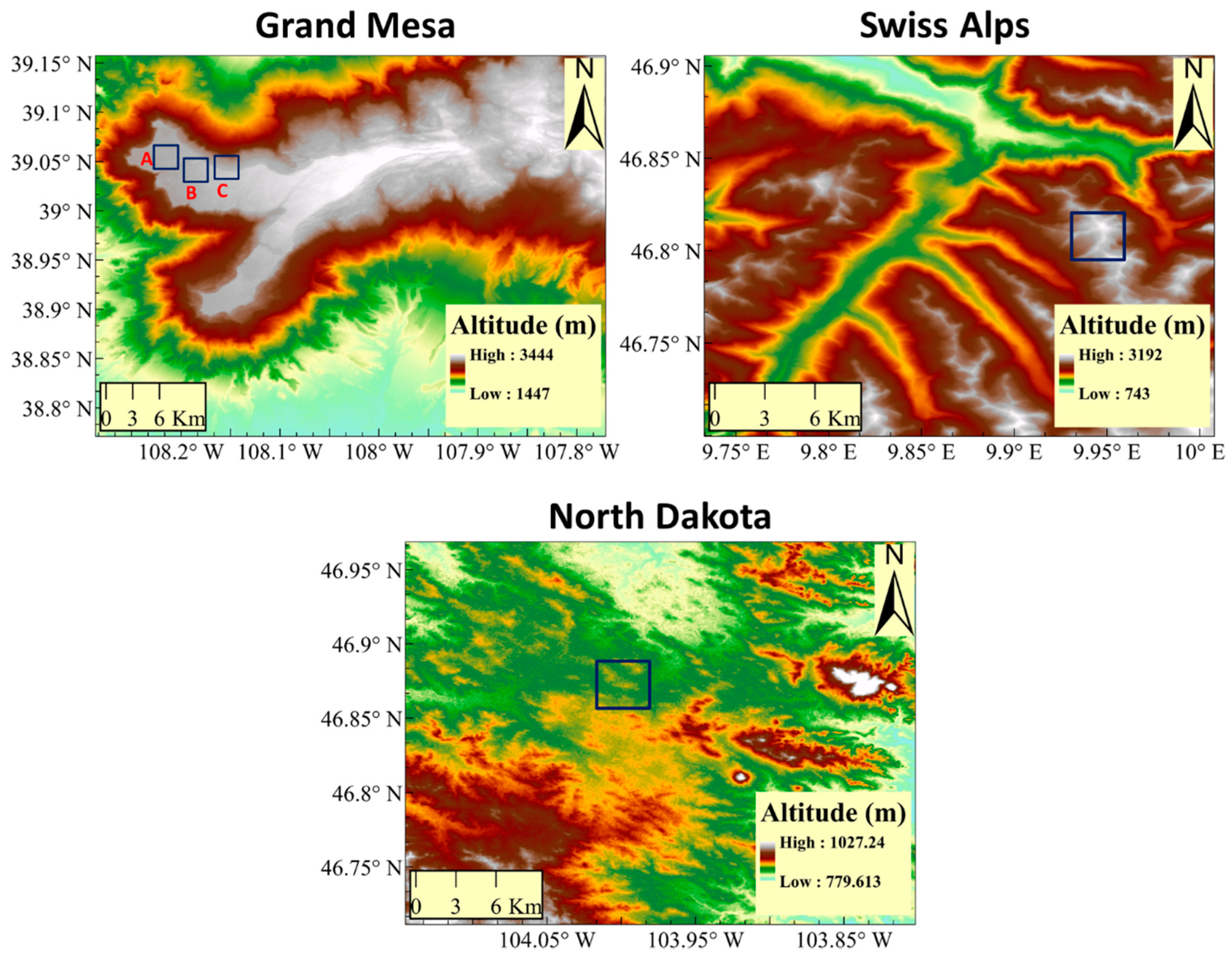
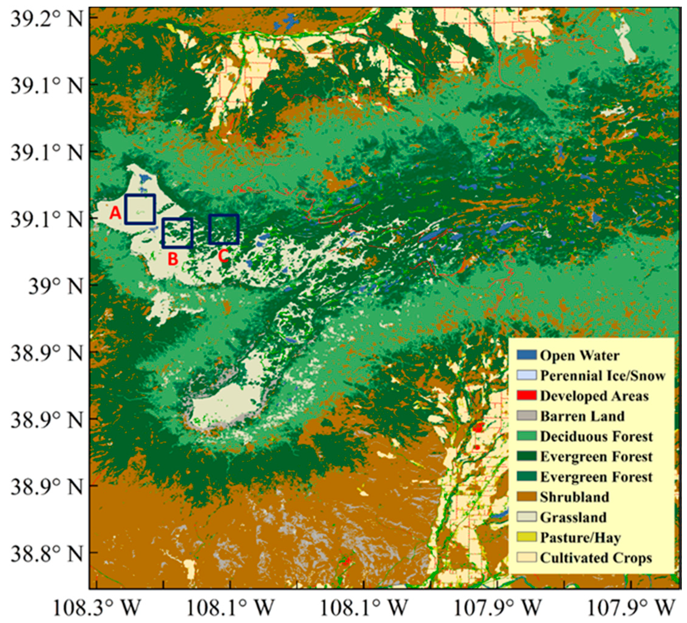
2.1. Study Regions
2.2. Data
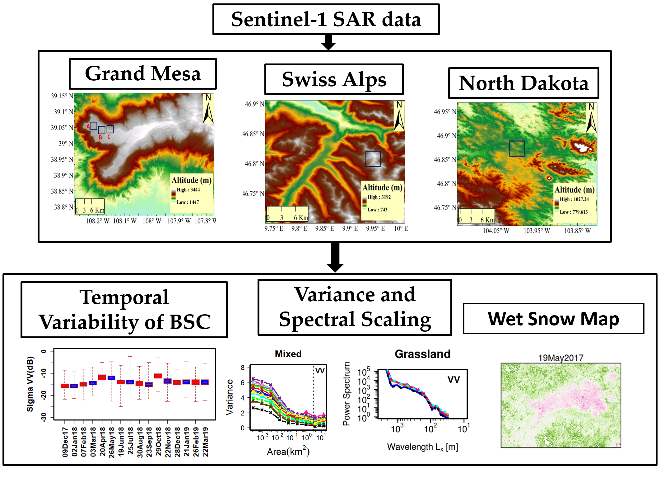
3. Methods
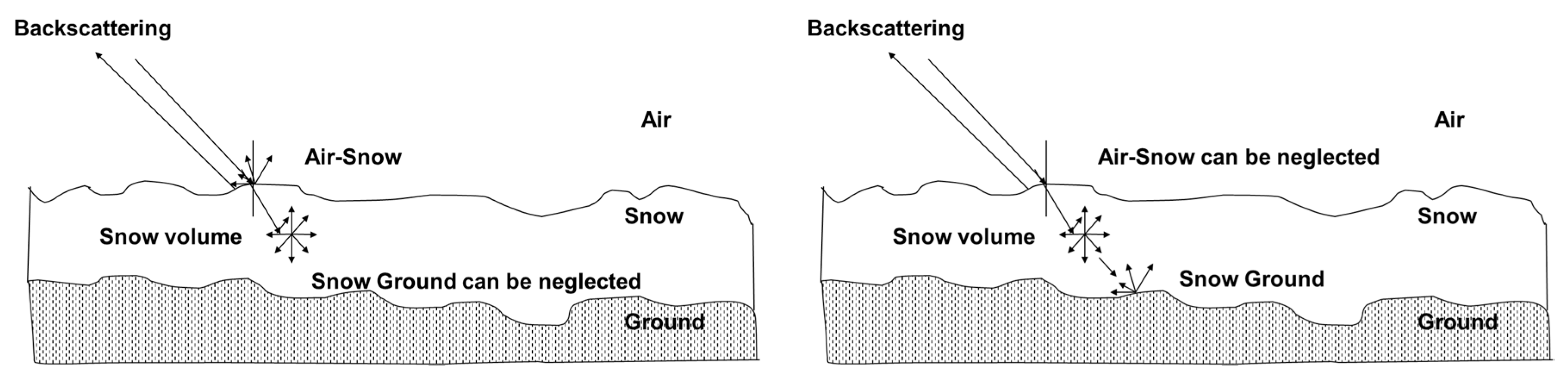
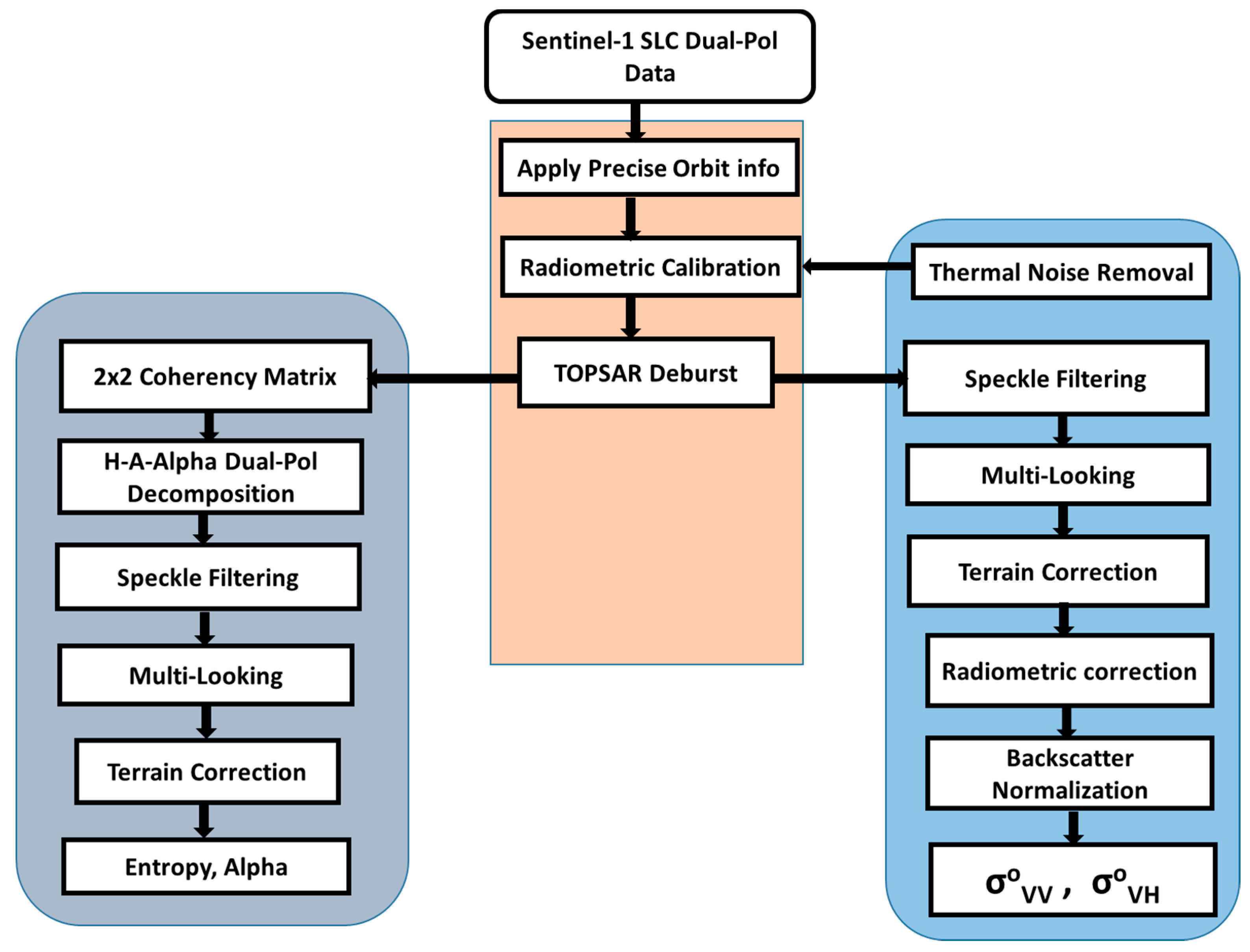
3.1. Backscattering Coefficient Estimation
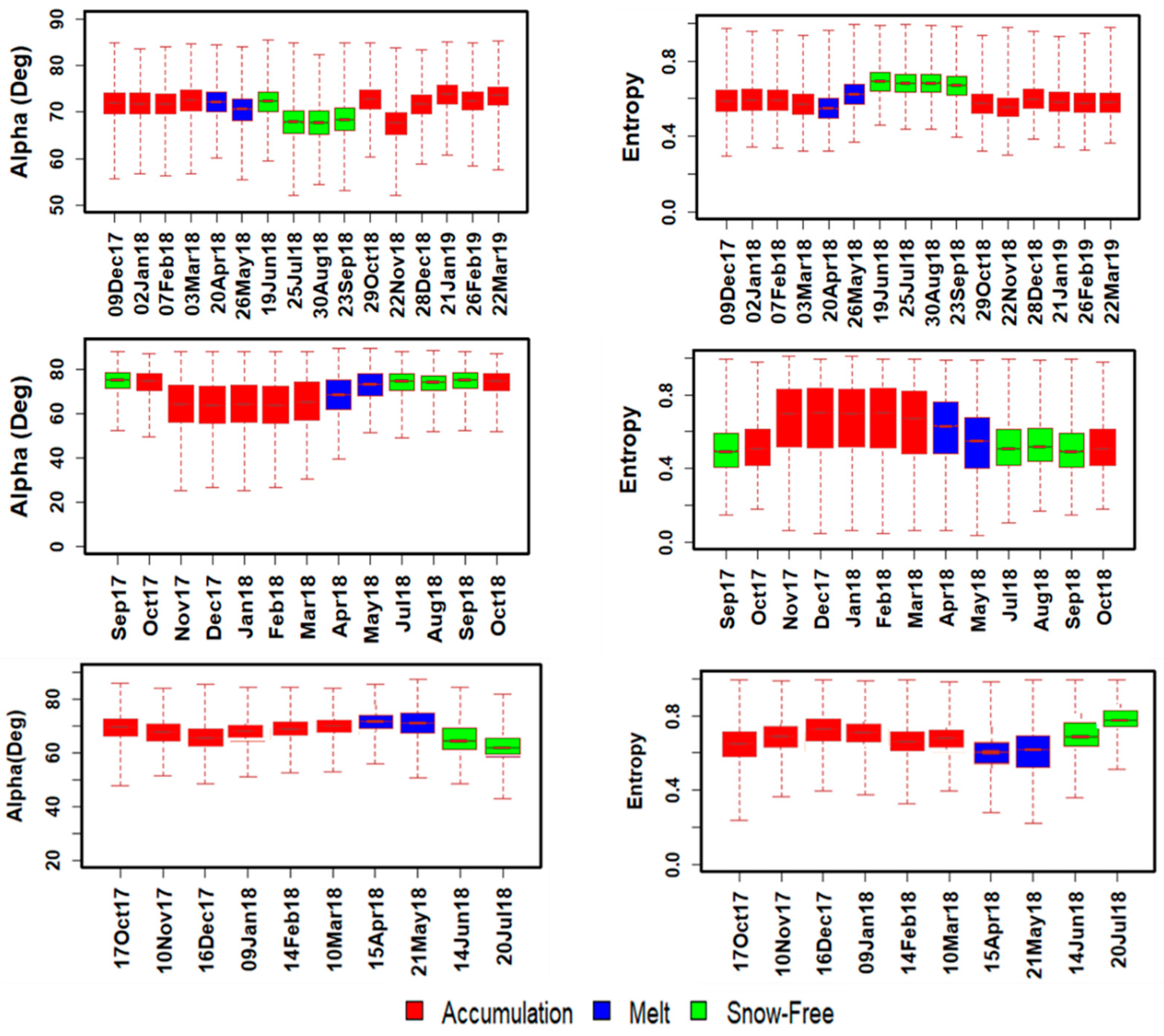
3.2. Coherency Metrics (Entropy–Alpha Estimation)
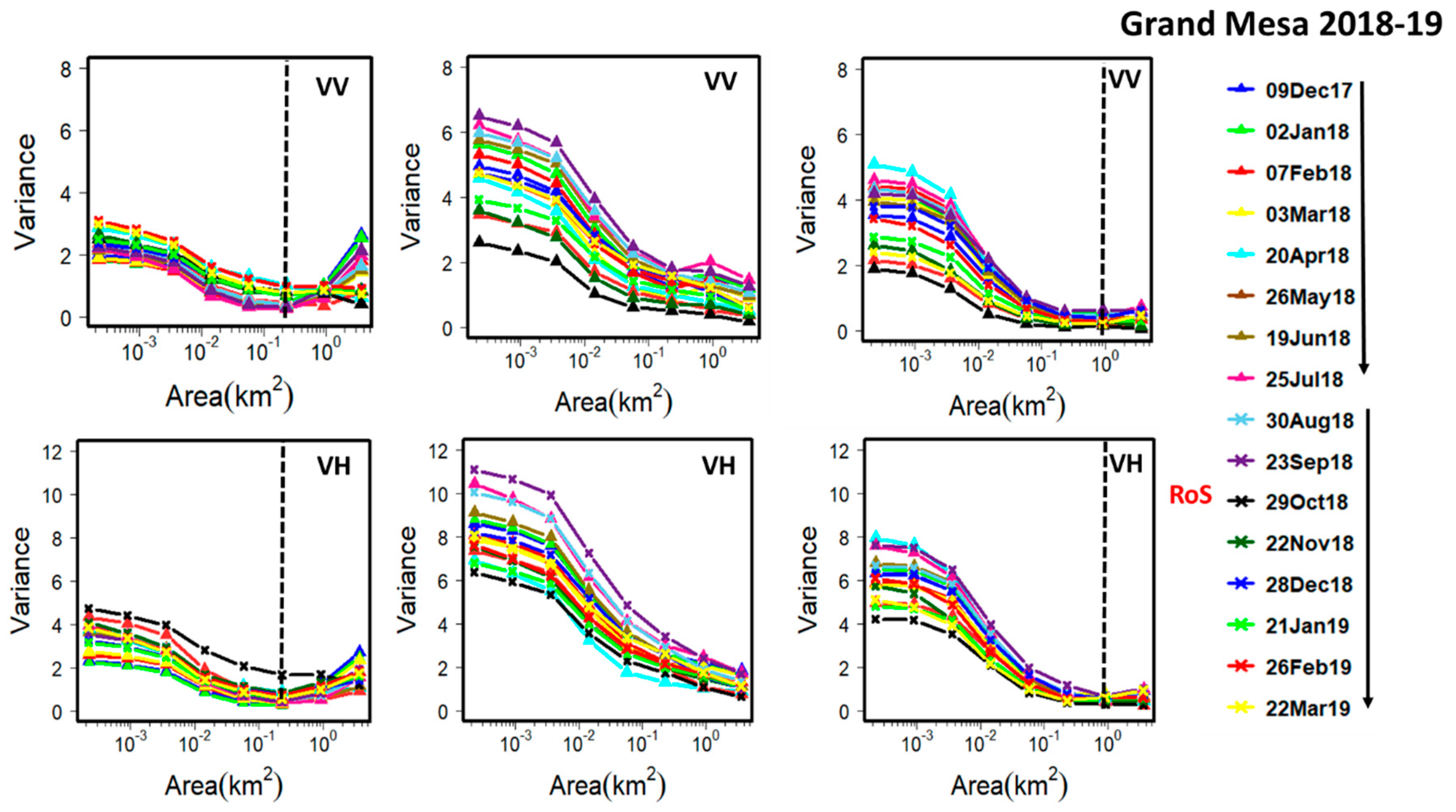
3.3. Scaling Analyses
3.4. Snow Wetness Mapping
4. Results and Discussion
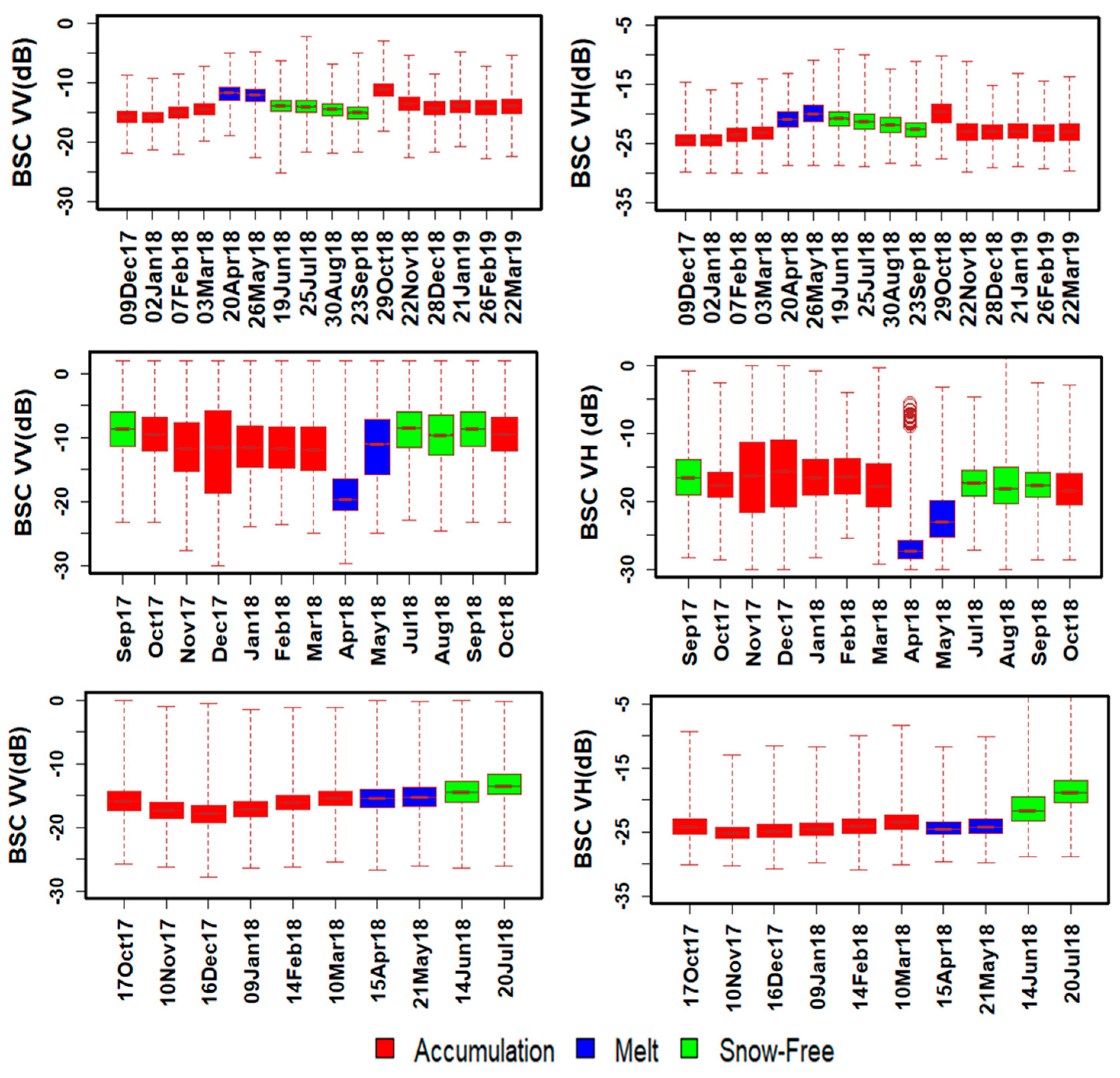
4.1. Temporal Variability of SAR Measurements over Complex Terrain
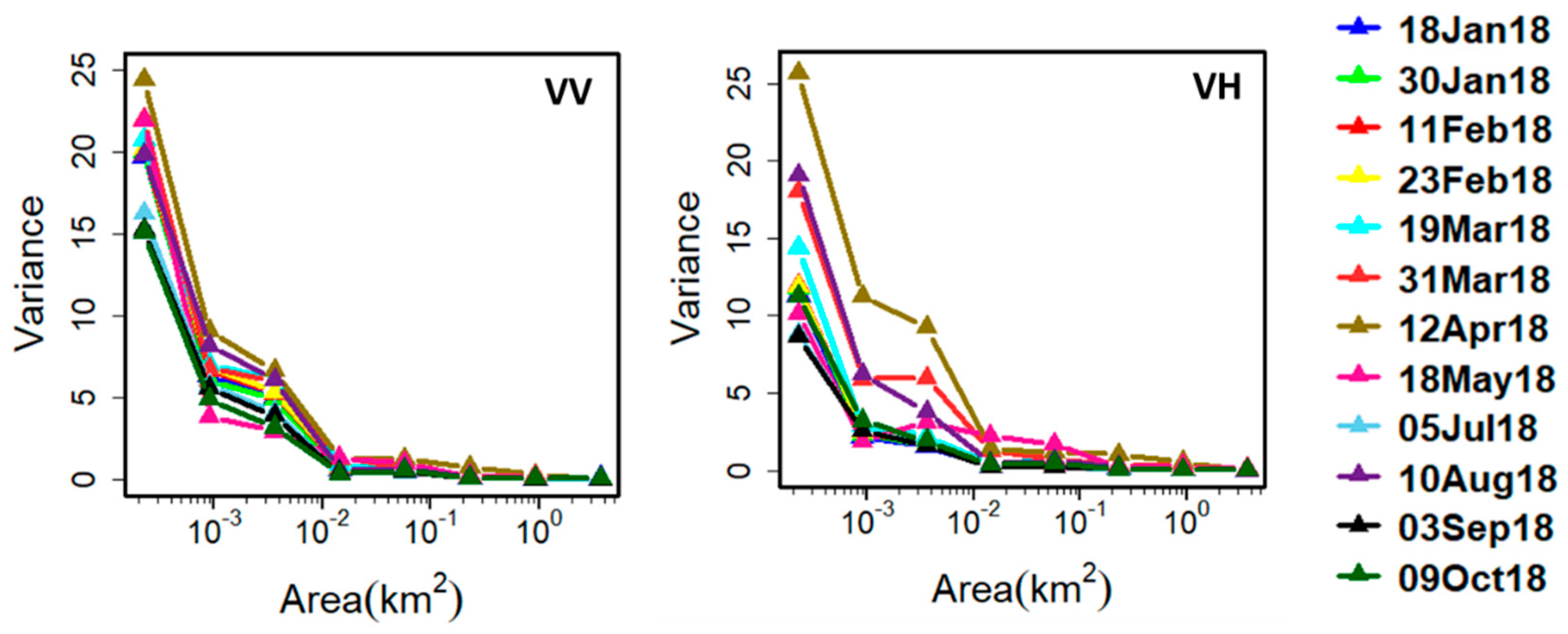
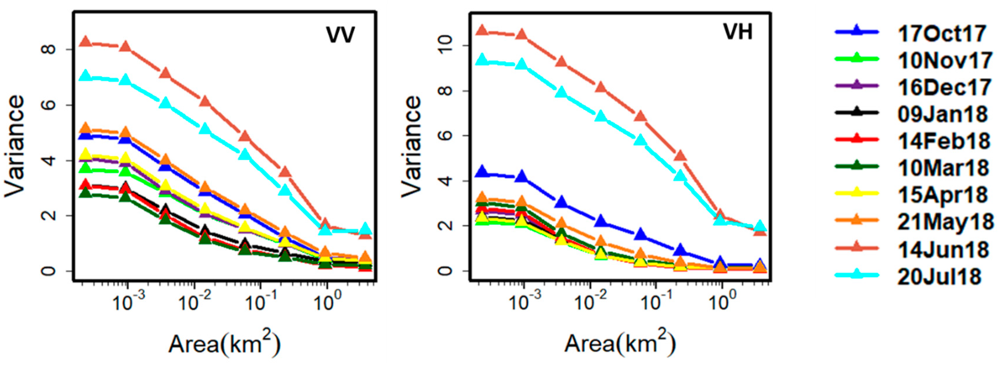
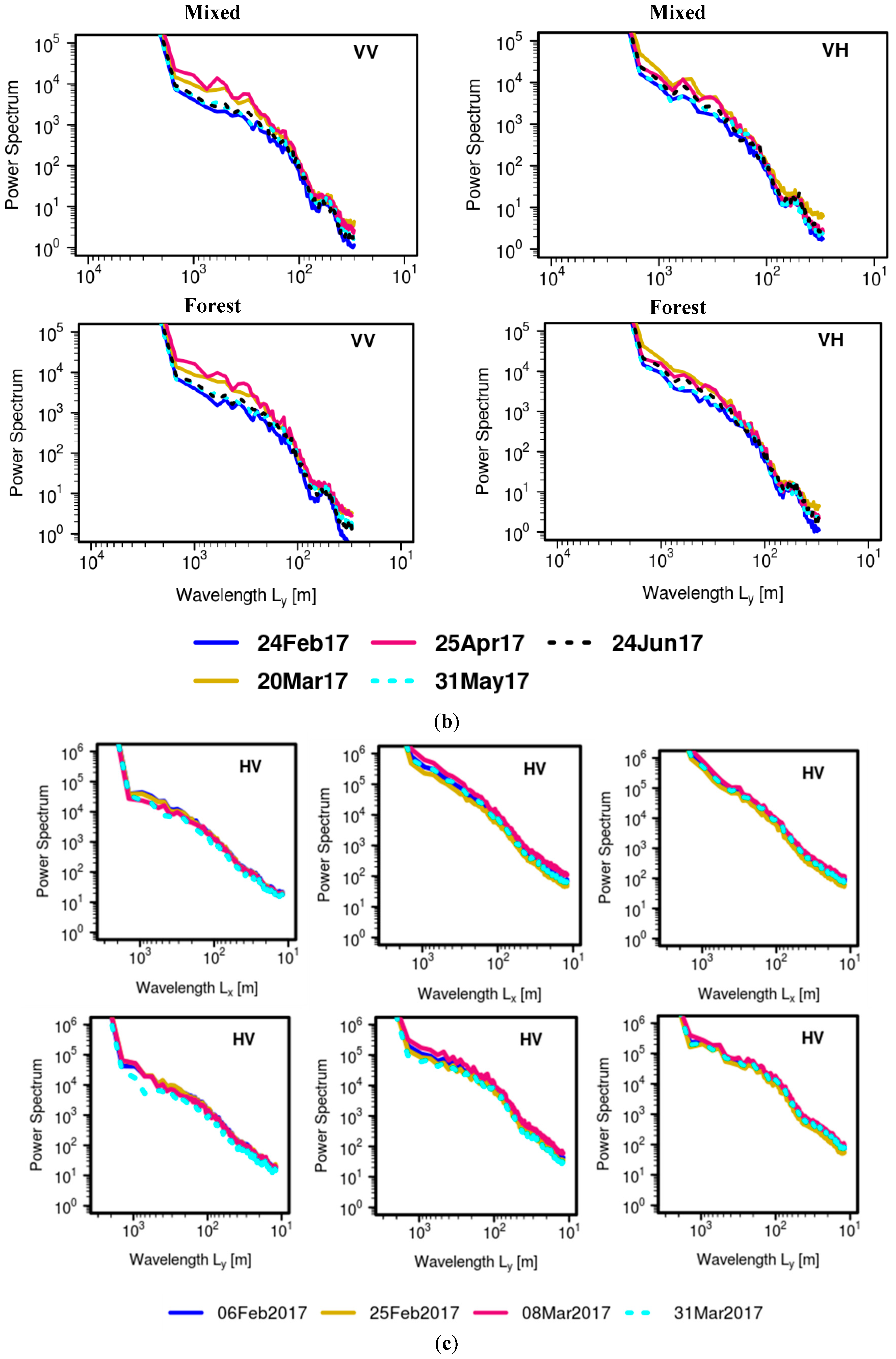
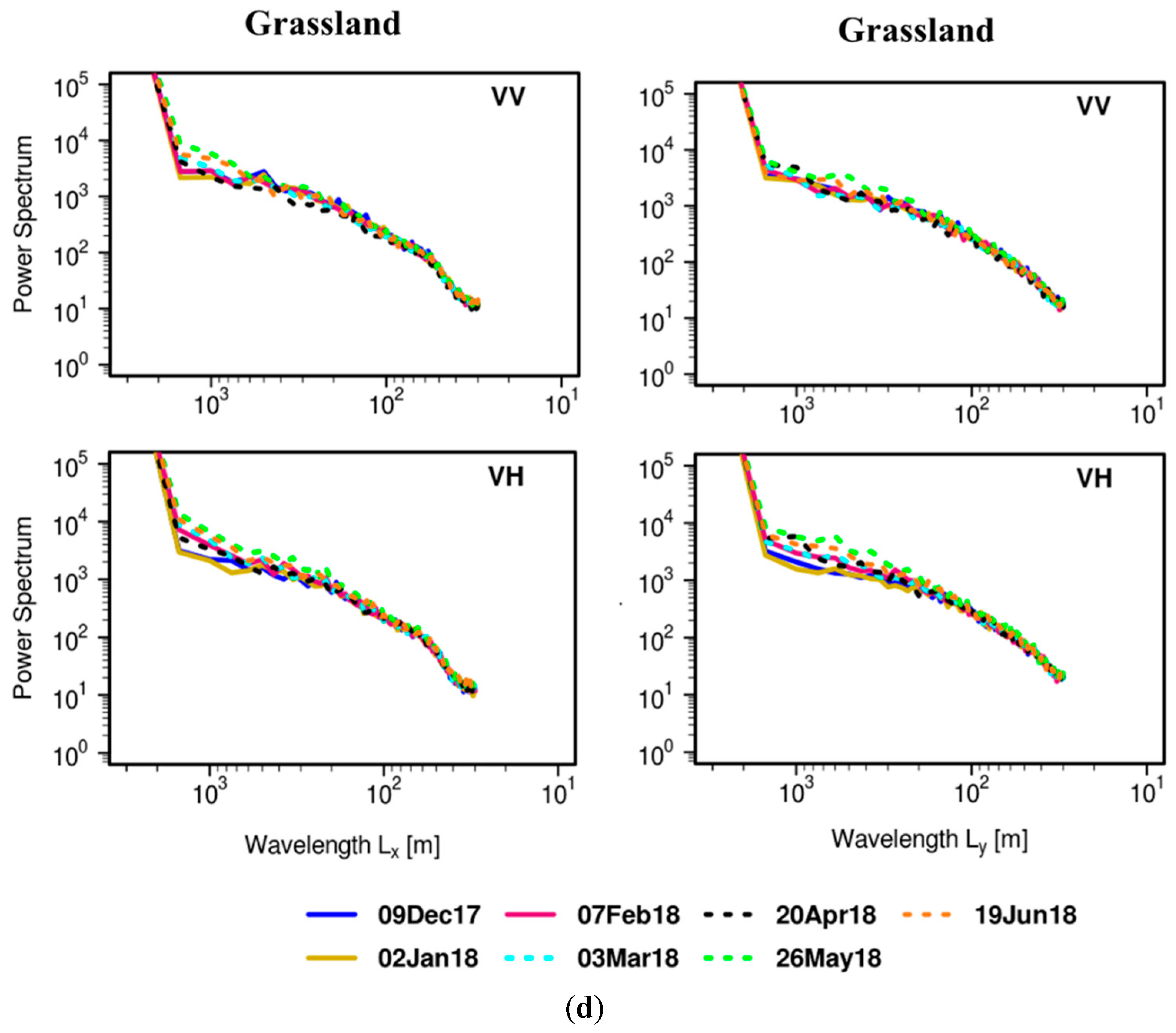
4.2. Space-Time Scaling Behavior
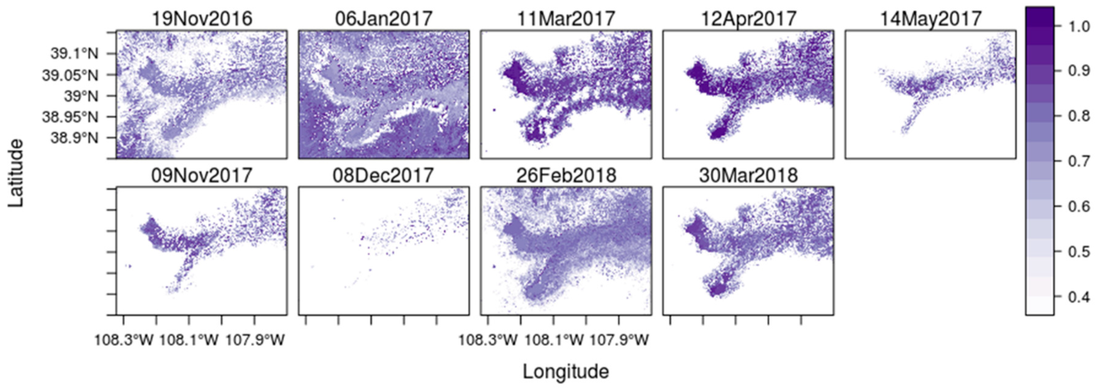
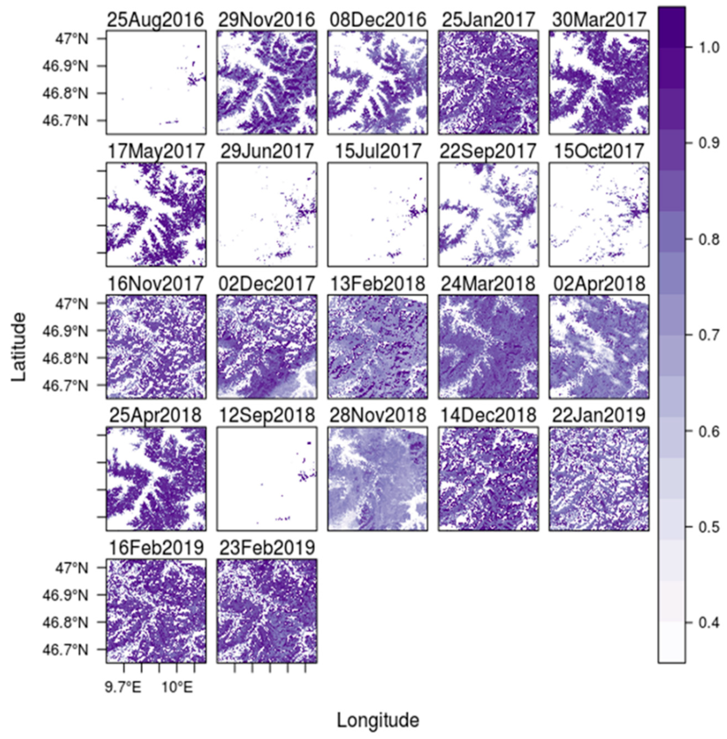
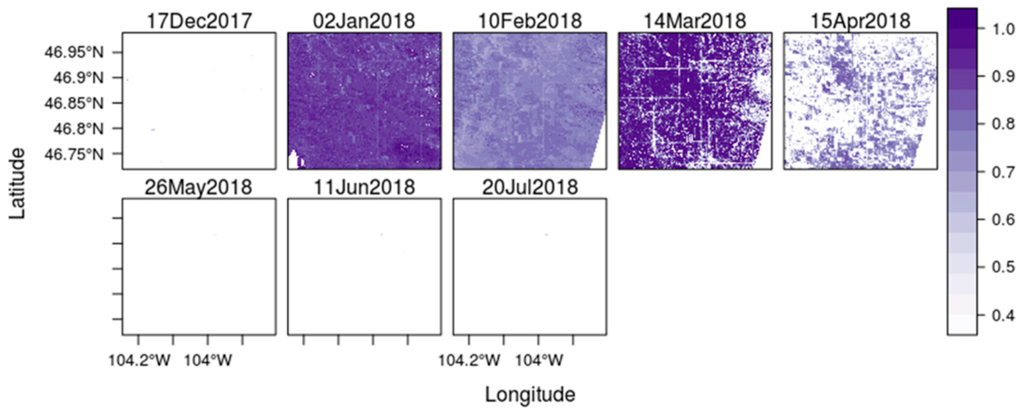
4.3. Wet Snow Mapping
5. Conclusions
Supplementary Materials
Author Contributions
Funding
Acknowledgments
Conflicts of Interest
References
- Brown, R.D.; Mote, P.W. The response of Northern Hemisphere snow cover to a changing climate. J. Clim. 2009, 22, 2124–2145. [Google Scholar] [CrossRef]
- Derksen, C.; Brown, R. Spring snow cover extent reductions in the 2008–2012 period exceeding climate model projections. Geophys. Res. Lett. 2012, 39. [Google Scholar] [CrossRef] [Green Version]
- Kevin, J.-P.W.; Kotlarski, S.; Scherrer, S.C.; Schär, C. The Alpine snow-albedo feedback in regional climate models. Clim. Dyn. 2017, 48, 1109–1124. [Google Scholar]
- Duffy, G.; Bennartz, R. The Role of Melting Snow in the Ocean Surface Heat Budget. Geophys. Res. Lett. 2018, 45, 9782–9789. [Google Scholar] [CrossRef]
- Ballesteros-Cánovas, J.; Trappmann, D.; Madrigal-González, J.; Eckert, N.; Stoffel, M. Climate warming enhances snow avalanche risk in the Western Himalayas. Proc. Natl. Acad. Sci. USA 2018, 115, 3410–3415. [Google Scholar] [CrossRef] [Green Version]
- Jeelani, G.; Feddema, J.J.; Veen, C.J.; Stearns, L. Role of snow and glacier melt in controlling river hydrology in Liddar watershed (western Himalaya) under current and future climate. Water Resour. Res. 2012, 48. [Google Scholar] [CrossRef] [Green Version]
- Jamieson, B. Formation of refrozen snowpack layers and their role in slab avalanche release. Rev. Geophys. 2006, 44. [Google Scholar] [CrossRef]
- Kang, D.-H.; Barros, A.P.; Kim, E.J. Evaluating Multispectral Snowpack Reflectivity With Changing Snow Correlation Lengths. IEEE Trans. Geosci. Remote Sens. 2016, 54, 7378–7384. [Google Scholar] [CrossRef]
- Wegmüller, U. The effect of freezing and thawing on the microwave signatures of bare soil. Remote Sens. Environ. 1990, 33, 123–135. [Google Scholar] [CrossRef]
- Matzler, C.; Strozzi, T.; Weise, T.; Floricioiu, D.-M.; Rott, H. Microwave snowpack studies made in the Austrian Alps during the SIR-C/X-SAR experiment. Int. J. Remote Sens. 1997, 18, 2505–2530. [Google Scholar] [CrossRef]
- Singh, G.; Yamaguchi, Y.; Park, S.-E. Utilization of four-component scattering power decomposition method for glaciated terrain classification. Geocarto Int. 2011, 26, 377–389. [Google Scholar] [CrossRef]
- Foster, J.L.; Sun, C.; Walker, J.P.; Kelly, R.; Chang, A.; Dong, J.; Powell, H. Quantifying the uncertainty in passive microwave snow water equivalent observations. Remote Sens. Environ. 2005, 94, 187–203. [Google Scholar] [CrossRef]
- Kunzi, K.F.; Patil, S.; Rott, H. Snow-Cover Parameters Retrieved from Nimbus-7 Scanning Multichannel Microwave Radiometer (SMMR) Data. IEEE Trans. Geosci. Remote Sens. 1982, GE-20, 452–467. [Google Scholar] [CrossRef]
- Pulliainen, J.; Hallikainen, M. Retrieval of regional snow water equivalent from space-borne passive microwave observations. Remote Sens. Environ. 2001, 75, 76–85. [Google Scholar] [CrossRef]
- Tait, A.B. Estimation of snow water equivalent using passive microwave radiation data. Remote Sens. Environ. 1998, 64, 286–291. [Google Scholar] [CrossRef]
- Tong, J.; Déry, S.J.; Jackson, P.L.; Derksen, C. Testing snow water equivalent retrieval algorithms for passive microwave remote sensing in an alpine watershed of western Canada. Can. J. Remote Sens. 2010, 36, S74–S86. [Google Scholar] [CrossRef]
- Ulaby, F.T.; Stiles, W.H. The active and passive microwave response to snow parameters: 2. Water equivalent of dry snow. J. Geophys. Res. Oceans 1980, 85, 1045–1049. [Google Scholar] [CrossRef]
- Bernier, P.Y. Microwave Remote Sensing of Snowpack Properties: Potential and Limitations. Hydrol. Res. 1987, 18, 1–20. [Google Scholar] [CrossRef]
- Niang, M.; Dedieu, J.-P.; Durand, Y.; Mérindol, L.; Bernier, M.; Dumont, M. New inversion method for snow density and snow liquid water content retrieval using C-band data from ENVISAT/ASAR alternating polarization in alpine environment. In Proceedings of the Proceedings of the 2007 ENVISAT Symposium, Montreux, Switzerland, 23–27 April 2007. [Google Scholar]
- Rott, H.; Domik, G.; Matzler, C.; Miller, H. Study on Use and Characteristics of SAR for Land Snow and Ice Applications; Institut fur Meteorologie und Geophysik, Universität Innsbruck: Innsbruck, Austria, 1985. [Google Scholar]
- Yan, B.; Weng, F.; Meng, H. Retrieval of snow surface microwave emissivity from the advanced microwave sounding unit. J. Geophys. Res. Atmos. 2008, 113. [Google Scholar] [CrossRef]
- Arslan, AN.; Hallikainen, M.T.; Pulliainen, J.T. Investigating of snow wetness parameter using a two-phase backscattering model. IEEE Trans Geosci Remote Sens 2005, 43, 1827–1833. [Google Scholar] [CrossRef]
- Baghdadi, N.; Gauthier, Y.; Bernier, M. Capability of multitemporal ERS-1 SAR data for wet-snow mapping. Remote Sens. Environ. 1997, 60, 174–186. [Google Scholar] [CrossRef]
- Besic, N.; Vasile, G.; Chanussot, J.; Stankovic, S.; Boldo, D.; d’Urso, G. Wet snow backscattering sensitivity on density change for SWE estimation. In Proceedings of the 2013 IEEE International Geoscience and Remote Sensing Symposium (IGARSS), Melbourne, Australia, 21–26 July 2013; pp. 1174–1177. [Google Scholar]
- Nagler, T.; Rott, H. Retrieval of wet snow by means of multitemporal SAR data. IEEE Trans. Geosci. Remote Sens. 2000, 38, 754–765. [Google Scholar] [CrossRef]
- Nagler, T.; Rott, H.; Ripper, E.; Bippus, G.; Hetzenecker, M. Advancements for Snowmelt Monitoring by Means of Sentinel-1 SAR. Remote Sens. 2016, 8, 348. [Google Scholar] [CrossRef] [Green Version]
- Ulaby, F.T.; Stiles, W.H.; Abdelrazik, M. Snowcover Influence on Backscattering from Terrain. IEEE Trans. Geosci. Remote Sens. 1984, GE-22, 126–133. [Google Scholar] [CrossRef]
- Shi, J.; Dozier, J. Inferring snow wetness using C-band data from SIR-C’s polarimetric synthetic aperture radar. IEEE Trans. Geosci. Remote Sens. 1995, 33, 905–914. [Google Scholar]
- Surendar, M.; Bhattacharya, A.; Singh, G.; Yamaguchi, Y.; Venkataraman, G. Development of a snow wetness inversion algorithm using polarimetric scattering power decomposition model. Int. J. Appl. Earth Obs. Geoinf. 2015, 42, 65–75. [Google Scholar] [CrossRef]
- Strozzi, T.; Wiesmann, A.; Mätzler, C. Active microwave signatures of snow covers at 5.3 and 35 GHz. Radio Sci. 1997, 32, 479–495. [Google Scholar] [CrossRef]
- Shi, J.; Dozier, J. Estimation of snow water equivalence using SIR-C/X-SAR. II. Inferring snow depth and particle size. IEEE Trans. Geosci. Remote Sens. 2000, 38, 2475–2488. [Google Scholar]
- Tsang, L.; Kong, J.A.; Ding, K.-H. Scattering of Electromagnetic Waves: Theories and Applications; John Wiley & Sons: New York, NY, USA, 2004. [Google Scholar]
- Tsang, L.; Pan, J.; Liang, D.; Li, Z.; Cline, D.W.; Tan, Y. Modeling active microwave remote sensing of snow using dense media radiative transfer (DMRT) theory with multiple-scattering effects. IEEE Trans. Geosci. Remote Sens. 2007, 45, 990–1004. [Google Scholar] [CrossRef]
- Fung, A.K. Microwave Scattering and Emission Models and Their Applications; Artech House: Boston, MA, USA, 1994; Available online: https://us.artechhouse.com/Microwave-Scattering-and-Emission-Models-and-Their-Applications-P748.aspx (accessed on 2 December 2019).
- Williams, L.D.; Gallagher, J.G.; Sugden, D.E.; Birnie, R.V. Surface snow properties effect on millimeter-wave backscatter. IEEE Trans. Geosci. Remote Sens. 1988, 26, 300–306. [Google Scholar] [CrossRef]
- Bernier, M.; Fortin, J.P. The potential of times series of C-Band SAR data to monitor dry and shallow snow cover. IEEE Trans. Geosci. Remote Sens. 1998, 36, 226–243. [Google Scholar] [CrossRef]
- Matzler, C. Microwave permittivity of dry snow. IEEE Trans. Geosci. Remote Sens. 1996, 34, 573–581. [Google Scholar] [CrossRef]
- Strozzi, T.; Matzler, C. Backscattering measurements of alpine snowcovers at 5.3 and 35 GHz. IEEE Trans. Geosci. Remote Sens. 1998, 36, 838–848. [Google Scholar] [CrossRef]
- He, G.; Feng, X.; Xiao, P.; Xia, Z.; Wang, Z.; Chen, H.; Li, H.; Guo, J. Dry and wet snow cover mapping in mountain areas using SAR and optical remote sensing data. IEEE J. Sel. Top. Appl. Earth Obs. Remote Sens. 2017, 10, 2575–2588. [Google Scholar] [CrossRef]
- National Academies of Sciences, Engineering, and Medicine. Thriving on Our Changing Planet: A Decadal Strategy for Earth Observation from Space; National Academies Press: Washington, DC, USA, 2019; ISBN 0-309-46757-8. [Google Scholar]
- Woodruff, C.D.; Qualls, R.J. Recurrent Snowmelt Pattern Synthesis Using Principal Component Analysis of Multiyear Remotely Sensed Snow Cover. Water Resour. Res. 2019, 55, 6869–6885. [Google Scholar] [CrossRef]
- Brucker, L.; Hiemstra, C.; Marshall, H.; Elder, K.; Roo, R.D.; Mousavi, M.; Bliven, F.; Peterson, W.; Deems, J.; Gadomski, P.; et al. Nasa Snowex’17 in SITU Measurements and Ground-Based Remote Sensing. In Proceedings of the IGARSS 2018 - 2018 IEEE International Geoscience and Remote Sensing Symposium, Valencia, Spain, 22–27 July 2018; pp. 6266–6268. [Google Scholar]
- Kim, E.; Gatebe, C.; Hall, D.; Newlin, J.; Misakonis, A.; Elder, K.; Marshall, H.P.; Hiemstra, C.; Brucker, L.; De Marco, E.; et al. NASA’s SnowEx campaign: Observing seasonal snow in a forested environment. In Proceedings of the 2017 IEEE International Geoscience and Remote Sensing Symposium (IGARSS), Fort Worth, TX, USA, 23–28 July 2017; pp. 1388–1390. [Google Scholar]
- Beniston, M.; Keller, F.; Goyette, S. Snow Pack in the Swiss Alps Under Changing Climatic Conditions: An Empirical Approach for Climate Impacts Studies. Theor. Appl. Climatol. 2003, 74, 19–31. [Google Scholar] [CrossRef]
- Coulter, L.L.; Stow, D.A.; Tsai, Y.-H.; Ibanez, N.; Shih, H.; Kerr, A.; Benza, M.; Weeks, J.R.; Mensah, F. Classification and assessment of land cover and land use change in southern Ghana using dense stacks of Landsat 7 ETM+ imagery. Remote Sens. Environ. 2016, 184, 396–409. [Google Scholar] [CrossRef]
- Zan, F.D.; Guarnieri, A.M. TOPSAR: Terrain Observation by Progressive Scans. IEEE Trans. Geosci. Remote Sens. 2006, 44, 2352–2360. [Google Scholar] [CrossRef]
- Lee, J.; Ainsworth, T.L.; Wang, Y.; Chen, K. Polarimetric SAR Speckle Filtering and the Extended Sigma Filter. IEEE Trans. Geosci. Remote Sens. 2015, 53, 1150–1160. [Google Scholar] [CrossRef]
- Kellndorfer, J.M.; Pierce, L.E.; Dobson, M.C.; Ulaby, F.T. Toward consistent regional-to-global-scale vegetation characterization using orbital SAR systems. IEEE Trans. Geosci. Remote Sens. 1998, 36, 1396–1411. [Google Scholar] [CrossRef]
- Ulaby, F.T.M. Microwave Remote Sensing: Active and Passive. Volume 1 - Microwave Remote Sensing Fundamentals and Radiometry; Addison-Wesley: Reading, MA, USA, 1981. [Google Scholar]
- Cloude, S.R.; Pottier, E. An entropy based classification scheme for land applications of polarimetric SAR. IEEE Trans. Geosci. Remote Sens. 1997, 35, 68–78. [Google Scholar] [CrossRef]
- Cloude, S.R.; Pottier, E. A review of target decomposition theorems in radar polarimetry. IEEE Trans. Geosci. Remote Sens. 1996, 34, 498–518. [Google Scholar] [CrossRef]
- Muhuri, A.; Manickam, S.; Bhattacharya, A. Scattering Mechanism Based Snow Cover Mapping Using RADARSAT-2 C-Band Polarimetric SAR Data. IEEE J. Sel. Top. Appl. Earth Obs. Remote Sens. 2017, 10, 3213–3224. [Google Scholar] [CrossRef]
- Park, S.; Yamaguchi, Y.; Singh, G.; Yamaguchi, S.; Whitaker, A.C. Polarimetric SAR Response of Snow-Covered Area Observed by Multi-Temporal ALOS PALSAR Fully Polarimetric Mode. IEEE Trans. Geosci. Remote Sens. 2014, 52, 329–340. [Google Scholar] [CrossRef]
- Singh, G.; Venkataraman, G.; Yamaguchi, Y.; Park, S. Capability Assessment of Fully Polarimetric ALOS–PALSAR Data for Discriminating Wet Snow from Other Scattering Types in Mountainous Regions. IEEE Trans. Geosci. Remote Sens. 2014, 52, 1177–1196. [Google Scholar] [CrossRef]
- Kim, G.; Barros, A.P. Space–time characterization of soil moisture from passive microwave remotely sensed imagery and ancillary data. Remote Sens. Environ. 2002, 81, 393–403. [Google Scholar] [CrossRef]
- Eghdami, M.; Barros, A.P. Extreme Orographic Rainfall in the Eastern Andes Tied to Cold Air Intrusions. Front. Environ. Sci. Lausanne 2019. [Google Scholar] [CrossRef]
- Nogueira, M.; Barros, A.P.; Miranda, P. Multifractal properties of embedded convective. structures in orographic precipitation: Toward subgrid-scale predictability. Nonlinear Process. Geophys. 2013, 20, 1–17. [Google Scholar] [CrossRef]
- Quegan, S.; Yu, J.J. Filtering of multichannel SAR images. IEEE Trans. Geosci. Remote Sens. 2001, 39, 2373–2379. [Google Scholar] [CrossRef]
- Rott, H. The analysis of backscattering properties from SAR data of mountain regions. IEEE J. Ocean. Eng. 1984, 9, 347–355. [Google Scholar] [CrossRef]
- Lievens, H.; Demuzere, M.; Marshall, H.-P.; Reichle, R.H.; Brucker, L.; Brangers, I.; de Rosnay, P.; Dumont, M.; Girotto, M.; Immerzeel, W.W.; et al. Snow depth variability in the Northern Hemisphere mountains observed from space. Nat. Commun. 2019, 10. [Google Scholar] [CrossRef] [PubMed]
- Rignot, E.; Way, J.B. Monitoring freeze-thaw cycles along North-South Alaskan transects using ERS-1 SAR. Remote Sens. Environ. 1994, 49, 131–137. [Google Scholar] [CrossRef] [Green Version]
- Evans, S. Dielectric Properties of Ice and Snow–a Review. J. Glaciol. 1965, 5, 773–792. [Google Scholar] [CrossRef] [Green Version]
- Kang, D.H.; Barros, A.P.; Dery, S.J. Evaluating passive microwave radiometry for the dynamical transition from dry to wet snowpacks. IEEE Trans. Geosci. Remote Sens. 2013, 52, 3–15. [Google Scholar] [CrossRef]
- Mätzler, C. Applications of the interaction of microwaves with the natural snow cover. Remote Sens. Rev. 1987, 2, 259–387. [Google Scholar] [CrossRef]
- Zahnen, N.; Jung-Rothenhäusler, F.; Oerter, H.; Wilhelms, F.; Miller, H. Correlation between Antarctic dry snow properties and backscattering characteristics in RADARSAT SAR imagery. In Proceedings of the Proceedings of EARSeL-LISSIG-Workshop Observing our Cryosphere from Space, Bern, Switzerland, 11–13 March 2002; Volume 141. [Google Scholar]
- Sturm, M.; Wagner, A.M. Using repeated patterns in snow distribution modeling: An Arctic example. Water Resour. Res. 2010, 46. [Google Scholar] [CrossRef] [Green Version]
- Kuligowski, R.J.; Barros, A.P. Blending multiresolution satellite data with application to the initialization of an orographic precipitation model. J. Appl. Meteorol. 2001, 40, 1592–1606. [Google Scholar] [CrossRef]
- Bindlish, R.; Barros, A.P. Subpixel variability of remotely sensed soil moisture: An inter-comparison study of SAR and ESTAR. IEEE Trans. Geosci. Remote Sens. 2002, 40, 326–337. [Google Scholar] [CrossRef]
- Tao, K.; Barros, A.P. Using fractal downscaling of satellite precipitation products for hydrometeorological applications. J. Atmos. Ocean. Technol. 2010, 27, 409–427. [Google Scholar] [CrossRef] [Green Version]
- Anderson, B.T.; McNamara, J.P.; Marshall, H.-P.; Flores, A.N. Insights into the physical processes controlling correlations between snow distribution and terrain properties. Water Resour. Res. 2014, 50, 4545–4563. [Google Scholar] [CrossRef]
- Marin, C.; Bertoldi, G.; Premier, V.; Callegari, M.; Brida, C.; Hürkamp, K.; Tschiersch, J.; Zebisch, M.; Notarnicola, C. Use of Sentinel-1 radar observations to evaluate snowmelt dynamics in alpine regions. Available online: https://pdfs.semanticscholar.org/f6f1/16334e5f0f4664ce8b50dadf348527a0b553.pdf (accessed on 2 December 2019).


| Year | Mode | Polarization | Incidence Angle Range | Acquisition Dates |
|---|---|---|---|---|
| 2017 | Interferometric Swath | VV, VH | 38.7–46.3 | 07 Jan, 24 Feb, 08 Mar, 20 Mar, 01 Apr, 25 Apr, 07 May, 31 May, 24 Jun |
| 2018 | Interferometric Swath | VV, VH | 38.7–46.3 | 02 Jan, 07 Feb, 03 Mar, 20 Apr, 26 May, 19 Jun, 25 Jul, 30 Aug, 23 Sep, 29 Oct, 22 Nov, 28 Dec |
| 2019 | Interferometric Swath | VV, VH | 38.7–46.3 | 21 Jan, 26 Feb, 22 Mar |
| Year | Mode | Polarization | Incidence Angle Range | Acquisition Dates |
|---|---|---|---|---|
| 2018 | Interferometric Swath | VV, VH | 30.4–46.0 | 18 Jan, 30 Jan, 11 Feb, 23 Feb, 19 Mar, 31 Mar, 12 Apr, 06 May, 18 May, 30 May, 10 Aug |
| Year | Mode | Polarization | Incidence Angle Range | Acquisition Dates |
|---|---|---|---|---|
| 2017 | Interferometric Swath | VV, VH | 30.4–46.0 | 17 Oct, 10 Nov, 16 Dec |
| 2018 | Interferometric Swath | VV, VH | 30.4–46.0 | 19 Jan, 14 Feb, 10 Mar, 15 Apr, 21 May, 14 Jun, 20 Jul |
| Region | Year | Acquisition Date |
|---|---|---|
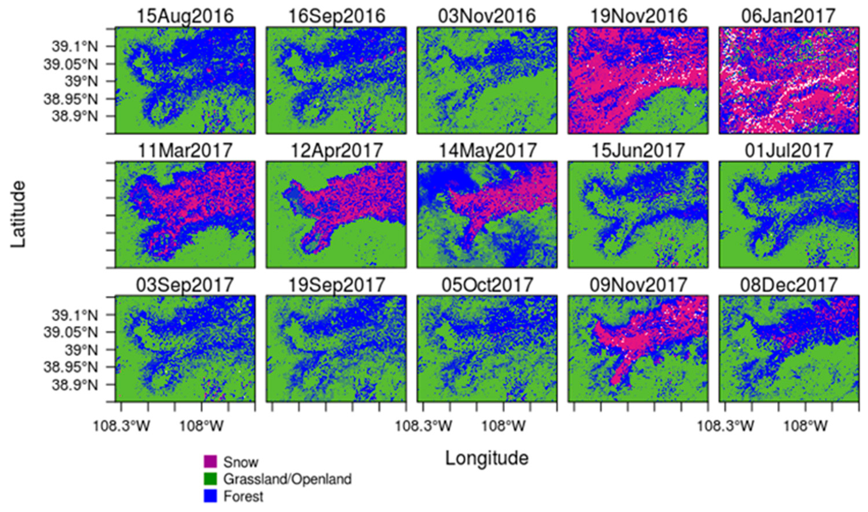
| Grand Mesa | 2016 | 15 Aug, 16 Sep, 03 Nov, 19 Nov |
| 2017 | 06 Jan, 11 Mar, 12 Apr, 14 May, 15 Jun, 01 Jul, 03 Sep, 05 Oct, 09 Nov, 08 Dec | |
| 2018 | 26 Feb, 30 Mar, 17 May, 02 Jun, 04 Jul, 22 Sep, 25 Nov | |
| Swiss Alps | 2016 | 25 Aug, 29 Nov, 08 Dec |
| 2017 | 25 Jan, 30 Mar, 17 May, 29 Jun, 15 Jul, 22 Sep, 15 Oct, 16 Nov, 02 Dec | |
| 2018 | 13 Feb, 24 Mar, 02 Apr, 25 Apr, 12 Sep, 28 Nov, 14 Dec | |
| 2019 | 22 Jan, 16 Feb, 23 Feb | |
| North Dakota | 2017–2018 | 17 Dec, 02 Jan, 10 Feb, 14 Mar, 15 Apr, 26 May, 11 Jun, 20 Jul |
| Number of Pixels (Range Direction) | Number of Pixels (Azimuth Direction) | Total Number of Pixels | Pixel Area Range × Azimuth (m2) |
|---|---|---|---|
| 1 | 1 | 1 | 15 × 15 |
| 2 | 2 | 4 | 30 × 30 |
| 4 | 4 | 16 | 60 × 60 |
| 8 | 8 | 64 | 120 × 120 |
| 16 | 16 | 256 | 240 × 240 |
| 32 | 32 | 1024 | 480 × 480 |
| 64 | 64 | 4096 | 960 × 960 |
| 128 | 128 | 16,384 | 1920 × 1920 |
© 2020 by the authors. Licensee MDPI, Basel, Switzerland. This article is an open access article distributed under the terms and conditions of the Creative Commons Attribution (CC BY) license (http://creativecommons.org/licenses/by/4.0/).
Share and Cite
Manickam, S.; Barros, A. Parsing Synthetic Aperture Radar Measurements of Snow in Complex Terrain: Scaling Behaviour and Sensitivity to Snow Wetness and Landcover. Remote Sens. 2020, 12, 483. https://doi.org/10.3390/rs12030483
Manickam S, Barros A. Parsing Synthetic Aperture Radar Measurements of Snow in Complex Terrain: Scaling Behaviour and Sensitivity to Snow Wetness and Landcover. Remote Sensing. 2020; 12(3):483. https://doi.org/10.3390/rs12030483
Chicago/Turabian StyleManickam, Surendar, and Ana Barros. 2020. "Parsing Synthetic Aperture Radar Measurements of Snow in Complex Terrain: Scaling Behaviour and Sensitivity to Snow Wetness and Landcover" Remote Sensing 12, no. 3: 483. https://doi.org/10.3390/rs12030483
APA StyleManickam, S., & Barros, A. (2020). Parsing Synthetic Aperture Radar Measurements of Snow in Complex Terrain: Scaling Behaviour and Sensitivity to Snow Wetness and Landcover. Remote Sensing, 12(3), 483. https://doi.org/10.3390/rs12030483