Monitoring Three-Decade Expansion of China’s Major Cities Based on Satellite Remote Sensing Images

1
School of Resource and Environmental Sciences, Wuhan University, Wuhan 430079, China
2
State Key Laboratory of Information Engineering in Surveying, Mapping and Remote Sensing, Wuhan University, Wuhan 430079, China
3
The Collaborative Innovation Center for Geospatial Technology, Wuhan 430079, China
4
School of Urban Design, Wuhan University, Wuhan 430072, China
5
Changjiang River Scientific Research Institute, Changjiang Water Resources Commission, Wuhan 430015, China
*
Author to whom correspondence should be addressed.
Remote Sens. 2020, 12(3), 491; https://doi.org/10.3390/rs12030491
Submission received: 15 December 2019
/
Revised: 25 January 2020
/
Accepted: 2 February 2020
/
Published: 4 February 2020
(This article belongs to the Section Urban Remote Sensing)
Abstract
:As the largest developing country, China has experienced dramatic urban expansion since the “reform and opening-up” policy started at the end of the 1970s. In this paper, we monitor three decades of urban expansion in China’s 36 major cities, based on the spectral mixture analysis of remotely sensed satellite images. The results demonstrated that these major cities have expanded by 5.85 times from 1986 to 2015, with 15.51 km2 average expansion area per city per year. We found the urban expansion trajectories showed three different modes, i.e., exponential, linear and s-shaped, which were closely related to the city development level. In the old city zones, however, there was an interesting common tendency of the impervious surface area (ISA) first increasing and then decreasing, which could be largely attributed to the phenomenon of urban village reconstruction in China’s cities. Based on the Granger Causality Test (GCT), the interaction between urban ISA and Gross Domestic Product (GDP) per capita (GDPPC) suggested that the former was the driver of the latter. Meanwhile, taking the Yangtze River as the division between north and south China, there exists a north–south territorial differentiation for the interaction between ISA and total population at the year-end (TP).

1. Introduction
Urbanization can be expressed as a shift of population from rural to urban areas, predominantly resulting in a transformation from rural land to urban land [1,2,3,4]. According to the United Nations, by 2014, 54% of the world population had lived in an urban area [5], and this is predicted to reach 66% by 2050. The growth of the urban population inevitably results in urban area expansion. It has been reported that the global urban area is likely to increase by 1.2 million km2 by 2030 [6]. Although urban areas represent a small fraction of the Earth’s surface, they have global impacts, including natural land loss, food waste, ecological degradation, environmental pollution, and so on [4,6,7,8,9,10].
Remotely sensed data, with superiority of short update cycle, continuous functioning and large coverage [11], has become an important means for urban studies around the world, especially for large-scale monitoring. At a global scale, the global urban areas have been measured at coarse spatial resolution by optical remotesensing data [12,13,14] or nighttime light data [15,16,17]. In recent years, to describe a more precise urban land, some researchers have measured the global urban extent at a 30 m resolution by Landsat data [18,19,20], the description for spatial distribution of urban area can therefore be further improved. At a continental scale, the urban areas of America [21,22,23], Asia [24,25,26], Europe [27,28,29], and Africa [30,31] have also been carefully discussed by satellite data. Those large-scale research studies have provided a macroscopic description of urban extent, inspiring us to explore the dynamics of urban expansion and the interaction between urban area and the environment. A more specific and typical area is therefore in need for more refined research.
Since the “reform and opening-up” policy started at the end of the 1970s, China has experienced unprecedented rapid urbanization [32,33,34,35]. It has been reported that China is responsible for much of the global urban expansion that has taken place over the past three decades [6,12,13,36]. Additionally, China will still play an important role in future global urban expansion. Thus, to deeply understand and deal with urbanization, it is of great importance to monitor and analyze the urban expansion progress in China.
Previous studies have discussed a lot on the dynamics and the related factors of urbanization. For the dynamics of urban expansion, spatial changes have attracted wide attention [15,37,38,39]. On the one hand, the relative position relation between the new urban patches and the former urban area has been discussed (e.g., infilling, edge-expansion, and leapfrogging) [5,40,41,42]. On the other hand, the different land changes (e.g., how many natural lands have been converted into built-up lands) for different cities or regions have been interpreted and compared by the Land Use and Land Cover (LULC) data [43,44,45,46]. For the interaction between urban area and the environment, many related factors for urbanization have been explored, such as, population, economy, industry, haze, and temperature etc. [47,48,49,50,51,52,53,54]. For example, Maitiniyazi Maimaitijiang et al. discussed the correlation between land cover categories and population changes [52]; Ahmed Mustafa et al. explored the relationship between different densities of urban development and many other socio-economic factors [53,54]. However, most of the interactions are expressed by correlation or regression analysis [55,56,57], which have focused on the correlation between the factors and urban expansion but neglected the causality.
By far, although the spatial distribution pattern is relatively well-acknowledged, we still have a limited understanding of the urban expansion trajectories [58] and its driving mechanisms [59]. Therefore, the main objective of this paper was to provide long-term (1986–2015) monitoring for China’s urbanization, especially concentrated on the urbanization patterns in time series. Utilizing Landsat remote sensing data covering 36 major cities in China from 1986 to 2015 (Table S1), we assessed the temporal urban expansion in China and three urban expansion trajectories were found. In particular, the early city core, i.e., the old city zone, may be a priceless record of urban development since it has been consistently regarded as the urban area along the urbanization progress, which deserves refined research. Thus, the temporal trends for impervious surface area (ISA) within the old city zones are discussed and a remarkable trend was found. Hence, we understand the temporal urbanization progress for the whole city and for the old city zone in China. Furthermore, to interpret the driving mechanisms for urbanization, we explored the potential cause and effect between the factors (population and economy) and urban ISA changes with the assistance of the Granger Causality Test (GCT).
2. Materials and Methods
Using Landsat remote sensing data (Landsat-5, Landsat-7, and Landsat-8) covering the 36 major cities in China from 1986 to 2015, we utilized linear spectral mixture analysis (LSMA) to extract the ISA for each city. The ISA was then used to generate the urban extent. With the assistance of statistical data, including GDP per capita and total population, GCT was conducted to investigate possible driving mechanisms for urban development.
2.1. Study Region and Data
The study region involved 36 major cities in mainland China (Figure 1). Given that China’s cities are administrative entities and officially designated according to political status, economic development level, and total population [60], these cities are capitals for 23 provinces, capitals for 5 autonomous regions, 4 municipalities, and 4 other sub-provincial cities. The study period was from 1986 to 2015, with a total length of 30 years.
The data used included two main parts. (1) Satellite data. Cloud-free Landsat images (digital number data) covering the 36 major cities in mainland China were obtained from the United States Geological Survey (USGS) website (http://glovis.usgs.gov/). One image was selected for one year. From Table S1, it could be found that more than 17 images were collected for the past three decades for each city, with a time span between two adjacent study years less than three years. (2) Statistical data. The statistical data (GDP and total population at the year-end) were obtained from the China City Statistical Yearbook (1987–2016). The result of GDP divided by total population was regarded as GDP per capita.
2.2. Data Preprocessing
Radiometric calibration, geometric rectification, mosaicking and clipping of images were all conducted. In detail, for each city, if the images were not georeferenced with each other, the image in the first study year was used as the reference to perform image-to-image registration, and then every image was clipped by the administrative district boundary. Image mosaicking was applied in Changchun and Shanghai. Moreover, to reduce the influence of atmospheric effects, the Fast Line-of-sight Atmospheric Analysis of Spectral Hypercubes (FLAASH) atmospheric correction algorithm was applied to all experimental images.
To acquire more experimental data, an image recovery [61,62] method was applied in this research. For the study period of 2003–2015, if the classification results for the available cloud-free Landsat images were not acceptable, and the time span between two adjacent study years was greater than three years, we filled the gaps in the SLC-off images following the image recovery method in [63,64] (software could be downloaded from http://sendimage.whu.edu.cn/en/resources/). The recovery method was applied in Hefei and Jinan. An example can be seen in Figure 2.
According to previous research, water bodies may be easily confused with the low-reflectance impervious surface [65]. The Normalized difference water index (NDWI) [66] was therefore used to exclude water bodies before conducting the urban area extraction. For each image, the NDWI threshold was set as 0,0.1,0.2,0.3,0.4, and 0.5, respectively. The best result with the least water bodies and the most impervious surface would be selected visually.
2.3. Urban Area Extraction
Various definitions for urban area will result in diverse estimates [41]. Existing definitions for remote sensing data can be classified as two types. One is defined as all the built-up area within the administrative division [12,41,59,67]. The other is defined as the urban core area and its suburbs [39,44,58]. In this paper, we chose the latter definition of urban extent, which could be amply described as the administrative division, the area within the core built-up land with high-density ISA and those built-up clusters closely related to the urban core and dispersed in suburbs, including all impervious and pervious surfaces. The suburb was defined as a 0–5 km buffer outside the urban core area [68,69]. Specifically, the new districts set up by government were considered as an urban area even though some of them were far away from the core built-up area. The method used to obtain the precise urban extent involved two steps.
2.3.1. Impervious Surface Retrieval
The urban area in this research was generated based on impervious surface. To acquire a precise ISA, LSMA [65,70,71,72] was used in this manuscript. In previous research, it has been suggested that the ISA should be classified by their essential impervious materials [73]. Considering the ground truth of China, the ISA was classified as fiber cement board (roofs), cement (roads, bridges), color coated steel sheets (sheds), brick (roofs), and asphalt (roads). For each year, we collected the endmembers from the Landsat image corresponding to the year. More details about the endmembers selection can been found in Supplementary Information Text S1. With the extracted endmembers, a fully constrained linear spectral unmixing method was applied to quantify the land use abundance [65,70,71,72].
where Rb is the reflectance for each band b in an image pixel; Ri,b represents the reflectance of endmember i in band b for that pixel; fi stands for the fraction of endmember i; N is the numbers of endmembers; and eb is the residual. The final ISA image was obtained after adding together all the impervious material fraction images.
For each year, the generated ISA image would be compared with the original true-color satellite data, so that some other land covers confused with ISA would be excluded manually. In particular, we focused more on the “boundary” around urban and rural. Furthermore, for those years (mostly after 2000) we were able to find high-resolution images from Google Earth, and the generated ISA image would also be compared with the high-resolution images. Using root-mean-square error (RMSE, Equation (3)) asthe measurement index for the ISA fraction, we validated the accuracy for ISA fractions.
where Vi,t is the “true” ISA composition fraction digitized from Google Earth for samplei; Vi is the estimated ISA composition fraction for sample i; and N is the sample numbers.74 samples were selected for accuracy assessment: 39 samples for Wuhan city (13 samples for 2000, 13 samples for 2004 and 13 samples for 2013, Figure 3) and 35 samples for the other cities (one sample for one city in 2015, Table S4). The sample size was set as 50 × 50 pixels. The estimated abundance was calculated as the mean ISA abundance within the 50 × 50 pixels inthe ISA image, resulting in the tested ISA abundances varying from 0.05 to 0.97 (Table S4). The true ISA within each sample was visually interpreted from the Google Earth imagery. By dividing the ISA by 2.25 km2 (50 × 50 pixels, i.e., 1500 m × 1500 m), the result could be regarded as the true ISA abundance. More description about samples selection can be found in Supplementary Information Text S2.
2.3.2. Generation of the Urban Area
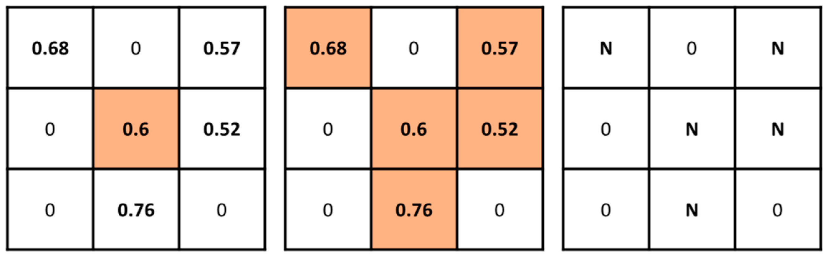
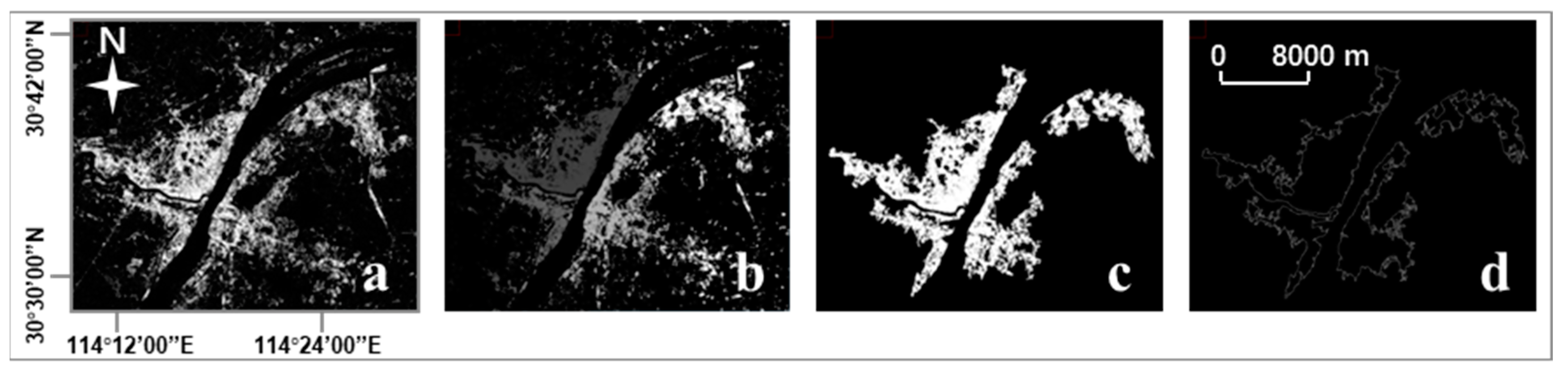
Corresponding to the definition of urban area in this paper, the urban area could be generated based on the high-density ISA images. Referring to previous research [71,74], the ISA fractions greater than 0.5 would be assigned as high-density ISA. Firstly, aggregation was applied on the ISA image. For each target pixel, searching in its eight-neighborhood, the target pixel and its neighborhood pixels whose ISA fraction was greater than 0.5 (i.e., high-density) were assigned as the same value (Figure 4), which was a similar approach to the City Clustering Algorithm (CCA) [74,75,76]. The search was undertaken until all the pixels were tested, after which an indexed map could be generated with a unique index for each aggregated area (Figure 5b). Secondly, with the help of the high-resolution images, the aggregated areas corresponding to the urban core, built-up clusters in suburb and the new districts set up by the government (e.g., Tianjin Binhai New District) were extracted. For example, from satellite images, we were able to find that the urban core for Wuhan city was located alongside the Yangtze River. Thus, the indexes for aggregated areas corresponding to the urban core could easily be found by visual interpretation. With those indexes extracted, the urban area could be picked up from Figure 3b,c by attribute extraction. Finally, the boundary of the aggregated built-up area was generated (Figure 5d). The areas within the boundary were assigned as the urban area, including all the impervious and pervious surfaces except water bodies.
Since all the impervious and pervious surfaces (water bodies excluded) within the urban boundary were marked as urban area, it could be pointed out that the land cover changes within the urban boundary would not affect the total area of urban extent. Thus, considering the progress of urbanization, we insisted the hypothesis that the urban area in a particular year would not be less than that in the former year. In practice, the urban area in this year can be expressed as the sum of the new urban area generated in this year and the urban area of the last year.
3. Results
3.1. Accuracy of Impervious Surface Area
The analysis for the 36 major cities were generally based on the ISA extracted in this paper. Thus, the spatial and temporal accuracy for ISA was required to be accurate and stable. Based on the aforementioned method of accuracy assessment, we were pleased to find that the extracted ISA was a series with stable accuracy.
In detail, from Table S4 (right part), taking Wuhan as the test area, there existed an average error of 0.05–0.07 for different years (0.05 for 2000; 0.07 for 2004; and 0.06 for 2013, average for three years: 0.06). Thus, the temporal consistency for the ISA was tested. For the spatial accuracy, we were able to find that the difference between estimated ISA abundance and true ISA abundance was mostly less than 0.1 with an average RMSE of 0.07 for all abundances (0.05–0.97, value interval circa 0.28) across all cities. As the spatial and temporal error level for ISA abundances was relatively low and stable, the value and temporal trends for the following extracted ISA and urban area were also acceptable.
3.2. Urban Expansion Rates and Modes
To qualify the urban expansion area and rates, by analyzing the three decades of satellite images, our results showed that almost all the cities experienced a dramatic expansion in this period. The urban area ratio (UAR) was calculated as the urban area in 2015 divided by the urban area in 1986. For those cities without clear images in 1986 or 2015, extrapolation or interpolation (for those cities with clear images before 1986 or after 2015) was used to obtain the urban area in 1986 or 2015. The UAR for all 36 cities was 5.85, and the expansion area was 15.51 km2 per city per year. In addition, many of the cities showed an average growth rate (AGR, Table 1) [36,41] of around 4–7%.
However, large variations in expansion area and AGR exist across China. For instance, Shenzhen (Figure 6b), as the “window” of China’s reform and opening-up, possesses the highest AGR (12.23%) and the largest UAR (31.88), living up to the title of “a city rising in a night”. Meanwhile, the lowest level of urban expansionwas found in Beijing (Figure 6a), with an AGR of 3.23% and an UAR of 2.59. This may be attributed to two reasons. Firstly, as the capital of China, Beijing had already developed to a relatively high level by the 1980s, and thus the available space for continued urban expansion was limited. Secondly, the stringent urban land policies in Beijing played an important role in restraining the rapid expansion.
As for the expansion area (Figure 7), Shanghai tops the list, with 1716.03 km2 taken up by urban expansion. For one thing, the original urban area in Shanghai was large. For another thing, the Pudong district, which developed from the late 20th century and is regarded as the second national new district after Shenzhen, promoted the urban expansion in Shanghai. Meanwhile, Lhasa, restricted by natural conditions, shows the smallest increase in urban extent, with only 96.42 km2 taken up by urban expansion. Overall, China has experienced dramatic urban expansion; however, influenced by a development basis, government policies, and natural conditions, the urban expansion shows great heterogeneity across cities.
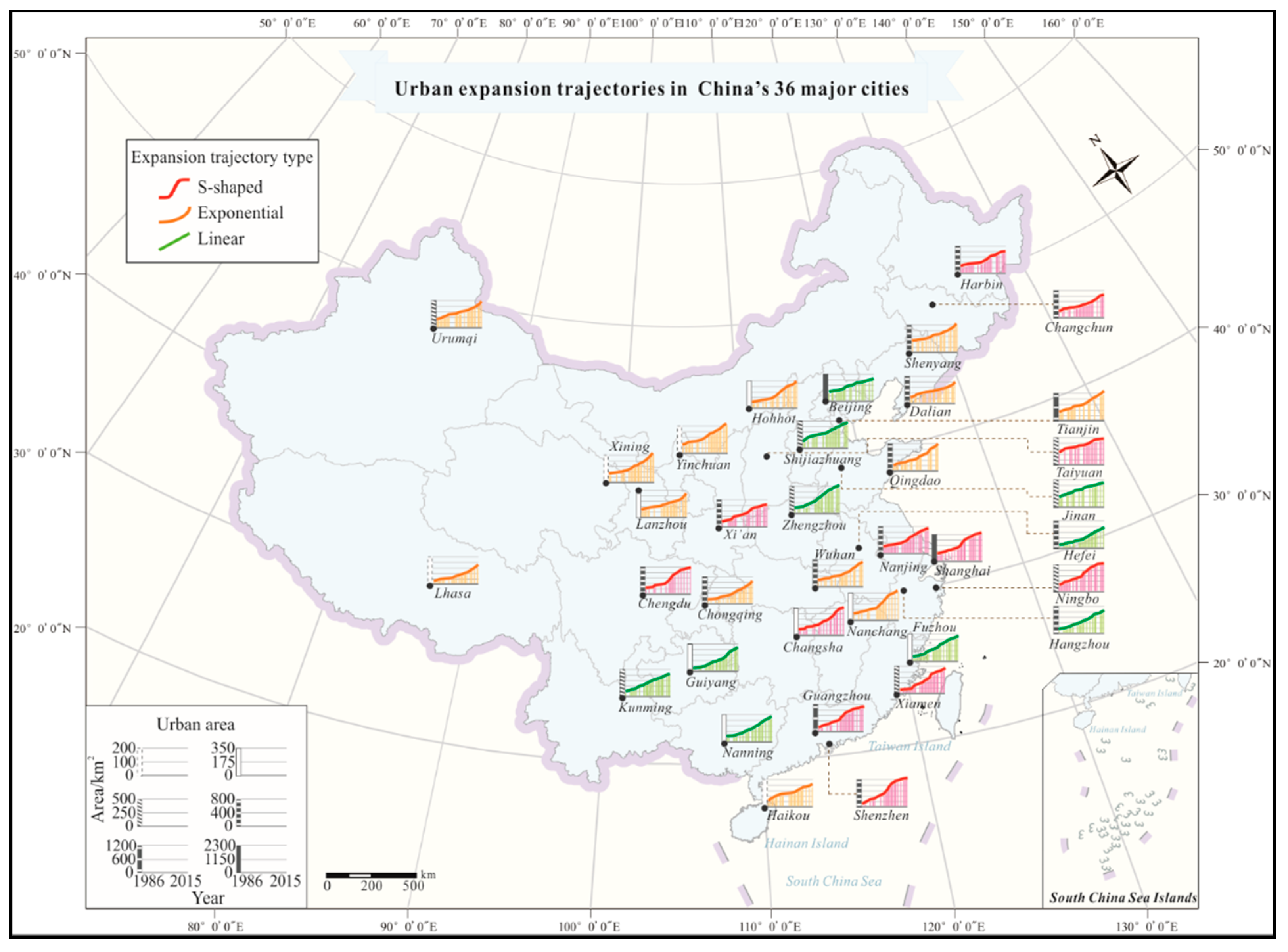
To further explore the expansion patterns for different cities, a map illustrating the urban expansion trajectories is provided in Figure 8. For the city areas generated in the different study years, a linear function (linear expansion), exponential function (exponential expansion), and logistic function (s-shaped expansion) were applied to fit the regression. The result obtaining the highest R2 was chosen as the adapted curve for the expansion trajectory. Thus, there were three patterns for urban expansion: (1) exponential expansion (14 cities); (2) expansion (10 cities); and (3) s-shaped expansion (12 cities). Exponential expansion indicates that the urban growth rate increased significantly in recent years; linear expansion indicates a relatively stable development pace; and s-shaped expansion can be explained as a city experiencing an initial slow growth followed by a rapid growth finally turning into a stage with slower development. It should be noted that, in the literature, the urbanization curve is generally based on the urban population, and the s-shaped curve has attracted the most attention. Although the urban expansion curve in this research was generated by urban area, it is able to present similar information.
Interestingly, there are some connections between the growth patterns and the cities’ comprehensive competitiveness. Referring to the report in 2016 by China Business News Weekly, the 36 major cities were classified into five levels: first-tier cities, new first-tier cities, second-tier cities, third-tier cities, and fourth-tier cities (Figure 7). From Figure 8, it can be seen that all the third-tier and fourth-tier cities correspond to exponential expansion, suggesting that the development level of these cities is lower as they are still in the rapid expansion stage. All the first-tier cities, except for Beijing, have experienced s-shaped expansion, indicating that these cities tend to hold a stable urban layout after high-speed development, so that the urban growth rate then slows down. Differing from the cities mentioned above, the urban expansion trajectories for the new first-tier and second-tier cities present three patterns. Specifically, most of the second-tier cities show a linear expansion trend, demonstrating that the development of these cities has been relatively steady, without undergoing high-speed expansion. Half of the new first-tier cities have experienced rapid development in recent years, especially for those cities where new districts have been constructed, such as Tianjin Binhai New District and Qingdao Huangdao District. It can therefore be recognized that urban planning policies can greatly affect development progress.
3.3. Impervious Surface Variation in the Old City Zone
The urban expansion rates and modes lend support to the urban expansion laws, while the corresponding internal evolution laws remain unknown. To better describe the variation inside the urban area, we defined the urban area in the first study year as the target old city zone, and we tried to explain the internal structure variation in this zone by ISA change.
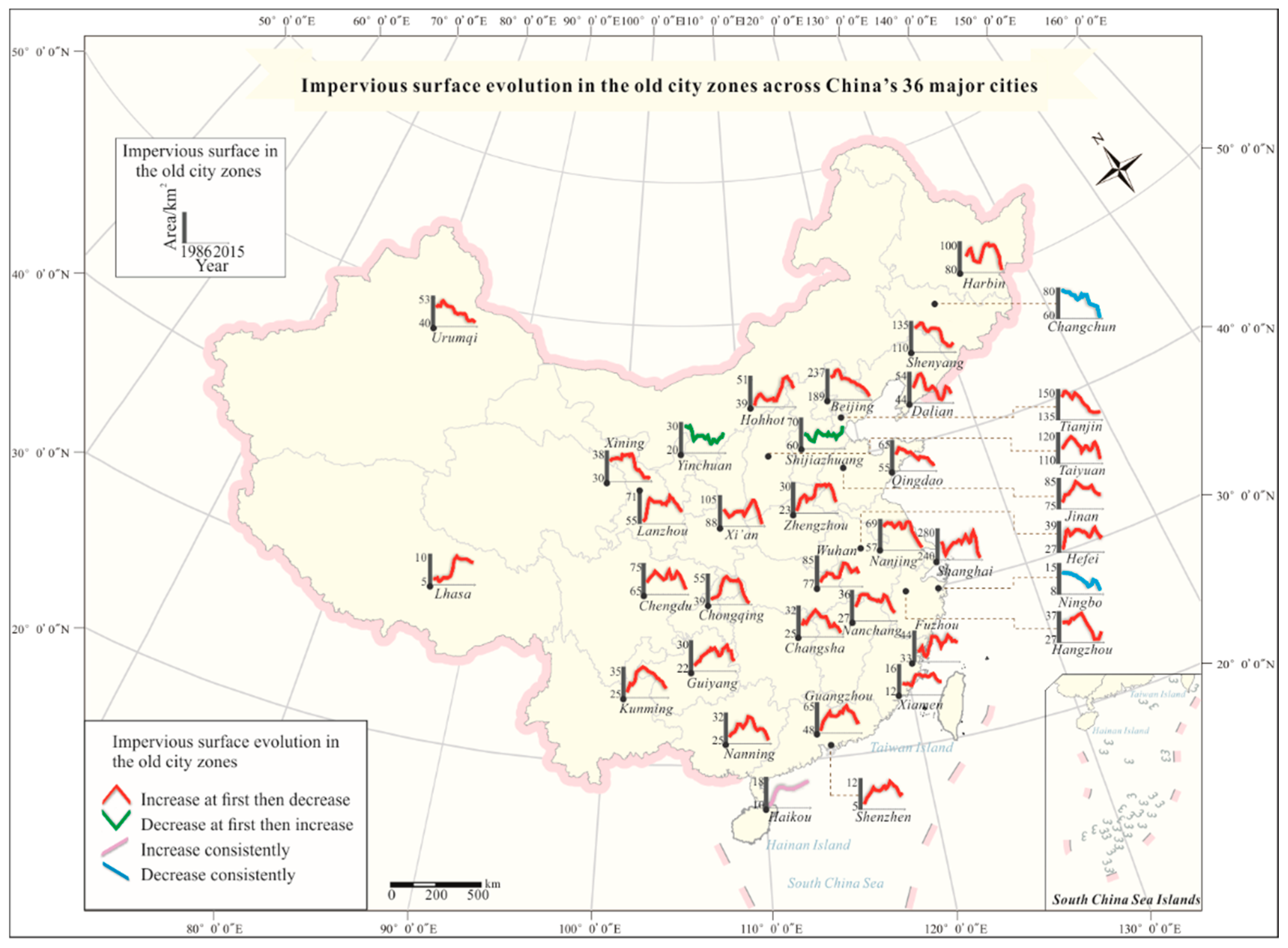
We mapped the evolution of ISA in the old city zones of 36 major cities during the past three decades (Figure 9), and an interesting trend was found: 31 cities showed the tendency of ISA first increasing and then decreasing. In general, natural land is converted into built-up land, corresponding to the progress of urbanization, so it is easy to understand the initial increase of ISA. However, how can we explain the subsequent decrease in ISA? This phenomenon may be rooted in the widespread demolition of old buildings. In China’s cities, a common phenomenon is to dismantle narrow built-up areas to build new housing estates or parks with high greening rates, resulting in a decrease of the ISA. Another major factor accounting for this phenomenon may be the reconstruction of urban villages. Urban villages are considered as a product of the traditional urban-rural dual system. Specifically, the rural land belongs to “collective ownership”, while urban land belongs to “national ownership”. Thus, the profit-oriented land expropriation policies initiated during city development tend to absorb farmland instead of rural residential areas, resulting in rural areas becoming surrounded by an urban area, which is a phenomenon that is known as the “urban village”. These areas are likely to be unregulated, so that the land distribution in these areas is commonly unreasonable with compact houses, narrow roads, and limited green lands (Figure 10a,c), greatly affecting the internal layout in an urban area. Therefore, the reconstruction of urban villages is aimed at adjusting the land structure, especially dismantling and reconstructing compact buildings. In addition, affected by the poor quality of the construction and unreasonable real estate development, buildings in an urban area generally show a short life cycle. It has been reported that the average building life cycle in China is only 30 years [77]. Large parts of demolished areas are transformed into modern communities (Figure 8a,b) and the other parts are transformed into public places (Figure 10c,d), because of the increasing need for an improved living environment. All these factors lead to the decrease of ISA in the old city zone.
Except for the trend of first increasing and then decreasing, there are also some other evolution trends for the ISA in a few cities. The ISA in the old city zones of Ningbo and Changchun present a trend of steady decrease. The reason why these cities did not show an initial stage of increasing ISA may be that the built-up areas in the old city zone of the two cities were relatively saturated by 1986. The trend in Shijiazhuang and Yinchuan was an initial slight decrease followed by an increase. Compared with the aforementioned cities, the increasing trend in recent years has been significant, which is probably attributable to government decisions. For Shijiazhuang, the increasing trend may be a result of the “great changes within three years” policy that has been enacted since 2007. For Yinchuan, the reason for the increasing trend may be the series of giant building projects undertaken since 2008 (e.g., Ningxia Software Park). The increasing trend of ISA in the two cities indicates that the city construction in recent years has taken place in undeveloped areas or green land. In particular, Haikou is the only city that has shown a tendency for consistent increase. As a capital city that was set up in 1988, Haikou’s foundation has been limited by the municipal facilities. As a result, a great deal of bare land in the old city zone has been converted into ISA during the urbanization progress, and the ISA has not yet reached a state of complete saturation in the old city zone.
3.4. Urban Expansion Interaction with Economy and Population
It has been reported that urban expansion is highly correlated with the economy and population growth [44,78,79,80,81,82]. In this research, we conducted a regression analysis using Gross Domestic Product (GDP) per capita (GDPPC) to represent the economy, and total population at the year-end (TP) for the population. The Ordinary Least Square (OLS) regressions between ISA and GDPPC, and between ISA and TP showed that the determination coefficients (R2) for most cities were greater than 0.9 (Table S2). The smallest determination coefficients were greater than 0.84 (for GDPPC) and 0.69 (for TP), verifying the high correlation between urban expansion and economy, and between urban expansion and population in China’s cities. To further reveal the interaction, the potential driving mechanism was investigated with the help of GCT [59,83,84] (Supplementary Information Text S3). Since the ISA used in this paper were not time-continuous, a regression between the year and the ISA was conducted to obtain the probable ISA in missing years. In detail, the ISA variation was fitted by linear, exponential and s-shaped functions, and the best fitting function was selected. Thus, the interpolation could be carried out following the selected function and a time-continuous series of ISA could be gained. Next, the Augmented Dickey–Fuller (ADF) test was applied to the time-continuous series of ISA, GDPPC, and TP. Co-integration was found in all cities except for Kunming by the Johansen co-integration test. Therefore, the GCT was applied to 35 (Kunming excluded) of the 36 cities. Furthermore, since the Granger causality result may not be the same among different lag orders, the result with the optimal lag order (verified by the Akaike information criterion and the Schwarz information criterion) was chosen. If there was no granger causality when using the optimal lag order, the result found in most of the lag orders was chosen. Based on the GCT, if event A “Granger-causes” event B, event A is taken as a potential driver.
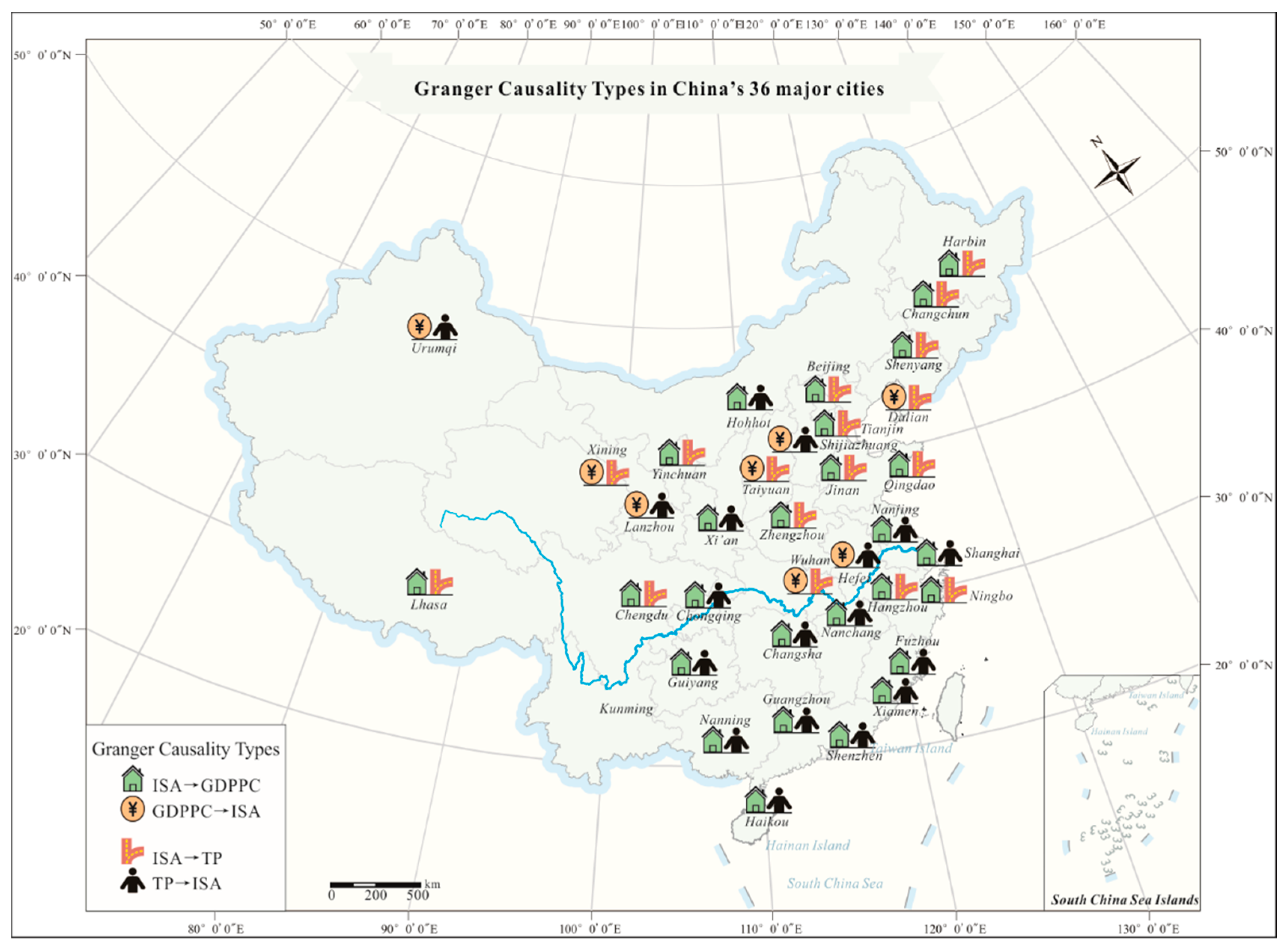
From the GCT in the 35 cities (Table S3; Figure 11), there existed an obvious north-south differentiation for the interaction between ISA and TP. Taking the Yangtze River as the division between north and south China, most of the cities in the south indicated that TP Granger-causes ISA. Meanwhile, in the north, most of the cities indicated that ISA Granger-causes TP. A possible explanation for this may be that, for the south, it is a rapidly developed zone that has benefited from earlier reform and opening-up. Therefore, a number of young adults are continually being attracted to seek work opportunities in the south, bringing new vigor and vitality into the urban construction. As a result, the population has become the major driver of the southern cities’ development. An exception is the Zhejiang province, where many people are willing to travel for business, likely resulting in ISA Granger-causing TP for Hangzhou and Ningbo. For the north, in contrast, the opening-up took place later. Thus, many people in the north have rushed to the south for work opportunities. Hence, most of the northern cities should conduct urban construction first, then attract the backflow of population. ISA has therefore become the major driver of the northern cities’ development.
For the interaction between ISA and GDPPC (Table S3; Figure 11), the majority of the cities (27 cities) indicated that ISA Granger-causes GDPPC, confirming that the economic growth in China’s cities has been greatly dependent on ISA expansion in the past three decades [85,86,87]. It is frustrating that some cities in China have expanded blindly to pursue economic growth. In particular, the GDP growth is heavily reliant on real estate in some cities, resulting in wild urban space expansion, bringing some negative effects. To solve these problems, the government has promulgated policies for controlling urban size since 2013 (“National Plan on New Urbanization 2014–2020”). As expected, only a few cities (eight cities) indicated that GDPPC Granger-causes ISA. All these cities are located to the north of the Yangtze River. Supported by resource superiority (Dalian, Taiyuan, Urumqi) or policy investment (Shijiazhuang, Lanzhou, Xining, Wuhan, Hefei), the economic returns of these cities are mainly used for urban construction.
However, it should be recognized that GCT does not prove that one variable “causes” another except in the sense that it precedes the other in time. Even though one factor is likely to promote the other when one factor happened earlier than the other, in the future, more concerns about land requisitions and government policies should be involved to assist the GCT results in pointingto a more “real” causality.
4. Discussion
4.1. The Differences in Urban Expansion Trajectories
In our study, we found three different growth patterns for urban expansion in China, i.e., s-shaped, linear, and exponential. According to the current research, some researchers insist that the s-shaped curve is more suitable for developed countries [88,89], while a j-shaped curve (similar to the exponential curve) is more appropriate for developing countries [90]. However, our results have indicated that great heterogeneity exists for urban expansion trajectories, even in the same country.
Moreover, although the urban expansion trajectories are relatively uniformed for cities in the same development level, there are still some exceptions. For example, as a first-tier city, Beijing demonstrates a linear expansion trend rather than a s-shaped trend because it developed in much earlier years and might have reached a stable development stage in the 1980s. Haikou and Urumqi, as the cities list at the end of second-tier cities, present urban expansion trajectories more similar with third-tier cities, i.e., exponential growth. We can therefore recognize that those cities also need rapid urban expansion to develop themselves. In addition, Chengdu as the top city of new first-tier cities, shows a similar s-shaped trend of urban expansion trajectory with first-tier cities. We can also infer that the urban growth in Chengdu has reached a stable stage, and it may get closer to the development of first-tier cities in the future.
In general, a fact emerged that both linear and exponential trends represented initial stages of s-shaped growth. In other words, for those cities without a s-shaped trend, we suggested that they would turn into a s-shaped development in the future. In reverse, for a city in China, when its growth pattern was figured out (exponential, linear or s-shaped), we could roughly point out its current development level.
4.2. The Limitations of Our Work
Even though we have tried to take all aspects of the entire research matter into consideration, there are some limitations to our work. Firstly, on account of the effects of cloud cover and sensor malfunction, we could not obtain high-quality Landsat remote sensing images of 36 cities for all the years from 1986 to 2015. To solve this problem, we tried to recover the missing regions in the Landsat-7 images using a gap-filling method, and used temporal interpolation in the GCT test, which may have brought about some uncertainties which were difficult to quantify. Secondly, the population and GDP statistical data used in this paper were counted at the city level, but the ISA was computed on the main urban areas. Nevertheless, we considered this slight mismatch to be acceptable because the population and economic earnings were mostly concentrated in these areas. However, if district-level statistical data were available, the results would be more reliable. Thirdly, although the sub-pixel unmixing technique was used to extract the impervious surfaces, some bias inevitably exists. This is also one of the reasons for the small fluctuations in the impervious surface evolution for the old city zones shown in Figure 9. If the errors could be further reduced, we could make a more refined analysis of the urbanization progress by considering more influencing factors.
5. Conclusions
In this paper, we mapped and analyzed three decades of urban expansion in China’s 36 major cities. Both homogeneity and heterogeneity were established. With regard to homogeneity, almost all of China’s major cities have experienced rapid urban expansion. Meanwhile, a remarkable trend was found in the ISA variation in the city cores of the majority of China’s cities, i.e., ISA first increasing and then decreasing. This can be attributed to the urban development progress in China, especially the reconstruction of urban villages. Furthermore, the interaction between ISA and the economy tends to be ISA promoting the economy, confirming that the Chinese economy is highly dependent on urban expansion. In terms of heterogeneity, constrained by development basis, government policies, and natural conditions, the urban expansion trajectories show three modes: exponential, linear and s-shaped. Interestingly, there exists an obvious north-south territorial differentiation for the interaction between ISA and population. Cities in the north tend to indicate that ISA Granger-causes population, while cities in the south are more likely to indicate that population Granger-causes ISA. This phenomenon is in accordance with the fact that a lot of young adults from the north seek work opportunities in the south.
The results suggested that the policies issued by both central and local government have had a great impact on the progress of urbanization in China [58,85]. For instance, since Shenzhen was set up as a special economic zone in 1980, it has changed from a small fishing village into an international metropolis, with a GDP that transcends that of Hong Kong. Furthermore, since the Pudong New District was developed in 1990, economic efficiency has increased 118 times in 2014 compared to the initial period. In 2017, the central government decided to develop Xiong’an New District and tried to build it into a national new district after Shenzhen and Pudong, aiming to create a new era for reform and opening-up. The positive effects exerted by the national planning of new districts have been practically validated. However, excessively pursuing local GDP growth in some local policies has resulted in some blind expansion for new district development, which brings about not only traditional “city diseases”, but also some new negative effects. For example, some uninhabited new district, the so-called “ghost towns”, have resulted in a great waste of resources. In addition, the fact that economic earnings and government receipts depend more on real estate may lead to weak growth in the subsequent development. Even so, “creating another new town” is still the development goal of many cities. To deal with these problems, the central government has introduced policies (e.g., “New Urbanization Planning” in 2014 [91]) to strictly control urban size. Accordingly, local government should abandon the blind pursuit of political achievement and actively adjust city development strategies, insisting on sustainable development.
Supplementary Materials
The following are available online at https://www.mdpi.com/2072-4292/12/3/491/s1, Text S1: Endmember selection for linear spectral mixture analysis, Text S2: Sample selection for accuracy assessment, Text S3: Granger causality test, Table S1: Landsat data used in this research, Table S2: Regression results between ISA and GDPPC, and also between ISA and TP, Table S3: Granger causality results, Table S4: Accuracy assessment for impervious surface.
Author Contributions
Conceptualization, H.S. and L.Z.; methodology, H.S. and Y.S.; validation, H.S. and Y.S.; formal analysis, H.S. and Y.S.; investigation, H.S. and Y.S.; resources, H.S., L.Z., Q.C. and Y.S.; data curation, H.S., L.Z., Q.C., L.H. and Y.S.; writing—original draft preparation, H.S., Q.C. and Y.S.; writing—review and editing, H.S., Q.C. and Y.S.; visualization, Y.S.; supervision, H.S., L.Z. and Q.C.; project administration, H.S. and L.Z.; funding acquisition, H.S. All authors have read and agreed to the published version of the manuscript.
Funding
This research was funded by the National Natural Science Foundation of China, grant number 41422108; and the Youth Talent Support Program of China (2015).
Acknowledgments
We would like to thank the data providers of the USGS Earth Resources Observation and Science (EROS) Center and China’s National Bureau of Statistics. We would also like to thank Ying Song and Lina Huang for assistance with the mapping, and Zengxiang Zhang (working in the Institute of Remote Sensing and Digital Earth of Chinese Academy of Sciences) for kindly providing us with an atlas expressing urban expansion.
Conflicts of Interest
The authors declare no conflicts of interest.
References
- Turner, B.L., II; Lambin, E.F.; Reenberg, A. The emergence of land change science for global environmental change and sustainability. Proc. Natl. Acad. Sci. USA 2007, 104, 20666–20671. [Google Scholar] [CrossRef] [Green Version]
- Bierwagen, B.G.; Theobald, D.M.; Pyke, C.R.; Choate, A.; Groth, P.; Thomas, J.V.; Morefield, P. National housing and impervious surface scenarios for integrated climate impact assessments. Proc. Natl. Acad. Sci. USA 2010, 107, 20887–20892. [Google Scholar] [CrossRef] [Green Version]
- Cohen, B. Urban growth in developing countries: A review of current trends and a caution regarding existing forecasts. World Dev. 2004, 32, 23–51. [Google Scholar] [CrossRef]
- Grimm, N.B.; Faeth, S.H.; Golubiewski, N.E.; Redman, C.L.; Wu, J.; Bai, X.; Briggs, J.M. Global change and the ecology of cities. Science 2008, 319, 756–760. [Google Scholar] [CrossRef] [Green Version]
- Huang, X.; Xia, J.; Xiao, R.; He, T. Urban expansion patterns of 291 chinese cities, 1990–2015. Int. J. Digit. Earth 2017, 1–16. [Google Scholar] [CrossRef]
- Seto, K.C.; Guneralp, B.; Hutyra, L.R. Global forecasts of urban expansion to 2030 and direct impacts on biodiversity and carbon pools. Proc. Natl. Acad. Sci. USA 2012, 109, 16083–16088. [Google Scholar] [CrossRef] [Green Version]
- Bloom, D.E.; Canning, D.; Fink, G. Urbanization and the wealth of nations. Science 2008, 319, 772. [Google Scholar] [CrossRef] [Green Version]
- Newbold, T.; Hudson, L.N.; Hill, S.L.; Contu, S.; Lysenko, I.; Senior, R.A.; Borger, L.; Bennett, D.J.; Choimes, A.; Collen, B.; et al. Global effects of land use on local terrestrial biodiversity. Nature 2015, 520, 45–50. [Google Scholar] [CrossRef] [Green Version]
- Hahs, A.K.; McDonnell, M.J.; McCarthy, M.A.; Vesk, P.A.; Corlett, R.T.; Norton, B.A.; Clemants, S.E.; Duncan, R.P.; Thompson, K.; Schwartz, M.W. A global synthesis of plant extinction rates in urban areas. Ecol. Lett. 2009, 12, 1165–1173. [Google Scholar] [CrossRef]
- Zuo, L.; Zhang, Z.; Carlson, K.M.; MacDonald, G.K.; Brauman, K.A.; Liu, Y.; Zhang, W.; Zhang, H.; Wu, W.; Zhao, X.; et al. Progress towards sustainable intensification in china challenged by land-use change. Nat. Sustain. 2018, 1, 304–313. [Google Scholar] [CrossRef]
- Li, J.; Song, C.; Cao, L.; Zhu, F.; Meng, X.; Wu, J. Impacts of landscape structure on surface urban heat islands: A case study of shanghai, china. Remote Sens. Environ. 2011, 115, 3249–3263. [Google Scholar] [CrossRef]
- Schneider, A.; Friedl, M.A.; Potere, D. A new map of global urban extent from modis satellite data. Environ.Res. Lett. 2009, 4, 044003. [Google Scholar] [CrossRef] [Green Version]
- Schneider, A.; Friedl, M.A.; Potere, D. Mapping global urban areas using modis 500-m data: New methods and datasets based on ‘urban ecoregions’. Remote Sens. Environ. 2010, 114, 1733–1746. [Google Scholar] [CrossRef]
- Wang, J.; Zhao, Y.; Li, C.; Yu, L.; Liu, D.; Gong, P. Mapping global land cover in 2001 and 2010 with spatial-temporal consistency at 250 m resolution. ISPRS-J. Photogramm. Remote Sens. 2015, 103, 38–47. [Google Scholar] [CrossRef]
- Zhang, Q.; Seto, K.C. Mapping urbanization dynamics at regional and global scales using multi-temporal dmsp/ols nighttime light data. Remote Sens. Environ. 2011, 115, 2320–2329. [Google Scholar] [CrossRef]
- Small, C.; Pozzi, F.; Elvidge, C.D. Spatial analysis of global urban extent from dmsp-ols night lights. Remote Sens. Environ. 2005, 96, 277–291. [Google Scholar] [CrossRef]
- Zhou, Y.; Steven, J.S.; Zhao, K.; Marc, I.; Allison, T.; Ben, B.-L.; Ghassem, R.A.; Zhang, X.; He, C.; Christopher, D.E. A global map of urban extent from nightlights. Environ. Res. Lett. 2015, 10, 054011. [Google Scholar] [CrossRef]
- Bagan, H.; Yamagata, Y. Land-cover change analysis in 50 global cities by using a combination of landsat data and analysis of grid cells. Environ. Res. Lett. 2014, 9, 064015. [Google Scholar] [CrossRef]
- Chen, J.; Chen, J.; Liao, A.; Cao, X.; Chen, L.; Chen, X.; He, C.; Han, G.; Peng, S.; Lu, M.; et al. Global land cover mapping at 30 m resolution: A pok-based operational approach. ISPRS-J. Photogramm. Remote Sens. 2015, 103, 7–27. [Google Scholar] [CrossRef] [Green Version]
- Liu, X.; Hu, G.; Chen, Y.; Li, X.; Xu, X.; Li, S.; Pei, F.; Wang, S. High-resolution multi-temporal mapping of global urban land using landsat images based on the google earth engine platform. Remote Sens. Environ. 2018, 209, 227–239. [Google Scholar] [CrossRef]
- Zhou, Y.; Smith, S.J.; Elvidge, C.D.; Zhao, K.; Thomson, A.; Imhoff, M. A cluster-based method to map urban area from dmsp/ols nightlights. Remote Sens. Environ. 2014, 147, 173–185. [Google Scholar] [CrossRef]
- Hu, L.; Brunsell, N.A. A new perspective to assess the urban heat island through remotely sensed atmospheric profiles. Remote Sens. Environ. 2015, 158, 393–406. [Google Scholar] [CrossRef]
- Li, Q.; Lu, L.; Weng, Q.; Xie, Y.; Guo, H. Monitoring urban dynamics in the southeast u.S.A. Using time-series dmsp/ols nightlight imagery. Remote Sens. 2016, 8, 578. [Google Scholar] [CrossRef] [Green Version]
- Schneider, A.; Mertes, C.M.; Tatem, A.J.; Tan, B.; Sulla-Menashe, D.; Graves, S.J.; Patel, N.N.; Horton, J.A.; Gaughan, A.E.; Rollo, J.T.; et al. A new urban landscape in east–southeast asia, 2000–2010. Environ. Res. Lett. 2015, 10, 034002. [Google Scholar] [CrossRef]
- Tran, H.; Uchihama, D.; Ochi, S.; Yasuoka, Y. Assessment with satellite data of the urban heat island effects in asian mega cities. Int. J. Appl. Earth Obs. 2006, 8, 34–48. [Google Scholar] [CrossRef]
- Miettinen, J.; Shi, C.; Tan, W.J.; Liew, S.C. 2010 land cover map of insular southeast asia in 250-m spatial resolution. Remote Sens. Lett. 2012, 3, 11–20. [Google Scholar] [CrossRef]
- Kasanko, M.; Barredo, J.I.; Lavalle, C.; McCormick, N.; Demicheli, L.; Sagris, V.; Brezger, A. Are european cities becoming dispersed?: A comparative analysis of 15 european urban areas. Landscape Urban. Plan. 2006, 77, 111–130. [Google Scholar] [CrossRef]
- Antrop, M. Landscape change and the urbanization process in europe. Landscape Urban. Plan. 2004, 67, 9–26. [Google Scholar] [CrossRef]
- Mucher, C.A.; Steinnocher, K.T.; Kressler, F.P.; Heunks, C. Land cover characterization and change detection for environmental monitoring of pan-europe. Int. J. Remote Sens. 2000, 21, 1159–1181. [Google Scholar] [CrossRef]
- Brink, A.B.; Eva, H.D. Monitoring 25 years of land cover change dynamics in africa: A sample based remote sensing approach. Appl. Geogr. 2009, 29, 501–512. [Google Scholar] [CrossRef]
- Linard, C.; Tatem, A.J.; Gilbert, M. Modelling spatial patterns of urban growth in africa. Appl. Geogr. 2013, 44, 23–32. [Google Scholar] [CrossRef]
- Kuijs, L.; Wang, T. China’s pattern of growth: Moving to sustainability and reducing inequality. China World Econ. 2006, 14, 1–14. [Google Scholar] [CrossRef]
- Anderson, G.; Ge, Y. Do economic reforms accelerate urban growth? The case of china. Urban. Stud. 2016, 41, 2197–2210. [Google Scholar] [CrossRef]
- Seto, K.C.; Sánchez-Rodríguez, R.; Fragkias, M. The new geography of contemporary urbanization and the environment. Annu. Rev. Environ. Resour. 2010, 35, 167–194. [Google Scholar] [CrossRef] [Green Version]
- Tan, M. Urban land expansion and arable land loss of the major cities in china in the 1990s. Sci. China Ser. D 2005, 48, 1492. [Google Scholar] [CrossRef]
- Seto, K.C.; Fragkias, M.; Güneralp, B.; Reilly, M.K. A meta-analysis of global urban land expansion. PLoS ONE 2011, 6, e23777. [Google Scholar] [CrossRef]
- Schneider, A.; Mertes, C.M. Expansion and growth in chinese cities, 1978–2010. Environ. Res. Lett. 2014, 9, 024008. [Google Scholar] [CrossRef]
- Haas, J.; Ban, Y. Urban growth and environmental impacts in jing-jin-ji, the yangtze, river delta and the pearl river delta. Int. J. Appl. Earth Obs. 2014, 30, 42–55. [Google Scholar] [CrossRef]
- Wang, L.; Li, C.; Ying, Q.; Cheng, X.; Wang, X.; Li, X.; Hu, L.; Liang, L.; Yu, L.; Huang, H.; et al. China’s urban expansion from 1990 to 2010 determined with satellite remote sensing. Chin. Sci. Bull. 2012, 2802–2812, 2947–2950. [Google Scholar] [CrossRef] [Green Version]
- Xu, X.; Min, X. Quantifying spatiotemporal patterns of urban expansion in china using remote sensing data. Cities 2013, 35, 104–113. [Google Scholar] [CrossRef]
- Zhao, S.; Zhou, D.; Zhu, C.; Qu, W.; Zhao, J.; Sun, Y.; Huang, D.; Wu, W.; Liu, S. Rates and patterns of urban expansion in china’s 32 major cities over the past three decades. Landscape Ecol. 2015, 30, 1541–1559. [Google Scholar] [CrossRef]
- Zhao, S.; Zhou, D.; Zhu, C.; Sun, Y.; Wu, W.; Liu, S. Spatial and temporal dimensions of urban expansion in china. Environ. Sci. Technol. 2015, 49, 9600–9609. [Google Scholar] [CrossRef]
- Kuang, W.; Liu, J.; Dong, J.; Chi, W.; Zhang, C. The rapid and massive urban and industrial land expansions in china between 1990 and 2010: A clud-based analysis of their trajectories, patterns, and drivers. Landscape Urban. Plan. 2016, 145, 21–33. [Google Scholar] [CrossRef]
- Deng, X.; Huang, J.; Rozelle, S.; Uchida, E. Growth, population and industrialization, and urban land expansion of china. J. Urban. Econ. 2008, 63, 96–115. [Google Scholar] [CrossRef]
- Liu, J.; Zhan, J.; Deng, X. Spatio-temporal patterns and driving forces of urban land expansion in china during the economic reform era. Ambio 2005, 34, 450–455. [Google Scholar] [CrossRef]
- Fang, C.; Li, G.; Wang, S. Changing and differentiated urban landscape in china: Spatiotemporal patterns and driving forces. Environ. Sci. Technol. 2016, 50, 2217–2227. [Google Scholar] [CrossRef]
- Yang, X.; Ruby Leung, L.; Zhao, N.; Zhao, C.; Qian, Y.; Hu, K.; Liu, X.; Chen, B. Contribution of urbanization to the increase of extreme heat events in an urban agglomeration in east china. Geophys. Res. Lett. 2017, 44, 6940–6950. [Google Scholar] [CrossRef]
- Zhong, S.; Qian, Y.; Sarangi, C.; Zhao, C.; Leung, R.; Wang, H.; Yan, H.; Yang, T.; Yang, B. Urbanization effect on winter haze in the yangtze river delta region of china. Geophys. Res. Lett. 2018, 45, 6710–6718. [Google Scholar] [CrossRef]
- Lin, X.; Wang, Y.; Wang, S.; Wang, D. Spatial differences and driving forces of land urbanization in China. J. Geogr. Sci. 2015, 25, 545–558. [Google Scholar] [CrossRef]
- Tan, M.; Li, X.; Xie, H.; Lu, C. Urban land expansion and arable land loss in china—A case study of beijing–tianjin–hebei region. Land Use Pol. 2005, 22, 187–196. [Google Scholar] [CrossRef]
- Traore, A.; Watanabe, T. Modeling determinants of urban growth in conakry, guinea: A spatial logistic approach. Urban. Sci. 2017, 1, 12. [Google Scholar] [CrossRef] [Green Version]
- Maimaitijiang, M.; Ghulam, A.; Sandoval, J.S.O.; Maimaitiyiming, M. Drivers of land cover and land use changes in st. Louis metropolitan area over the past 40 years characterized by remote sensing and census population data. Int. J. Appl. Earth Obs. 2015, 35, 161–174. [Google Scholar] [CrossRef]
- Mustafa, A.M.; Cools, M.; Saadi, I.; Teller, J. Urban development as a continuum: A multinomial logistic regression approach. In Proceedings of the Computational Science and Its Applications—ICCSA 2015, Banff, AB, Canada, 22–25 June 2015; Gervasi, O., Murgante, B., Misra, S., Gavrilova, M.L., Rocha, A.M.A.C., Torre, C., Taniar, D., Apduhan, B.O., Eds.; Springer International Publishing: Cham, Switzerland, 2015; pp. 729–744. [Google Scholar]
- Mustafa, A.; Van Rompaey, A.; Cools, M.; Saadi, I.; Teller, J. Addressing the determinants of built-up expansion and densification processes at the regional scale. Urban. Stud. 2018, 55, 3279–3298. [Google Scholar] [CrossRef] [Green Version]
- Ma, Y.; Xu, R. Remote sensing monitoring and driving force analysis of urban expansion in guangzhou city, china. Habitat Int. 2010, 34, 228–235. [Google Scholar] [CrossRef]
- Lo, C.P. Urban indicators of china from radiance-calibrated digital dmsp-ols nighttime images. Ann. Assoc. Am. Geogr. 2010, 92, 225–240. [Google Scholar] [CrossRef]
- Deng, X.; Huang, J.; Scott, R.; Emi, U. Economic growth and the expansion of urban land in China. Urban. Stud. 2009, 47, 813–843. [Google Scholar] [CrossRef]
- Wen, Q.; Zhang, Z.; Shi, L.; Zhao, X.; Liu, F.; Xu, J.; Yi, L.; Liu, B.; Wang, X.; Zuo, L.; et al. Extraction of basic trends of urban expansion in china over past 40 years from satellite images. Chin. Geogr. Sci. 2016, 26, 129–142. [Google Scholar] [CrossRef] [Green Version]
- Bai, X.; Chen, J.; Shi, P. Landscape urbanization and economic growth in china: Positive feedbacks and sustainability dilemmas. Environ. Sci. Technol. 2012, 46, 132–139. [Google Scholar] [CrossRef]
- Song, S.; Zhang, K.H. Urbanisation and city size distribution in china. Urban. Stud. 2002, 39, 2317–2327. [Google Scholar] [CrossRef]
- Shen, H.; Li, X.; Cheng, Q.; Zeng, C.; Yang, G.; Li, H.; Zhang, L. Missing information reconstruction of remote sensing data: A technical review. IEEE Geosci. Remote Sens. Mater. 2015, 3, 61–85. [Google Scholar] [CrossRef]
- Shen, H.; Zhang, L. A map-based algorithm for destriping and inpainting of remotely sensed images. IEEE Trans. Geosci. Remote 2009, 47, 1492–1502. [Google Scholar] [CrossRef]
- Shen, H.; Huang, L.; Zhang, L.; Wu, P.; Zeng, C. Long-term and fine-scale satellite monitoring of the urban heat island effect by the fusion of multi-temporal and multi-sensor remote sensed data: A 26-year case study of the city of wuhan in china. Remote Sens. Environ. 2016, 172, 109–125. [Google Scholar] [CrossRef]
- Zeng, C.; Shen, H.; Zhang, L. Recovering missing pixels for landsat etm+ slc-off imagery using multi-temporal regression analysis and a regularization method. Remote Sens. Environ. 2013, 131, 182–194. [Google Scholar] [CrossRef]
- Wu, C. Normalized spectral mixture analysis for monitoring urban composition using etm+ imagery. Remote Sens. Environ. 2004, 93, 480–492. [Google Scholar] [CrossRef]
- McFeeters, S.K. The use of the normalized difference water index (ndwi) in the delineation of open water features. Int. J. Remote Sens. 1996, 17, 1425–1432. [Google Scholar] [CrossRef]
- Elvidge, C.; Tuttle, B.; Sutton, P.; Baugh, K.; Howard, A.; Milesi, C.; Bhaduri, B.; Nemani, R. Global distribution and density of constructed impervious surfaces. Sensors 2007, 7, 1962. [Google Scholar] [CrossRef]
- Imhoff, M.L.; Zhang, P.; Wolfe, R.E.; Bounoua, L. Remote sensing of the urban heat island effect across biomes in the continental USA. Remote Sens. Environ. 2010, 114, 504–513. [Google Scholar] [CrossRef] [Green Version]
- Zhang, P.; Imhoff, M.L.; Wolfe, R.E.; Bounoua, L. Characterizing urban heat islands of global settlements using modis and nighttime lights products. Can. J. Remote Sens. 2010, 36, 185–196. [Google Scholar] [CrossRef] [Green Version]
- Weng, Q.; Lu, D. A sub-pixel analysis of urbanization effect on land surface temperature and its interplay with impervious surface and vegetation coverage in indianapolis, united states. Int. J. Appl. Earth Obs. 2008, 10, 68–83. [Google Scholar] [CrossRef]
- Lu, D.; Weng, Q. Use of impervious surface in urban land-use classification. Remote Sens. Environ. 2006, 102, 146–160. [Google Scholar] [CrossRef]
- Wu, C.; Murray, A.T. Estimating impervious surface distribution by spectral mixture analysis. Remote Sens. Environ. 2003, 84, 493–505. [Google Scholar] [CrossRef]
- Shen, Y.; Shen, H.; Li, H.; Cheng, Q. Long-term urban impervious surface monitoring using spectral mixture analysis: A case study of Wuhan city in China. In Proceedings of the 2016 IEEE International Geoscience and Remote Sensing Symposium (IGARSS), Beijing, China, 10–15 July 2016; pp. 6754–6757. [Google Scholar]
- Peng, S.; Piao, S.; Ciais, P.; Friedlingstein, P.; Ottle, C.; Bréon, F.o.-M.; Nan, H.; Zhou, L.; Myneni, R.B. Surface urban heat island across 419 global big cities. Environ. Sci. Technol. 2011, 46, 696–703. [Google Scholar] [CrossRef]
- Rozenfeld, H.D.; Rybski, D.; Andrade, J.S.; Batty, M.; Stanley, H.E.; Makse, H.A. Laws of population growth. Proc. Natl. Acad. Sci. USA 2008, 105, 18702–18707. [Google Scholar] [CrossRef] [PubMed] [Green Version]
- Gong, P.; HOWARTH, P. The use of structural information for improving land-cover classification accuracies at the rural-urban fringe. Photogramm. Eng. Remote Sens. 1990, 56, 67–73. [Google Scholar]
- Qiu, B. Six fields with the largest building energy-saving potential and their outlooking in China (in Chinese). Archi Technol. 2011, 42, 6–8. [Google Scholar]
- Jiang, L.; Deng, X.; Seto, K.C. Multi-level modeling of urban expansion and cultivated land conversion for urban hotspot counties in China. Landscape Urban. Plan. 2012, 108, 131–139. [Google Scholar] [CrossRef]
- McGrath, D.T. More evidence on the spatial scale of cities. J. Urban. Econ. 2005, 58, 1–10. [Google Scholar] [CrossRef]
- Brueckner, J.K.; Fansler, D.A. The economics of urban sprawl: Theory and evidence on the spatial sizes of cities. Rev. Econ. Stat. 1983, 65, 479–482. [Google Scholar] [CrossRef]
- Bren d’Amour, C.; Reitsma, F.; Baiocchi, G.; Barthel, S.; Guneralp, B.; Erb, K.H.; Haberl, H.; Creutzig, F.; Seto, K.C. Future urban land expansion and implications for global croplands. Proc. Natl. Acad. Sci. USA 2017, 114, 8939–8944. [Google Scholar] [CrossRef] [Green Version]
- Luo, J.; Zhang, X.; Wu, Y.; Shen, J.; Shen, L.; Xing, X. Urban land expansion and the floating population in china: For production or for living? Cities 2018, 74, 219–228. [Google Scholar] [CrossRef]
- Granger, C.W.J. Investigating causal relations by econometric models and cross-spectral methods. Econometrica 1969, 37, 424–438. [Google Scholar] [CrossRef]
- Seto, K.C.; Kaufmann, R.K. Modeling the drivers of urban land use change in the pearl river delta, China: Integrating remote sensing with socioeconomic data. Land Econ. 2003, 79, 106–121. [Google Scholar] [CrossRef] [Green Version]
- Bai, X.; Shi, P.; Liu, Y. Realizing china’s urban dream. Nature 2014, 509, 158–160. [Google Scholar] [CrossRef] [Green Version]
- Ding, C.; Lichtenberg, E. Land and urban economic growth in china. J. Reg. Sci. 2011, 51, 299–317. [Google Scholar] [CrossRef]
- Lichtenberg, E.; Ding, C. Local officials as land developers: Urban spatial expansion in china. J. Urban. Econ. 2009, 66, 57–64. [Google Scholar] [CrossRef] [Green Version]
- Mulligan, G.F. Revisiting the urbanization curve. Cities 2013, 32, 113–122. [Google Scholar] [CrossRef]
- Chen, M.; Ye, C.; Zhou, Y. Comments on mulligan’s “revisiting the urbanization curve”. Cities 2014, 41, S54–S56. [Google Scholar] [CrossRef]
- Chen, Y. On the urbanization curves: Types, stages, and research methods. Sci. Geogr. Sin. 2012, 12–17. [Google Scholar]
- Zeng, C.; Zhang, M.; Cui, J.; He, S. Monitoring and modeling urban expansion—A spatially explicit and multi-scale perspective. Cities 2015, 43, 92–103. [Google Scholar] [CrossRef]
Figure 1.
Study area: China’s 36 major cities.

Figure 2.
An example of missing pixel recovery. (a) The reference image for Hefei on 16 May 2008. (b) The target image for Hefei on 27 July 2008. (c) The recovery result. (d) Magnified area for the red rectangle in (a). (e) Magnified area for the red rectangle in (b). (f) Magnified area for the red rectangle in (c).

Figure 3.
The 13 verification areas used for the accuracy assessment within the old city zone of Wuhan, China. The green rectangles indicate the target verification areas.
Figure 3.
The 13 verification areas used for the accuracy assessment within the old city zone of Wuhan, China. The green rectangles indicate the target verification areas.

Figure 4.
An example of impervious surface aggregation. The target pixel is highlighted in orange. When a target pixel is selected (the left image), a search is carried out within its eight-neighborhood until all the pixels greater than 0.5 are found (the middle image). Next, these pixels are assigned as the same number N. If this is the first search, then N would be 1; for the second search, N would be 2; and so forth.

Figure 5.
An example of urban boundary extraction in Wuhan on 11 August 1988. (a) Impervious surface image. (b) Aggregation image. (c) Impervious surface fitting with urban core area. (d) Urban boundary.
Figure 5.
An example of urban boundary extraction in Wuhan on 11 August 1988. (a) Impervious surface image. (b) Aggregation image. (c) Impervious surface fitting with urban core area. (d) Urban boundary.

Figure 6.
Urban area expansion in Beijing and Shenzhen.

Figure 7.
Urban area in China’s 36 major cities. The red bars are first-tier cities; the blue bars are new first-tier cities; the yellow bars are second-tier cities; the green bars are the third-tier cities; the purple bar is the fourth-tier cities. For each bar, the lower and darker color with slashes is the urban area in 1986, while the upper and lighter color is the urban area in 2015.
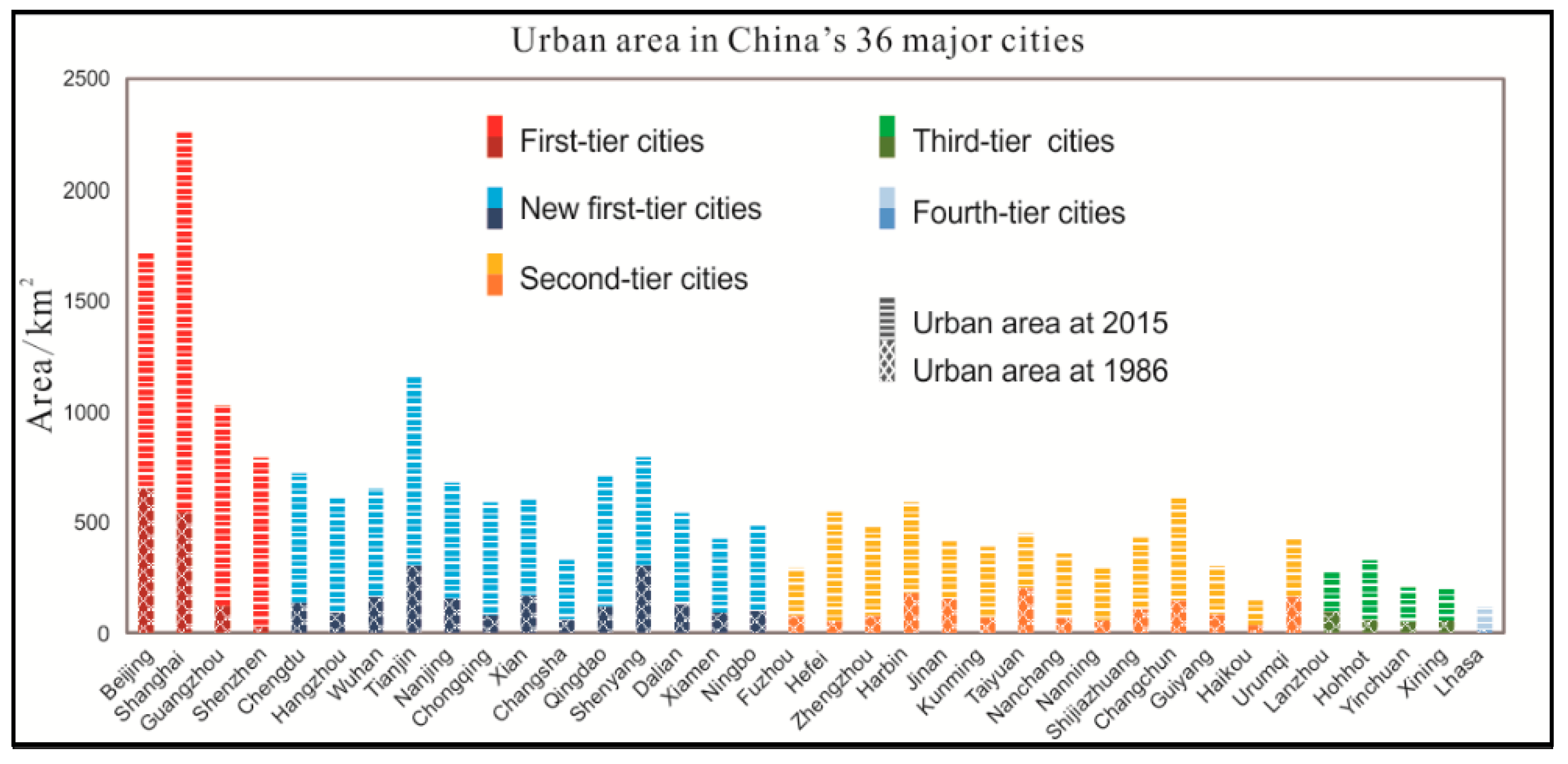
Figure 8.
Urban expansion trajectories in China’s 36 major cities from 1986 to 2015.

Figure 9.
Impervious surface evolution in the old city zones across China’s 36 major cities.

Figure 10.
Urban village construction in Wuhan and Beijing. (a) Wuhan Xudong business district on 1 November 2000. (b) Wuhan Xudong business district on 29 July 2016. (c) Beijing Olympic Village area on 28 January 2001. (d) Beijing Olympic Village area on 11 May 2017. Images are from Google Earth Pro 7.0. Significant changes can be seen within the red polygons (from (a) to (b) and from (c) to (d)).
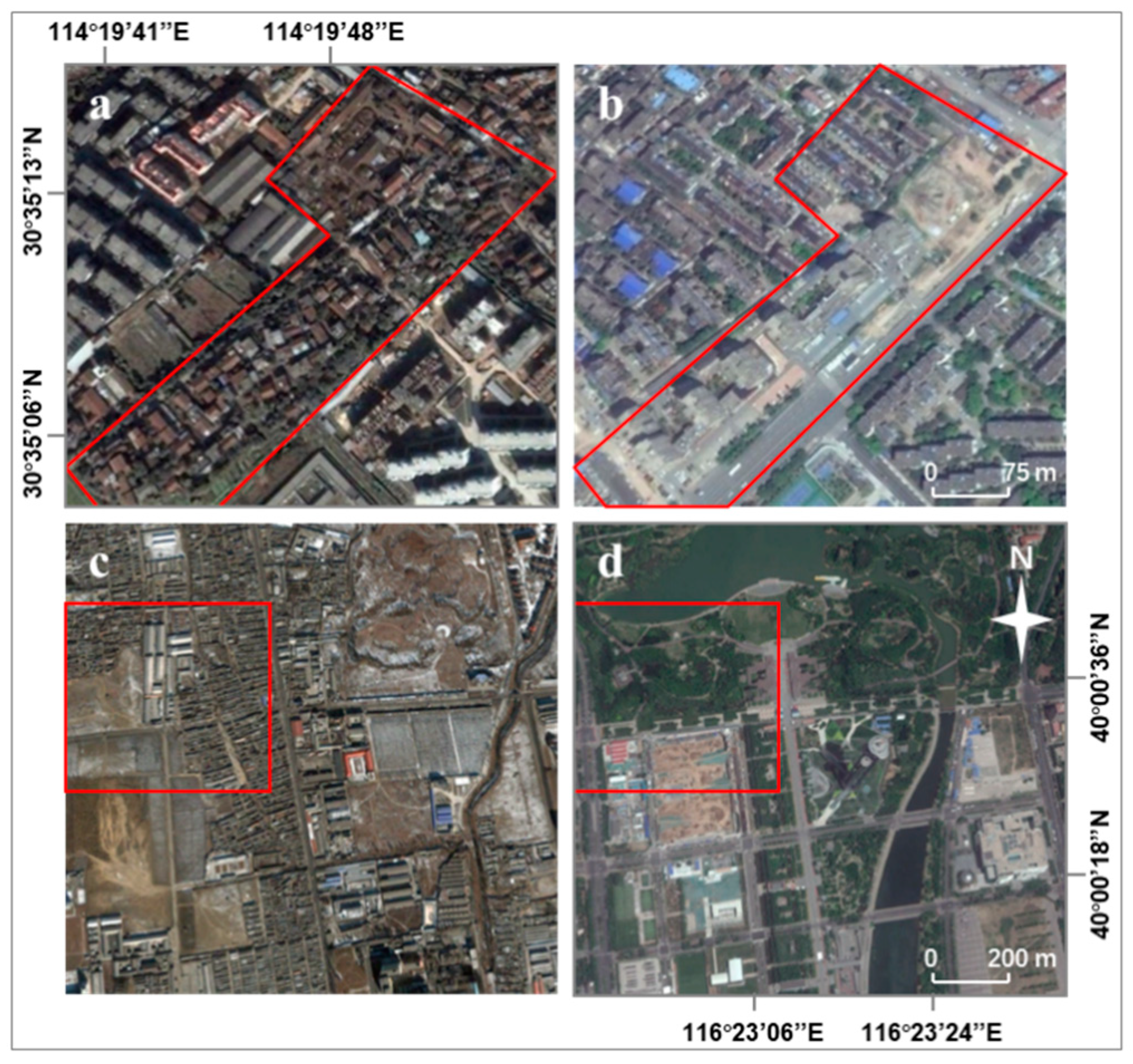
Figure 11.
Granger causality types in China’s 36 major cities. The blue line represents the Yangtze River.
Figure 11.
Granger causality types in China’s 36 major cities. The blue line represents the Yangtze River.


Table 1.
Average growth rate in China’s 36 major cities.
| Linear | Exponential | S-Shaped | ||||||
|---|---|---|---|---|---|---|---|---|
| Cities | AGR | UAR | Cities | AGR | UAR | Cities | AGR | UAR |
| Beijing | 3.23% | 2.59 | Wuhan | 4.76% | 4.03 | Shanghai | 4.86% | 4.15 |
| Hangzhou | 6.51% | 6.64 | Tianjin | 4.54% | 3.79 | Guangzhou | 6.35% | 8.44 |
| Fuzhou | 6.08% | 5.54 | Chongqing | 6.84% | 7.29 | Shenzhen | 12.23% | 31.88 |
| Hefei | 8.04% | 10.19 | Qingdao | 6.18% | 6.05 | Chengdu | 5.72% | 5.30 |
| Zhengzhou | 6.30% | 6.18 | Shenyang | 3.24% | 2.60 | Nanjing | 5.01% | 4.33 |
| Jinan | 3.32% | 2.67 | Dalian | 4.93% | 4.24 | Xi’an | 5.74% | 5.34 |
| Kunming | 5.91% | 5.60 | Nanchang | 5.73% | 5.98 | Changsha | 7.05% | 5.62 |
| Nanning | 5.77% | 5.38 | Haikou | 4.87% | 4.16 | Xiamen | 8.53% | 11.65 |
| Shijiazhuang | 4.71% | 3.98 | Urumqi | 3.89% | 3.14 | Ningbo | 5.44% | 4.91 |
| Guiyang | 6.08% | 5.54 | Lanzhou | 4.21% | 3.45 | Harbin | 4.05% | 3.29 |
| Hohhot | 5.93% | 5.62 | Taiyuan | 3.40% | 2.73 | |||
| Yinchuan | 4.70% | 3.96 | Changchun | 4.94% | 4.25 | |||
| Xining | 4.48% | 3.72 | ||||||
| Lhasa | 6.46% | 6.53 | ||||||
© 2020 by the authors. Licensee MDPI, Basel, Switzerland. This article is an open access article distributed under the terms and conditions of the Creative Commons Attribution (CC BY) license (http://creativecommons.org/licenses/by/4.0/).
Share and Cite
MDPI and ACS Style
Shen, Y.; Shen, H.; Cheng, Q.; Huang, L.; Zhang, L. Monitoring Three-Decade Expansion of China’s Major Cities Based on Satellite Remote Sensing Images. Remote Sens. 2020, 12, 491. https://doi.org/10.3390/rs12030491
AMA Style
Shen Y, Shen H, Cheng Q, Huang L, Zhang L. Monitoring Three-Decade Expansion of China’s Major Cities Based on Satellite Remote Sensing Images. Remote Sensing. 2020; 12(3):491. https://doi.org/10.3390/rs12030491
Chicago/Turabian StyleShen, Yao, Huanfeng Shen, Qing Cheng, Liwen Huang, and Liangpei Zhang. 2020. "Monitoring Three-Decade Expansion of China’s Major Cities Based on Satellite Remote Sensing Images" Remote Sensing 12, no. 3: 491. https://doi.org/10.3390/rs12030491
Note that from the first issue of 2016, this journal uses article numbers instead of page numbers. See further details here.