Abstract
The paper proposes a transparent approach for mapping the status of environmental phenomena from multisource information based on both soft computing and machine learning. It is transparent, intended as human understandable as far as the employed criteria, and both knowledge and data-driven. It exploits remote sensing experts’ interpretations to define the contributing factors from which partial evidence of the environmental status are computed by processing multispectral images. Furthermore, it computes an environmental status indicator (ESI) map by aggregating the partial evidence degrees through a learning mechanism, exploiting volunteered geographic information (VGI). The approach is capable of capturing the specificities of local context, as well as to cope with the subjectivity of experts’ interpretations. The proposal is applied to map the status of standing water areas (i.e., water bodies and rivers and human-driven or natural hazard flooding) using multispectral optical images by ESA Sentinel-2 sources. VGI comprises georeferenced observations created both in situ by agronomists using a mobile application and by photointerpreters interacting with a geographic information system (GIS) using several information layers. Results of the validation experiments were performed in three areas of Northern Italy characterized by distinct ecosystems. The proposal showed better performances than traditional methods based on single spectral indexes.
1. Introduction
In the age of big (geo)data, we are faced with the new challenge of exploiting multisource information for several purposes that span from territorial monitoring to planning and recovery after critical events. Identification of areas impacted by floods, landslides and wildfires from remote sensing and in situ observations can aid identification where critical events may have caused disasters. Monitoring agricultural paddies impacted by droughts and heat from both in situ and remote sensors can aid agronomists planning proper agricultural practices, authorities in adopting food security schemes and the insurance sector in assessing potential crop loss. Exploiting remote sensing and georeferenced water sample observations for mapping inland water quality can be useful for defining bathing policies. These are just a few examples of the use of big (geo)data.
Big (geo)data can be obtained from multiple sources. For example, territorial risk maps can be downloaded from authoritative open data portals. Susceptibility maps can be generated by the analyses of remote sensing images. Volunteered geographic information (VGI) consisting of georeferenced observations can be created by volunteers in situ, using mobile apps [1]. Alternatively, VGI can be generated by photointerpretation using a geographic information system (GIS), such as in the Humanitarian OpenStreetMap Project [2]. Finally, information on territory observations can be identified in messages exchanged by the crowds within social networks [3].
Nevertheless, potential stakeholders of big (geo)data, namely territorial administrators, might encounter the so-called “data overloading situation” when analyzing multisource big (geo)data to capture the status of environmental phenomena [4]. Redundancy of (geo)data might carry inconsistent information. This may cause doubts on both data reliability and the suitability for making decisions to benefit territory management.
To solve such an impasse, especially with respect to the exploitation of the huge data flow of remote sensing-derived information, flexible approaches for big (geo)data synthesis are needed to generate environmental status maps in near real-time [4].
In this paper, we propose a knowledge and data-driven synthesis of environmental status indicator (ESI) maps that evolves our first original proposal [5] by aggregating remote sensing data and georeferenced observations. It is based on soft computing, a branch of artificial intelligence founded on fuzzy set theory [6], a formal framework well-suited to model and process imperfect information (i.e., information affected by uncertainty, imprecision and vagueness). It represents remote sensing experts’ interpretations to derive partial evidence maps of an environmental phenomenon of interest. This allows us to keep humans in-the-loop. The original formulation [5] was strictly knowledge-driven; experts should define both the soft constraints for deriving the partial evidence maps and the aggregation operator to fuse them. In the present paper, we evolve this method by incorporating a machine-learning mechanism, adapting the mapping to a specific region of interest (ROI) by exploiting available VGI [5].
1.1. Rationale for the Soft Computing Approach
Environmental monitoring based on Earth observation (EO) data consists in assessing the status of the environment at timestamps and in comparing its changes in time by detecting possible anomalies in the dynamic evolution. The objective is providing decision-makers with synthetic information, for example, ESI maps, to help them understanding ongoing critical conditions.
Current most up-to-date approaches for big (geo)data dimensionality reductions are data-driven; they apply machine-learning techniques as black boxes, namely, deep convolutional neural networks [7] for scene classification purposes [8,9,10]. They require a preliminary training phase in which, given a set of ground truth observations, they learn the classifier, which is subsequently applied on the entire ROI. Although these approaches were demonstrated to be very successful in several contexts, they are opaque mechanisms not explaining the classification rules. Moreover, in order to properly train the algorithms, training data sets must be large enough and representative in order to avoid overfitting [11]. Nevertheless, in many real cases of EO data applications over large areas, representative and spatially distributed data sets for training are not available. Finally, when changing the ROI, one generally needs to repeat the training phase with new ground truth data; in fact, transfer of a pretrained network greatly depends on the choice of a proper network architecture for the target purpose [12]. In order to overcome limitations imposed by the training phase of the algorithm, approaches based on expert’s knowledge are widely used.
Knowledge-driven approaches for environmental status assessments rely on expert’s knowledge about the interaction of a target with the electromagnetic field. They derive hints of the undergoing environmental phenomenon of interest. Widely used approaches are based on spectral indexes (SI), which are defined on a real domain to integrate reflectance measurements at different wavelengths into a synthetic feature that can highlight some aspects of the environmental status. By applying a function combining the band signals, SI maps can be generated and then segmented to identify vegetation presence and vigor (biomass presence, leaf area index, chlorophyll content, etc.), bare soil condition and soil properties composition, burned area or water presence and so on [13,14,15,16,17]. Although this approach is transparent, it is often ineffective to describe complex phenomena, such as delineation of flooded areas. Many environmental phenomena have a different appearance when changing the geographic context and observation conditions (presence of clouds, shadows, specific land covers, density/fractional cover of the target, etc.). Thus, a single SI may be not sufficient to capture all aspects of a given phenomenon. For example, to identify water surfaces (i.e., composed by different types of standing water targets such as shallow water, deep water, wetlands, rivers and inland water bodies and flooded rice fields), many distinct SIs have been defined [18,19,20,21,22,23]. Using distinct SIs to map a given phenomenon may result in redundant or conflicting maps. Furthermore, not all SIs are defined on the same domain, so one needs to normalize their values in the same domain to compare them. An accurate calibration phase is required for determining the proper threshold on the SI values that allows them to segment the phenomenon footprint (i.e., the spatial extent of the phenomenon) with an acceptable accuracy in each ROI. This calibration is significantly dependent on local environmental conditions and, often, one must engage with several trial and errors to find the best threshold(s) that minimizes commission and omission errors. Besides the SIs, other contributing factors may constrain and influence the environmental phenomenon under study. For example, floods generally occur in flat regions. Finally, knowledge-based approaches lack automatic adaptation mechanisms to ROIs, exploiting machine-learning and available observations.
A soft computing approach based on the fuzzy set theory [6] would be permitted to represent imprecise and vague thresholds and would allow us to model several kinds of aggregations of information from multiple sources [24].
1.2. The Knowledge and Data-Driven Soft Computing Adaptive Approach
Experts’ knowledge of environmental phenomena is often assessed by identifying and evaluating multiple criteria that contribute to a distinct extent to determine or influence their occurrences. These criteria are hereafter named contributing factors. To compute ESI maps describing the spatial evidence of a phenomenon, we proposed the fuzzy fusion of partial evidence degrees derived by the analysis of multiple contributing factors that can concur or complement one another [5]. It stems from the way in which synthetic maps are created by means of a traditional GIS [25]. Generally, first, several layers of thematic information are loaded into the GIS. Then, from each layer, constraints are defined to perform selections of features. Finally, all features are aggregated in a synthetic map by applying a Boolean operator, namely, intersection or union. This approach suffers for the rigidness of both the constraints and the aggregation operators, which admit only Boolean satisfaction degrees.
To overcome the impacts of such a binary approach, we generalized it by proposing a soft computing approach that permits the propagation of imprecision to the end of the process. It allows the specification of soft constraints (i.e., soft selection conditions admitting degrees of satisfaction) and fuzzy aggregation operators with behaviors that can be flexibly tuned in between that of the intersection and union. The original proposal [5] applied for many distinct purposes [26,27,28,29] heavily relied on expert’s knowledge to identify the thematic maps (i.e., the contributing factors) and to define both the soft constraints and the aggregation operator to generate the ESI map.
While for the soft constraint’s definition, remote sensing experts can rely on the scientific literature and “fuzzify” the thresholds identified on the distinct SIs, to find the best aggregation operator, they do not have any clues. They generally apply the most common fuzzy operators, which are the min (i.e., the AND), the max (i.e., the OR) and the average on a set of points for which ground truth is available. Then they select the aggregation operator that provides the best accuracy to map the whole ROI. Clearly, with a few trials, one cannot be sure to identify the best classifier.
In the present paper, we evolve the original proposal [5] by incorporating a data-driven learning algorithm in the second phase; it exploits VGI to learn the best ordered weight averaging (OWA) operator for aggregating the partial-evidence maps. VGI used as the ground truth must be filtered based on both quality assurance and assessment in order to be reliable [30,31].
1.3. Study Case
The proposed approach is exemplified to map the status of standing water (i.e., water bodies and rivers, human-driven or natural-hazard flooding) in three regions of interest in Northern Italy characterized by distinct environmental conditions. In the study, several information sources were used. VGI is either created by agronomists in situ by the use of a mobile application or by trained photointerpreters using a GIS in which distinct layers of information are displayed to help them. Two experts were engaged to provide remote sensing knowledge: first, they agreed on a common set of SIs to use as contributing factors, and then they independently defined the soft constraints. Finally, the remote sensing data source used in all sites was Sentinel 2.
2. Materials and Methods
This section introduces a case study illustrating the application of the proposed approach for defining and mapping an ESI for standing water presences (e.g., inland water bodies and flooded areas by human activities or natural hazards).
2.1. Study Area, Data Sources and Data Transform
The case study in a territory in Northern Italy is relative to monitoring standing water, which can occur due to controlled inundations (irrigation), extreme event floods and natural water reservoirs. Specifically, the three sites shown in Figure 1 were selected as ROIs to cover different conditions of standing water in order to capture variable spectral characteristics: flooded area due to extreme heavy rainfall (ROI_1 Emilia area), river bed (ROI_2 Po Valley) and flooded rice fields (ROI_3 rice paddies) (Table 1). The latter site was selected, although flooding was not due to a natural event, to train and validate the algorithm over heterogeneous conditions of a shallow water surface (<50 cm) mixed with soil patches and vegetation (emerging rice plants).
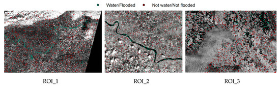
Figure 1.
Study sites in Northern Italy with volunteered geographic information (VGI) assumed as the ground truth points (blue: water and red: non-water) used for (i) learning ordered weight averaging (OWA) aggregation and (ii) validation of the algorithm. ROI: region of interest.

Table 1.
Location/extent of the study sites and characteristics/conditions of the surface water areas. ROI: region of interest.
In the three sites, VGI elements were available, obtained by both in situ observations (in ROI_3) and photointerpretation (in both ROI_1 and ROI_2). In situ observations had been created by agronomists by means of a mobile application within the Space4Agri Project (http://space4agri.irea.cnr.it/it/progetto/struttura/ambito-in-situ-1). Agronomists tagged agricultural parcels with the observed crop, stage of growth and tillage practice. In the case of the rice crop, they indicated if rice paddies were inundated or not (i.e., water or no water) [1]. This VGI was partitioned into two subsets and used as a training set for learning and as a reference set for validation.
Furthermore, other VGIs were created by volunteers through photointerpretation by interacting with a GIS overlaying open street map (OSM) layers, RGB images and other background layers. This VGI consisted of georeferenced observations classified into five classes: “natural flooding”, “flooded fields”, “rivers”, “shadows over water” and “not flooded”. Since assuming VGI as the ground truth is very delicate and risky, as discussed in the huge literature on VGI quality [30,31], we applied a quality assurance and assessment approach [32]. Specifically, for quality assurance, photointerpreters were selected ex-ante and trained to identify the kinds of standing water. Furthermore, since we also reuse VGI created in situ for a different purpose, it was necessary to evaluate its fitness-for-use by applying an ex-post quality assessment approach [32]. Specifically, only in situ VGI elements created close to the dates of acquisition of the multispectral images used for the ESI mapping were selected as reliable VGI. This VGI was assumed as the ground truth and partitioned into three distinct subsets for three distinct objectives: (i) calibrating the definitions of soft constraints, (ii) learning the OWA aggregation and (iii) validation of algorithm performance.
Table 2 reports for each site’s EO satellite data and acquisition dates the number of ground truth pixels (w/nw stand for water/not water) selected from the available reliable VGI used for the soft constraints definition (S) in the preliminary phase, for learning the OWA operator (L) in phase two of the algorithm and for validation (V) of the computed ESI maps. At each validation epoch, 10% (90%) of the ground truth pixels not used for (S) were randomly selected for (L), and the remaining 90% (10%) were used for (V) in the typical (atypical) validation settings, respectively.
Table 2.
Number of pixels (w/nw stand for water/not water) for ROI sites used for the soft constraints definition (S), ordered weight averaging (OWA) learning (L) and 10-fold cross typical/atypical validations (V).
Specifically, the remote sensing data source used in all sites is Sentinel 2 (S2) (https://earth.esa.int/web/sentinel/home). The S2 mission operates as part of a two-satellite system (A and B) providing high-resolution multispectral optical imagery since June 2015 (A) and March 2017 (B). The S2 multispectral instrument (MSI) measures the Earth’s reflected radiance in 13 spectral bands from VIS/NIR to SWIR with a spatial resolution ranging from 10 m to 60 m. The study case was built on S2 data collected for post-event assessments (after flooding occurrences at ROI_1 and ROI_2 and immediately after the rice field survey for ROI_3). Level-2A S2 images were downloaded and preprocessed with a sen2r toolbox [33]. The details of the preprocessing operations are described in [29]. For ROI_1 and ROI_2, Level-2A S2 imagery was downloaded as the bottom of atmosphere (BOA) reflectance through the Copernicus Open Access Hub. Preprocessing consisted of clipping images to our area of interest and masking clouds using the scene classification (SC) product; pixels classified as high and medium cloud probability were masked out, while pixels belonging to different classes were retained to avoid masking-out water pixels. For ROI_3, a BOA image was not available at the desired dates of the field survey in the Copernicus archive, so it was necessary to download the top of atmosphere Level-1C products and apply atmospheric correction by using the Sen2Cor algorithm of the sen2r toolbox library [33].
The processed multispectral products are used to compute the most suitable spectral indexes (SI) reported in Table 3 [18,19,20,21,22,34], which were identified by two experts as indicators enhancing standing water areas presences. They were used as contributing factors from which to derive partial evidence of standing water. The aggregation of partial evidence is performed through an OWA operator [24] generated by applying a machine-learning approach exploiting the limited ground truth obtained by either in situ observations or photointerpretation.
Table 3.
Selected spectral indexes used as contributing factors.
2.2. Theoretical Aspects
In the following subsections, we define the main concepts of fuzzy set theory that are the basic materials and methods used to model the process of environmental status indicator (ESI) mapping.
2.2.1. Soft Constraints
Fuzzy sets were introduced by Zadeh in 1965 [6] to represent concepts characterized by unsharp boundaries, where the transition between membership and non-membership is gradual rather than abrupt. A fuzzy set A on a universe D is characterized by a membership function μA: D → [0, 1], assigning a membership degree, μA(d) ∈ [0, 1], to each element d of the domain D. μA(d) provides an estimation of the belonging of d to A.
An elastic or soft constraint C on a domain D of a variable v (i.e., a contributing factor) is defined by a membership function of a fuzzy subset C of D. When we apply the soft constraint to a value d ∈ D of the variable v, its membership degree μC(d) indicates the degree of satisfaction of C: μC(d) = 1 and means that d fully satisfies C; μC(d) = 0 means that d does not satisfy C at all and 0 < μC(d) < 1 means that d partially satisfies C.
In the case expert’s interpretation of a phenomenon, possibly incomplete and imprecise, a soft constraint can be defined by the domain expert to specify a criterion to compute a partial evidence of the phenomenon given the information on the value of a variable v, which is selected as a contributing factor of the phenomenon. In this case, the expert cannot state precisely which subset of values of the domain D of the contributing factor v provides evidence of the phenomenon but can state imprecise/fuzzy subsets of D.
Soft constraints can be defined with membership functions with different shapes of variable complexity: triangular, trapezoidal, Gaussian-shaped, Bell-shaped, Sigmoid-shaped, etc. A simple definition of a soft constraint μC can be specified with a flexible shape by a tuple (a, b, c, d, e, f), with a, b, c, d ∈ [0, 1] and e, f > 0, as follows:
By setting a = b = − ∞ or c = d = + ∞, we obtain the special cases of L-functions (not increasing) and R-functions (not decreasing) as the ones depicted in Figure 2. By specifying b = c and e = f = 1, we obtain triangular membership functions. By setting e ≠ 1 and f ≠ 1, we can obtain nonlinear functions.
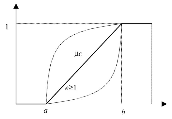
Figure 2.
R-functions defined by (a < b < 1, c = d = + ∞ and e = 1) representing the semantics of a soft constraint.
Complex soft constraints can be defined by combining soft constraints either by conjunction (“C1 and C2” is defined by min(μC1(x), μC2(y)) ∀x ∈ X and ∀y ∈ Y), by disjunction (“C1 or C2” is defined by max(μC1(x), μC2(y)), ∀x ∈ X and ∀y ∈ Y) and by negation (“Not C” is defined by the complement 1 − μC(x)).
Finally, when μC1(x) ⊆ μC2(x), ∀x ∈ X, C1 is included in C2 (i.e., C1 is stricter than C2). When defining a soft constraint to compute the partial evidence degree of a critical phenomenon, stricter soft constraints favor omissions (false negatives) and, conversely, relaxed soft constraints favor commissions (false positives).
2.2.2. Ordered Weighted Averaging (OWA) Operators
The seminal paper [35], stemming from the consideration that “the efficient use of decision support systems (DSSs) is to assist and help humans arrive at a proper decision, but by no means, to replace humans”, proposes to introduce some synergy between human and machine. To this end, the author defines the fuzzy logic-based calculi of linguistically quantified propositions as a viable means for expressing human interpretable decisions.
Linguistic quantifiers were first introduced in [36] as fuzzy subsets of the positive real numbers or of the unit interval [0, 1], according to the fact that they express an absolute quantity, such as many, or a relative quantity, such as most.
Ordered weighted averaging (OWA) operators were first proposed to define an overall decision function aggregating degrees of satisfaction of multiple criteria (in our context, partial evidence degrees computed by soft constraints defined on the domain of some variables) [24]. OWA operators allow us to define fusion strategies with distinct mean-like semantics ranging from the minimum to the maximum of the values they aggregate.
An OWA of dimension N and weighting vector W, with ∑i = 1,...N wi = 1, aggregates N values [d1, …, dN] and computes an aggregated value a in [0, 1], as follows [24,37]:
such that
in which gi is the ith largest value of the d1, dN.
OWA: [0, 1]N→ [0, 1]
a = OWA([d1, ..., dN]) = ∑i = 1, ..., Nwi·gi
A fundamental aspect of the OWA is the reordering of its arguments so that the weight wi is not associated with an argument di but rather with a particular rank of the arguments in decreasing order. A known property of the OWA operators is that they include the max, min and arithmetic mean operators for the appropriate selection of the weighting vector W:
For W = [1, 0, ...., 0], OWA([d1, ..., dN) = max([d1, …, dN]).
For W = [0, ...., 0, 1], OWA([d1, ..., dN]) = min([d1, …, dN]).
For W = [1/N, ...., 1/N], OWA([d1, ..., dN]) = .
It can be proved that OWA operators satisfy the commutativity, monotonicity and idempotency and are bounded by min and max operators [38]:
Min ([d1, ..., dN]) ≤ OWA([d1, ..., dN]) ≤ Max([d1, ..., dN]).
2.3. Proposed Approach
A preliminary phase of the proposed approach is the selection of contributing factors that can influence the phenomenon; these contributing factors are physical variables whose values are computed in all spatial units of a ROI to create thematic maps. They are identified by experts based on domain knowledge; the most suitable shapes of the soft constraint membership functions are selected, exploiting a statistic analysis of the values of the contributing factors on a classified data set. This is done by defining the membership functions that better discriminate the class of interest from the others. Soft constraints satisfaction degrees are interpreted as degrees of partial evidence of the phenomenon due to a specific contributing factor. In this phase, for each factor, an importance degree can be computed proportional to the degree of separability between the classes. This can be determined by applying the soft constraints on the classified data set. Alternatively, for each factor, a degree of reliability or trust can be deemed, depending on the knowledge of the phenomenon or reliability of the data source.
This preliminary step does not need to be performed each time the algorithm is applied to map the ESI on a new ROI. It is done once and for all used classified data from one or more ROIs. Then the automatic algorithm adapts the ESI mapping to a new ROI by exploiting local ground truth.
The automatic algorithm depicted in Figure 3 is structured into two phases. The first phase is mainly knowledge-driven, while the second phase is data-driven.
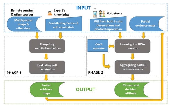
Figure 3.
Workflow of the proposed soft computing adaptive approach for computing environmental status indicator (ESI) maps from remote sensing multispectral images, thematic information and VGI. While phase 1 exploits the expert’s knowledge, phase 2 is data-driven, exploiting VGI. The two phases are decoupled and communicate via the input layer.
In the first phase, after computing the contributing factors on the input map, the input soft constraints are evaluated. This phase produces partial evidence (PE) maps, in which each unit element, a pixel in the illustrated implementation, is associated with a degree in [0, 1].
The second phase exploits reliable VGI in a ROI to learn the best operator, namely, an ordered weighted averaging (OWA) operator [24], for aggregating the PE maps in order to compute the ESI map synthesizing the phenomenon. The choice of OWA operators to model the fusion strategy is due to their mean-like nature, which is recognized by many authors as particularly useful in the context of spatial decision-making [25,39,40,41,42,43,44]. Furthermore, the semantics of the learned aggregation can be expressed linguistically to describe a decision attitude, either optimistic or pessimistic and monarchical or democratic, with blends of these extremes. This aspect confers human understandability to our approach.
Finally, the approach is scalable and suited for a distributing processing implementation framework.
2.3.1. Characterizing the OWA Semantics
To characterize the decision attitude modeled by an OWA operator with weighting vector W, two measures have been introduced in [24]: ORness and dispersion.
The ORness(W) ∈ [0, 1] measure is defined as follows:
This measure characterizes the degree to which the aggregation is like an OR (max) operator. It can be shown that, when the argument values d1, ..., dN are degrees of partial evidence of an anomaly of an environmental phenomenon from N distinct sources (i.e., the greater they are, the more severe the anomaly), we have the following interpretations [39,45]:
ORness[1 , …, 0] = 1 indicates a pessimistic attitude advertising risks (i.e., nothing is disregarded and any single source alone is trusted and taken into consideration to plan preparedness and mitigation interventions so as to minimize the occurrence of risky events);
ORness[0, …, 1] = 0 indicates an optimistic attitude towards tolerating risks (i.e., prioritizing preparedness and mitigation interventions only to anomaly situations pointed out by all sources) and
ORness[1/N, …, 1/N] = 0.5 indicates a balanced and neutral attitude towards risk-prone and risk-adverse.
Another measure used to qualify the semantics of an OWA operator is the dispersion. This measure represents how much of the information in all the arguments is used by an OWA with weighting vector W. The idea behind its definition is that, the greater the dispersion, the more democratic is the aggregation of the correspondent OWA, since it uses information from more sources [46]. Several dispersion measures have been proposed, the first of which is based on the concept of entropy of W. We adopted the dispersion(W) ∈ [0, 1] measure of an OWA operator, as proposed in [46]:
We see that dispersion(W) is clearly symmetric, and, when N is large, it is defined in [0, 1]. When dispersion(W) = 0, it means that only one source is considered; in this case, the aggregation is named monarchical, since the decision is taken just by one. The larger its value, the more the result is determined by additional sources, and, thus, we have a more democratic aggregation.
To linguistically explicit the semantics modeled by an OWA operator with weighting vector W, first one computes its ORness(W) and dispersion(W), as defined in Formulas (3) and (4), respectively. Then, by mapping the point (ORness(W), dispersion(W)) in the 2D space defined by ORness and dispersion shown in Table 4, one can easily select the label representing the decision attitude modeled by the OWA operator. Notice that Table 4 has been defined by considering that high/small arguments of the OWA are pessimistic/optimistic interpretations of the occurrence of a phenomenon that is regarded as undesired, critical, negative or that should not happen. For example, high/small evidence degrees of flood/wildfires/droughts occurrences have a negative/positive flavor. One is then pessimistic/optimistic if the evidence is high/small. Thus, the interpretation of optimism and pessimism reported in Table 4 are complemented with respect to the context of multicriteria decision-making in which generally high/small values are regarded as optimistic/pessimistic evaluations.
Table 4.
Decision attitude as a function of ORness (Φ and dispersion (Δ) in the case of aggregation of N = 8 partial evidence degrees of critical/anomalous event/phenomenon.
When ORness(W) > 0.5 and dispersion(W) is close to 0, the decision is risk-adverse, since one mostly trusts the most pessimistic/towards pessimistic sources and almost disregards the optimistic ones. Nevertheless, in doing this, one may obtain many false positives.
When ORness(W) < 0.5 and dispersion(W) is close to 0, the decision attitude is risk-prone, since one mostly trusts the few sources that are optimistic. In this case, one may miss potential alerting sources and may thus generate many false negatives.
A balanced decision attitude, characterized by ORness(W) = 0.5 and dispersion(W) = (N − 1)/N, takes into account equally all sources, then is both neutral and democratic. Intermediate values of ORness and dispersion characterize different blends of both pessimism/optimism and democracy/monarchy.
2.3.2. Learning OWA Semantics from Observations
One important issue in the domain of partial-evidence aggregation is the determination of the OWA operator modeling the aggregation. If ground truth data are available (e.g., georeferenced observations on the occurrence of a phenomenon at certain locations of the ROI), they can be used to learn the weighting vector of the OWA operator.
To this end we propose the application of a machine-learning approach [47], exploiting VGI assumed as ground truth to learn the best OWA operator for a given ROI by iteratively minimizing error between OWA results at epoch t with respect to the observations described by VGI. Notice that VGI used to this purpose must be quality assessed.
Given K georeferenced observations a1, …, aK assumed as ground truth, for example, VGI elements, by knowing their geographic coordinates, we can associate with each observation the partial evidence values [ai1, …, aiN] having the same coordinates, such that we obtain the following antecedent-consequent rules that must be satisfied:
a11, ...., aN1 → a1
a1K, ...., aNK → aK
a1K, ...., aNK → aK
In principle, the observations a1, …, aK can be specified on a continuous scale [0, 1] to quantify the extent of the phenomenon in the specific location; nevertheless, in practical situations, a discrete scale such as {0, 0.5, 1}, or even a binary scale {0, 1}, is used where 0 means absence of the phenomenon and 1 is presence.
The learning mechanism starts at epoch L = 0 by assuming as initial OWA0 operator the weighted average (balanced and neutral attitude), which is defined with weighting vector W0 = [1/N, …, 1/N]. Then, at each epoch L, it iteratively determines the weighting vector WL = [w1L, …, wNL] of OWAL that minimizes the error existing between the results of its application to all the antecedents of the rules in (5) and the georeferenced observations (i.e., the consequents of the rules).
Formally, this is equivalent to applying the following rule:
where
in which β ∈ (0, 1] is a learning rate parameter and the ith weighting vector element at epoch L is defined as follows:
Λi(L + 1) = Λi(L) − βwiL(argmaxi(a1k, ...., aNk) − OWAL(a1k, ...., aNk)) ∗ (OWAL(a1k, ...., aNk) − ak)
wi L = eΛi(L)/∑j = 1, …, N eΛj(L) ∀i = 1, …, N
2.3.3. Scalability of the Approach
The ESI computation described in the previous section can be implemented in a distributed processing framework represented by the schema depicted in Figure 4.
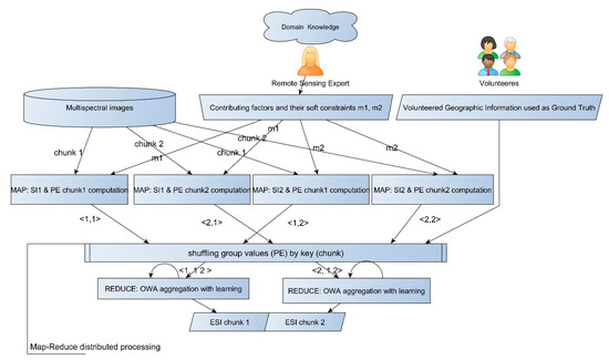
Figure 4.
Map-reduce distributed process computation of the ESI map.
Since the ESI computation is performed independently for each spatial unit and is organized in two subsequent phases, we can implement it in a single round of a map-reduce framework [38].
The map-reduce framework is inspired by the “map” and “reduce” functions used in functional programming. Computational processing occurs on data stored in a distributed file system or within a database, which takes a set of input key-values pairs and produces a set of output key-values pairs [48].
A mapper M is a Turing machine M (<k, v>) → (<k1′, v1′>, …, <ks′, vs′>), which accepts as input a single key-value pair <k, v> and produces a list of key-value pairs <k1′, v1′>, …, <ks’, vs’>.
A shuffle is performed on the outputs of the mappers so as to group the values with the same key: <k1′, v1′, …, vr1′>, …., <kR′, v1′, …, vrR′>.
A reducer R is a Turing machine R: <k′, v1′, …, vr′> → <k′, v″>, which accepts as input a pair <k′, v1′, …, vr′> and produces as output the same key k′ and a new value v″.
A mapper can be instructed by its input parameters to compute more contributing factors and to evaluate more soft constraints on the same chunk; the input key k identifies either a single pixel or a spatial unit in a multispectral image chunk. The associated value v is the information associated with the input chunk (e.g., the bands and theme values such as VGI), plus parameters (the contributing factors’ names and definitions the mapper has to compute) and the tuples (a, b, c, d, e, f) defining the soft constraints membership functions according to definition (1).
A mapper can compute for each pixel in the input chunk the key-value pairs <k1′, v1′>, …, <ks′, vs′>, where ki′ identifies the chunk and vi′ are the computed degrees of partial evidence of the SIs in the chunk.
Successively, the reducers execute the second phase by aggregating the partial evidence maps v1′, …, vr1′ of the same chunk ki′ in parallel so as to compute the ESI map v″ for the chunk.
Chunks are finally recombined by mosaicing at the end of the process.
The values v″ are computed by applying in each pixel or spatial unit of the chunk the OWA operator learned by leveraging VGI in the ROI covered by the chunk. This way, each reducer can learn a distinct OWA operator; thus, adapting the ESI computation to the local context and observations. Notice that the learning process is performed within each reducer module, which applies on its input chunk the OWA operator learned at time epoch L based on the subset of VGI included in the input chunk. There is no need to upload the input at each epoch, since the evidence maps do not change from epoch to epoch; once the optimal OWA has been determined, the ESI map can be computed and stored on disk.
2.3.4. Contributions from Expert’s Knowledge
In order to exploit the huge literature based on single spectral index (SI) for mapping water surfaces and vegetation cover, seven SIs have been selected as contributing factors from which partial evidence of standing water can be computed (see Table 3). Besides SIs, also hue (H) and value (V) dimensions of the HSV color space, derived by transforming the components SWIR2, NIR and RED, were selected to define the reduced space hue-value (HV) as a further contributing factor; in this transformed space, standing water surfaces can be separated from land surfaces by means of empirical thresholds, as defined in [22].
The transformation function f: SWIR2 × NIR × RED → H × V is a standardized colorimetric transformation from RGB to HV components of the HSV color space, where SWIR2 = R, NIR = G and RED = B respectively, defined as in [49]:
For each contributing factor/spectral index, a soft constraint is defined on its domain by the expert by analyzing the statistical distribution of each SI value for the pixels corresponding to standing water with respect to the ones of nonwater surfaces, according to a classified data set. The soft constraints are defined with a shape, basically L and R functions, as defined in Formula (1). In the case of the contributing factor HV, a single bi-dimensional soft constraint on the domain H × V has been defined as a fuzzy relation combining by minimum the soft constraints on the two dimensions. The details of this activity preliminary to the execution of the algorithm phase 1 are reported in [29].
In order to set up a validation experiment aimed at testing the stability of the approach when changing experts, we performed phase 1 twice by exploiting interpretations provided by two experts, hereafter named A and B, respectively. They defined different soft constraints on the same set of contributing factors by interpreting available classified data, as illustrated in Figure 5. The used classified data were VGI created by photointerpretation. The two experts have distinct decision attitudes: A, who defined piece-wise linear membership functions, was generally more optimistic than B, who also defined nonlinear functions in order to better discriminate “not flooded” areas. In fact, it can be noticed that the soft constraints of expert A are generally stricter than those defined by expert B on the same SI (i.e., the membership functions defined by expert A are generally included in those of expert B). It follows that expert A (Figure 5) has a more optimistic attitude towards mapping standing water areas (considered as an undesired phenomenon); he/she accepts the risk of generating omission errors by partially disregarding “shadows over water areas”. Conversely, expert B (Figure 5) takes a more pessimistic attitude by defining soft constraints so as not to miss “shadows over water areas”, which belong to the support of the membership functions (i.e., have not null membership degree).
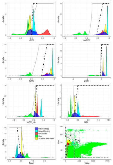
Figure 5.
Black dotted lines identify soft constraints defined by expert A with a risky attitude (i.e., optimistic) in mapping standing water, regarded as a negative phenomenon, by taking into account the ability of soft constraints to separate the distributions of standing water (comprising the three classes: “natural flooding”, “flooded fields” and “rivers”) with respect to the “not flooded” class. The grey continuous lines identify the soft constraints defined by expert B with a precautionary attitude (i.e., pessimistic) by taking into account the ability of soft constraints to separate the distributions of standing water (comprising the four classes: “natural flooding”, “flooded fields”, “rivers” and “shadows over water”) with respect to the “not flooded” class. Notice that the bottom–right diagram illustrates the two pairs of soft constraints on the hue and value of the triad HSV defined by experts A and B.
2.4. Validation Experiments
The validation experiment was designed with the following objectives:
- (a)
- to compare the accuracy of the proposal with respect to traditional approaches based on a single SI,
- (b)
- to investigate the stability of results with respect to changing the ROI,
- (c)
- to investigate the stability of results with respect to changing experts (A and B),
- (d)
- to investigate the adaptability of the learning to local context (ROI) by changing experts (A and B) and
- (e)
- to investigate the accuracy when downscaling the dimension of the training set.
In phase 1 of the algorithm partial evidence (PE), maps are computed for each contributing factor using as input the preprocessed multispectral images, the definitions of contributing factors and soft constraints defined by either expert A or B. The PE maps are successively used by phase 2 to the aim of learning the OWA operator and then computing the overall ESI map.
Phase 1 was executed twice: the first execution by using the soft constraints by expert A and the second by expert B, respectively. Thus, we obtained two distinct sets of PE maps, indicated hereafter by PE_A and PE_B.
Figure 6 shows an example of PE_A maps derived by four different contributing factors on the three ROIs. It can be seen that soft constraints on H and V contributing factors generate maps (l), (m) and (n), characterized by high contrast in all ROIs. Pixel values are mostly distributed close to the extreme of the domain [0, 1]; this indicates that the classification of standing water by using the soft constraints on H and V components is less affected by doubts. This happens also for the other contributing factors in ROI_1 (Emilia area). Conversely, in ROI_2 and ROI_3, the soft constraints defined on AWEI (b, c); mNDWI (e, f) and NDFI (h, i) yield more gradual PE_A maps, thus, bearing more uncertainty.
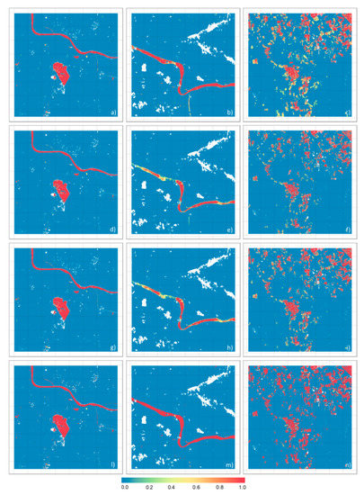
Figure 6.
Partial-evidence maps obtained by soft constraints of expert A on AWEI (a–c); mNDWI (d–f); NDFI (g–i) and the hue (H) and value (V) components (l–n) for zoom areas of 20 km × 20 km of ROI_1 Emilia area (left), ROI _2 Po Valley (middle) and ROI _3 rice paddies (right). Cloud-masked areas are white, and the degree of partial evidence ranges in [0, 1] [29].
Phase 2 of the algorithm takes as input one set of PE maps generated by a run of phase 1, either PE_A or PE_B, and a subset of VGI and computes an ESI map. This consists in aggregating PE maps by applying the OWA operator learned by the iterative process exploiting VGI. Outputs of this phase are: the ESI map, the weighting vector of the OWA operator, its ORness and dispersion measures and the correspondent label (as defined in Table 4) representing the decision attitude modeled by the OWA operator.
By changing either PE maps or VGI, different ESI maps can be computed for the same ROI; specifically, phase 2 was executed several times with distinct VGI subsets, as described in the following subsection.
The algorithm phase 1 was executed twice on the three ROIs to the aim of testing stability and adaptability to ROI when changing experts (objectives c and d).
Accuracy of each single contributing factor in mapping standing water was evaluated by computing accuracy metrics true positives (TP), true negatives (TN), false positives (FP) and false negatives (FN) from the confusion matrix, commission (CE = FP/(FP + TP)) and omission (OE = FN/(FN + TP)) errors and F-score defined as follows:
Figure 7 reports the diagram of variation of the F-score measure in the three ROIs (shown in Figure 1) obtained by using single contributing factors. Ground truth for the validation is composed of around 1000 VGI independent elements in each ROI, as reported in the fourth column of Table 2. Values of F-scores were computed by defining increasing thresholds on the SI domains, normalized in [0, 1] with a 0.1 step; pixels with SI values exceeding the threshold are considered as “standing water”. It can be noticed that F-score curves are not increasing. This is because, by increasing the threshold, we are stricter on the selection of standing water pixels; thus, while commission errors remain stable, we may increase omission errors by missing true standing water areas.
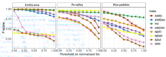
Figure 7.
Diagrams show the variation of the F-score in the three ROIs for eight distinct SIs defined in the literature for mapping standing water areas; pixels considered as “watered” have SI values above a threshold varying in [0, 1].
It can be observed that in the three ROIs which are characterized by distinct land covers and water conditions (water depth, color, fractional cover, plant/soil patches presence, etc.), a different SI presents the best performance (greatest F-score) for given values of the thresholds. This confirms our intuition that a single SI cannot capture all types of standing water conditions.
In the Emilia area, HV, AWEI and NDFI have the best comparable performance for all thresholds; in the Po Valley area, the best index is NDWI, followed by HV. Finally, in the rice paddies area, AWEI and HV are the best indices for threshold values below and above 0.3, respectively.
These results confirm the need of an aggregation phase capable of automatically selecting the best-performing contributing factor for each pixel in each ROI.
This is achieved in phase 2, which applies an adaptation of the algorithm to a specific ROI by exploiting available ground truth.
In order to pursue the validation with a traditional setting of the training set and with a downscaled training set, we designed two kinds of k-fold cross-validation experiments.
We recall that a k-fold cross validation is a statistical method aimed at evaluating the performance of a learning algorithm by changing the training set; in doing so, it is possible to compute both average performance metrics and the standard deviation to assess its sensitivity.
In each experiment, using either expert A or B, phase 2 was executed 10 times (k = 10), thus generating ten weighting vectors of the OWA and, consequently, 10 distinct ESI maps for the site. At each run, a different subset of both ground truth data for learning and testing were selected by applying stratified random sampling. In the first kind of validation experiments, we first used 90% of ground truth VGI elements for learning the OWA aggregation and 10% for testing, as in the standard validation methods of machine-learning. These experiments are named typical (T) k-fold cross validations.
To test the algorithm with a downscaled training set, we performed two other 10-fold cross validations by using A and B but a different proportion of the learning and testing sets. Differently than in the typical validations, this time we used a small subset of VGI elements for learning (only 10% of the available ground truth pixels), while we used the remaining 90% for testing. Stratified random sampling was applied to select the two subsets. This validation is called atypical (AT) and was aimed at investigating the stability of the results when simulating a realistic situation with a small set of ground truth data.
Performance achieved on each ROI by the typical and atypical 10-fold cross validations is shown in Figure 8; the ten F-score diagrams in each area are relative to the ten ESI maps produced as a result of the ten executions of the algorithm phase 2 using either A or B. Table 5 summarizes average performances of the algorithm over all runs and all thresholds in both the typical and the atypical validations when using A and B and when using the single-best SI in each ROI. Table 6 reports the learned OWA operator, averaged over the 10 runs when using both A and B in both the typical (T) and atypical (AT) validation settings.
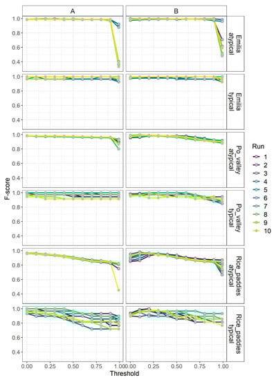
Figure 8.
F-score diagrams on the three ROIs in the typical and atypical 10-fold cross validations using soft constraints defined by experts A and B. Parameters used for k-fold cross validations: k = 10, learning rate = 0.5 and number of epochs = 500.
Table 5.
Average, standard deviation and average minimum F-score values over all 10 runs of the algorithm and all thresholds in the typical (T) and atypical (AT) validations using soft constraints defined by expert A and B and based on the best-performing SI on the ROI. Best results are highlighted in bold.
Table 6.
Learned weighting vectors of the OWA operator in each ROI averaged over the 10 runs of both the typical (T) and atypical (AT) 10-fold cross validation for experts A and B. The table also reports the values of the approximated weighting vector, the average ORness (Θ), the ORness standard deviation (STD(Θ)), the dispersion (Δ) and correspondent decision attitude.
Finally, Figure 10 illustrates for each ROI two ESI maps highlighting in blue “standing water” areas identified by values of ESI > 0.5 computed based on either A or B.
In the following, we discuss the results reported in the figures and tables.
3. Results and Discussion
The ESI computed by the proposed approach has the following main characteristics.
An ESI value is defined in [0, 1] and can be computed at the spatial unit level (i.e., either a pixel or a larger spatial unit). In the study case, the ESI value was computed for each individual pixel, since we did not have polygons delimiting spatial units of interest.
The ESI map can be tuned to local context and observation conditions. In the study case, we considered three ROIs with distinct environmental conditions presenting peculiar “standing water” characteristics and provenance of VGI, either created in situ or by photointerpretation.
The proposed algorithm can model distinct decision-maker needs by modeling distinct attitudes towards risks. Specifically, when defining a soft constraint to compute the partial evidence degree of a critical phenomenon, the stricter the soft constraint, the more we may miss the phenomenon; i.e., we have a risky attitude and tolerate false negatives. Conversely, by defining a relaxed soft constraint, we have a precautionary attitude but may set false alarms of the phenomenon; i.e., we tolerate false positives. Furthermore, the aggregation performed by OWA operators [39] can model blends of decision attitudes in between the two extremes: optimistic–pessimistic and monarchical–democratic.
ESI computation is feasible in a distributed processing framework on big (geo)data in order to achieve scalability. It is well-known that map-reduce was designed for processing massive data sets and that its bottleneck is the number of rounds needed to implement an algorithm. Programs require that every reducer only has access to a portion of the input, and the strict modularization prohibits reducers from communicating within a round. These conditions are satisfied by our proposed algorithm; it does not need both multiple rounds for implementing the ESI computation and any communication to occur among mappers and among reducers during a round. Simply, distinct mappers can be instructed to execute the first phase for generating distinct partial evidence maps by processing in parallel the given image chunks based on the expert’s knowledge provided in input as both contributing factors and soft constraints definitions.
Learning the aggregation operator can make results less sensible to expert interpretations. In fact, when defining distinct contributing factors and soft constraints, the first phase computes different PE maps; thus, the process learns the best OWA operator given the current evidence maps for each ROI in which VGI is available.
These findings are discussed below.
3.1. Comparison with Traditional Approaches
Table 5 shows that our proposal achieves results equal or better than those yielded by the best single SI in all the three ROIs. Although performances are only slightly better in the Po Valley and Emilia area, an advantage of our proposal is that it can select automatically the best SIs for each single pixel in each site to determine the ESI value. This operation is not possible when using current approaches of multicriteria aggregation based on weighted average, in which the weight is always associated with the same criterion for all pixels in an ROI. By contrast, our algorithm is adaptive to the local conditions and can recognize the distinct aspect of standing water.
One important observation can be made by comparing the average F-scores of the proposed approach in the three ROIs: the worst results are those in the rice paddies site in both the typical and atypical validations. This is probably due to the different kind of VGI used for learning and validation, mainly created in situ by a field operator, with respect to the VGI used in the other two sites, created by photointerpreters.
Specifically, the VGI elements created in situ were selected with a date closely preceding the date of acquisition of the used multispectral image, since an acquisition date during the survey period was unavailable. Thus, the status of “standing water” in a rice paddy could be slightly different when observed in situ by the agronomist and when observed remotely by the satellite sensor. Moreover, it is important to remind that this ROI is the most complex to classify due to the heterogeneity of inundated rice fields characterized by a mixture of water, soil and plants. Finally, the agronomic flooding induced by human management is an abrupt process that can change from field to field, while hazard flooding generally covers distributed areas with similar topography and water persists on the ground for some days.
3.2. Stability of the Results by Changing ROI
Figure 8 shows that in all ROIs and in the typical validation setting, F-score diagrams are quite stable and maintain high values for all thresholds using both experts.
In the atypical setting, the F-scores for some of the 10 runs decrease for high thresholds (above 0.9), especially in the Emilia and rice paddies ROIs. This may depend on the small dimensions of the learning set used, which for some runs may not represent well all types of surface water. Nevertheless, as seen in Table 5, in all ROIs, average F-scores are high in both the typical and atypical validations; in the Emilia and Po Valley, average F-scores are above 0.95, while in the rice paddies site, are above 0.90.
3.3. Stability of the Results by Changing Expert
From Table 5, we can notice that expert B gets slightly better results than expert A in the Emilia and rice paddies sites, while A performs better in the Po Valley site. This is confirmed in both the typical and atypical validations. A reason of this result can depend on the different nature of “standing water”. In the Emilia and rice paddies sites, flooded areas and inundated rice fields are present covering a mixture of situations (different water depth and patches of soil and vegetation). In such conditions, a precautionary attitude is more appropriate to map different kinds of standing water, while the risky attitude of expert A generates more false negatives. In the Po Valley site, where we have a river water without influence of signal due to substrate or vegetation but only of water optical properties, a more optimistic (i.e., risky) attitude is the best choice, since it does not generate so many false positives, having just one kind of standing water in a continuous and homogeneous patch (i.e., constrained river bed). Furthermore, the stability of the results in terms of the standard deviation are also better for B in both typical and atypical validations and in all the three ROIs. In Figure 8, the atypical validation with expert A has a more consistent decreasing trend of some diagrams with respect to B. This again can be interpreted as due to the more optimistic attitude towards mapping an undesired phenomenon (i.e., risky attitude) of expert A; by considering as “standing water” only pixels with an ESI > 0.9, more omission errors are produced by A with respect to B, who applied a more precautionary attitude.
3.4. Adaptability to Local Context and Experts Contributions
Table 6 reports for each site the average OWA operator learned in both the typical and atypical validations for experts A and B. Specifically, it shows the weighting vector averaged over the runs of the 10-fold cross validation, the average ORness of the learned OWAs, the correspondent standard deviation, the dispersion measure and the decision attitude (selected based on ORness and dispersion values, as listed in Table 4). It can be noticed that the algorithm can adapt to the ROI characteristics by learning a distinct OWA vector that is also stable (i.e., low standard deviation in each ROI). Finally, the decision attitudes of the learned OWA operators do not change in the typical and atypical validation settings for a given expert and ROI.
In the Emilia area with expert A, the algorithm yields an OWA characterized by an average ORness of 0.8 and a correspondent dispersion of 0.6 in both the typical and atypical validations, respectively. This corresponds to the attitude “semi-democratic and toward pessimism”. Specifically, the aggregation mostly uses the greatest five (four) arguments to compute the ESI value in the typical (atypical) settings, although with a different weight. Thus, the ESI value increases depending on, at most, the greatest five (four) partial evidence degrees, and there is not a unique contributing factor that alone determines the ESI map.
In the other two ROIs, the ORness is 1 and the dispersion is 0, which corresponds to a “monarchical and pessimistic” attitude, in which the greatest partial evidence degree is the only determining ESI values. This means that in each pixel, ESI is determined by a single contributing factor; yet, due to the nature of the OWA, the contributing factor can be different from pixel to pixel, thus allowing to capture the distinct aspects of standing water.
On the other side, with expert B, the algorithm adaptation mechanism learns different OWA aggregations in each ROI. As shown in Figure 9, the learned OWAs are stable in two out of the three ROIs. In the Po Valley and rice paddies sites, the generated OWA corresponds to the “semi-monarchical and toward pessimism” decision attitude, while, for expert A, it was “monarchical and pessimistic”. This means that a more synergic aggregation is needed to optimize the ESI computation with B than with A.
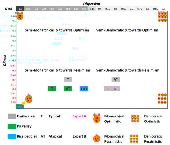
Figure 9.
ORness–dispersion space in which the OWA operators learned in each ROI (identified by rectangles with distinct colors: grey in the Emilia area, green in the Po Valley and light-blue in the rice paddies) in the typical (T) and atypical (AT) validations for experts A (in violet) and B (in black) are positioned according to their ORness and dispersion measures.
In the Emilia ROI, the typical and atypical validations yield two OWA operators, which differ for the dispersion and not for the ORness. Although close to one another, they correspond to different decision attitudes: “semi-monarchical and toward pessimism” in the typical validation and “semi-democratic and towards pessimism” in the atypical one. Both these aggregations compute positive ESI values only in presence of at least two (three) positive partial-evidence degrees.
Generally, in all ROIs with expert B, the learned aggregations have smaller ORness than with A (i.e., OWAB is more optimistic than OWAA).
We also have aggregations with greater dispersion (i.e., OWAB more democratic than OWAA), with the exception of the typical validation in the Emilia area.
These findings explicit the roles of the adaptation mechanism depending on the expert. In the case of expert A, in the Po Valley and rice paddies ROIs, the learned aggregation fully “trusts” the most pessimistic partial evidence. This allows to counterbalance the optimistic and risky attitude of expert A, who defined strict soft constraints by disregarding “shadows over water”. Too many omission errors could be generated by applying a synergic aggregation, which instead is appropriate in the Emilia area.
In the case of expert B, more partial-evidence degrees are aggregated in a synergic way to compute ESI values so as not to obtain too many commission errors, which may cause false alarms. In this way, the adaptation mechanism tries to contrast the precautionary attitude of expert B.
Figure 10 shows for each ROI two ESI maps generated with experts A and B. It can be seen that the standing water areas are quite similar in each pair of maps of the same ROI. This is exactly what we expected; the algorithm, although using different experts and a different VGI, is robust and stable, producing very similar ESI maps on each ROI.
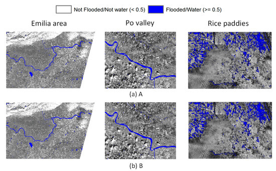
Figure 10.
ESI maps in the three ROIs obtained by using interpretations of the two experts A and B and by averaging the weighting vectors of the OWA operators learned on 10 runs of the algorithm in the atypical settings. Values considered as standing water are in blue and are obtained by a threshold on ESI > 0.5.
3.5. Performance of Typical and Atypical Validations
This objective is aimed at assessing if our algorithm can produce acceptable results in a realistic situation in which the available ground truth is scarce, below 100 VGI elements. Of course, large training sets provide a better chance of understanding underlying patterns, rather than just learning to identify specific examples. Nevertheless, learning from specific examples available in a local context can be effective if we assume that a local context is characterized by the presence of a specific kind of standing water and if we use the results just for that area.
In Figure 8, we can observe that independently of the expert and up to a threshold of 0.9, the F-score values are very high in both the typical and atypical validations. For thresholds above 0.9, the F-score has a greater decreasing rate for the atypical validation compared to the typical one. This means that when we have a small ground truth set for the adaptation to the ROI, one must be careful when segmenting the resulting ESI map to identify the standing water areas. We have to choose a threshold that is below 0.9 to avoid generating too-high omission error rates. On the other side, when considering a threshold on ESI > 0, we can be confident on the high accuracy of the ESI mapping obtained, even when performing a learning based on a small ground truth set.
4. Conclusions
The proposed approach for ESI mapping applies both soft computing and machine-learning, two branches of artificial intelligence. It is a transparent approach; it represents and manages the semantics of expert’s interpretations, possibly vague, by means of soft constraints on contributing factors. Furthermore, it learns an aggregation strategy of the interpretations whose semantics can be expressed linguistically, thus, pursuing human understandability. Moreover, the aggregation can model distinct needs by inheriting the properties of OWA operators [39]: the distinct credit of the contributing factors and reliability of their sources and the possibility to model distinct attitudes towards risks in between the two extremes of optimistic and pessimistic, monarchical and democratic. The learning mechanism exploits the properties of OWA operators to adapt the ESI mapping to the local context by copying with the subjectivity of experts. Finally, a remarkable aspect of the algorithm is that it does not require a huge amount of VGI to achieve high accuracy.
In this respect, one important aspect is assuring and assessing the quality of VGI used as ground truth, since low quality or inappropriate VGI can lead to poor results. As discussed in Section 3.5, using the ground truth to train the algorithm by VGI created in situ for a different purpose leads to a lower results accuracy, with respect to using VGI by photointerpretation.
In the future, stricter quality assessment criteria should be used to select VGI elements.
Future work is needed to confirm these findings. Primarily, a more extensive validation on other sites had to be done to assess robustness depending on different contexts. Second, the approach should be tested by exploiting both different contributing factors and a reduced number of them. We intend on exploring the use of all single spectral bands as contributing factors and directly defining the soft constraints on their domains. This could be regarded as defining fuzzy spectral signatures of “standing water”. Furthermore, scientific literature on standing water mapping based on single SIs would be worth considering as an alternative “expert”. The thresholds on the single SIs could be used to define “crisp” constraints to compute binary degrees of partial evidences of “standing water”. Finally, the approach should be applied for different purposes, such as to detect burned areas, ice and snow area on glaciers, evidence of droughts sites and crop damage/stress in agriculture.
Author Contributions
Conceptualization, G.B.; methodology, G.B., M.B., P.A.B., and D.S.; software and validation, A.G.; data curation, A.G., D.S., and M.B.; writing and editing, G.B.; review, all authors and funding acquisition, G.B. All authors have read and agreed to the published version of the manuscript.
Funding
This work has been conducted within the frame of the Fondazione CARIPLO Project “STRESS: Strategies, Tools and new data for Resilient Smart Societies” #2016-0766; “Bando Fondazione Rst—Ricerca dedicata al dissesto idrogeologico, 2016” and SIMULATOR-ADS Project #137287, co-funded by the Regione Lombardia & FESR “Linea R&S per Aggregazioni”.
Acknowledgments
We want to thank the anonymous reviewers whose valuable work greatly helped us to improve our manuscript.
Conflicts of Interest
The authors declare no conflicts of interest.
References
- Bordogna, G.; Frigerio, L.; Kliment, T.; Brivio, P.A.; Hossard, L.; Manfron, G.; Sterlacchini, S. “Contextualized VGI” Creation and Management to Cope with Uncertainty and Imprecision. ISPRS Int. J. Geo Inf. 2016, 5, 234. [Google Scholar] [CrossRef]
- Humanitarian Open Street Map. Available online: https://www.hotosm.org/docs/ (accessed on 10 October 2019).
- Arcaini, P.; Bordogna, G. Geotemporal Querying of Social Networks and Summarization. In Encyclopedia of Social Network Analysis and Mining, 2nd ed.; Alhajj, R., Rokne, J., Eds.; Springer: Berlin/Heidelberg, Germany, 2018. [Google Scholar]
- Sivarajah, U.; Kamal, M.M.; Irani, Z.; Weerakkody, V. Critical analysis of Big Data challenges and analytical methods. J. Bus. Res. 2017, 70, 263–286. [Google Scholar] [CrossRef]
- Bordogna, G.; Pagani, M.; Pasi, G. A Flexible Decision support approach to model ill-defined knowledge in GIS. In Geographic Uncertainty in Environmental Security; Morris, A., Kokham, S., Eds.; Springer: Berlin/Heidelberg, Germany, 2006. [Google Scholar]
- Zadeh, L.A. Fuzzy Sets. Inf. Control 1965, 8, 338–353. [Google Scholar] [CrossRef]
- Lecun, Y.; Bengio, Y.; Hinton, G.E. Deep Learning. Nature 2015, 521, 436–444. [Google Scholar] [CrossRef] [PubMed]
- Reichstein, M.; Camps-Valls, G.; Stevens, B. Deep learning and process understanding for data-driven Earth system science. Nature 2019, 566, 195–204. [Google Scholar] [CrossRef] [PubMed]
- Zhang, L.; Zhang, L.; Du, B. Deep Learning for Remote Sensing Data: A Technical Tutorial on the State of the Art. IEEE Geosci. Remote Sens. Mag. 2016, 4, 22–40. [Google Scholar] [CrossRef]
- Castelluccio, M.; Poggi, G.; Sansone, C.; Verdoliva, L. Land Use Classification in Remote Sensing Images by Convolutional Neural Networks. arXiv 2015, arXiv:1508.00092. [Google Scholar]
- Larochelle, H.; Bengio, Y.; Louradour, J.; Lamblin, P. Exploring strategies for training deep neural networks. J. Mach. Learn. Res. 2009, 10, 1–40. [Google Scholar]
- Han, X.; Zhong, Y.; Cao, L.; Zhang, L. Pre-Trained AlexNet Architecture with Pyramid Pooling and Supervision for High Spatial Resolution Remote Sensing Image Scene Classification. Remote Sens. 2017, 9, 848. [Google Scholar] [CrossRef]
- Acharya, T.D.; Subedi, A.; Lee, D.H. Evaluation of water indices for surface water extraction in a Landsat 8 scene of Nepal. Sensors 2018, 18, 2580. [Google Scholar] [CrossRef]
- Ji, L.; Zhang, L.; Wylie, B. Analysis of Dynamic Thresholds for the Normalized Difference Water Index. Photogramm. Eng. Remote Sens. 2009, 11, 1307–1317. [Google Scholar] [CrossRef]
- Estoque, R.C.; Murayama, Y. Classification and change detection of built-up lands from Landsat-7 ETM+ and Landsat-8 OLI/TIRS imageries: A comparative assessment of various spectral indices. Ecol. Indic. 2015, 56, 205–217. [Google Scholar] [CrossRef]
- Dempewolf, J.; Trigg, S.; DeFries, R.S.; Eby, S. Burned-Area Mapping of the Serengeti—Mara Region Using MODIS Reflectance Data. IEEE Geosci. Remote Sens. Lett. 2007, 4, 312–316. [Google Scholar] [CrossRef]
- Qiu, B.; Zhang, K.; Tang, Z.; Chen, C.; Wang, Z. Developing soil indices based on brightness, darkness, and greenness to improve land surface mapping accuracy. GISci. Remote Sens. 2017, 54, 759–777. [Google Scholar] [CrossRef]
- Boschetti, M.; Nutini, F.; Manfron, G.; Brivio, P.A.; Nelson, A. Comparative analysis of normalised difference spectral indices derived from MODIS for detecting surface water in flooded rice cropping systems. PLoS ONE 2014, 9. [Google Scholar] [CrossRef] [PubMed]
- Feyisa, G.L.; Meilby, H.; Fensholt, R.; Proud, S.R. Remote sensing of environment automated water extraction index: A new technique for surface water mapping using Landsat imagery. Remote Sens. Environ. 2014, 140, 23–35. [Google Scholar] [CrossRef]
- Huete, A.R. A soil-adjusted vegetation index (SAVI). Remote Sens. Environ. 1988, 25, 295–309. [Google Scholar] [CrossRef]
- McFeeters, S.K. The use of the normalized difference water index (NDWI) in the delineation of open water features. Int. J. Remote Sens. 1996, 17, 1425–1432. [Google Scholar] [CrossRef]
- Pekel, J.F.; Vancutsem, C.; Bastin, L.; Clerici, M.; Vanbogaert, E.; Bartholomé, E.; Defourny, P. A near real-time water surface detection method based on HSV transformation of MODIS multi-Spectral time series data. Remote Sens. Environ. 2014, 140, 704–716. [Google Scholar] [CrossRef]
- Xu, H. Modification of normalised difference water index (NDWI) to enhance open water features in remotely sensed imagery. Int. J. Remote Sens. 2006, 27, 3025–3033. [Google Scholar] [CrossRef]
- Yager, R.R. On ordered weighted averaging aggregation operators in multi-criteria decision making. IEEE Trans. Syst. Man Cybern. 1988, 18, 183–190. [Google Scholar] [CrossRef]
- Malczewski, J. GIS-based multicriteria decision analysis: A survey of the literature. Int. J. Geogr. Inf. Sci. 2006, 20, 703–726. [Google Scholar] [CrossRef]
- Brivio, P.A.; Boschetti, M.; Carrara, P.; Stroppiana, D.; Bordogna, G. Fuzzy integration of satellite data for detecting environmental anomalies across Africa. In Advances in Remote Sensing and Geoinformation Processing for Land Degradation Assessment; Hill, J., Roeder, A., Eds.; Taylor & Francis: London, UK, 2006. [Google Scholar]
- Carrara, P.; Bordogna, G.; Boschetti, M.; Brivio, P.A.; Nelson, A.D.; Stroppiana, D. A flexible multi-source spatial-data fusion system for environmental status assessment at continental scale. Int. J. Geogr. Inf. Sci. 2008, 22, 781–799. [Google Scholar] [CrossRef]
- Bordogna, G.; Boschetti, M.; Brivio, P.A.; Carrara, P.; Pagani, M.; Stroppiana, D. Fusion Strategies based on the OWA Operator in Environmental Applications. In Recent Developments in the Ordered Weighted Averaging Operators: Theory and Practice, 1st ed.; Kacprzyk, J., Yager, R.R., Beliakov, G., Eds.; Springer: Berlin/Heidelberg, Germany, 2011. [Google Scholar]
- Goffi, A.; Stroppiana, D.; Brivio, P.A.; Bordogna, G.; Boschetti, M. Towards an automated approach to map flooded areas from Sentinel-2 MSI data and soft integration of water spectral features. Int. J. Appl. Earth Obs. Geoinf. 2020, 84, 101951. [Google Scholar] [CrossRef]
- Senaratne, H.; Mobasheri, A.; Ali, A.L.; Capineri, C.; Haklay, M. A review of volunteered geographic information quality assessment methods. Int. J. Geogr. Inf. Sci. 2017, 31, 139–167. [Google Scholar] [CrossRef]
- Bordogna, G.; Carrara, P.; Criscuolo, L.; Pepe, M.; Rampini, A. On predicting and improving the quality of Volunteer Geographic Information projects. Int. J. Digit. Earth 2016, 9, 134–155. [Google Scholar] [CrossRef]
- Bordogna, G.; Carrara, P.; Criscuolo, L.; Pepe, M.; Rampini, A. A linguistic decision making approach to assess the quality of volunteer geographic information for citizen science. Inf. Sci. 2014, 258, 312–327. [Google Scholar] [CrossRef]
- Ranghetti, L.; Busetto, L. Sen2r: An R Toolbox to Find, Download and Preprocess Sentinel-2 Data, R Package Version 1.0.0; Available online: http://sen2r.ranghetti.info (accessed on 10 October 2019).
- Shen, L.; Li, C. Water body extraction from landsat ETM + imagery using adaboost algorithm. In Proceedings of the 2010 18th International Conference on Geoinformatics, Beijing, China, 18–20 June 2010. [Google Scholar]
- Kacprzyk, J. Fuzzy Logic with Linguistic Quantifiers: A Tool for Better Modeling of Human Evidence Aggregation Processes? Adv. Psychol. 1988, 56, 233–263. [Google Scholar]
- Zadeh, L.A. A computational approach to fuzzy quantifiers in natural languages. Comps. Math. Appl. 1983, 9, 149–184. [Google Scholar] [CrossRef]
- Yager, R.R. Quantifier guided aggregation using OWA operators. Int. J. Intell. Syst. 1996, 11, 49–73. [Google Scholar] [CrossRef]
- Dean, J.; Ghemawat, S. Mapreduce: Simplified data processing on large clusters. Commun. ACM 2008, 51, 107–113. [Google Scholar] [CrossRef]
- Yager, R.R. New modes of OWA information fusion. Int. J. Intell. Syst. 1998, 13, 661–681. [Google Scholar] [CrossRef]
- Bloch, I.; Maître, H. Information combination operators for data fusion: A comparative review with classification. IEEE Trans. Syst. Man Cybern. 1996, 26, 52–67. [Google Scholar] [CrossRef]
- Bone, C.; Dragicevic, S.; Roberts, A. Integrating high resolution remote sensing, GIS and fuzzy set theory for identifying susceptibility areas of forest insect infestations. Int. J. Remote Sens. 2005, 26, 4809–4828. [Google Scholar] [CrossRef]
- Chanussot, J.; Mauris, G.; Lambert, P. Fuzzy fusion techniques for linear features detection in multitemporal SAR images. IEEE Trans. Geosci. Remote Sens. 1999, 37, 1292–1305. [Google Scholar] [CrossRef]
- Jiang, H.; Eastman, J.R. Application of fuzzy measures in multi-criteria evaluation in GIS. Int. J. Geogr. Inf. Sci. 2000, 14, 173–184. [Google Scholar] [CrossRef]
- Robinson, P.B. A perspective on the fundamentals of fuzzy sets and their use in Geographic Information Systems. Trans. GIS 2003, 7, 3–30. [Google Scholar] [CrossRef]
- Bordogna, G.; Pagani, M.; Pasi, G. Imperfect Multisource Spatial Data Fusion Based on a Local Consensual Dynamics. In Uncertainty Approaches for Spatial Data Modeling and Processing; Kacprzyk, J., Petry, F.E., Yazici, A., Eds.; Springer: Berlin/Heidelberg, Germany, 2010. [Google Scholar]
- Yager, R.R. On the dispersion measure of OWA operators. Inf. Sci. 2009, 179, 3908–3919. [Google Scholar] [CrossRef]
- Filev, D.P.; Yager, R.R. On the issue of obtaining OWA operator weights. Fuzzy Sets Syst. 1998, 94, 157–169. [Google Scholar] [CrossRef]
- Karloff, H.; Suri, S.; Vassilvitskii, S. A model of computation for MapReduce. In Proceedings of the Twenty-First Annual ACM-SIAM Symposium on Discrete Algorithms, Austin, TX, USA, 17–19 January 2010. [Google Scholar]
- Smith, A.R. Color Gamut Transform Pairs. In Proceedings of the 5th Annual Conference on Computer Graphics and Interactive Techniques, New York, NY, USA, 23–25 August 1978; Volume 12, pp. 12–19. [Google Scholar]
© 2020 by the authors. Licensee MDPI, Basel, Switzerland. This article is an open access article distributed under the terms and conditions of the Creative Commons Attribution (CC BY) license (http://creativecommons.org/licenses/by/4.0/).