Validation of the SNTHERM Model Applied for Snow Depth, Grain Size, and Brightness Temperature Simulation at Meteorological Stations in China

Abstract

Validation of the snow process model is an important preliminary work for the snow parameter estimation. The snow grain growth is a continuous and accumulative process, which cannot be evaluated without comparing with the observations in snow season scale. In order to understand the snow properties in the Asian Water Tower region (including Xinjiang province and the Tibetan Plateau) and enhance the use of modeling tools, an extended snow experiment at the foot of the Altay Mountain was designed to validate and improve the coupled physical Snow Thermal Model (SNTHERM) and the Microwave Emission Model of Layered Snowpacks (MEMLS). By matching simultaneously the observed snow depth, geometric grain size, and observed brightness temperature (T_B), with an RMSE of 1.91 cm, 0.47 mm, and 4.43 K (at 36.5 GHz, vertical polarization), respectively, we finalized the important model coefficients, which are the grain growth coefficient and the grain size to exponential correlation length conversion coefficients. When extended to 102 meteorological stations in the 2008–2009 winter, the SNTHERM predicted the daily snow depth with an accuracy of 2–4 cm RMSE, and the coupled SNTHERM-MEMLS model predicted the satellite-observed T_B with an accuracy of 13.34 K RMSE at 36.5 GHz, vertical polarization, with the fractional snow cover considered.

1. Introduction

The seasonal snow cover, as an important component of the cryosphere, plays a key role in the climate system [1,2]. The high albedo of the snow surface, the latent heat generated by the internal ice/water phase transition, and the adiabatic effect of the snow layer significantly shift the energy balance and influence the energy exchange between the atmosphere, the snow cover, and the underlying soil medium. The snow is a natural reservoir of solid water resources. The snow-redistributed energy drives the circulation and redistribution of water. As a result of these reasons, the snow is an important parameter in the climate numerical model and the hydrological model predictions [3]. However, the snow feedback mechanisms on the climate change in long-term scale remains uncertain [4], which requires improvements in the snow-related property simulation.

An accurate simulation of snow parameters (including the snow depth, temperature, density, grain size, albedo, etc.) and the water and energy fluxes (including radiation fluxes, evaporation, sublimation, melting rates, etc.) are the key to understand the function of the snow cover on the weather, climate, and hydrological cycles. The lack of snow water equivalent (SWE) within the global circulation models breaks the water balance and changes energy balance, and leads to uncertainties in the climate predictions [5,6,7,8,9]. When the meteorological forcing data is accurate, a good snow process model can predict all the parameters listed above. However, when applied for a vast region where the meteorological forcing data is biased or of coarse resolution and the remote sensing technique is affected by the clouds or other nuisance parameters, a data assimilation (DA) framework is needed to take the advantages of both methods. The validation of the snow process model can provide an error estimation for the DA system. The coupling of the snow process model and the radiative transfer model is the key to assimilate the satellite observations.

There are many land surface mass and energy balance models that have included the evolution of snowpack processes [10], such as the Biosphere–Atmosphere Transfer Scheme (BATS) [11], Community Land Model (CLM) [12], Hydrology Tiled ECMWF Scheme of Surface Exchanges over Land model (HTESSEL) [13], Interactions between Surface, Biosphere, and Atmosphere model (ISBA) [14,15], Joint UK Land Environment Simulator model (JULES) [16], Met Office Surface Exchange Scheme (MOSES) [17], ORganising Carbon and Hydrology In Dynamic EcosystEm (ORCHIDEE) [18], and Canadian Land Surface Scheme (CLASS) [19]. There are many differences between these models, which are firstly expressed in the number of snow layers simulated, secondly shown in the parameterizations of each piece of the snow-related physical or chemical process, and thirdly reflected in the discretization of time and space and the partial differential equation (PDE) numerical resolution. Some snow models have included more complete snow evolution mechanism and unconfined number of snow layers to simulate fine-resolution snow stratigraphy, such as the Crocus [20], SNOWPACK [21], and Snow Thermal Model (SNTHERM) [22]. Many studies have demonstrated that the snow stratigraphy, i.e., layered properties of snow micro-structure (snow grain size), snow density, snow temperature, and snow wetness, is important for the radiative transfer model to match the observed passive microwave observations [23,24,25,26]. When the Simplified Simple Biosphere 3.0 (SSiB3) land surface model coupled the SNTHERM grain growth mechanism but the original three snow layer framework was kept, Li et al. (2015) [27] found the snow micro-structure parameter of the bottom snow layer had to be tuned after a large snowfall instead of using the mass-weighted average value, because the model resampled and merged the middle and bottom snow layers of different grain sizes from the previous time step, but averaged out the microwave signal sensitivity. Therefore, the use of a snow process model considering more snow layers is important.

Among the snow parameters, the snow grain size and snow depth are important for the data assimilation utilizing passive microwave observations. The snow particles produce volume scattering at high frequencies [28]. For dry snow, an increased snow depth or snow micro-structure dimension strongly can decrease the brightness temperature at 37 GHz high frequency, and this feature is the fundamental basis for passive microwave SWE retrieval [29]. The snow density changes the interface reflectivity between the air-snow-soil boundaries and snow interfaces and shows some extent of influence on modeled T_B. However, the magnitude of T_B response to density from 100 to 400 kg/m³ varies from less than 10 K to about 40 K according to different snow emission model simulations [30]. In this case, the influence of snow density can hardly be considered strong and clear. The snow T_B equals the product of snow emissivity and snow temperature. However, the influence of temperature is much smaller compared to grain size and snow depth (see Table IV of [31]). For wet snow, the existence of liquid water can dramatically increase the T_B by changing the dominant snow emission mechanism from volume scattering to absorption [26]. In High Mountain Asia, Kwon et al. (2019) [32] presented that wet snow showed a different SWE versus ΔT_{B, 18V-36V} relationship with the dry snow and degraded the DA performance. In this paper, the measured liquid water content was not available for validation. Therefore, our validation for T_B was constrained in the dry snow time period. After excluding the wet snow influence, the grain size is possible to be validated using the observed brightness temperature if the estimated snow depth is correct.

The validation of the multi-layer snow process model [1,21] and the further coupling with the microwave radiative transfer model [33,34,35] had been conducted previously for deep snow in Weissflühjoch, Switzerland, Sodankylä, Finland, Colorado, USA. However, the measurement of layered snow parameters (especially snow micro-structure parameter) for an entire snow season of several months is still laborious. In recent years, only a few validation dataset is available, like the Nordic Snow Radar Experiment (NoSREx) in Finland [36]. For snow model validation in China, a new in-situ snow experiment is better to be deployed, because the snow in the world varies in type, depth and properties driven by the diverse local meteorological conditions [37]. In the previous studies, Lehning [21] validated his newly-established CROCUS model using the grains size measurements at Weissfluhjoch during the 1997–1998 and 1998–1999 winters, but without modeled T_B validated. Brucker et al. (2011) [1], Huang et al. (2012) [33], Sandells et al. (2017) [34], and Kang et al. (2019) [35] compared the simulated snow depth, micro-structure parameter (geometric grain size, D_max, optical grain size, D_o, or exponential correlation length, p_ex) and T_B with the observations together. However, sometimes, when the simulated micro-structure parameter does no match the observations due to the snow process model error or the differences in parameter definition (see [38] for more details) between the simulations and the observations, the snow process model simulation was not corrected before inputting to the radiative transfer model [34,35], whereas the later may also has its own parameter definition and requirement (like stickiness, τ, and the bi-continuous model statistical parameters, $‹\xi ›$ and b). In the end, it will result in a complex, uncertain and highly empirical conversion coefficient, which is sensitive to both the choice of the snow process model and the choice of radiative transfer model. This situation is not propitious to expanding the DA algorithm globally, since each model combination needs to be validated for all regions.

In this paper, we aimed to validate the SNTHERM model and the coupling of SNTHERM with the Microwave Emission Model of Layered Snowpacks (MEMLS) based on Improved Born Approximation [39,40] for a vast region in the western part of China, including Xinjiang, Qinghai, and Xizang (Tibet) provinces. Multiple studies have demonstrated that SNTHERM is capable of simulating the snow properties accurately at diverse locations and under different conditions [10,34,41,42]. The validation in our paper was conducted at meteorological sites situated at flat areas. The snow depth there in most cases is less than half a meter, which is much less compared to the previous studies [1,41,42]. At the Altay National Reference Meteorological station at the foot of the Altay Mountain, we designed and implemented a five-month snow experiment to measure the snow and soil properties and corresponding brightness temperature (T_B) for the model validation. Because both the simulated and the observed snow micro-structure parameter is the geometric grain size, after excluding the temperature dependency (accurately estimated as a prerequisite condition), the grain growth coefficient of SNTHERM is able to be updated with some extent of confidence. Afterwards, we validated the geometric grain size (D_max) to exponential correlation length (p_ex) conversion coefficient for the SNTHERM-MEMLS coupling, which had been validated previously for snow at Sodankyla, Finland, Colorado, US, and Churchill, Canada [43]. In the end, the same snow process and radiative transfer models and coefficients were extended to simulate the snow depth and brightness temperature at 102 meteorological stations in three provinces, in the 2008–2009 winter. In this validation for a large area, we utilized the satellite observed brightness temperature from Advanced Microwave Scanning Radiometer for Earth Observing System (EOS) (AMSR-E), with the influence of not fully-covered snow considered using the fractional snow cover area (FSC) retrieved from Moderate-resolution Imaging Spectroradiometer (MODIS) reflectance. This paper will be organized as follows: in Section 2, the implementation of the Altay experiment in the 2017–2018 winter and the meteorological station datasets in the Xinjiang, Qinghai, and Tibet study area in the 2008–2009 winter are introduced. In Section 3, the SNTEHRM model and the model improvement theories, equations, and parameters are represented. The MEMLS model is also briefly introduced. Section 4 shows the results of the improved SNTHERM performance, the validation of snow and soil parameters, and the validation of brightness temperature for the Altay experiment and the 102 stations. The last two sections are the Discussions and the Conclusions.

2. The Altay Experiment, Study Area, and the Datasets Utilized

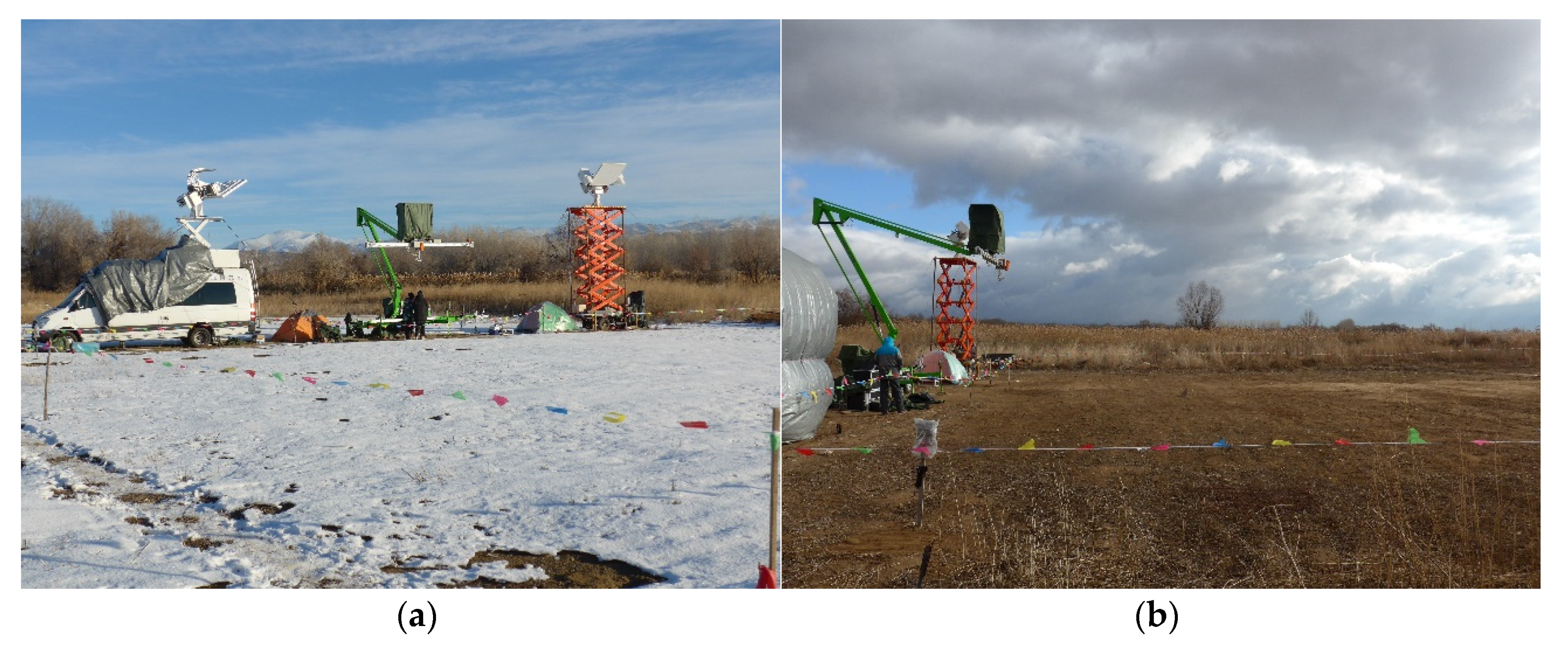
2.1. The Altay Experiment

The Altay Experiment from October 26th, 2017 to March 10th, 2018 at the Altay National Reference Meteorological station (47°44′26.58″N, 88°4′21.55″) was designed and implemented by the State Key Laboratory of Remote Sensing Science, affiliated to the Institute of Remote Sensing and Digital Earth (RADI), Aerospace Information Research Institute (AIR) of the Chinese Academy of Sciences (CAS), and supported by the Northwest Institute of Eco-Environment and Resources (NIEER) of the Chinese Academy of Sciences (CAS).

We reached the site on October 22th, 2017, and installed the L, C, and X band radiometer from the Institute of Remote Sensing and Digital Earth (RADI) and the L, Ku, and Ka band radiometer from the Northwest Institute of Eco-Environment and Resources (NIEER). The observed field has a dimension of 50 m in the North-South direction and 30 m in the East-West direction. As can be seen from Figure 1, the grass was mowed carefully before the first snowfall to prepare a bare soil background for the microwave modeling. On the north edge of the observed field, from west to east, the RADI radiometer, a ground-based synthetic aperture radar system (SAR) and the NIEER radiometer were installed in sequence. The radiometers provided the brightness temperature measurements at 1.4, 6.925, 10.65, 18.7, and 36.5 GHz at 2 to 3 h steps. Manufactured by the RPG-XCH-DP (Radiometer Physics GMbH) company, the radiometers installed a stable noise diode that support an automatic gain calibration to keep their stability for several months. This noise injection module, together with the temperature stable reference at the other side of the Dicke switch, provides two calibration points to correct the system noise equivalent temperature (T_n) and the system gain (G). The non-linearity of the system can be assumed unchanged for its intrinsic stability. Both the RADI and the NIEER radiometers were sky-tipping calibrated when they were first installed. Later, the manually controlled sky tipping calibrations were implemented for the RADI radiometer on clear-sky conditions approximately per month. The NIEER radiometer was not further sky tipping calibrated, because it is found due to the sensitivity of 36.5 GHz to water vapor content, the sky tipping calibration introduced more errors and was no better than the automatic calibration.

On November 10th, 2017, the first snowfall covered the observed field. Starting from this day to March 11th, 2018, a total of 109 snowpits were excavated within 50 m distance to the radiometers. For each snowpit, different snow layers were recognized by observing the color and crystal size of the snow and feeling the snow hardness by fingers. For each snow layer, the thickness, geometric grain size, and temperature were measured. The thickness was measured by a woolen folding ruler. The geometric grain size was measured by post-processing photos of a large amount of snow particles on a 2 mm × 2 mm crystal card taken by a high-resolution Leica camera. The snow density was measured by a 250 mL wedge-type sampler (10 cm × 10 cm × 5 cm) at per 5 cm step. Before the first snowfall, three Decagon 5TM soil sensors were buried at −2, −5, and −10 cm depth below the soil surface to provide the soil temperature and the equivalent volumetric water content (unfrozen part) by measuring the dielectric constant of the soil. The data was collected by an Em−50 series logger.

Figure 2 shows an example of the snowpit observed on 15:34 January 24th, 2018. The snow had 4 layers with a thickness of 4.5 cm, 2 cm, 2.5 cm, and 7.5 cm from top to bottom. Figure 2b–e shows the corresponding snow particle photos for each layer. The geometric snow grain size was post-processed using the method as follows. First, a human-computer interactive program was coded to georegistrate the photo using the 2-mm grid intersections. Then, an interactive dialog box was called to save the two ends of the maximum dimension (diameter) of one particle visually recognized and clicked by the observer. Only two observers were involved in the snow particle digitization, and the final result was checked and corrected by a single one. The X, Y coordinates of the paired points were converted to the lengths by the computer. Each photo was separated into 16 subphotos, and in each subphoto at least 10 particles were digitalized. Using the over 160 particles, the geometric grain size (D_max) was calculated using the mean of the maximum dimensions, according to the definition in Mätzler (2002) [38].

From the Altay meteorological station, we acquired the hourly air temperature, precipitation, wind speed, relative humidity, air pressure, and solar radiation to drive SNTHERM. The hourly soil temperature was also provided. We utilized the measured soil temperature at −320 cm depth as the low boundary condition, whereas the upper boundary condition is the air temperature. The required downwelling longwave radiation forcing data was from the 3-h 0.25 degree resolution Noah model Global Land Data Assimilation System (GLDAS) dataset [44]; its influence will be discussed by comparing the SNTHERM simulated and the station measured net radiation in Section 5.2.

2.2. The Study Area and the Datasets Utilized

The study area is the Xinjiang, Qinghai, and Xizang (Chinese name, English name is: Tibet) provinces in China, which can be considered as the extended Asian Water Tower (AWT) region. These three provinces are far from the ocean and have a dry weather. The solar radiation is stronger on the high-elevation Tibetan Plateau (TP), which is not beneficial to retain the snow cover. In the flat area, snow cover in the northern part of Xinjiang can last for over 5 months, whereas most new snow disappeared within 2 weeks on the TP unless the snowfall is heavy enough or the site is shaded, north-faced, or on high mountains. The snow disappearance is attributed from the strong sublimation, melting of the topmost snow layer under strong solar radiation (although the air temperature is below 0 °C), and from the wind blowing effect. The night on the TP is cold in the winter months, and it can refreeze the snow surface to maintain a dry snow condition at AMSR-E descending overpass time (1:30 a.m. local time approximately).

The accuracy of the snow parameter estimation is determined by the accuracy of the models themselves and the forcing data. From the National Meteorological Information Center of the China Meteorological Administration (CMA), we got the daily meteorological datasets to support our research. Figure 3 is a map of three provinces marked by the locations of the reference meteorological sites. The entire meteorological dataset given to us has 134 sites, whereas we used only 102 sites. At some sites, there was no snowfall in the 2008–2009 winter (magenta pentagon), average snow depth below 1 cm (red triangles), or incomplete data to support SNTHERM running (blue stars); these sites were not used. Most of the sites not used locate around the Taklimakan Desert in the southern Xinjiang or in the Qaidam Basin in the northern Qinghai.

The daily dataset from the meteorological stations was merged with the 3-h 0.25 degree resolution Noah model Global Land Data Assimilation System (GLDAS) dataset [44]. The SNTHERM 3-h meteorological forcing is produced as follows. For the air temperature, the measured daily mean, maximum and minimum measurements were provided by the stations. On each day, the GLDAS per 3 h simulations were translated to the daily statistics. Using the three points (mean, maximum, and minimum), a simple linear model, as T_measured = a + b × T_GLDAS, was used to generate the corrected GLDAS air temperature, with a and b fitted. For the relative humidity and wind speed, the GLDAS values were corrected by comparing with the daily mean measurements, using a scaling model as Y_measured = a × Y_GLDAS (Y represents the parameter). For the precipitation, the same scaling model is utilized to match the observed per 12 h total precipitation (8:00–20:00 and 20:00–8:00). SNTHERM requires only one average air pressure, and thus we utilized the average daily mean air pressure measured from November 2008 to March 2009.

The only tuned parameter is the radiation flux. Only 13 sites have the daily mean solar radiation measurements. Four of them locate in Tibet, 4 in Qinghai, and 5 in Xinjiang provinces. For these sites, the measured daily solar radiation was merged with GLDAS using the scaling model. The statistics showed the GLDAS daily solar radiation has a 20% relative error at most. Therefore, for the other sites, it is allowed to tune the time-series downwelling shortwave and longwave radiation on all days by a same factor between 0.8 to 1.2. There is no further artificially tuning for certain specific days.

The satellite AMSR-E T_B observations used for validation are from the reprocessed MEaSUREs Calibrated Enhanced-Resolution Passive Microwave Daily EASE-Grid 2.0 Brightness Temperature (EnTB) [45]. The nominal spatial resolution is 3.125 km at 36.5 and 89 GHz, 6.25 km at 18.7 and 23.8 GHz, and 12.5 km at 6.925 and 10.65 GHz. We utilized the highest resolution at each frequency for the model comparison.

3. Models

3.1. Snow Thermal Model (SNTHERM) Introduction

The SNTHERM (Snow THERmal Model) [22] was published by Rachel Jordan working in the Cold Regions Research & Engineering Laboratory (CRREL) in 1989. It is a one-dimensional model, which aimed to accurately predict snow temperature and snowmelt using the meteorological forcing data of air temperature, relative humidity, air pressure, wind speed, precipitation, and radiation fluxes. The model can calculate the snow albedo using the simulated snow grain size and the upwelling longwave radiation using the simulated snow temperature. We activated these modules, and therefore only the downwelling shortwave and longwave radiations are needed.

In SNTHERM, the snow-covered land surface is modeled as several layers of snow and soil medium, with the vegetation neglected. Its mass balance includes the precipitation (snow, rain, sleet), sublimation, and evaporation at the snow surface and the liquid water and water vapor movement in the snow layers. Its energy balance includes the radiation balance, turbulent fluxes (sensible + latent heat), and convective heat from precipitation at the snow surface, soil heat flux at the bottom of the snow, and the heat conducted and carried by mass fluxes in the snow layers. Most snow process models, complex or simple, considered the same flux terms. A the diagrammatic explanation of the SNTHERM physical processes was published on the CRREL website (https://www.erdc.usace.army.mil/Media/Fact-Sheets/Fact-Sheet-Article-View/Article/476650/sntherm/) and can be referred for a better understanding of these fluxes.

Within the snowpack, the SNTHERM considers the snow temperature and phase change, snow compaction and the snow grain growth. The grain growth module is unique, dependent on snow temperature, but simpler than the SNOWPACK and Crocus models, as:

$$\frac{\partial d}{\partial t}=\frac{g_1\left|U_v\right|}{d}=\frac{g_1}{d}{D}_{c0s}\left(\frac{1000}{P_a}\right){\left(\frac{T}{273.15}\right)}^6{C}_{KT}\left|\frac{\partial T}{\partial z}\right|$$

(1)

where d is the SNTHERM-simulated grain size [m], t is the time [s]. This equation calculates the change of d per second. U_v is the water vapor pressure [kg·m⁻²·s⁻¹]. D_c0s is the effective diffusion coefficient for water vapor at 1000 hPa and 0 °C [m²/s]. P_a is the air pressure [hPa]. T is the snow temperature [K]. C_KT is the derivative of the equilibrium water vapor density with respect to temperature [kg·m⁻³·K⁻¹]. $\partial T/\partial z$ is the snow temperature gradient [K/m]. The g₁ is an adjustable variable, hereafter we called it the grain growth coefficient. g₁ was first determined by matching the observed ‘grain diameter’. According to the magnitude of the grain size measurements (written as ‘0.04–0.2 mm for new snow, 0.2–0.6 mm for fine-grained older snow and 2.0–3.0 mm for older snow near 0 °C’) and the time of the study (in 1960s to 1980s), the definition of the SNTHERM d is closer to the geometric grain size (D_max). In [22], it suggested a default value of g₁ as 5.0 × 10⁻⁷ m⁴/kg. Due to the semi-empirical natural of g₁, in this paper, it is considered as a revisable parameter and is planned to be updated according to the Altay snowpit measurements.

3.2. Snow Thermal Model (SNTHERM) Improvement

The published SNTHERM code from the CRREL website was composed in 1989 and updated in 2002. Starting from 2010, we did a series of revisions. Some revisions are related to bug fixing. For example, one line was added as follows: after the snow density is calculated by snow mass divided by layer thickness, an instant check of the calculated density is carried out—if the snow density is larger than 917 kg/m³, reduce it to 917 kg/m³ and correct the layer thickness to keep snow mass unchanged. A maximum snow layer thickness limit of 5 cm was added to prevent an abrupt melting rate when a very thick layer suddenly reaches 0 °C. The use of SNTHERM module to calculate snow albedo instead of a user-defined constant value was set as a mandatory option. More important, the SNTHERM89 code has a module to consider the influence of soil background on the shallow snow albedo, written in the shallow.f function. It is of critical importance for simulations in our study region and was activated.

In the original SNTHERM code, although the snowmelt flux is calculated at the bottom-most snow layer, such flux was not inputted to the topmost soil layer. The soil moisture can only be changed due to water vapor movement, which is of tiny magnitude compared to the liquid water movement. The SNTHERM can be run starting from an initial snowpack status. However, to reduce the reliance on the in-situ measurements, our choice is to start SNTHERM from before the snow season. The rainfall and the snow melted water can change the soil water mass. The later further influences the thermal properties of the soil layer, and consequently influences the snow temperature via the soil heat flux. Therefore, for the sake of physical validity, we thought the simulation of the soil water movement process is needed, and should be implemented for all soil layers for completeness. It can be added to the SNTHERM modeling framework by providing the liquid water mass flux, U_l [kg m⁻² s⁻¹], at the bottom of each soil layer. In this case, the downward drainage of water from the snowpack into the soil layers is allowed.

According to Darcy’s law, U_l can be calculated as [46,47],

$$U_l=-{\rho }_l{k}_l\left(1+\frac{\partial \psi }{\partial z}\right)$$

(2)

where U_l is defined as positive in the upward direction. ρ_l is the liquid water density, 1000 kg/m³. k_l is the hydraulic conductivity [m/s]. ψ is the soil matric potential [m], defined in negative values (otherwise, the sign before $\partial \psi /\partial z$ in Equation (2) should be negative). z the vertical position [m]. $\partial \psi /\partial z$ is unitless.

We utilized the Van-Genuchten (1980) (VG80) soil-water retention curve model [48] to calculate k_l and $\partial \psi /\partial z$. The hydraulic conductivity is a product of saturated hydraulic conductivity (k_s) and relative hydraulic conductivity (k_r) as:

$$k_l=k_s{k}_r=k_s{S}_e^{\frac{1}{2}}{\left[1-{\left(1-S_e{}^{\frac{1}{m}}\right)}^m\right]}^2$$

(3)

where, S_e is the effective liquid water saturation, defined in SNTHERM and also in [48] as:

$$S_e=\frac{\theta -{\theta }_r}{{\theta }_s-{\theta }_r}=\frac{s-s_r}{s_s-s_r}$$

(4)

where, θ is the volumetric soil water content [m³/m³], and θ_s and θ_r are the saturated and the irreducible volumetric soil water content. s is the unitless liquid water saturation, defined as $\theta /\varphi$. $\varphi$ is the soil porosity, calculated as $1-{\rho }_b/{\rho }_s$, where ${\rho }_b$ is the soil bulk density [kg/m³] and ${\rho }_s$ is the soil specific density [kg/m³]. S_e based on θ or s is the same for soil.

m is the VG80 model shape factor, and has a relationship as m = 1 − 1/n with the other shape factor, n. The soil matric potential is related to S_e as [49]:

$$\psi \left(S_e\right)=-\frac{1}{\alpha }{\left[S_e^{-\frac{n}{n-1}}-1\right]}^{\frac{1}{n}}$$

(5)

where α [m⁻¹] is a VG80 model parameter, defined as positive hereafter; it is the inflection point where the slope of $\partial \theta /\partial \psi$ reaches its maximum value. Then,

$$\frac{\partial \psi }{\partial z}=\frac{\partial \psi }{\partial S_e}\frac{\partial S_e}{\partial z}=\frac{1}{\alpha \left(n-1\right)}\frac{{\left[S_e^{-\frac{1}{m}}-1\right]}^{-m}}{S_e^{1+\frac{1}{m}}}\frac{\partial S_e}{\partial z}$$

(6)

Following the SNTHERM modeling framework, $\partial S_e/\partial z$ was discretized to $\left(S_{e,i}-S_{e,i-1}\right)/\left(0.5\times \left(\Delta z_i+\Delta z_{i-1}\right)\right)$, and inputted into a big matrix to solve S_e at each layer. We also added a further adjustment of k_l for frozen soil according to Equation (5) of [50].

U_l calculated from the bottom-most snow layer is used as a boundary condition for the topmost soil layer. If j is the topmost soil layer, its discretized water balance equation at time t is:

$$C{7}^j\left(S_e^{j,t}-S_e^{j,t-\mathsf{\Delta }t}\right)=-0.5{\left\{U_l^{j+1}+{\rho }_l{k}_l^{j-\frac{1}{2}}\left(1+{\left(\frac{\partial \psi }{\partial S_e}\right)}^{j-\frac{1}{2}}\frac{S_e^j-S_e^{j-1}}{0.5\times \left(\Delta z_j+\Delta z_{j-1}\right)}\right)\right\}}^t-0.5{\left\{U_l^{j+1}-U_l^j\right\}}^{t-\mathsf{\Delta }t}+M_j$$

(7)

where $\mathsf{\Delta }t$ is time step, $\mathsf{\Delta }z$ is layer thickness. c7 is the conversion factor from S_e to liquid water mass change rate, and M is the phase change term; see Jordan (1991) [22] (pp. 30) for more details.

Originally, the SNTHERM code has only two default soil type choices: sand and clay, and only the thermal parameters were given. To check the soil model performance, we conducted three groups of calculations, as listed in

Table 1. The soil modeling parameter settings.

Parameters	Scenario 1	Scenario 2	Scenario 3
SNTHERM soil modelling structure	Original SNTHERM89 code	New SNTHERM with soil water movement	New SNTHERM with soil water movement
Soil type	clay soil type	extended clay soil type with hydraulic parameters added	Altay site-specific soil type
Soil texture	Not determined	22% sand, 20% silt, 58% clay	35% sand, 46% silt, 19% clay
Specific density [kg/m3]	2700
Bulk density [kg/m3]	1000		1323
Heat capacity [J·kg−1·K−1]1	800		832.4
Dry soil thermal conductivity [W·m−1·K−1]	0.113		0.156
Thermal conductivity of dry solids [W·m−1·K−1]	3.43		6.06
Plasticity index2	0.23		0.1
Soil albedo	0.4
Soil emissivity	0.9
Irreducible volumetric water content [m3/m3]	Not used	0	0.004
Saturated volumetric water content [m3/m3]	Not used	0.36	0.42
Saturated hydraulic conductivity [cm/min]4	Not used	0.00294	0.0164
α [1/cm] 4	Not used	0.00855	0.348
n	Not used	1.08	1.50
m	Not used	0.07	0.33
Initial soil temperature status	Temperature measurements at −5, −10, −15, −20, −40, −80, −160, and −320 cm depth
Soil temperature boundary condition	Time-varying temperature at −320 cm depth
Initial soil water content status	10% volumetric water content for all layers		10% volumetric water content for layers above −22 cm depth, and 20% for the layers below
Soil water content status boundary condition	Constant bottom layer soil moisture

¹ Heat capacity in J·m⁻³·K⁻¹ was converted to that in J·kg⁻¹·K⁻¹ by dividing the specific density in kg/m³. ² J_p [22] (pp. 20) is used for calculating the soil freezing curve, i.e., the unfrozen liquid water fraction changed with soil temperature. ³ Technical report [22] suggested 0.15; however the SNTHERM89 code actually uses 0.2. ⁴ k_s and α are translated to values in m/s and 1/m during the computation.

. In the 1st scenario, we used the original SNTHERM89 code choosing a clay soil type. In the 2nd scenario, we added the soil water movement for clay soil, and assumed a soil texture of 22% sand, 20% silt, and 58% clay fractions, according to the clay soil setting in the CLM model [51]. Then, the soil hydraulic parameters (θ_s, θ_r, $\alpha$, n, and m) were able to be calculated using the Carsel and Parrish (1988) model listed in [49] (eq. C3). In the 3rd scenario, the soil texture (35% sand, 46% silt, and 19% clay fractions) and porosity (0.51) at the Altay station was extracted from the GLDAS soil dataset (https://ldas.gsfc.nasa.gov/gldas/soils) to calculate the thermal coefficients using [51] and VG80 model parameters using [49]. During the thermal coefficient calculation, an equivalent organic fraction of 0.1033 was reverted from the texture and porosity, using Equation (3) in [51], and used to calculate the dry soil thermal conductivity, thermal conductivity of dry solids, and heat capacity, using Equations (7), (10), and (14) in [51], respectively. Table 1 lists the values of these parameters.

In the 1st scenario when the original SNTHERM code was utilized, it was found a minimum extent of bug fixing (3 lines) is needed to produce a normal, comparable simulation result. We listed these debugging efforts in the Appendix A. To maintain the consistency with scenarios 2 and 3, in scenario 1, we also turned on the snow albedo calculation module and the shallow snow albedo correction module.

In simulation for the Altay experiment, the time-varying soil temperature at −320 cm depth is used as the boundary condition during the temperature calculation. The initial status of soil temperature was set according to the measurements at −5, −10, −15, −20, −40, −80, −160, and −320 cm depth. The Decagon 5TM sensor only measured the soil moisture of the top 10 cm, as about 10% volumetric water content. The volumetric water content in the 1st and 2nd scenarios were set homogenous as 10%. A constant volumetric water content at −320 cm depth was set as the boundary condition for the S_e calculation. We have found setting the volumetric water content below −22 cm depth as 20% gave better temperature simulation for the top soil layer, and therefore this setting was used for the 3rd scenario. The reason is uncertain, but could have compensated for lots of impacting factors, like the inhomogeneous soil hydraulic parameters and time-varying soil moisture boundary condition.

The SNTHERM simulation for the 102 stations started from August 1st 2008 to August 1st 2009. the initial status of soil was set according to GLDAS data on August 1st and a constant soil temperature and moisture boundary condition was utilized. The soil parameters were set the same as the Altay site-specific soil values. An improvement in future can be utilizing the local GLDAS soil parameters or the Wei et al. (2013) [52] dataset suggested in Tables 2 and 3 of [53].

3.3. Brightness Temperature Model

The snow brightness temperature was simulated by the Microwave Emission Model of Layered Snowpacks (MEMLS) (Mätzler and Wiesmann, 1999) [39] based on the Improved Born Approximation (IBA) [40]. It is a multiple layer snow radiative transfer model, which uses the temperature, snow micro-structure parameter (exponential correlation length, p_ex, in its case), density, and thickness of all snow layers and the background soil reflectivity at vertical and horizontal polarizations to calculate the brightness temperature observed from the snow surface. The IBA considers the multiple-scattering of diffuse radiation between the snow particles. In MEMLS, when the snow radiation is emitted out from the air-snow boundary, the trapped radiation due to total internal reflection (TIR) is considered using 6-flux radiative transfer equation resolution. The MEMLS model details are explicitly presented in [39,40], and a further model explanation can also be found in [43].

The soil reflectivity model was the frequency-independent QHNfi model written in [54]. It is a semi-empirical model with the coefficients recently refitted using the field measurements covering a wide range of bare soil conditions and frequencies at 1.4 to 90 GHz.

MEMLS requires an exponential correlation length (p_ex) whereas SNTHERM simulates the geometric grain size (D_max). We utilized the equation and coefficients validated in [43] to do the D_max to p_ex conversion:

$$p_{ex}=0.23+0.13\times log\left(D_{max}\right)$$

(8)

The brightness temperature simulated by MEMLS is for fully-covered snow. In order to represent the AMSR-E brightness temperature in the pixel that nests the meteorological station, a fractional snow cover (FSC) retrieved from the 7-band MODIS reflectance [55,56] is used to calculate the pixel T_B as:

$$T_{B,pixel}=FSC\times T_{B,MEMLS}+\left(1-FSC\right)\times e_{background}\times T_{background}$$

(9)

where e_background is the background emissivity at certain frequency calculated before the first snowfall when air temperature is close to 0 °C. T_background in theory should be the background physical temperature uncovered by snow. It is not the SNTHERM-simulated topmost soil temperature beneath the snowpack because the uncovered soil does not have the thermal insulation from the snow. T_background should have a stronger sensitivity but less fluctuation compared to the air temperature. As a compromise, we utilized the top snow layer temperature.

4. Results

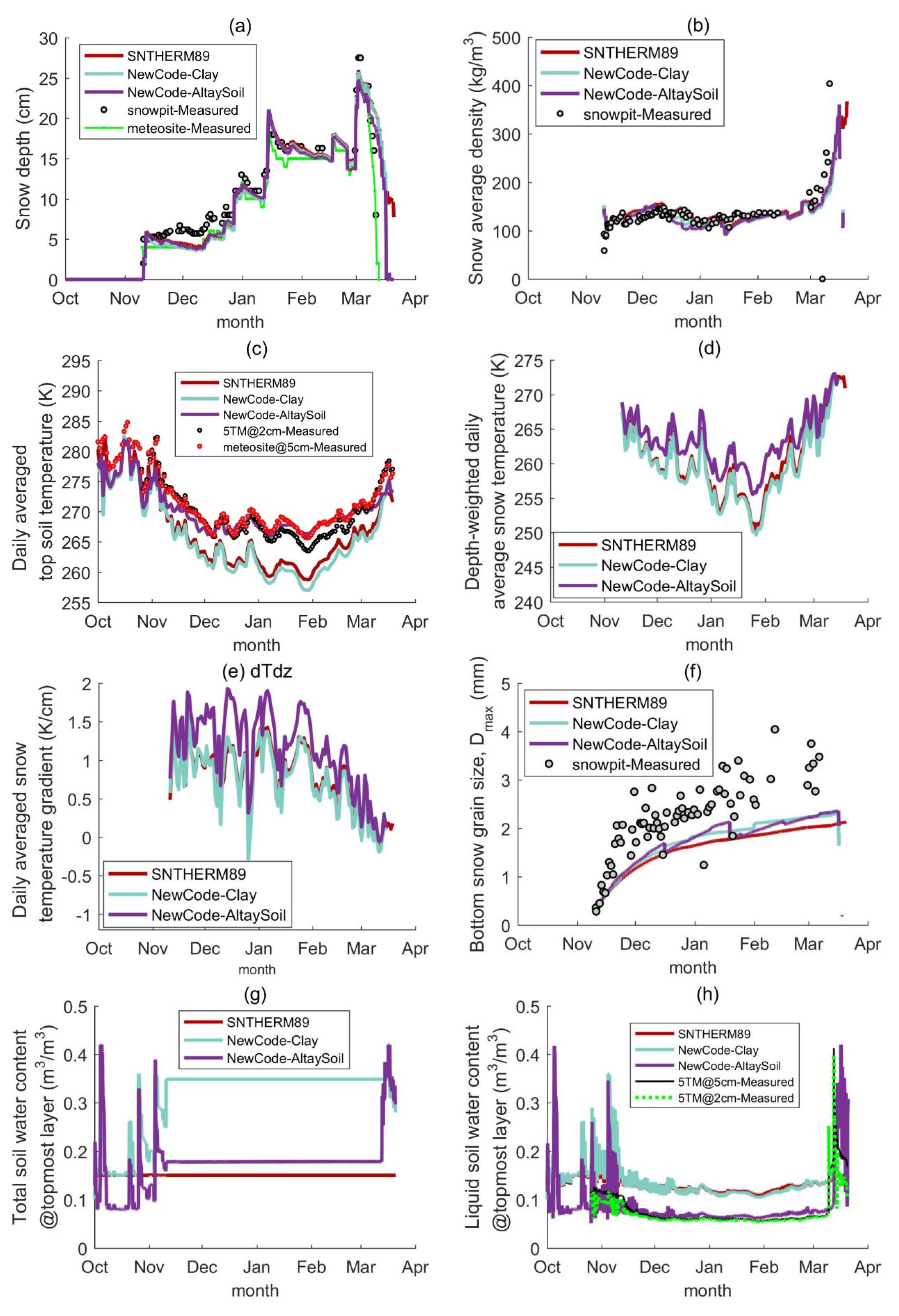
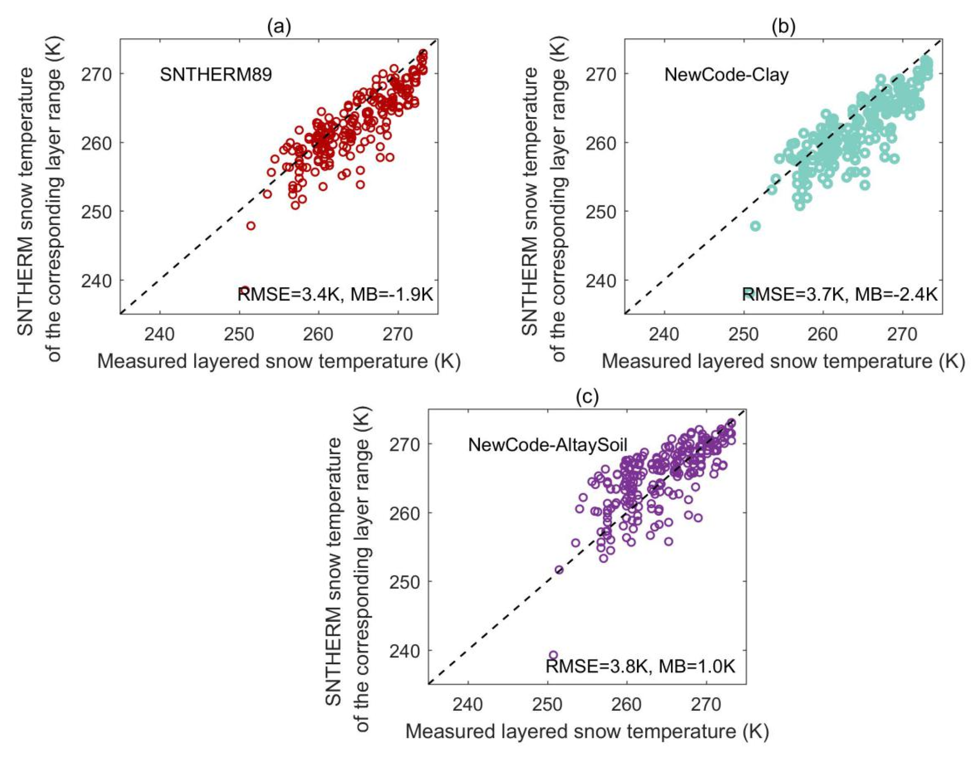
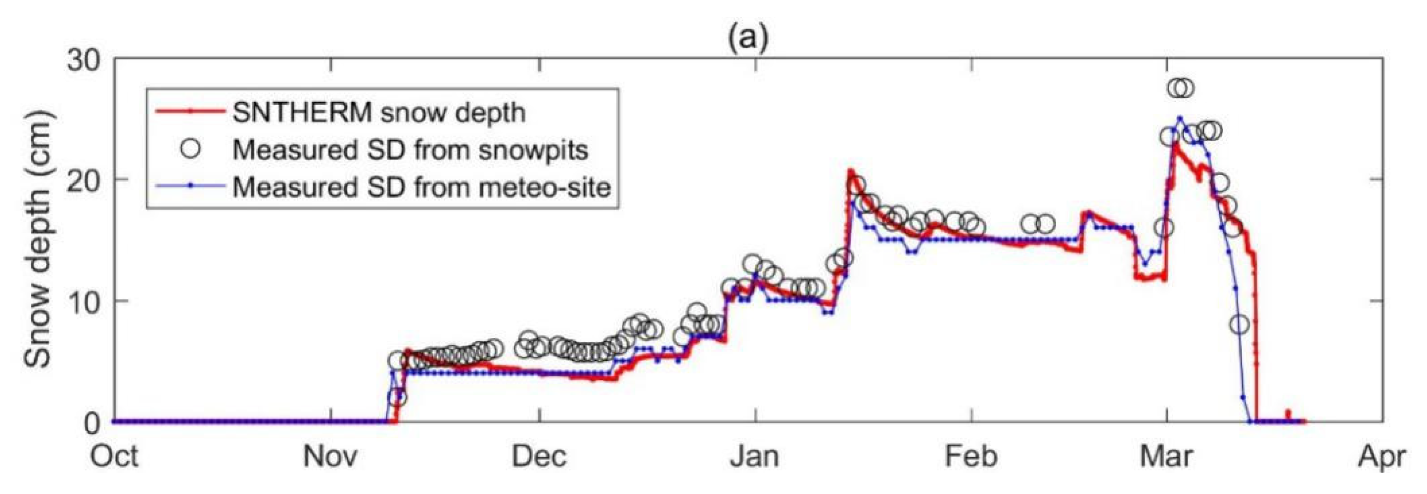
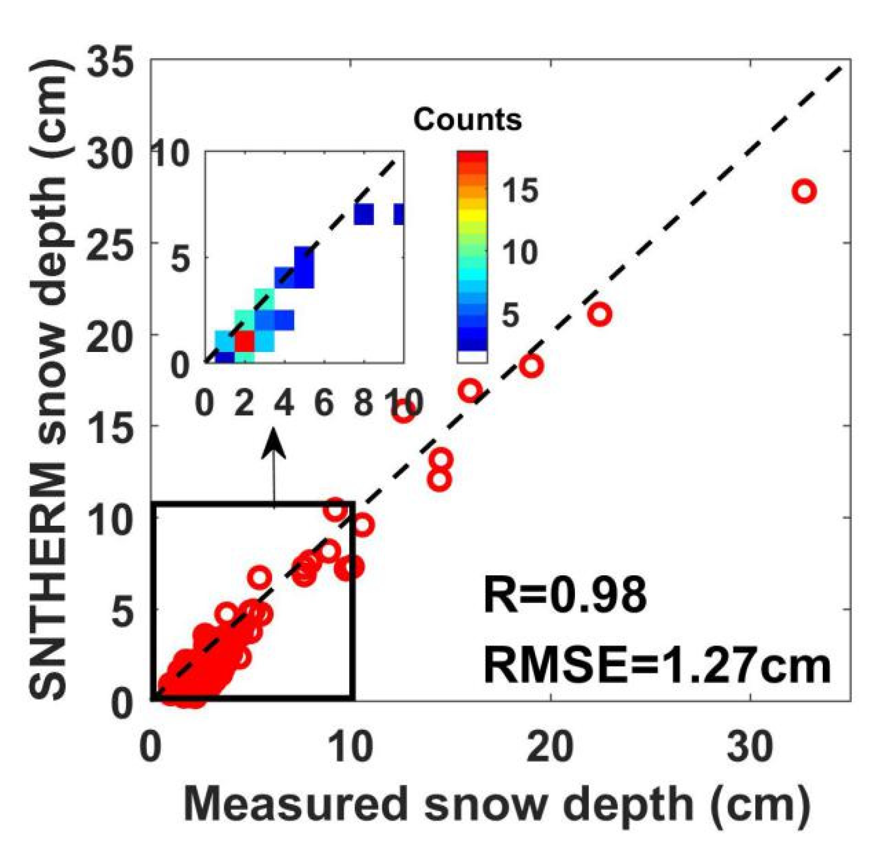
4.1. The Revised Soil Modeling in SNTHERM and the Validation Based on the Altay Experiment

Figure 4 shows a comparison of the simulated snow and soil state parameters using the original SNTHERM89 code (scenario 1) and the revised SNTHERM with the soil water movement considered (scenarios 2 and 3), driving by the same meteorological forcing data. The default g₁ of 5.0 × 10⁻⁷ m⁴/kg was utilized for simulation. Figure 4 also includes the field measurements if available. For the temperature variables, the daily-averaged mean values were plotted for a better presentation compared to strongly fluctuated hourly values.

From Figure 4a, it shows the simulated snow depth from three scenarios is close, except the original SNTHERM89 code gives a slower melt for the last few days. In the snow accumulation phase, the difference in the simulated snow depth based on different soil settings is tiny, in the magnitude of 0.7 cm in maximum. The simulated snow depth matches the observed snow depth. On the other hand, during the snowmelt phase, the simulated snow by scenarios 2 and 3 (NewCode-Clay and NewCode-Altay) completely melts on 22:00 and 21:00, respectively, March 16th, whereas the measurement from the meteorological site gives a first snow-free day on March 13th. The end of snow season simulated by SNTHERM delays by 3 days. It will be improved by correcting the bias in the snow grain size estimation, as will be shown later in Figure 8a.

In Figure 4b, the simulated average snow density is also close among 3 soil parameter scenarios, and matches the observations from the snowpits.

Figure 4c–e show the soil thermal properties influence the simulated topmost soil layer temperature (c), the average snow temperature (d), and the average snow temperature gradient ((T_snow,bottom − T_snow,top)/SD) (e). All the lines presented here are for daily average values. In Figure 4c, the daily average top soil layer temperature measured by the station and by our 5TM sensor are also added. It shows the use of the clay soil type (scenarios 1 and 2) underestimates the soil temperature for over 10 K in the coldest time. A significant improvement is observed by using the Altay site-specific soil type and a volumetric liquid water content of 20% for deep soil layers at the initial time. The simulation result using a homogeneous 10% volumetric liquid water content profile is between scenarios 1 and 3 (not shown here). Scenario 3 (NewCode-AltaySoil) gives a higher top soil temperature and because the topmost snow temperature approximates the air temperature, it gives a higher averaged snow temperature (Figure 4d) and stronger temperature gradient (Figure 4e). According to Equation (1), a higher temperature and temperature gradient can accelerate the grain growth speed. Therefore, scenario 3 predicted a slight higher bottom geometric snow grain size (D_max) in Figure 4f, but is not always higher for all days compared to scenario 2. However, the diversity in D_max is not as strong as we speculated. The resulted diversity in the predicted brightness temperature will be discussed in Section 5.1.

Figure 4f shows all three scenarios underestimated the observed D_max from the snowpits. In order to support the update of grain growth coefficient (g₁), an accurate estimation of the snow temperature and snow temperature gradient is the prerequisite condition. In Figure 5, the calculated and the observed temperature gradient from snowpits are compared. The later was calculated by the difference of snow temperature divided by the difference of the measured heights ($-\partial T/\partial z$). It shows the simulated temperature gradient has a strong diurnal variation—low in the daytime and high in the night time. The highest temperature gradient can reach 2 K/cm, whereas that at noon it is in general around 0.5 K/cm or can even be negative. Two reasons resulted in a measured smaller temperature gradient compared to the simulations. First, most measurements of snow temperature were at the daytime, and reasonably it reaches the low limit of the simulations. Second, the measured temperature of the bottommost snow layer can be biased low. The insertion of the temperature sensor easily broke the sugary depth hoar at the bottom and can mix cold air into the snow around the sensor. We think the temperature of the topmost soil layer is a more reliable validation reference than the bottom snow temperature measurements. Figure 6 compares the instant snow layer temperature and the SNTHERM snow temperature. It showed the temperature using the clay soil (scenarios 1 and 2) biased low for 2 to 3 K. The prediction using the Altay site-specific soil (scenario 3) is better. As a conclusion, the temperature simulation using scenario 3 improves over scenarios 1 and 2, and can be used for the grain growth coefficient adjustment.

Figure 4g,h show the simulated total water content and liquid water content for the topmost soil layer. In Figure 4g, the total water content using SNTHERM89 nearly changes due to model defect as speculated. When the soil water movement is added, both the scenario 2 using clay soil and the scenario 3 using Altay site-specific soil can reach the saturated volumetric water content (0.36 for scenario 2 and 0.42 for scenario 3) after snowmelt or a rainfall. However, the drainage of the Altay soil is quicker than clay. In combination with a slower freezing speed, the Altay soil type gives a smaller total water content during the snow-covered days. We had some total gravimetric water content (m_g) measurements from drying the extracted soil sample by the oven. The measurements showed 9–12% m_g in the 0–4 cm depth between November 7th to 16th. It was around 5% m_g after November 22nd; however, after the soil was frozen, a representative sample was difficult to take. The measurements in mid-November indicate that the simulation using Altay soil is more plausible.

From Figure 4h, it shows the temperature has a strong influence on the liquid water content. Scenarios 1 and 2 give similar simulations because their simulated soil temperature is close and the soil freezing curve parameter (plasticity index) is the same. The plasticity index of Altay soil was adjusted to match the 5TM observed equivalent liquid water content.

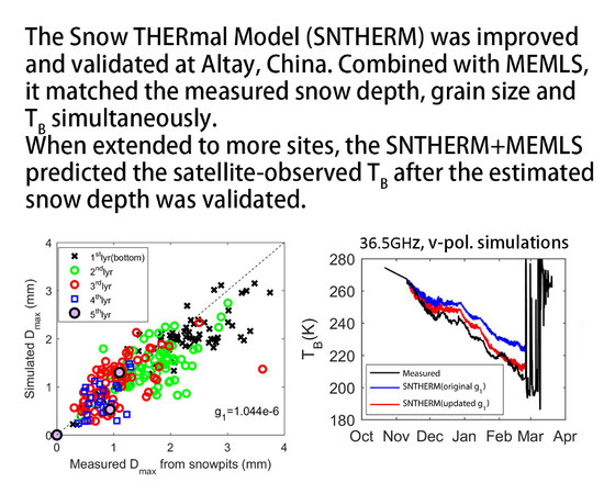
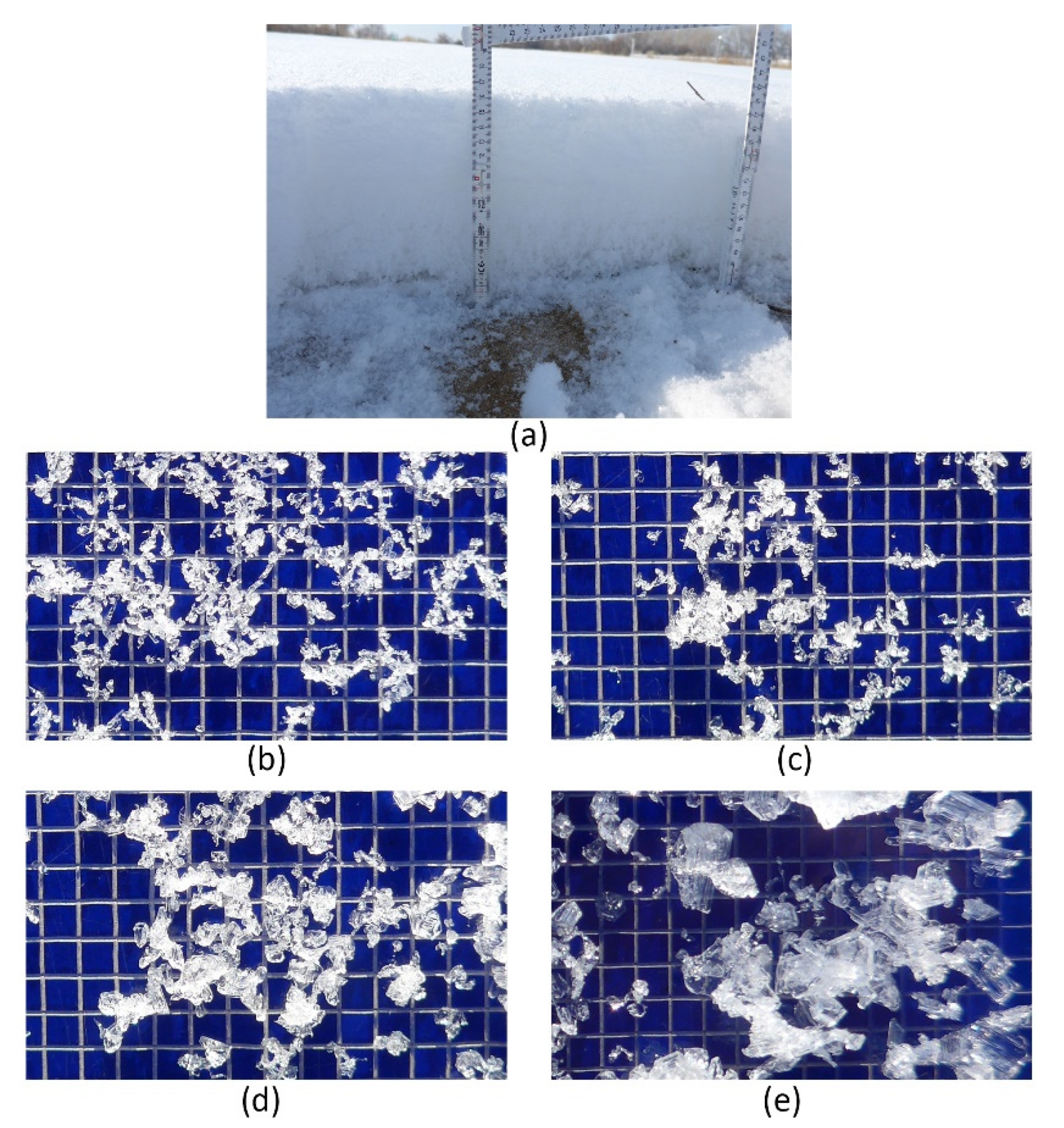
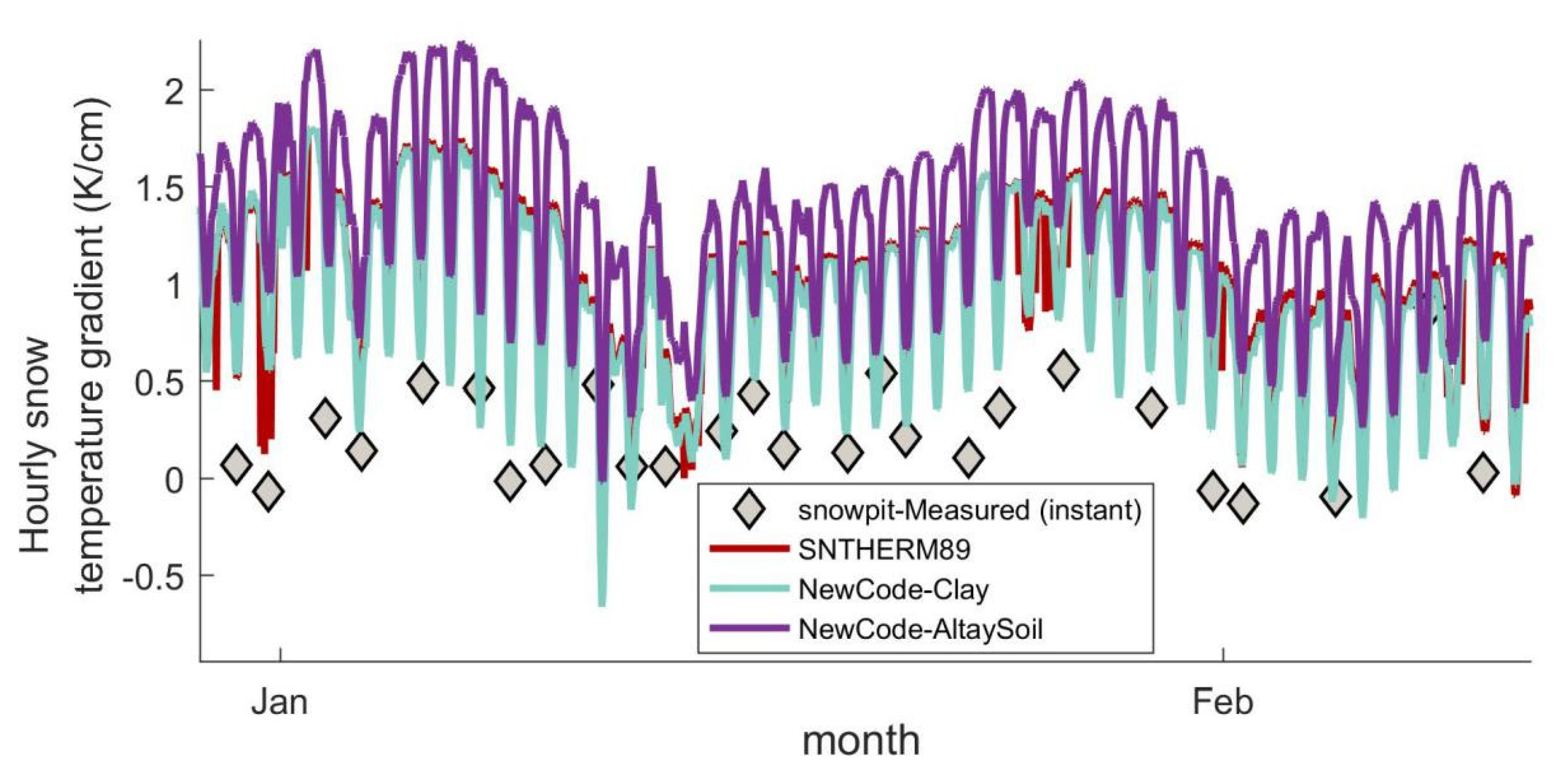
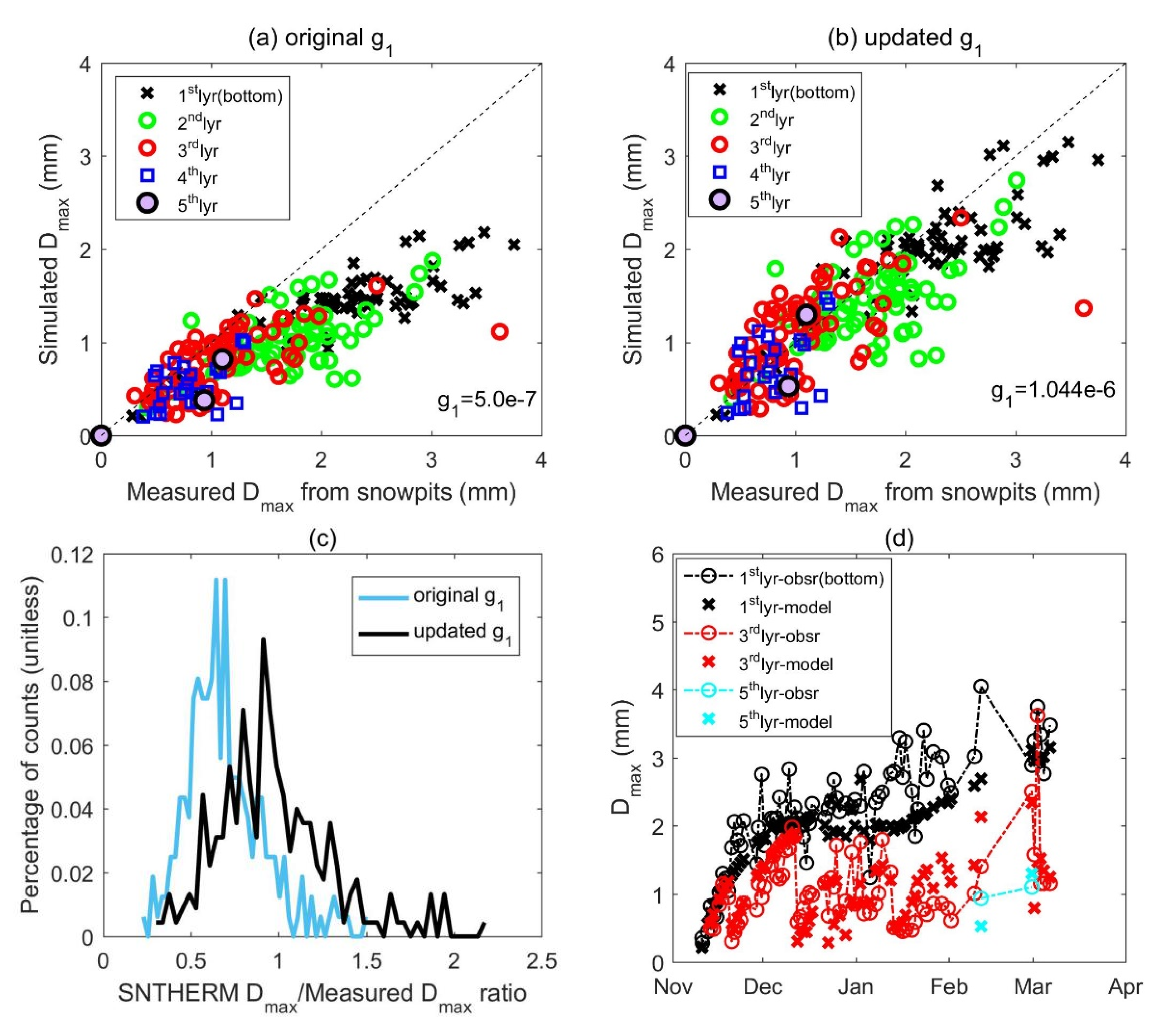
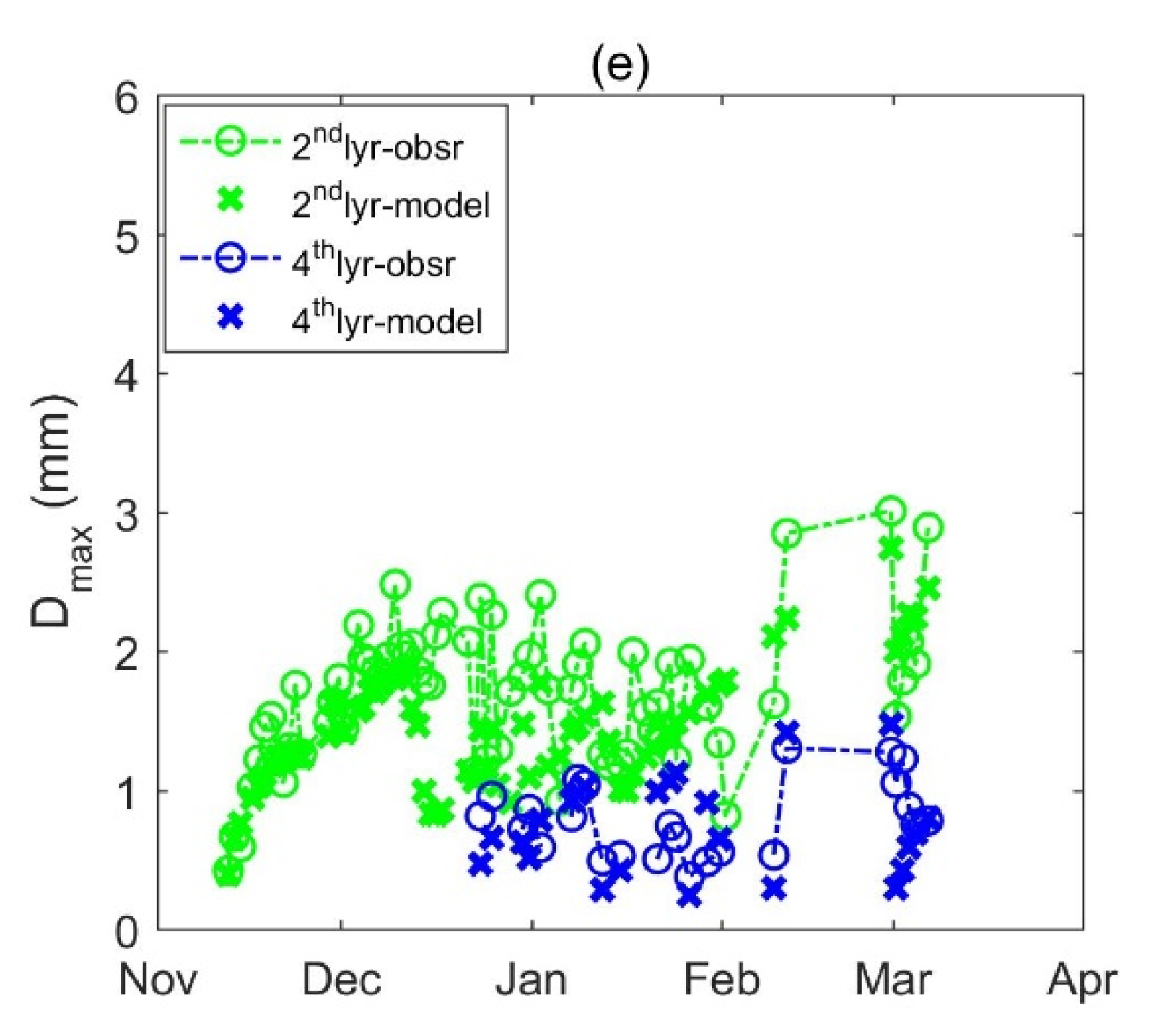
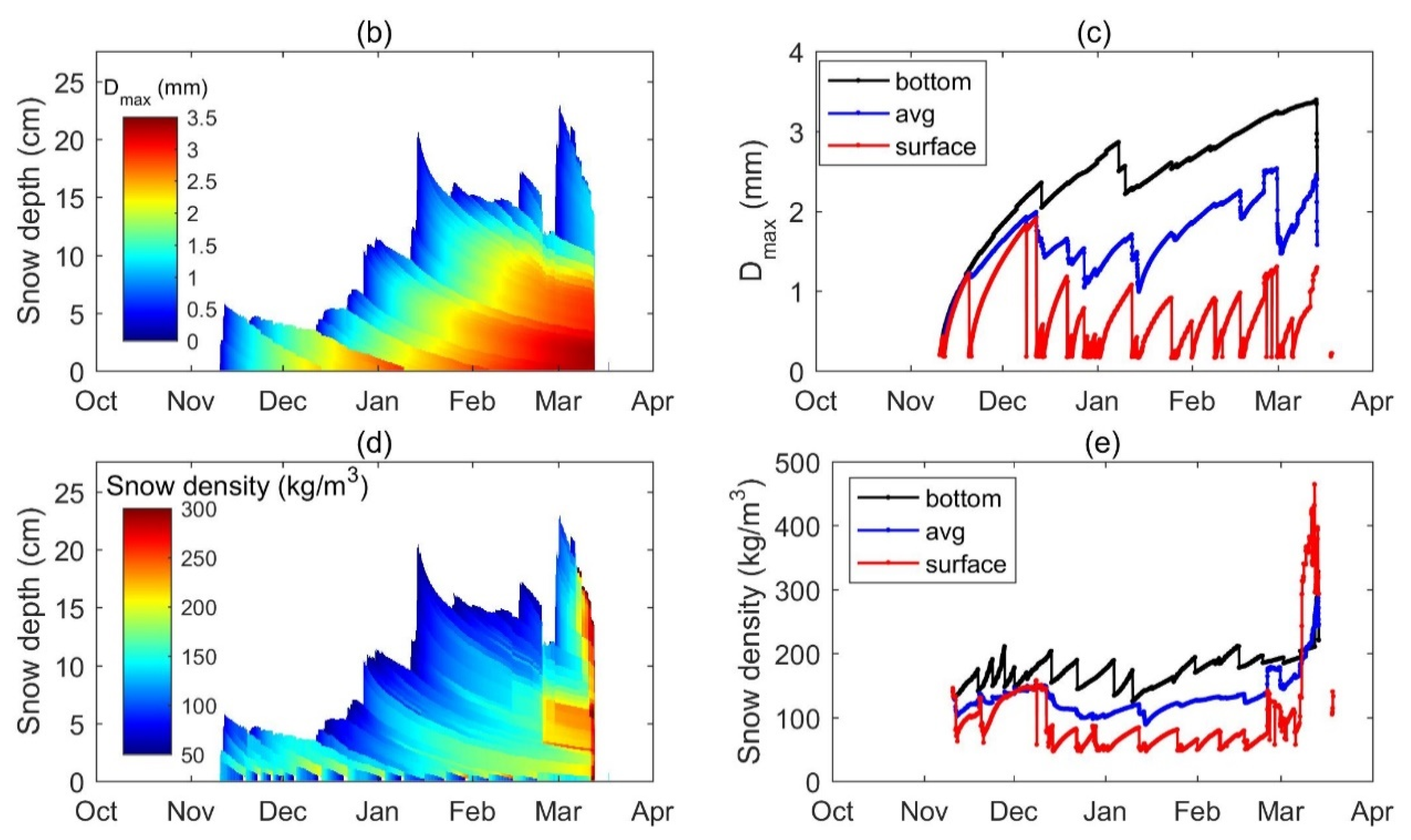
4.2. The Grain for the Altay Experiment

After the snow temperature and the temperature gradient were accurately provided using the Altay site-specific soil parameters, the next step is to improve the grain growth coefficient (g₁). In Figure 7a, the simulated D_max from scenario 3 is plotted against the measured D_max from the snowpits. The SNTHERM simulated much more snow layers (1–34 layers) compared to the in-situ measurements (1–5 layers). Here we extracted the SNTHERM snow layers within the height range of the snowpit layer and took the average. Currently, using the default g₁, the simulated D_max biased low, for about −0.55 mm in average (RMSE = 0.74 mm). The ratio of the simulated to the measured D_max is 0.69 ± 0.22.

Assuming the geometric grain size at time (t) = 0 is d₀, Equation (1) has an analytical solution as:

$$d=\sqrt{2g_1\left|U_v\right|\Delta t+d_0}$$

(10)

Because the model was run before the first snowfall, it called an empirical function to calculate the fresh snow density and used the fresh snow density to calculate d₀. d₀ is 0.16~0.17 mm for a fresh snow density of 50~200 kg/m³; it makes d₀ negligible in Equation (10). As a result, to scale d by a factor of b approximately equals to multiplying g₁ by a factor of b². b = 1/0.692 = 1.445. Therefore, an improved g₁ should be 5.0 × 10⁻⁷ m⁴/kg * 1.445 × 1.445 = 1.044 × 10⁻⁶ m⁴/kg.

Figure 7b showed the D_max comparison using the updated g₁. After revision, the mean bias is reduced to −0.15 mm (RMSE = 0.47 mm). The ratio of the simulated to the measured D_max is changed to 0.97 ± 0.33. By changing g₁ to match the observed geometric grain size, a well-defined physical meaning is introduced to the SNTHERM snow grain size, which was previously considered as a model-specific, effective grain size. Figure 7c presented a comparison of the histogram of the simulated to measured D_max ratio. Figure 7d,e showed more details of the time-series varied D_max trend at different layers in the bottom-first order.

After the grain growth coefficient (g₁) was updated, the simulated snow depth and geometric grain size and density profiles are presented in Figure 8. In Figure 8a, after the g₁ was improved, the simulated snow melts on 23:00 March 13th, 2018. Comparing with the measured snow-free day on March 13th (daily scale), the error is within one day. The new simulation has been significantly improved over the originally-simulated March 16th. It demonstrated that, after the grain size is accurately predicted to higher values, the snow albedo is reduced to promote a quicker snow melt. In Figure 8a, the snow depth prediction accuracy is −1.49 cm mean bias (MB) and 1.91 cm root-mean-squared-error (RMSE).

Figure 8b,e show the snow grain size and the snow density profiles. In Figure 8c,e, depth-weighted average values and the values at the surface and the bottom of the snow are presented. The fluctuation of the surface layer geometric grain size and density is due to new snowfalls. After a snow layer is initialized from a new snowfall, in theory, the snow grain size monotonically increases. However, the combination of snow layers can reset the simulated values. For the bottom snow layer, two reasons from the model numerical implementation can result in a decreased snow grain size and density. Firstly, when the bottom layer is compressed to a thickness smaller than the limit, the bottom-most layer will be combined with the 2nd bottom layer and the snow parameters are averaged. Such fluctuations can also be found using the SNTHERM89 code. Secondly, the bottom snow mass can be reduced in SNTHERM via the water vapor movement, and this can result in a ‘disappearance’ of the bottom layer.

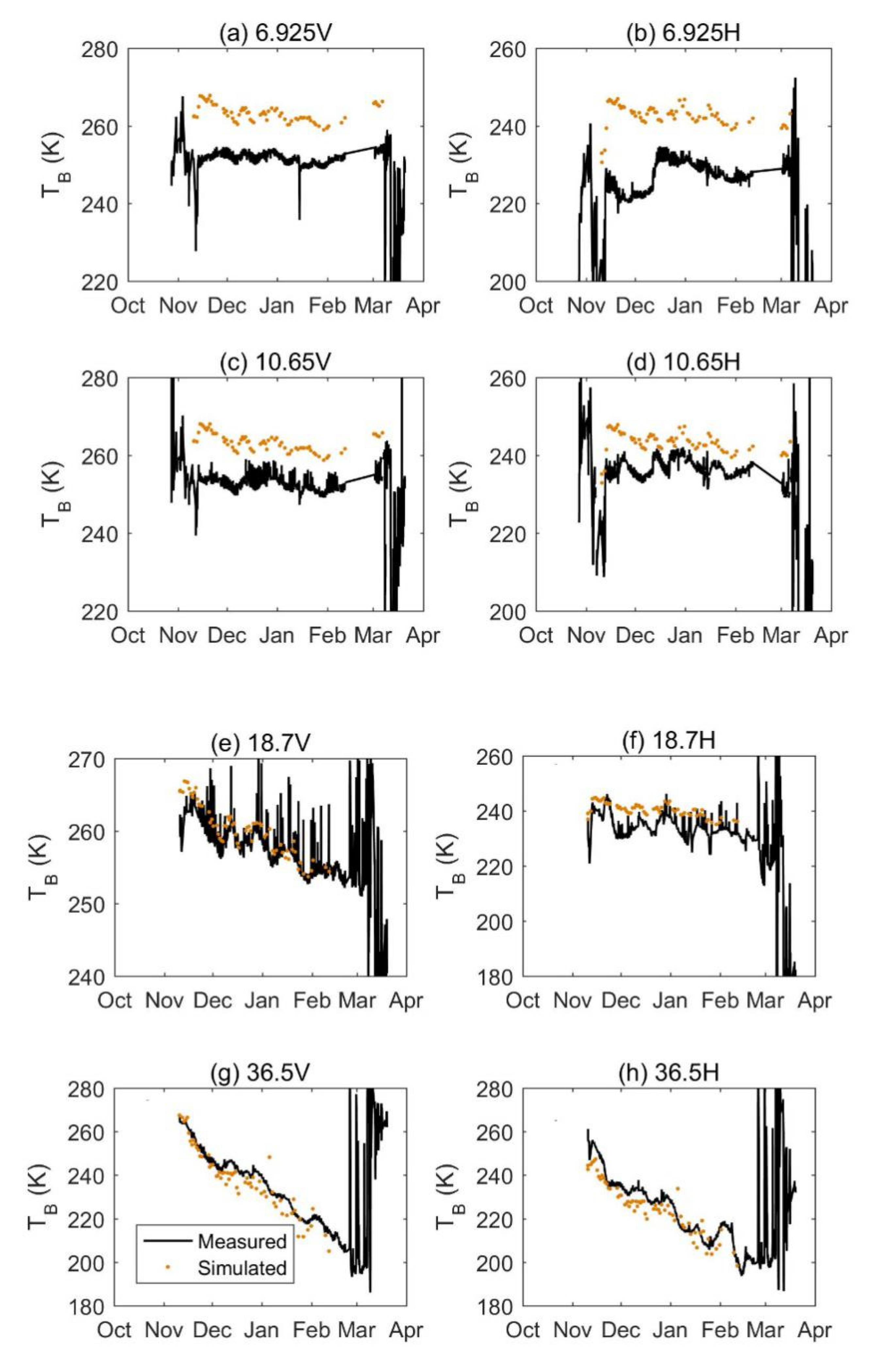
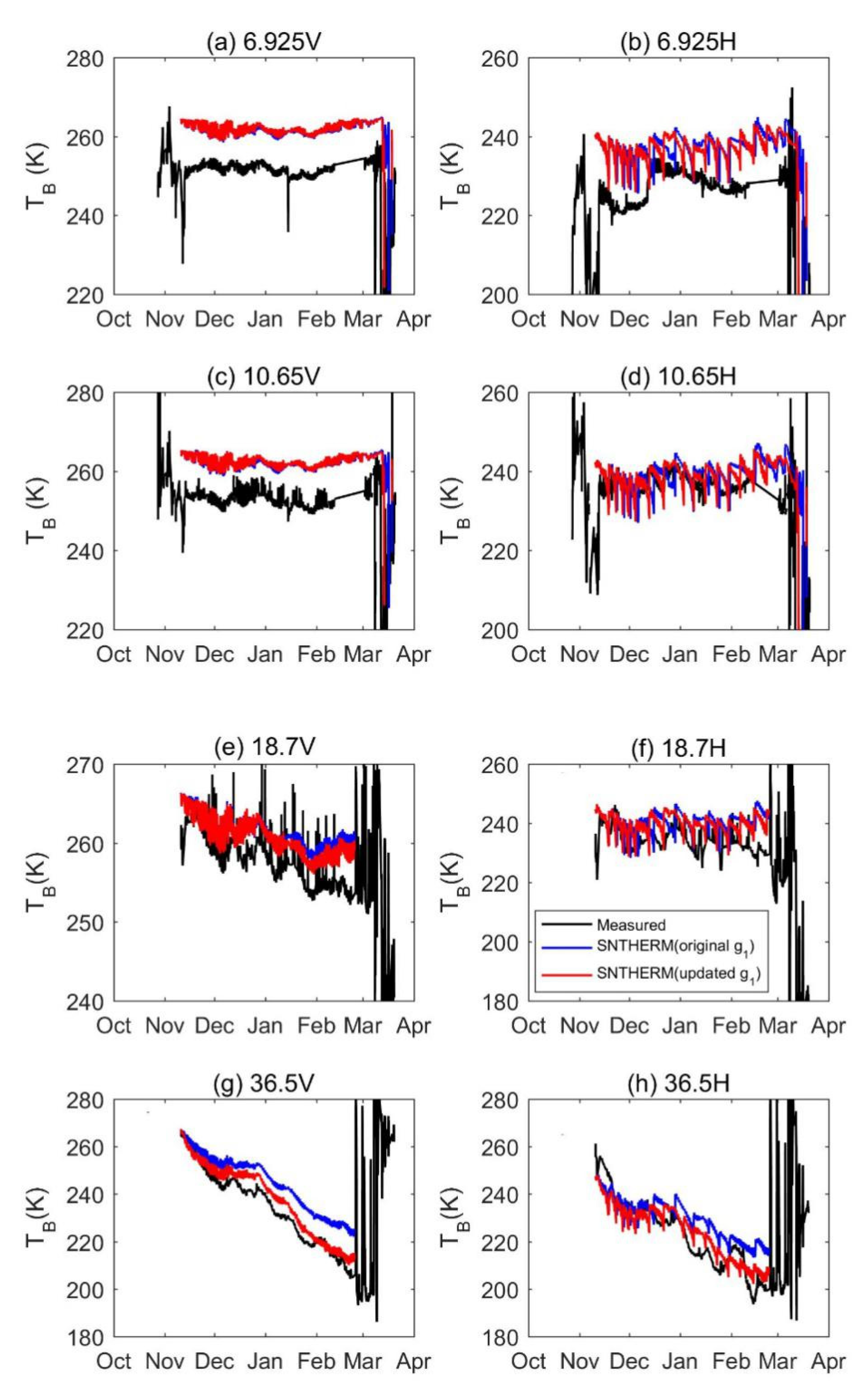
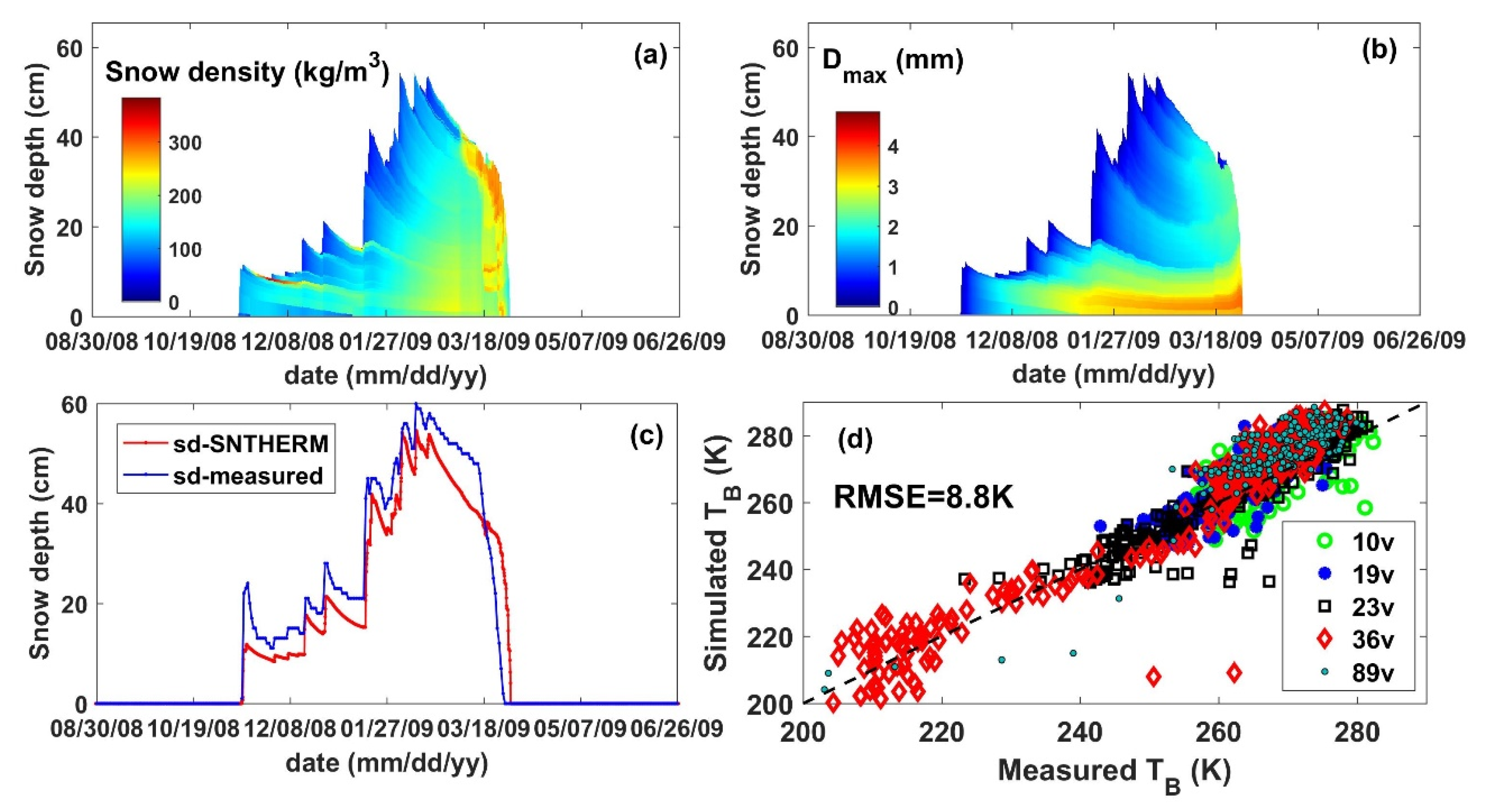
4.3. Brightness Temperature Simulation for the Altay Experiment

Figure 9 shows the comparison between the ground-based radiometer measured and the MEMLS simulated T_B at 6.925, 10.65, 18.7, and 36.5 GHz, dual polarization, using the snowpit measurements (including layer thickness, geometric grain size, density, and temperature) and the soil parameters at −2 cm depth from the Decagon 5TM sensor. Figure 10 is the comparison result using all snow and soil parameters from the SNTHERM simulations. Here we utilized the D_max to p_ex coefficients in Equation (8). The soil reflectivity was modeled using a fixed soil roughness of 2 cm for all cases.

An error statistic is shown in

Table 2. Error statistics of the simulated brightness temperature in the Altay experiment compared with ground-based radiometer measurements.

Error (K)	6.925 V	10.65 V	18.7 V	36.5 V	6.925 H	10.65 H	18.7 H	36.5 H
Simulated using snow pit measurements	11.32	9.71	2.56	5.54	16.96	7.30	8.07	6.11
	(11.12)	(9.45)	(1.86) 1	(−3.16)	(16.25)	(6.70)	(7.51)	(−3.51)
Simulated using SNTHERM predictions with updated g1	10.58	9.75	3.24	4.43	11.85	5.30	7.40	6.37
	(10.30)	(9.59)	(2.75)	(3.37)	(10.46)	(2.55)	(5.91)	(0.95)
Simulated using SNTHERM predictions with original g1	10.30	9.52	3.88	10.95	11.97	5.76	8.26	10.29
	(9.99)	(9.34)	(3.35)	(10.04)	(10.58)	(2.78)	(6.56)	(6.52)

¹ The errors are formatted as: RMSE (MB).

. It shows using the snowpit measurements, the root-mean square error (RMSE) of the brightness temperature at 18.7 V, 36.5 V, 18.7 H, and 36.5 H are 2.56 K, 5.54 K, 8.07 K, and 6.11 K, respectively. The mean bias (MB) is 1.86 K, −3.16 K, 7.51 K, and −3.51 K, respectively. Figure 10 shows the comparison using the SNTHERM simulated parameters based on both the original default g₁ and the updated g₁. It shows the updated g₁ corrected the overestimated T_B from the original g₁. The difference is stronger at the end of the snow season when both the snow depth and the grain size is higher to become sensitive to the microwave volume scattering. It implies an important point that, because SNTHERM snow grain size monotonically increases with time, the simulation of snow particles needs to be very careful to prevent “over-growth” at the early stage when the T_B is still not sensitive. Table 2 also shows the RMSE and MB using the updated g₁ are of the same level with the simulation using the snowpit measurements.

As a summary, using the Altay experiment data, we managed to simultaneously match the observed snow depth, snow grain size and brightness temperature. Our validation reconfirmed the D_max to p_ex conversion coefficients and suggested an increase of the grain growth coefficient by 2.088 times. The same parameter values will be used for simulations at 102 stations in the next section.

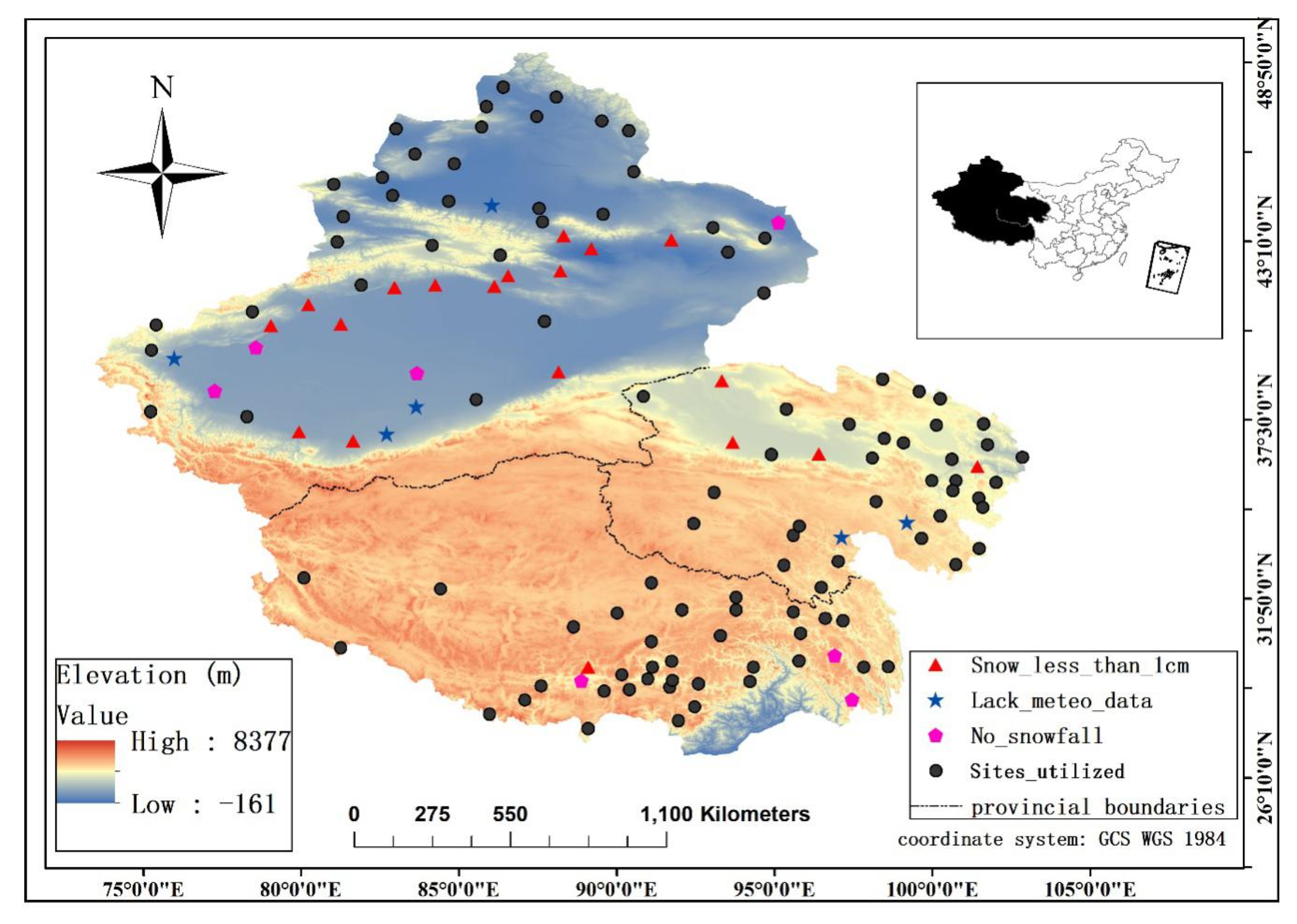
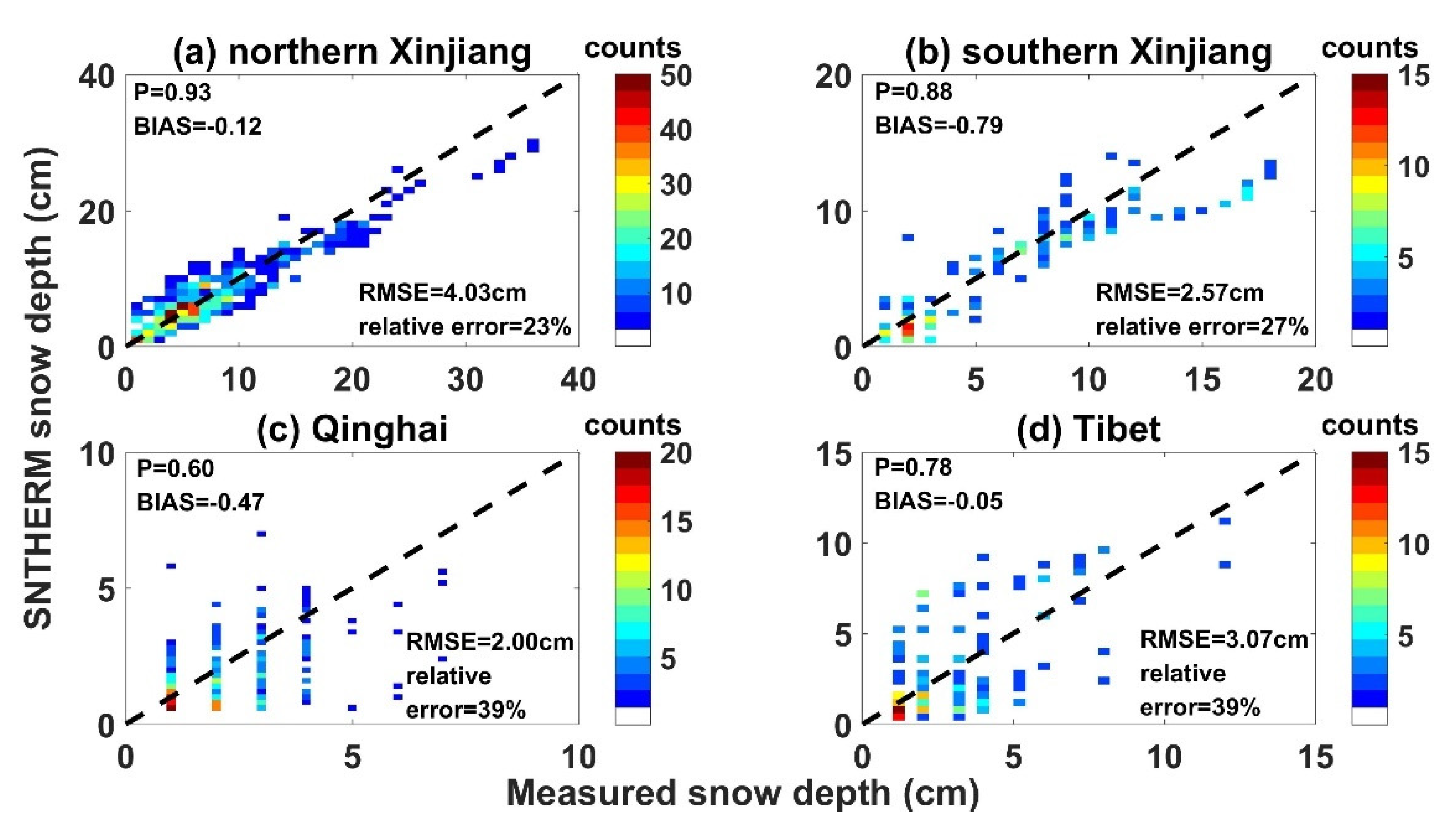
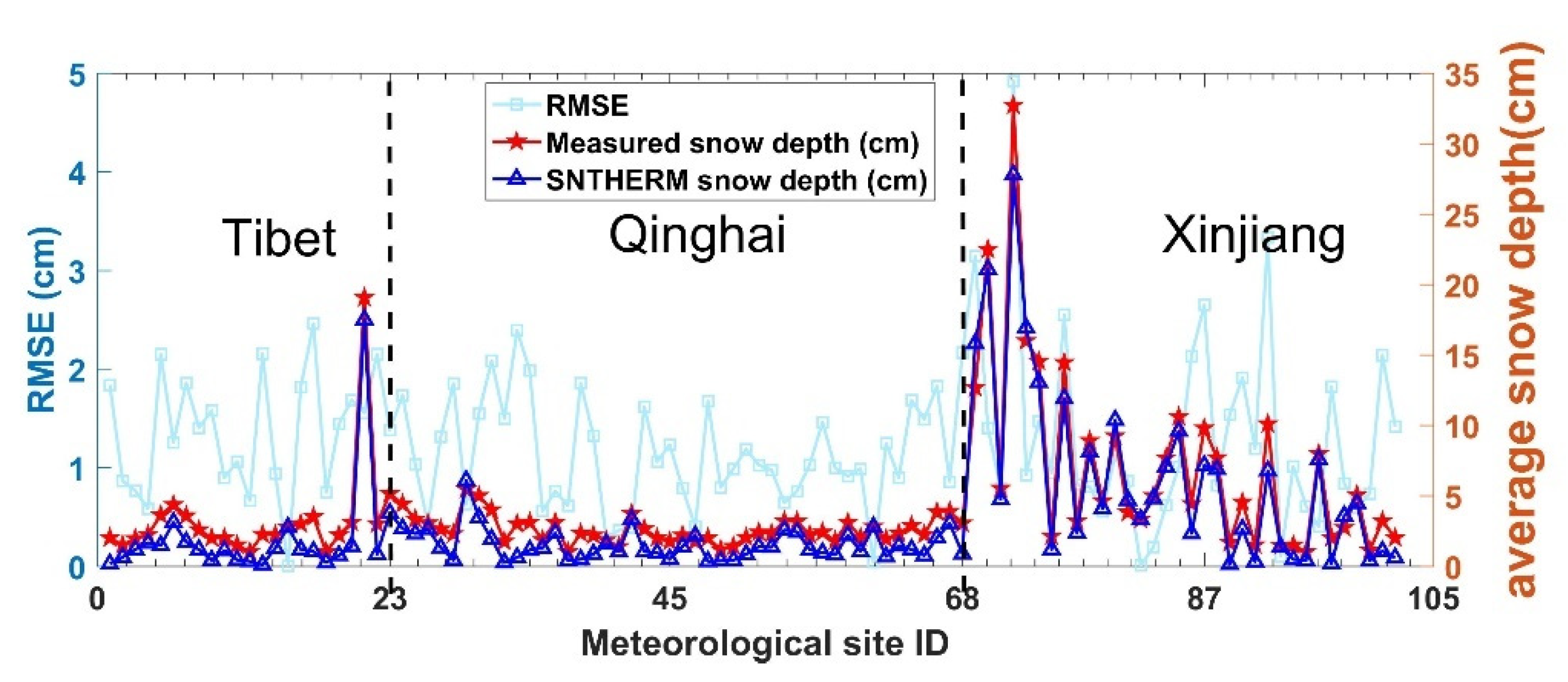
4.4. Validation of Snow Depth at the 102 Sites

Figure 11 shows the comparison of daily measured snow depth from the 102 meteorological stations in the 2008–2009 winter with the SNTHERM simulations. The result is presented into 4 subplots, for 4 different regions. The points for northern Xinjiang and southern Xinjiang are separated due to strong snow depth difference. The snow depth RMSE is 4.03 cm in northern Xinjiang, 2.57 cm in southern Xinjiang, 2 cm in Qinghai, and 3.07 cm in Tibet, respectively.

Figure 12 and Figure 13 show the statistics of average snow depth among the 2008–2009 snow season; Figure 13 additionally shows the statistics of daily snow depth estimation RMSE at each station. It shows that in most stations, the average snow depth is below 5 cm in the Tibet and the Qinghai provinces, but is much higher in the northern Xinjiang. The accuracy of the seasonal average snow depth is 1.27 cm RMSE and 0.98 correlation (R). The simulated snow depth is slightly biased low. The relative error is lower in northern Xinjiang where a deeper snowpack develops.

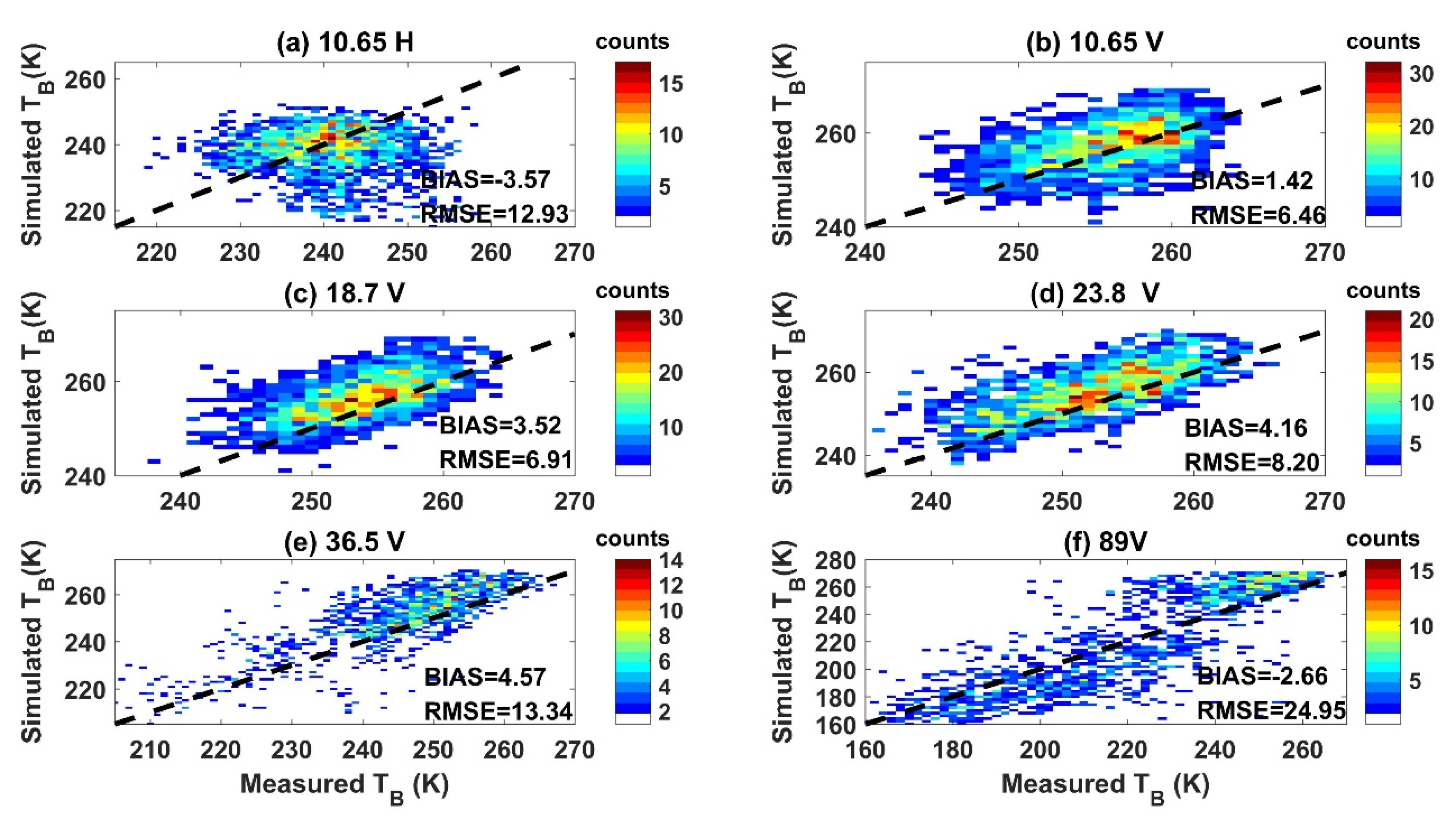
4.5. Validation of the Brightness Temperature at the 102 Sites

Snow microstructure is the key parameter to influence the brightness temperature in snow. After the snow depth is validated, the SNTHERM simulated snow and soil parameters were inputted to MEMLS to calculate the pixel-scale brightness temperature and to compare it with the AMSR-E observations from the descending orbit (1:30 a.m. local overpass time, approximately). To reduce the influence of wet snow condition, the error statistics use the period from December to February in the next year.

Figure 14 is an example of brightness temperature validation at the Altay station in the 2008–2009 winter. In this winter, the Altay station had a maximum snow depth of 60 cm. The T_B at 10.65 GHz, 18.7 GHz, 23.8 GHz, 36.5 GHz, and 89 GHz, vertical polarization, was simulated with an overall RMSE of 8.8 K, from daily-based statistics.

Figure 15 shows the comparison of measured and simulated daily T_B at all stations. The agreement is higher for frequencies larger than 10.65 GHz. The RMSE is 6.91 K, 8.2 K, 13.34 K at 18.7, 23.8 and 36.5 GHz, vertical polarization, respectively. At 10.65 GHz, the correlation between the measured and the simulated T_B is smaller, whereas the RMSE is 6.46 K and 12.93 K at vertical and horizontal polarization, respectively. The simulation at this frequency is influenced strongly by the soil modeling beneath the snow. We utilized the same soil parameters as in the Altay experiment, so the accuracy will be reduced. More important, usually the underlying background beneath the snow cover in the pixel scale is different with the bare soil assumption. For Figure 15a,b, we did not correct the time independent offset sometimes found between the simulated and the observed T_B time series caused by the soil modeling and the complex land surface conditions, which may be considered as a systematical bias like in Figure 9 and Figure 10. The largest RMSE (of 24.95 K) is found at 89 GHz because this frequency is very sensitive to the grain size of the topmost snow layers. A good point is the simulated T_B is unbiased in 160–200 K range. The T_B above 200 K is biased higher, which indicates a possible underestimation of new snow grain size using the SNTHERM inner computation module instead of a user-defined value. The small 89 GHz T_B measurements occurred when the snow crystals at the snow surface has grown large, before the next new snowfall.

5. Discussions

5.1. Analysis of the Influence of Soil Parameter Setting on the Brightness Temperature Simulation

Section 4.1 demonstrated that the setting of soil parameters influences the snow temperature, temperature gradient, and therefore influences the calculated grain size, according to the SNTHERM model theory. In Figure 4c and Figure 6, it shows the use of a site-specific Altay soil type predicts the temperature variables better. In Figure 4f, the simulated bottom D_max is in average slightly larger using the Altay site-specific soil (dark purple line) compared to clay (light blue line). The influence will be enlarged after the grain grow rate is increased. Therefore, here we added a discussion to evaluate the soil parameter influence on the T_B simulation at 36.5 GHz. The T_B is a more significant impact indicator compared to layered D_max in small values.

Figure 16 shows the comparison of T_B using two different SNTHERM simulated soil properties (a) and the same property from 5TM soil sensor measurements (b). In Figure 16a, it shows surprisingly, the simulated T_B is better using the original clay soil setting. The error is most likely from the soil dielectric constant modelling. By comparing with Figure 16b, it shows the reason is from the difference in the simulated soil properties caused by different soil parameter settings, not from the simulated D_max difference in Figure 16c. In Figure 16c, it showed the average D_max using Altay soil is still larger than the clay soil, which agrees with Figure 4f and the modeling theory; however, in the mid snow season, the bottom layer D_max using clay soil can be reversely larger, due to the randomness in layer combination.

Table 3. Difference in the Altay experiment simulation using clay and site-specific soil parameters.

Difference (Clay−AltaySoil)	Average Difference	Maximum Difference
Difference in 36.5 V TB caused by soil parameter inputs	−5.18 K	−9.98 K
Difference in 36.5 V TB caused by the influence of soil parameter inputs on Dmax	0.78 K (with difference in average Dmax: −0.09 mm; bottom Dmax: 0.1 mm)	4.66 K (with difference in average Dmax: −0.27 mm; bottom Dmax: 0.51 mm)
Difference in 36.5 V TB caused by different g1 *	6.93 K	14.06 K

* The baseline is SNTHERM simulated snow properties using Altay soil setting and the soil parameters from 5TM sensor measurements.

compares the T_B difference caused by different soil parameter settings, by the influence of soil parameter settings on the simulated snow grain size (with soil property difference excluded) and by the different grain growth coefficients (the original and the revised g₁). It shows the influence of grain growth coefficient correction is strongest (of 6.93 K in average), indicating its importance. The influence of soil property simulation accuracy is in the second order, with a magnitude of 5.18 K in average, but its maximum influence is within 10 K. The influence of soil parameter setting on the geometric grain size prediction is in the order of 0.1 mm in average, and the resulted T_B difference at 36.5 GHz, vertical polarization is within 1 K in average. It implies the SNTHERM simulated snow properties are trustable regardless of the soil parameter setting.

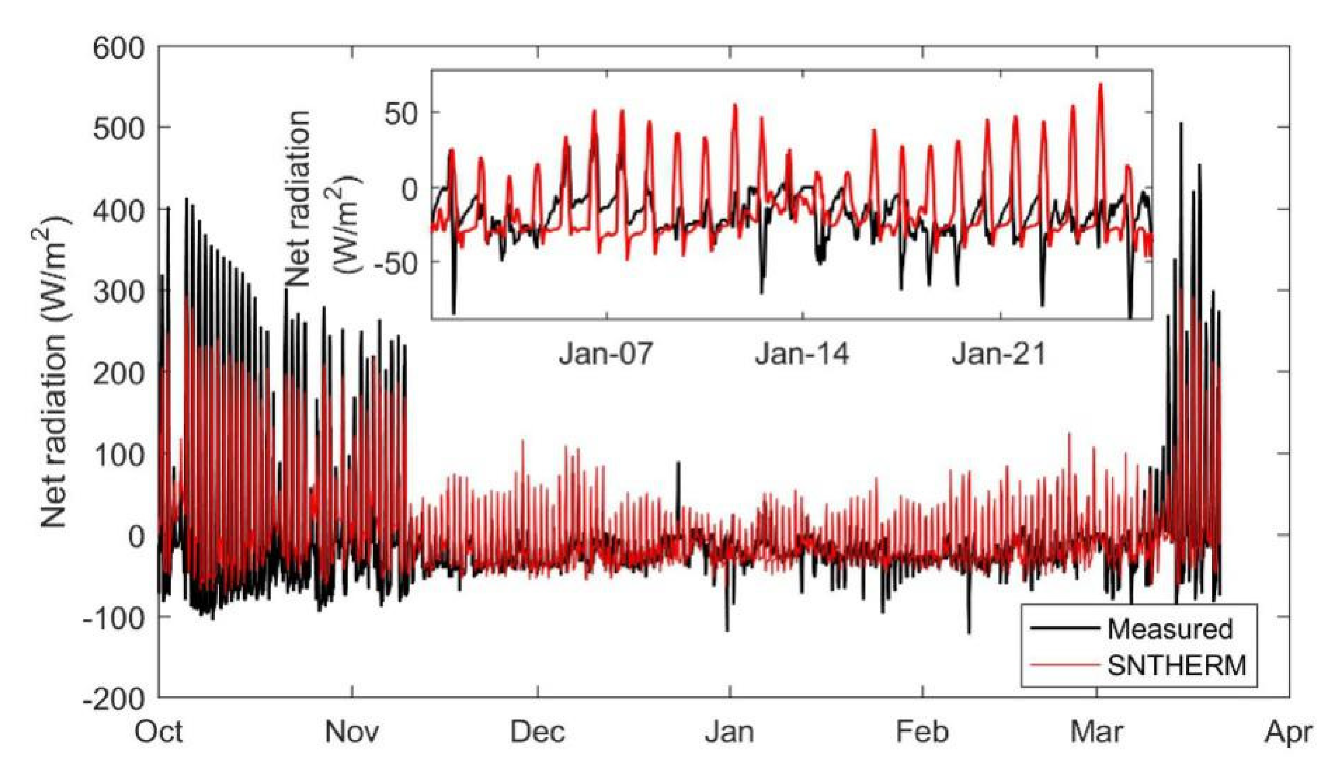
5.2. Evaluation the Use of GLDAS Downwelling Longwave Radiation

In Section 2.1, we mentioned the downwelling longwave radiation inputted to the SNTHERM model is from the GLDAS dataset. The station does not have the downwelling longwave radiation measurement. We didn’t force the simulated net radiation to match the observed net radiation, because we considered the difference between the SNTHERM model pure snow assumption and the in-situ condition influenced by the dry high grass. A natural condition is required by the meteorological station observation; however, as seen from Figure 17, the measured net radiation has a smaller peak at noon, influenced by the low albedo and the shade from the dry high grass.

Averaged from the November 10th, 2017 to March 12th, 2018 snow-covered period, the SNTHERM simulated net radiation on pure snow is 9.84 W/m² higher compared to the measurements from the meteorological site; the hourly standard deviation of difference is 31.15 W/m².

5.3. Error Analysis for the Brightness Temperature Simulation at 102 Stations

The accuracy of the brightness temperature simulation at the 102 stations is influenced by the following reasons. Firstly, the snow grain size was not directly validated on the Tibetan Plateau, its prediction accuracy still needs more exploration. Secondly, the soil hydraulic and thermal parameters were not set using local datasets. Although we have shown that the influence of soil setting on snow parameter estimation is limited, the soil parameters can still change the background emissivity beneath the snow and influence the T_B simulation; it was about 10 K in Altay experiment. Thirdly, the background condition of each pixel, which is in most cases mixed pixel at the AMSR-E resolution, is much complicated compared with the SNTHERM assumption. We had partly considered its influence by introducing the background emissivity and the fractional snow cover inputs. However, several factors were still not included, like the forest over the snow, the accelerated snowmelt from the warm grass under the snow, the different freeze-thaw evolution process of other land cover types in the mixed pixel, terrain effect on microwave modeling, terrain effect on snowdrift by winds, error in the satellite passive microwave observations, etc. These factors are the potential error sources for our simulation result in Section 4.5.

6. Conclusions

In this paper, we validated the use of the SNTHERM combined with MEMLS to simulate the snow depth, snow grain size, and brightness temperature in the Xinjiang, Qinghai, and Tibet provinces in China. Results showed that the SNTHERM has a good daily snow depth estimation accuracy, in the order of l–4 cm, when the accurate meteorological forcing is provided. During the Altay experiment, comparison with the in-situ measurements shows that the snow grain size can be predicted by an RMSE of 0.47 mm and mean bias (MB) of −0.15 mm. The simulated daily brightness temperature at 36.5 GHz, vertical polarization, has an accuracy of 4.43 K RMSE using the coupled SNTHERM and MEMLS model at the point-scale by comparing with the ground-based radiometer measurements from the Altay field experiment and 13.34 K using the AMSR-E observed T_B from the 102 meteorological stations of varied snow, soil property and mixed-pixel background characteristics. The statistics is based on the dry snow period from December to February.

Using the field experiment of the entire winter, we updated the grain growth coefficient (g₁) of the SNTHERM, and suggested a new value of 1.044 × 10⁻⁶ m⁴/kg. After this revision, we linked the SNTHERM predicted snow grain size to the geometric grain size definition that can be observed in the field.

The snow is very different on the Qinghai-Tibetan Plateau (QTP), compared to the northern Xinjiang. Driven by high solar radiation, the snow is easier to melt on the QTP and the snow depth is shallower in flat areas. The brightness temperature for shallow snow is easier to be influenced by other nuisance parameters, especially the background emission and the signals from other land cover types. Therefore, an extended field experiment is suggested in this region to validate the geometric grain size directly. The SNTHERM snow grain size was found to be biased in previous studies [34], whereas in this paper, this bias was corrected before the snow grain size was inputted to the snow brightness temperature modelling. Used together with the snow temperature and the snow temperature gradient, the grain growth rate g₁ of SNTHERM reduces its dependency on the other snow variables and has the potential to become a relatively stable and consistent parameter. Our study also found the correction of snow grain size can improve the accuracy in End of Snow Season Day (ESSD) by 3 days. We are looking forward to more studies and validations for g₁, as well as the similar coefficient in other physical snow grain growth models. It will enhance the physic basis in the snow parameter modeling and the microwave signal modeling supported by the snow process simulations.

References

1. Brucker, L.; Royer, A.; Picard, G.; Langlois, A.; Fily, M. Hourly simulations of the microwave brightness temperature of seasonal snow in Quebec, Canada, using a coupled snow evolution-emission model. Remote Sens. Environ. 2011, 115, 1966–1977. [Google Scholar] [CrossRef]
2. Kim, R.S.; Durand, M.; Li, D.; Baldo, E.; Margulis, S.A.; Dumont, M.; Morin, S. Estimating alpine snow depth by combining multifrequency passive radiance observations with ensemble snowpack modeling. Remote Sens. Environ. 2019, 226, 1–15. [Google Scholar] [CrossRef]
3. Sun, Z.W.; Yu, P.S.; Xia, L. Progress in study of snow parameter inversion by passive microwave remote sensing. Remote Sens. Land. Resour. 2015, 27, 9–15. [Google Scholar]
4. Qu, X.; Hall, A. On the persistent spread in snow-albedo feedback. Clim. Dyn. 2014, 42, 69–81. [Google Scholar] [CrossRef]
5. Essery, R.; Li, L.; Pomeroy, J. A distributed model of blowing snow over complex terrain. Hydrol. Process. 1999, 13, 2423–2438. [Google Scholar] [CrossRef]
6. Brown, R.D.; Brasnett, B.; Robinson, D. Gridded North American monthly snow depth and snow water equivalent for GCM evaluation. Atmos. Ocean 2003, 41, 1–14. [Google Scholar] [CrossRef] [Green Version]
7. Hardiman, S.C.; Kushner, P.J.; Cohen, J. Investigating the ability of general circulation models to capture the effects of Eurasian snow cover on winter climate. J. Geophys. Res. Atmos. 2008, 113, 1–9. [Google Scholar] [CrossRef] [Green Version]
8. Ge, Y.; Gong, G. Land surface insulation response to snow depth variability. J. Geophys. Res. Atmos. 2010, 115, D08107. [Google Scholar] [CrossRef]
9. Langlois, A.; Royer, A.; Derksen, C.; Montpetit, B.; Dupont, F.; Gota, K. Coupling the snow thermodynamic model SNOWPACK with the microwave emission model of layered snowpacks for subarctic and arctic snow water equivalent retrievals. Water Resour. Res. 2012, 48. [Google Scholar] [CrossRef] [Green Version]
10. Essery, R. A factorial snowpack model (FSM 1.0). Geosci. Model Dev. 2015, 8, 3867–3876. [Google Scholar] [CrossRef] [Green Version]
11. Yang, Z.L.; Dickinson, R.E.; Robock, A.; Vinnikov, K.Y. Validation of the snow submodel of the biosphere-atmosphere transfer scheme with Russian snow cover and meteorological observational data. J. Clim. 1997, 10, 353–373. [Google Scholar] [CrossRef]
12. Oleson, K.W.; Lawrence, D.M.; Bonan, G.B.; Flanner, M.G.; Kluzek, E.; Lawrence, P.J.; Levis, S.; Swenson, S.C.; Thornton, P.E. Technical Description of Version 4.0 of the Community Land Model (CLM); NCAR/TN-478 + STR; University Corporation for Atmospheric Research: Boulder, CO, USA, 2010; pp. 61–72. [Google Scholar]
13. Dutra, E.; Balsamo, G.; Viterbo, P.; Miranda, P.M.A.; Beljaars, A.; Schar, C.; Elder, K. An improved snow scheme for the ECMWF land surface model: Description and offline validation. J. Hydrometeorol. 2010, 11, 899–916. [Google Scholar] [CrossRef]
14. Douville, H.; Royer, J.F.; Mahfouf, J.F. A new snow parameterization for the Météo-France climate model: Part I: Validation in stand-alone experiments. Clim. Dyn. 1995, 12, 21–35. [Google Scholar] [CrossRef]
15. Boone, A.A.; Etchevers, P. An intercomparison of three snow schemes of varying complexity coupled to the same land surface model: Local-scale evaluation at an alpine site. J. Hydrometeorol. 2001, 2, 374–394. [Google Scholar] [CrossRef] [Green Version]
16. Best, M.J.; Pryor, M.; Clark, D.B.; Rooney, G.G.; Essery, R.L.H.; Ménard, C.B.; Edwards, J.M.; Hendry, M.A.; Porson, A.; Gedney, N.; et al. The Joint UK Land Environment Simulator (JULES), model description—Part 1: Energy and water fluxes. Geosci. Model Dev. 2011, 4, 677–699. [Google Scholar] [CrossRef] [Green Version]
17. Cox, P.M.; Betts, R.A.; Bunton, C.B.; Essery, R.L.H.; Rowntree, P.R.; Smith, J. The impact of new land surface physics on the GCM simulation of climate and climate sensitivity. Clim. Dyn. 1999, 15, 183–203. [Google Scholar] [CrossRef]
18. Wang, T.; Ottlé, C.; Boone, A.; Ciais, P.; Brun, E.; Morin, S.; Krinner, G.; Piao, S.; Peng, S. Evaluation of an improved intermediate complexity snow scheme in the ORCHIDEE land surface model. J. Geophys. Res. Atmos. 2013, 118, 6064–6079. [Google Scholar] [CrossRef]
19. Verseghy, D.L. Canadian Land Surface Scheme for. Int. J. Climatol. 1991, 11, 111–133. [Google Scholar] [CrossRef]
20. Vionnet, V.; Brun, E.; Morin, S.; Boone, A.; Faroux, S.; Le Moigne, P.; Martin, E.; Willemet, J.-M. The detailed snowpack scheme Crocus and its implementation in SURFEX v7.2. Geosci. Model Dev. 2012, 5, 773–791. [Google Scholar] [CrossRef] [Green Version]
21. Lehning, M.; Bartelt, P.; Brown, B.; Fierz, C.; Satyawali, P. A physical SNOWPACK model for the Swiss avalanche warning Part II. Snow microstructure. Cold Reg. Sci. Technol. 2002, 35, 147–167. [Google Scholar] [CrossRef]
22. Jordan, R.E. A One-Dimensional Temperature Model for a Snow Cover: Technical Documentation for SNTHERM.89; U.S. Army Cold Regions Research and Engineering Laboratory: Hanover, NH, USA, 1991. [Google Scholar]
23. Lemmetyinen, J.; Pulliainen, J.; Rees, A.; Kontu, A.; Qiu, Y.; Derksen, C. Multiple-layer adaptation of HUT snow emission model: Comparison with experimental data. IEEE Trans. Geosci. Remote Sens. 2010, 48, 2781–2794. [Google Scholar] [CrossRef]
24. Durand, M.; Kim, E.J.; Margulis, S.A.; Molotch, N.P. A first-order characterization of errors from neglecting stratigraphy in forward and inverse passive microwave modeling of snow. IEEE Geosci. Remote Sens. Lett. 2011, 8, 730–734. [Google Scholar] [CrossRef]
25. Montpetit, B.; Royer, A.; Roy, A.; Langlois, A.; Derksen, C. Snow microwave emission modeling of ice lenses within a snowpack using the microwave emission model for layered snowpacks. IEEE Trans. Geosci. Remote Sens. 2013, 51, 4705–4717. [Google Scholar] [CrossRef]
26. Pan, J.; Jiang, L.; Zhang, L. Comparison of the multi-layer HUT snow emission model with observations of wet snowpacks. Hydrol. Process. 2014, 28, 1071–1083. [Google Scholar] [CrossRef]
27. Li, D.; Durand, M.; Margulis, S.A. Large-scale high-resolution modeling of microwave radiance of a deep maritime alpine snowpack. IEEE Trans. Geosci. Remote Sens. 2015, 53, 2308–2322. [Google Scholar] [CrossRef]
28. Ulaby, F.T.; Long, D.G. Volume-scattering models and land observations. In Microwave Radar and Radiometric Remote Sensing, 2nd ed.; The University of Michigan Press: Ann Arbor, MI, USA, 2014; pp. 461–548. [Google Scholar]
29. Change, A.T.C.; Foster, J.L.; Hall, D. Nimbus-7 SMMR Derived Monthly Global Snow Cover and Snow Depth. Ann. Glaciol. 1987, 39–44. [Google Scholar] [CrossRef] [Green Version]
30. Royer, A.; Roy, A.; Montpetit, B.; Saint-Jean-Rondeau, O.; Picard, G.; Brucker, L.; Langlois, A. Comparison of commonly-used microwave radiative transfer models for snow remote sensing. Remote Sens. Environ. 2017, 190, 247–259. [Google Scholar] [CrossRef] [Green Version]
31. Durand, M.; Kim, E.J.; Margulis, S.A. Quantifying uncertainty in modeling snow microwave radiance for a mountain snowpack at the point-scale, including stratigraphic effects. IEEE Trans. Geosci. Remote Sens. 2008, 46, 1753–1767. [Google Scholar] [CrossRef]
32. Kwon, Y.; Forman, B.A.; Ahmad, J.A.; Kumar, S.V.; Yoon, Y. Exploring the utility of machine learning-based passive microwave brightness temperature data assimilation over terrestrial snow in high Mountain Asia. Remote Sens. 2019, 11, 2265. [Google Scholar] [CrossRef] [Green Version]
33. Huang, C.; Margulis, S.A.; Durand, M.T.; Musselman, K.N. Assessment of snow grain-size model and stratigraphy representation impacts on snow radiance assimilation: Forward modeling evaluation. IEEE Trans. Geosci. Remote Sens. 2012, 50, 4551–4564. [Google Scholar] [CrossRef]
34. Sandells, M.; Essery, R.; Rutter, N.; Wake, L.; Leppänen, L.; Lemmetyinen, J. Microstructure representation of snow in coupled snowpack and microwave emission models. Cryosphere 2017, 11, 229–246. [Google Scholar] [CrossRef] [Green Version]
35. Kang, D.H.; Tan, S.; Kim, E.J. Evaluation of Brightness Temperature Sensitivity to Snowpack Physical Properties Using Coupled Snow Physics and Microwave Radiative Transfer Models. IEEE Trans. Geosci. Remote Sens. 2019, 57, 10241–10251. [Google Scholar] [CrossRef]
36. Lemmetyinen, J.; Kontu, A.; Pulliainen, J.; Vehviläinen, J.; Rautiainen, K.; Wiesmann, A.; Mätzler, C.; Werner, C.; Rott, H.; Nagler, T.; et al. Nordic Snow Radar Experiment. Geosci. Instrum. Methods Data Syst. 2016, 5, 403–415. [Google Scholar] [CrossRef] [Green Version]
37. Sturm, M.; Holmgren, J.; Liston, G.E. A seasonal snow cover classification system for local to global applications. J. Clim. 1995. [Google Scholar] [CrossRef] [Green Version]
38. Mätzler, C. Relation between grain-size and correlation length of snow. J. Glaciol. 2002, 48, 461–466. [Google Scholar] [CrossRef] [Green Version]
39. Wiesmann, A.; Mätzler, C. Microwave emission model of layered snowpacks. Remote Sens. Environ. 1999, 70, 307–316. [Google Scholar] [CrossRef]
40. Wiesmann, A.; Mätzler, C. Extension of the Microwave Emission Model of Layered Snowpacks to Coarse-Grained Snow. Remote Sens. Environ. 1999, 70, 317–325. [Google Scholar] [CrossRef]
41. Corona, J.A.I.; Muñoz, J.; Lakhankar, T.; Romanov, P.; Khanbilvardi, R. Evaluation of the snow thermal model (SNTHERM) through continuous in situ observations of snow’s physical properties at the CREST-SAFE field experiment. Geosciences 2015, 5, 310–333. [Google Scholar] [CrossRef] [Green Version]
42. Davis, R.E.; Hardy, J.P.; Ni, W.; Woodcock, C.; McKenzie, J.C.; Jordan, R.; Li, X. Variation of snow cover ablation in the boreal forest: A sensitivity study on the effects of conifer canopy. J. Geophys. Res. Atmos. 1997, 102, 29389–29395. [Google Scholar] [CrossRef]
43. Pan, J.; Durand, M.; Sandells, M.; Lemmetyinen, J.; Kim, E.J.; Pulliainen, J.; Kontu, A.; Derksen, C. Differences between the HUT snow emission model and MEMLS and their effects on brightness temperature simulation. IEEE Trans. Geosci. Remote Sens. 2016, 54, 2001–2019. [Google Scholar] [CrossRef]
44. Beaudoing, H.K.; Rodell, M. GLDAS Noah Land Surface Model L4 3 hourly 0.25 × 0.25 degree V2.1; NASA Goddard Earth Sciences Data and Information Services Center (GES DISC): Greenbelt, MD, USA, 2016. Available online: https://disc.gsfc.nasa.gov/datacollection/GLDAS_NOAH025_3H_2.1.html (accessed on 30 April 2018).
45. Brodzik, M.J.; Long, D.G.; Hardman, M.A.; Paget, A.; Armstrong, R. MEaSUREs Calibrated Enhanced-Resolution Passive Microwave Daily EASE-Grid 2.0 Brightness Temperature ESDR; Version 1; NASA National Snow and Ice Data Center Distributed Active Archive Center: Boulder, CO, USA, 2016. [Google Scholar] [CrossRef]
46. Tian, X.; Xie, Z.; Dai, A. A land surface soil moisture data assimilation system based on the dual-UKF method and the Community Land Model. J. Geophys. Res. 2008, 113, 1–11. [Google Scholar] [CrossRef] [Green Version]
47. Rawlins, M.A.; Nicolsky, D.J.; McDonald, K.C.; Romanovsky, V.E. Simulating soil freeze/thaw dynamics with an improved pan-Arctic water balance model. J. Adv. Model. Earth Syst. 2013, 5, 659–675. [Google Scholar] [CrossRef]
48. Van Genuchten, M.T. A Closed-form Equation for Predicting the Hydraulic Conductivity of Unsaturated Soils. Soil Sci. Soc. Am. J. 1980, 44, 892–898. [Google Scholar] [CrossRef] [Green Version]
49. Decharme, B.; Boone, A.; Delire, C.; Noilhan, J. Local evaluation of the Interaction between Soil Biosphere Atmosphere soil multilayer diffusion scheme using four pedotransfer functions. J. Geophys. Res. Atmos. 2011, 116, 1–29. [Google Scholar] [CrossRef]
50. Swenson, S.C.; Lawrence, D.M.; Lee, H. Improved simulation of the terrestrial hydrological cycle in permafrost regions by the Community Land Model. J. Adv. Model. Earth Syst. 2012, 4, 1–15. [Google Scholar] [CrossRef]
51. Lawrence, D.M.; Slater, A.G. Incorporating organic soil into a global climate model. Clim. Dyn. 2008, 30, 145–160. [Google Scholar] [CrossRef]
52. Wei, S.; Dai, Y.; Liu, B.; Zhu, A.; Duan, Q.; Wu, L.; Ji, D.; Ye, A.; Yuan, H.; Zhang, Q.; et al. A China data set of soil properties for land surface modeling. J. Adv. Model. Earth Syst. 2013, 5, 212–224. [Google Scholar] [CrossRef]
53. Bi, H.; Ma, J.; Zheng, W.; Zeng, J. Comparison of soil moisture in GLDAS model simulations and in situ observations over the Tibetan Plateau. J. Geophys. Res. Atmos. 2016, 121, 2658–2678. [Google Scholar] [CrossRef] [Green Version]
54. Montpetit, B.; Royer, A.; Wigneron, J.P.; Chanzy, A.; Mialon, A. Evaluation of multi-frequency bare soil microwave reflectivity models. Remote Sens. Environ. 2015, 162, 186–195. [Google Scholar] [CrossRef]
55. Shi, J. An automatic algorithm on estimating sub-pixel snow cover from MODIS. Quat. Sci. 2012, 32, 6–15. [Google Scholar]
56. Hao, S.; Jiang, L.; Shi, J.; Wang, G.; Liu, X. Assessment of MODIS-Based Fractional Snow Cover Products Over the Tibetan Plateau. IEEE J. Sel. Top. Appl. Earth Obs. Remote Sens. 2019, 12, 533–548. [Google Scholar] [CrossRef]
Figure 1. The Altay experiment: (a) the snow covered field observed by the instruments on the north edge, from left to right are: the Remote Sensing and Digital Earth (RADI) radiometer, a ground-based synthetic aperture radar system (SAR), and the Northwest Institute of Eco-Environment and Resources (NIEER) radiometer; (b) the grass mowed field before the first snowfall.
Remotesensing 12 00507 g001
Figure 2. The snow profile on January 24th, 2018 (a) and the snow particle photo for each layer in top-first order: (b) the topmost layer, (c) the second layer, (d) the third layer, (e) the bottom layer.
Remotesensing 12 00507 g002
Figure 3. The locations of meteorological stations utilized for validation in this paper.
Remotesensing 12 00507 g003
Figure 4. Snow Thermal Model (SNTHERM) simulated snow and soil parameters and their comparison with the measurements using three soil parameter settings: (a) snow depth, (b) average snow density, (c) daily top soil temperature, (d) daily average snow temperature (depth-weighted average value of the entire snow profile), (e) daily average snow temperature gradient ((Tsnow,bottomTsnow,top)/SD), (f) bottom geometric snow grain size, (g) total water volumetric content for the top soil layer, (h) liquid water volumetric content for the top soil layer. The model simulation lines are all at hourly scale unless in (ce).
Remotesensing 12 00507 g004
Figure 5. Comparison of SNTHERM simulated hourly temperature gradient with the measurements from the snowpits. This is an example period enlarged to show the diurnal variations.
Remotesensing 12 00507 g005
Figure 6. Comparison of simulated and observed layered snow temperature using three soil parameter settings: (a) scenario 1 using the original SNTHERM89 code with clay soil type, (b) scenario 2 using the new SNTHERM code with clay soil type, (c) scenario 3 using the new SNTHERM code with Altay site-specific soil type.
Remotesensing 12 00507 g006
Figure 7. The result of the grain growth coefficient (g1) update: (a) comparison of the measured Dmax from snowpits and the simulated Dmax using the original default g1 for different snowpit layers (lyr); (b) comparison of the measured and the simulated Dmax using the improved g1; (c) histogram of the simulated to the measured Dmax ratio; (d,e) time series simulated and measured Dmax using the updated g1. Note that the layers are numbered in the bottom-first order. For a snowpit profile with only 1 snow layer, the Dmax comparison is put into the 1st layer result.
Remotesensing 12 00507 g007aRemotesensing 12 00507 g007b
Figure 8. The SNTHERM simulated snow depth (a), snow grain size profile (b) and the surface, bottom, and average snow grain size (c), snow density profile (d) and the surface, bottom, and average snow density (e), using the new SNTHRERM code with soil water movement considered and the updated grain growth coefficient (g1).
Remotesensing 12 00507 g008aRemotesensing 12 00507 g008b
Figure 9. Comparison of Microwave Emission Model of Layered Snowpacks (MEMLS) simulated and measured brightness temperature (TB) using in-situ snowpit measurements and 5TM sensor soil measurements for different frequencies and polarizations (pol.): (a) 6.925 GHz V-pol., (b) 6.925 GHz H-pol., (c) 10.65 GHz V-pol., (d) 10.65 GHz H-pol., (e) 18.7 GHz V-pol., (f) 18.7 GHz H-pol., (g) 36.5 GHz V-pol., (h) 36.5 GHz H-pol.
Remotesensing 12 00507 g009
Figure 10. Comparison of MEMLS simulated and measured brightness temperature (TB) using SNTHERM snow and soil parameters for different frequencies and polarizations (pol.): (a) 6.925 GHz V-pol., (b) 6.925 GHz H-pol., (c) 10.65 GHz V-pol., (d) 10.65 GHz H-pol., (e) 18.7 GHz V-pol., (f) 18.7 GHz H-pol., (g) 36.5 GHz V-pol., (h) 36.5 GHz H-pol. The black lines are the measurements. The blue lines are for the SNTHERM simulation using the original g1, and the red lines are for the SNTHERM simulation using the updated g1.
Remotesensing 12 00507 g010
Figure 11. Scatter plot of the comparison of SNTHERM simulated and measured daily snow depth at 102 sites at different regions: (a) northern Xinjiang, (b) southern Xinjiang, (c) Qinghai, (d) Tibet.
Remotesensing 12 00507 g011
Figure 12. Scatter plot of the comparison of SNTHERM simulated and measured snow season average snow depth at 102 sites.
Remotesensing 12 00507 g012
Figure 13. SNTHERM simulated and measured snow season average snow depth and the statistics of RMSE from daily snow depth for each station. The X-axis is the count number of the meteorological stations, from 1 to 102.
Remotesensing 12 00507 g013
Figure 14. Example of brightness temperature comparison at Altay station in 2008–2009 (d), with the snow density (a), snow grain size (b), and snow depth validation (c) presented.
Remotesensing 12 00507 g014
Figure 15. Comparison of the measured and the simulated brightness temperature at all 102 sites at different frequencies and polarizations (pol.): (a) 10.65 GHz H-pol., (b) 10.65 GHz V-pol., (c) 18.7 GHz V-pol., (d) 23.8 GHz V-pol., (e) 36.5 GHz V-pol., (f) 89 GHz V-pol. The color bar represents the number of points at each 1 K measured and simulated TB interval. The unit of the labeled root-mean-squared error (RMSE) and mean bias (MB) statistics is K.
Remotesensing 12 00507 g015
Figure 16. The influence of inputted soil parameters (clay in red, Altay site-specific soil in blue) on the TB simulation at 36.5 GHz, vertical polarization: (a) TB based on updated g1 and different simulated soil properties from SNTHERM, (b) TB based on updated g1 and the same soil parameters from 5TM sensor measurements, (c) comparison of the bottom and average SNTHERM geometric grain size.
Remotesensing 12 00507 g016
Figure 17. Comparison with the meteorological station measured net radiation (black line) and the SNTHERM simulated net radiation (red line).
Remotesensing 12 00507 g017