Abstract
Mapping vegetation species is critical to facilitate related quantitative assessment, and mapping invasive plants is important to enhance monitoring and management activities. Integrating high-resolution multispectral remote-sensing (RS) images and lidar (light detection and ranging) point clouds can provide robust features for vegetation mapping. However, using multiple sources of high-resolution RS data for vegetation mapping on a large spatial scale can be both computationally and sampling intensive. Here, we designed a two-step classification workflow to potentially decrease computational cost and sampling effort and to increase classification accuracy by integrating multispectral and lidar data in order to derive spectral, textural, and structural features for mapping target vegetation species. We used this workflow to classify kudzu, an aggressive invasive vine, in the entire Knox County (1362 km2) of Tennessee (U.S.). Object-based image analysis was conducted in the workflow. The first-step classification used 320 kudzu samples and extensive, coarsely labeled samples (based on national land cover) to generate an overprediction map of kudzu using random forest (RF). For the second step, 350 samples were randomly extracted from the overpredicted kudzu and labeled manually for the final prediction using RF and support vector machine (SVM). Computationally intensive features were only used for the second-step classification. SVM had constantly better accuracy than RF, and the producer’s accuracy, user’s accuracy, and Kappa for the SVM model on kudzu were 0.94, 0.96, and 0.90, respectively. SVM predicted 1010 kudzu patches covering 1.29 km2 in Knox County. We found the sample size of kudzu used for algorithm training impacted the accuracy and number of kudzu predicted. The proposed workflow could also improve sampling efficiency and specificity. Our workflow had much higher accuracy than the traditional method conducted in this research, and could be easily implemented to map kudzu in other regions as well as map other vegetation species.
1. Introduction
Mapping target vegetation species can facilitate their quantitative assessments (such as area of spatial coverage) as well as facilitate quantitative modeling of inhabiting species (such as spread of inhabiting invasive species [1]). For invasive plants that can threaten biodiversity and cause significant economic loss, mapping their distribution is important to enhance monitoring and management activities. Remote-sensing (RS) data have been commonly used to map vegetation due to their efficiency and increasing availability [2]. RS images from satellites, such as Landsat and Moderate Resolution Imaging Spectroradiometer (MODIS), have been widely used to map distribution and change dynamics of vegetation [3,4,5]. However, such data can be used only to classify vegetation with high-level classes due to the moderate or coarse resolution [2,3,4,5]. Hyperspectral RS data, which can provide a relatively complete spectral profile of vegetation, have been commonly used to map vegetation at species-level [6,7]. However, hyperspectral data are not widely available; thus, they are usually used to map vegetation for small spatial regions [6,7,8]. Consequently, multispectral RS images with high spatial resolution, which are more widely available than hyperspectral data, are increasingly used for mapping vegetation at species level over large spatial areas [9,10,11,12].
Conducting object-based image analysis (OBIA) with high-resolution RS data has become a common practice for vegetation mapping [11,12,13,14]. OBIA considers a patch of vegetation as a unit rather than a pixel, thus it is less impacted by noise caused by within-class variation associated with high spatial resolution than pixel-based image analysis (PBIA) [11]. Additionally, PBIA mainly uses features from the spectral domain, whereas OBIA can use features from both the spectral and spatial domains. Thus, OBIA can integrate spectral, geometric, and textural features leading to good accuracy for vegetation mapping [11,12,13,14,15]. With increasing availability, lidar (light detection and ranging) data have been integrated with multispectral RS data and OBIA to provide structural features of vegetation to improve classification accuracy [14,15,16]. However, as a result of high-resolution and calculation of various types of features [15], integrating multispectral images and lidar data for detailed vegetation mapping on a large spatial scale is computationally intensive. Here we designed a workflow that can decrease computational cost for vegetation mapping at the species level over a regional scale, but can increase classification accuracy by integrating high-resolution multispectral images and lidar point clouds.
Vegetation mapping over a large spatial area often requires a large sampling effort for all vegetation classes, even when the objective is to map certain target vegetation species [17,18,19]. For example, Dorigo et al. [17] integrated multiple sources of RS data to map an invasive plant by collecting samples for all vegetation classes, and Nguyen et al. [18] used RS data and OBIA to map multiple plant species by collecting samples for all primary vegetation classes. Using coarsely or imperfectly labeled samples extracted from open source platforms [20] or land cover maps [21] is a valuable method to facilitate classifications when accurate samples are limited [20,21,22,23]. Langford et al. [21] used a coarse land-cover map together with K-means clustering to generate training samples for the arctic vegetation mapping. Maggiori et al. [20] first used imperfect data to train neural networks, and then refined the model with small amounts of accurately labeled samples to detect urban buildings. In our proposed workflow, we designed an innovative use of coarsely labeled samples for mapping target vegetation species to decrease the sampling effort for non-target vegetation classes.
We used this workflow to map kudzu, Pueraria montana (Lour.), a serious invasive plant in the southeastern United States (U.S.). The spread of kudzu has led to alteration of forest canopy structures, species biodiversity losses, and economic losses due to control fees and loss of forest production [24,25]. Additionally, kudzu, which is fed upon by the kudzu bug, Megacopta cribraria (Fabricius), indirectly threatens production of soybean, which is an alternate host to this invasive pest [1]. Kudzu is also an invasive species in parts of Australia, Canada, New Zealand, South Africa, and Central and South America [26]. Mapping the distribution of kudzu is critical for its management. Existing research on kudzu mapping used hyperspectral data for small spatial areas, whereas these accuracies were insufficient [27,28].
Multiple studies evaluated the impact of training samples on classification accuracy [29,30,31]. Research by Heydari and Mountrakis [30] and Millard and Richardson [31] suggested that larger sample sizes could result in higher classification accuracy, meanwhile Millard and Richardson [31] also found that the proportion of each class in the training samples impacted its predicted proportion over the landscape. Here, to determine the sample size of target vegetation species, we also analyzed the impact of sample sizes of kudzu used for classifier training on the classification results.
Nowadays convolutional neural networks (CNNs) have been increasingly applied for image classification with RS data due to their ability of self-extracting features through convolutional layers [20,21,32]. However, CNNs are computationally intensive and require large samples to train the model, which can be a serious challenge for mapping vegetation at the species level with high-resolution data over a large area. Therefore, in our workflow we conducted OBIA with random forest (RF) and support vector machine (SVM) models.
The workflow included a two-step classification: (1) the first-step classification used accurately labeled kudzu samples and extensive coarsely labeled vegetation samples to construct an overprediction model of kudzu, and (2) the second-step classification used 350 randomly extracted and accurately labeled samples from the overpredicted kudzu map to refine the classification. The designed workflow can potentially decrease the computational cost by only using computational-intensive features, including gray-level co-occurrence matrix (GLCM)-derived textural features and lidar point clouds derived features, at the second step. The sampling effort is decreased for non-target species by using extensive coarsely labeled samples at the first step and accurately labeling a relatively small set of samples at the second step. By integrating high-resolution multispectral and lidar point clouds data and conducting OBIA, this workflow can also improve detection accuracy on target vegetation species. The proposed workflow can be easily implemented to map kudzu in other regions as well as map other vegetation species.
2. Materials and Methods
2.1. Study Area and Target Vegetation Species
The study area included the entire Knox County (about 1362 km2, Latitude: ~35.79°–36.19° N, Longitude: ~83.65°–84.26° W) in Tennessee (TN), U.S. According to National Land-Cover Database (NLCD) 2016, 40.64%, 34.12%, and 21.5% of the study area are developed, forest, and herbaceous areas, respectively. Kudzu is a vine plant, and its vines turn gray after the first frost. New leaves of kudzu sprout late in spring when compared to many other vegetation species. This phenology makes kudzu separable from surrounding vegetation in early spring. Therefore, the designed workflow first conducted segmentation on the image taken in early spring.
2.2. Data Details
The 4-band images (red-green-blue, RGB, and infrared) from the National Agriculture Imagery Program (NAIP) were used as the high-resolution multispectral data. NAIP acquires aerial imagery for each state every two years in the continental U.S., and the timing varies among different years. NAIP images taken in June 2012, May 2014, April 2016, and October 2018 were used in this research. The infrared band of four NAIP images were used to derive textural features. Entropy, range, standard deviation (SD), and focal SD of the infrared bands for each vegetation object were used as textural features as well as seven GLCM derived features (using 3×3 moving window). The digital elevation model (DEM) and lidar point clouds from 3D elevation program of U.S. were used to get topographical features and canopy structural features, respectively. NLCD 2016 was used to derive coarse labels of all vegetation objects. Table 1 provides a summary of data and features used in this research.

Table 1.
Source and description of data and details on features used for kudzu classification.
2.3. Designed Workflow
The proposed workflow for target vegetation mapping is summarized in Figure 1.
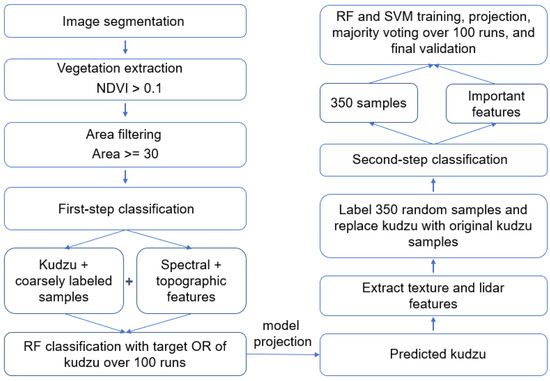
Figure 1.
Workflow of the proposed method on classifying kudzu with decreased sampling effort and computational cost.
2.3.1. Image Segmentation
Segmentation was conducted on the 4-band NAIP image taken in April 2016, as kudzu was distinctive from surrounding vegetation due to its gray color at this time of year (Figure 2). The image segmentation was conducted in ArcGIS using the mean shift segmentation function [33]. Mean shift is a powerful local homogenization technique that replaces pixel value with the mean value of pixels in a given radius (r) of neighborhood whose values vary within a given range d. Users define the r and d parameters in ArcGIS by setting the spatial and spectral detail values between 1 and 20. After visually comparing the over-segmentation and under-segmentation by different spatial detail (5, 7.5, 10, and 15) and spectral detail (5, 10, 15, and 20) values, we finally set the spatial and spectral details to 10 and 15, respectively. Quantitative metric, such as the Jaccard Index, is encouraged to use in future research to determine the spatial and spectral detail values. A scene with multiple kudzu patches from NAIP 2016 and the corresponding segmented image is shown in Figure 2.
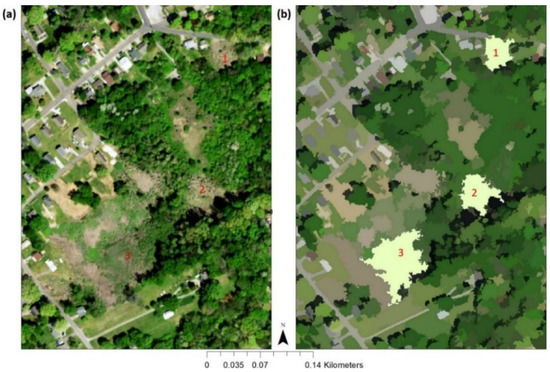
Figure 2.
(a) A scene of National Agriculture Imagery Program (NAIP) image taken in April 2016 with kudzu patches. Kudzu patch 1 and 2 represent relatively pure kudzu patches, and 3 represents kudzu patch mixed with other vegetation. (b) segments of (a) with 1, 2, and 3 correspond to the three kudzu patches in (a).
2.3.2. Vegetation Extraction and Coarsely Labeling Vegetation Objects
The normalized difference vegetation index (NDVI) derived from NAIP 2012 was used to remove non-vegetation objects, as the imagery was taken in summer (June 2012) when vegetation was most distinctive from non-vegetation. Objects with mean NDVI lower than 0.1 were classified as non-vegetation. Among the remaining vegetation, small objects with an area less than 30m2 were further excluded to decrease potential noises. NLCD 2016 was used to coarsely label all the remaining vegetation objects. The land-cover type that occupied the most area within the coverage of each vegetation object was assigned as the coarse label. Table 2 lists the percentage of each land cover class assigned as the coarse labels for all the remaining vegetation objects. The total number of vegetation objects in the study area after each preprocessing procedure is summarized in Table 3 in the Results section.
Table 2.
Percentage of each land cover class assigned as coarse labels for all the remaining vegetation objects.
Table 3.
Number of objects after each procedure and the corresponding omission rate (OR) of kudzu based on the testing and validation datasets.
2.3.3. Integration of Light Detection and Ranging (Lidar) Point Clouds
Lidar features were directly derived from the 3-D point clouds for each object (Figure 3). To derive lidar features, we first filtered out lidar points that had Z values smaller than 0 and that were out of the 95% quantile to remove potential noises for each object. We then generated a digital terrain model to subtract terrain and calculated the lidar metrics listed in Table 1. Figure 3 shows an example of the lidar point clouds for four different vegetation classes after filtering out potential noises and subtracting the digital terrain model.
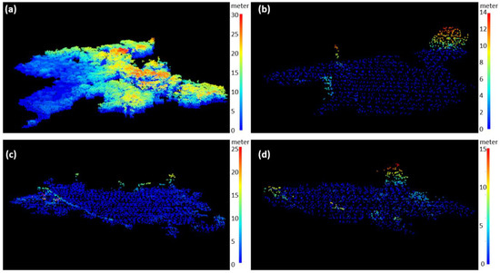
Figure 3.
Three-dimensional (3-D) lidar point clouds plot for an object of (a) forest, (b) grass, (c) kudzu, and (d) other herbaceous vegetation after filtering the potential noises and subtracting the digital terrain model. The areas of four vegetation objects in (a)–(d) are 101,902 m2, 16,033 m2, 16,034 m2, and 7430 m2, respectively.
2.3.4. Two-Step Classification
We collected 400 kudzu samples from the entire study area either by field sampling (163 samples) or visual interpretation (237 samples) using Google Earth (GE). As sample accuracy is critical for vegetation mapping, we used all images taken after year 2010 and, when applicable, zoomed into street view for confirmation when using GE to collect samples. The corresponding vegetation segments were assigned as the kudzu samples. Among the 400 samples, 20% (80) were set aside for the final validation of the model, and 80% (320) were used for the model training and testing (Figure 4a). GLCM-derived textural features and lidar point cloud-derived features were only included for the second step to decrease the computational cost.
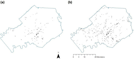
Figure 4.
(a) 320 kudzu training samples, and (b) 1010 predicted kudzu objects in Knox County by support vector machine using the proposed workflow with 3% omission rate at the first-step classification.
First-Step Classification with Coarsely Labeled Samples
Accurately labeled kudzu samples together with coarsely labeled vegetation samples were used to classify kudzu for the first step (Figure 1). RF classifier was used for the first-step classification for its high accuracy and efficiency on large datasets. All features (Table 1), except lidar point clouds and GLCM derived features, were used to construct the RF model. We randomly extracted 80% (256) of the kudzu samples from the 320 samples and a given number of coarsely labeled vegetation samples to train a RF model. The omission rate (OR) of kudzu for each RF model was evaluated using the remaining 20% (64) samples. The RF model was run 100 times, and each time a different set of kudzu training and testing samples and coarsely labeled samples were used. For the parameters of the RF algorithm, six variables were used for each split (the floored square root of the total features, 44, for the first step) and 256 trees were grown based on findings by Oshiro et al. [34].
The OR of kudzu would be impacted by the number of coarsely labeled samples used for model construction. Thus, we first determined the number of coarsely labeled samples included in each RF model to achieve target OR of kudzu over the 100 runs. We selected three testing ORs, 0.01, 0.03 and 0.05, to assess which OR at the first step could produce the best final classification accuracy of kudzu. The corresponding numbers of coarsely labeled samples for OR of 0.01, 0.03, and 0.05 were 2500, 10,000, and 20,500, respectively. However, these numbers should vary based on the type and sample size of target vegetation species, so users should determine the number of coarsely labeled samples based on their samples and expected OR. For each run, the fitted RF was used to predict the land-cover class for all vegetation objects, and the mode of the predictions over 100 runs was assigned as the predicted class.
Second-Step Classification with Accurately Labeled Samples
For the second step, 350 samples were randomly extracted from the predicted kudzu by the first step and were accurately labeled by using GE. We used randomly extracted samples to make the number of samples for each vegetation class roughly representative of actual class proportions in the remaining vegetation objects [29,30,31,35]. Among the 350 random samples, kudzu samples were replaced with the same number of samples from the original 320 training sets. The classification models were then constructed on the new 350 training data and used to re-predict vegetation objects that were classified as kudzu by the first step (Figure 1). To evaluate the commission rate (CR) of the final model, we also identified 80 non-kudzu objects (which were not included in the 350 random samples) from the predicted kudzu by the first step to be used as the validation samples. RF and support vector machine (SVM) were used in the second-step classification due to their constantly reported good performances [12,36,37]. Detailed explanations of the algorithms can be found in Breiman [38] and Cortes and Vapnik [39]. For the parameters of the RF algorithm, the number of variables randomly sampled for each split was limited to 6 (the floored square root of the selected features, details in Section 2.5 and Section 3.3), and a large number of trees, 2000, were grown to achieve good accuracy. Radial kernel was used for SVM as it yielded the best accuracy compared to all other kernels. Each model was run 100 times, and for each run a different set of kudzu samples randomly extracted from the 320 kudzu samples was used. The mode of prediction over 100 runs was taken as the final prediction for all remaining objects.
2.4. Comparison of the Proposed Method with the Traditional Method
We also employed a broadly used method, which conducts one-step sampling and includes accurate samples for all classes (hereafter traditional method), to compare its performance with the proposed workflow on classifying kudzu. The 320 kudzu samples were compiled with 800 randomly extracted and accurately labeled samples to construct the training set of the traditional method. The 800 samples included 662 forestry objects, 121 herbaceous objects (including 84 grass and 37 other herbaceous vegetation), 16 urban objects, and 1 kudzu object. As the target class was vegetation and the misclassification arose from confusion of kudzu with other vegetation classes, the small proportion of urban objects in the sample would not be a concern.
We only included lidar point cloud-derived structural features and GLCM-derived textural features in the second step of classification to decrease the computational cost. To make the traditional method comparable with the proposed method, the RF was also conducted 100 times with each run using 80% and 20% of the kudzu samples as the training and testing dataset, respectively. Similarly, the mode of prediction over 100 runs was assigned as the predicted class for all objects, and only the predicted kudzu objects were included in the second step. Given the apparent low accuracy of this method (details in Section 3.1 and Section 3.2), we also used a similar sub-sampling method for the traditional approach as follows: we randomly extracted and labeled 350 samples from the predicted kudzu by the first step and replaced kudzu with the same number of samples from the original 320 training set, and used these samples for the second-step classification.
2.5. Feature Selection, Accuracy Assessment, and Impact of Sample Size of Kudzu
Feature selection was conducted for the second-step classification for both the proposed workflow and the traditional method. For each model, we selected the minimum set of features that generated the same classification accuracy for kudzu objects as all the features for the RF model. The same minimum set of features were then used to train both RF and SVM models. Producer’s accuracy (PA, 1-OR), user’s accuracy (UA, 1-CR), and Kappa coefficient [40] were used to evaluate classification accuracy. As kudzu is the target vegetation species in this research, accuracy assessment was only conducted on the kudzu class. The 80 kudzu and non-kudzu validation samples were used to calculate the PA, UA, and Kappa. To evaluate the impact of target vegetation sample size on the classification results, we varied the number of kudzu samples used for each run of model training for the proposed method with 1% OR at the first step and for the traditional method with two-step sampling.
3. Results
3.1. First-Step Classification
Using 30 cores of a desktop computer with 128 GB RAM, the processing time on deriving lidar metrics and GLCM features for 50,000 randomly extracted objects in R program took 52 and 183 min, respectively. The first-step classification dramatically decreased the total number of objects from millions to thousands (Table 3), consequently, decreased the computational time for extracting lidar and GLCM-textural features from days to hours and reduced the computational cost by two orders of magnitude. For the proposed method, the number of predicted kudzu objects was negatively associated with the OR of kudzu class (Table 3). The OR on validation and testing data had the same values for all procedures and methods (Table 3). The OR of the traditional method was 1%, however, the number of predicted kudzu objects was higher than the proposed method with 1% OR, suggesting higher CR of the traditional method (Table 3).
3.2. Second-Step Classification
Table 4 lists the number of samples for each class among the 350 randomly extracted and accurately labeled samples. It is important to notice that the kudzu samples in the randomly extracted samples were replaced with the same number of kudzu in the training samples instead of all kudzu training samples to avoid overprediction. The sample number of each class suggested that the major misclassification of kudzu by the first step came from the confusion of kudzu with forest and herbaceous plants (Table 4).
Table 4.
Number of accurately labeled samples used for each run of model training for the second-step classification.
SVM constantly produced better accuracy than RF for the proposed method (Table 5). With 1% OR at the first step, the second-step classification had underprediction of kudzu (resulting in low PA and high UA) as a result of insufficient kudzu samples included in each run (Table 5). Both RF and SVM had higher PA but lower UA when the OR was set to 3% than 5% at the first step, and both models had the highest Kappa (0.88 for RF and 0.90 for SVM, Table 5) with 3% OR at the first step. Among all models, SVM with 3% OR at the first step had the highest classification accuracy (PA = 0.94, UA = 0.96), and 1,010 kudzu objects were predicted over the entire study area (Figure 4b, Supplementary S1).
Table 5.
Classification accuracy of kudzu on validation dataset by random forest (RF) and support vector machine (SVM) models.
Given the apparent overprediction of the traditional method and the fact that more kudzu samples included in each run led to higher overprediction (details in Section 3.3), only 50 randomly extracted kudzu samples from the 320 samples were included in each run. The traditional method with one-step sampling had overprediction of kudzu, leading to high PA but low UA (Table 5). The overprediction was a result of misclassification of grass and other herbaceous plants as kudzu (Figure 5). Using a sub-sampling from the predicted kudzu by the first step dramatically improved the classification accuracy (Table 5). However, the traditional methods had constantly lower accuracy compared to the proposed method (Table 5).
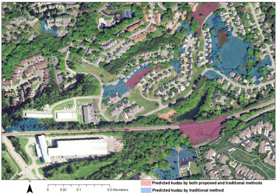
Figure 5.
A scene of detected kudzu by the best support vector machine (SVM) model using the proposed method and by the traditional method with one-step sampling using SVM. Both models detected all three kudzu patches in this landscape (shown in red), whereas the traditional method misclassified more herbaceous vegetation into kudzu (shown in blue). The image taken in April (from NAIP 2016) was used as the background image.
3.3. Feature Importance
For the second-step classification, 39, 36, and 39 features were selected and included in model construction for the proposed method with 1%, 3%, and 5% OR at the first step, respectively, and 38 features were included for the traditional method. The feature importance was determined based on ranking of SVM and RF over 100 runs with the 3% OR at the first step as it led to the best final accuracy (Figure 6). The 15 most important features ranked by both SVM and RF included 5 lidar point cloud-derived features, 5 infrared band-derived features (mostly GLCM textural features), and 5 other features (mostly NDVI features), suggesting lidar, textural, and spectral features were all important for the detection of kudzu (Figure 6). RF also ranked DEM focal change as an important feature.
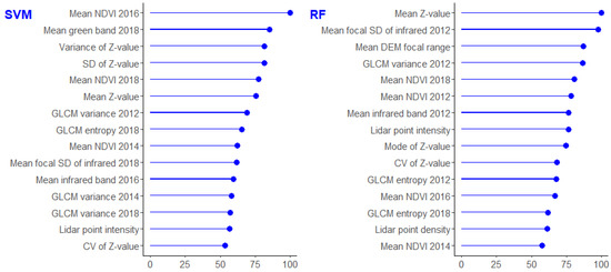
Figure 6.
The 15 most important features ranked by support vector machine (SVM) and random forest (RF) over 100 runs for the second-step classification. NDVI, SD, GLCM, and CV are acronyms for normalized difference vegetation index, standard deviation, gray-level co-occurrence matrix, and coefficient of variance, respectively. The values on x-axis indicate the importance of each variable for model construction with higher value suggesting higher importance.
3.4. Impact of Kudzu Sample Size on Classification Accuracy
Given the same set of training data for other vegetation classes, the number of kudzu samples included in each run was positively associated with the PA and the number of predicted kudzu, but negatively associated with the UA (Table 6). Interestingly, we found a quadratic relation between the number of kudzu samples included in each run and the number of kudzu predicted by both SVM and RF (R2 =1 for all models, Figure 7). Insufficient kudzu samples included in each run resulted in underprediction while too many samples led to overprediction (Table 6). Using 100 kudzu samples in each run generated the best accuracy (PA = 0.93, UA = 0.82) for the proposed method with 1% OR at the first step, whereas the traditional method failed to have good accuracy in all cases (Table 6).
Table 6.
Mean testing accuracy on classifying kudzu objects by four machine-learning models over 100 runs.
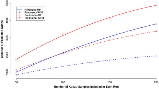
Figure 7.
Quadratic relation between the number of kudzu samples included in each run and the number of predicted kudzu objects by random forest (RF) and support vector machine (SVM) for both the proposed workflow (with 1% omission rate at the first-step classification) and the traditional method with two-step samplings. Data points represent the observed number of predicted kudzu and lines represent the fitted quadratic models.
4. Discussion
4.1. Integration of Multiple Sources of Remote-Sensing Data for Vegetation Mapping
The need for detailed vegetation mapping with reliable accuracy is increasing, and the increasing availabilities of high-resolution RS data, including multispectral and lidar data greatly facilitate this task. Integrating RS data from multiple platforms could provide a more robust set of features for better detection of target vegetation than using a single source of RS data [14,15,16], and has become an increasingly used approach for vegetation mapping at the species level [4,14,41]. Using OBIA with high-resolution RS data can mitigate the potential noises caused by within-class variation associated with high-resolution [11], as well as making it applicable to use features from both the spectral and spatial domains. Compared to the classification accuracy of kudzu achieved by Cheng et al. [27] using pixel-based hyperspectral data for a small study area (PA = 0.73, UA = 0.83), our classification on kudzu over a large spatial area produced higher accuracy (PA = 0.94, UA = 0.96). The improved performance of our method may suggest integrating high-resolution multispectral and lidar data to derive spectral, textural, and structural features could provide more robust predictors than a relatively full spectral profile for mapping some vegetation species.
4.2. Decrease of Computational Cost and Sampling Effort
Integrating multiple sources of high-resolution RS data for detailed vegetation mapping on a large spatial scale can be computationally intensive, especially for 3-D lidar point clouds data. For example, to map the tree canopy in New York City, 307 GB lidar data needed to be processed to cover the whole study area [15], and in our case 255 GB lidar data needed to be processed. Additionally, deriving GLCM-based texture features can be also computationally intensive for a large dataset. Reducing computational cost thus can facilitate vegetation mapping with high-resolution data, especially when the study area is regional or larger. Our designed workflow first generated an overprediction map of target vegetation, and dramatically decreased vegetation objects from millions to thousands for a more detailed and accurate second-step classification. Computationally intensive features, such as GLCM-derived and lidar point cloud-derived features, only need to be extracted for objects that are not distinctive from the target vegetation class for a second-step classification. In our case, this method decreased the computational time on deriving lidar and GLCM features from days to hours and reduced the computational cost by two orders of magnitude.
Combining coarsely labeled samples with accurately labeled samples has been implemented to classify extensive animal images into detailed categories [22,23] as well as to detect urban buildings [20]. Our research suggests coarsely labeled data can also facilitate the classification of vegetation at species level, and a 30 m resolution land cover product can be a good source to coarsely label vegetation samples. Using coarsely labeled samples together with accurately labeled samples of target vegetation helps to discriminate objects with distinctive features with the target vegetation species. For vegetation objects that cannot be easily distinguished from the target class, a relatively small set of accurately labeled samples, 350 in our case, extracted from the predictions by the first step can greatly refine and improve the final classification accuracy.
4.3. Sub-Sampling Improves Sample Specificity for Target Vegetation Species
We found even for the traditional method, a sub-sampling among the predicted objects from the first step greatly improved the final classification accuracy on the target vegetation species. The extreme overprediction (i.e., low UA) of kudzu using only one-step sampling should be a result that the samples failed to include sufficient vegetation samples that only occupied a small proportion in landscape but had similar features with kudzu. As a result, both RF and SVM classified these vegetation objects having similar features with target vegetation as kudzu. A sub-sampling among the predicted objects from the first step helps to optimize the sampling effort by selecting samples that are similar with target vegetation class. For vegetation mapping over a large heterogenous landscape, it could be difficult to find sufficient vegetation samples that have similar features with target vegetation. The two-step sampling method used in this research, therefore, could be conducted to improve the sampling specificity for target vegetation.
4.4. Impact of Sample Size of Target Vegetation Species
Using balanced training data with equal sample size for each class or unbalanced data with sample size of each class proportional to their area in real landscape is an unsettled concern, and both strategies have been commonly used for image classification [29,30,31,42]. Millard and Richardson [31] found that the predicted proportion of each class by RF was close to its proportion in the real landscape when the training sample size of each class resembled its real proportion in the landscape. They also found that higher proportion of each class in the training sample led to more prediction of that class by RF [31]. Our research confirmed their findings, as increasing kudzu sample size while keeping other classes unchanged increased the number of predicted kudzu. Meanwhile we found SVM also had the same pattern, and both models showed a quadratic relationship between the number of kudzu samples included in each run and the number of kudzu predicted.
Researchers found that classification tree models showed the best accuracy with unbalanced samples representing the proportion of each class in a real landscape [29,31]. Our research confirmed this finding as the best RF occurred when the number of kudzu samples in each run was determined roughly based on their proportion in all the vegetation objects. Meanwhile, SVM also showed the same pattern. However, as suggested by the underprediction of kudzu by both RF and SVM models with 1% OR at the first step, when the target vegetation species is among the minority class, using the proportion of each class rule may result in insufficient samples leading to underprediction (i.e., low PA, Table 5). On the other hand, oversampling of the minority class can lead to overprediction (i.e., low UA, Table 6) [31,42]. Consequently, the PA for the minority class could show a positive association with the number of samples included for algorithm training, whereas UA can have a negative association. Researchers suggested including a minimum number of training samples, e.g., 50, for the minority class with unbalanced samples [20]. Here we also suggest determining the optimal sampling size of the minority class used for algorithm training by balancing desired accuracy between PA and UA [43].
4.5. Use and Limitation of the Proposed Workflow
The proposed workflow could decrease computational cost as well as sampling effort for non-target classes for mapping target vegetation on large spatial scales. However, caution needs to be undertaken in the selection of OR for the first step. Higher OR at the first step leads to less computation for the second step but also leads to high OR of the final classification model. In our case, 3% OR at the first step generated the best classification accuracy in terms of PA, UA and Kappa. Although a 1% OR for the first step led to a highly overprediction of kudzu, using an appropriate kudzu sample size for training the classification algorithms at the second step still produced a good final accuracy. This finding suggests that selecting an appropriate sample size of target vegetation at the second step can overcome the overprediction by the first step. Therefore, we suggest a low OR, such as 3% and 1%, at the first step for higher final classification accuracy. Additionally, we expect our workflow to be effective for vegetation species that are separable from surroundings at a certain time of year to be segmented for OBIA. Further research will be focused on evaluating the efficiency and accuracy of the proposed workflow in mapping kudzu at a state or a national level and on detecting other vegetation species.
5. Conclusions
Integrating high-resolution multispectral image and lidar point clouds and applying OBIA can provide a robust set of features for vegetation mapping at the species level. The designed workflow using two-step classification can dramatically reduce computational cost associated with deriving computationally intensive features from high-resolution RS data over a large spatial area. Using accurately labeled samples of target vegetation and extensive coarsely labeled vegetation samples to first train an overprediction model can be an efficient method for mapping vegetation over large spatial areas to decrease sampling effort for non-target vegetation. A land cover map with 30 m resolution can be a good source to coarsely label vegetation samples. We suggest a low OR of target vegetation species at the first step to achieve good final accuracy. The workflow can also improve sampling efficiency and specificity, as a sub-sampling among the predicted objects by the first step optimizes the sampling effort by selecting samples that are not distinctive from target vegetation. Caution needs to be given to the sample size of target vegetation used to train the classification algorithm. An insufficient number of samples leads to underprediction, whereas too many samples leads to overprediction of the target vegetation. We expect the proposed workflow to be effective for vegetation classes that are separable from surroundings in order to conduct OBIA.
Supplementary Materials
The following is available online at https://www.mdpi.com/2072-4292/12/4/609/s1: Shapefile S1: 1010 predicted kudzu patch by SVM.
Author Contributions
Conceptualization, W.L., M.A., L.T., and J.G.; methodology, W.L., M.A., L.C., J.M., and Y.L.; software, W.L., L.C., and J.M.; validation, W.L.; formal analysis, W.L.; investigation, W.L.; resources, W.L. and J.G.; data curation, W.L.; writing—original draft preparation, W.L.; writing—review and editing, W.L., L.C., L.T., Y.L., and J.G.; visualization, W.L.; supervision, M.A., L.T., and J.G.; project administration, W.L. and J.G.; funding acquisition, J.G. All authors have read and agreed to the published version of the manuscript.
Funding
This research was funded by Tennessee Soybean Promotion Board.
Acknowledgments
We thank Ming Shen, Monica Papeş, Scott Stewart, and Gregory Wiggins at the University of Tennessee for valuable discussions on this research. We also thank the anonymous reviewers for their detailed and constructive comments on earlier draft of this paper.
Conflicts of Interest
The authors declare no conflict of interest.
References
- Liang, W.; Tran, L.; Wiggins, G.J.; Grant, J.F.; Stewart, S.D.; Washington-Allen, R. Determining spread rate of kudzu bug (Hemiptera: Plataspidae) and its associations with environmental factors in a heterogeneous landscape. Environ. Entomol. 2019, 48, 309–317. [Google Scholar] [CrossRef] [PubMed]
- Xie, Y.; Sha, Z.; Yu, M. Remote sensing imagery in vegetation mapping: A review. J. Plant Ecol. 2008, 1, 9–23. [Google Scholar] [CrossRef]
- Wardlow, B.; Egbert, S.; Kastens, J. Analysis of time-series MODIS 250 m vegetation index data for crop classification in the U.S. central great plains. Remote Sens. Environ. 2007, 108, 290–310. [Google Scholar] [CrossRef]
- Gilmore, M.S.; Wilson, E.H.; Barrett, N.; Civco, D.L.; Prisloe, S.; Hurd, J.D.; Chadwick, C. Integrating multi-temporal spectral and structural information to map wetland vegetation in a lower Connecticut River tidal marsh. Remote Sens. Environ. 2008, 112, 4048–4060. [Google Scholar] [CrossRef]
- Yang, J.; Weisberg, P.J.; Bristow, N.A. Landsat remote sensing approaches for monitoring long-term tree cover dynamics in semi-arid woodlands: Comparison of vegetation indices and spectral mixture analysis. Remote Sens. Environ. 2012, 119, 62–71. [Google Scholar] [CrossRef]
- Zhong, Y.; Wang, X.; Xu, Y.; Wang, S.; Jia, T.; Hu, X.; Zhao, J.; Wei, L.; Zhang, L. Mini-UAV-borne hyperspectral remote sensing: From observation and processing to applications. IEEE Geosci. Remote Sens. Mag. 2018, 6, 46–62. [Google Scholar] [CrossRef]
- Zhang, L.; Zhang, L.; Tao, D.; Huang, X. On combining multiple features for hyperspectral remote sensing image classification. IEEE Trans. Geosci. Remote Sens. 2012, 50, 879–893. [Google Scholar] [CrossRef]
- Burai, P.; Deák, B.; Valkó, O.; Tomor, T. Classification of herbaceous vegetation using airborne hyperspectral imagery. Remote Sens. 2015, 7, 2046–2066. [Google Scholar] [CrossRef]
- Alvarez-Taboada, F.; Paredes, C.; Julián-Pelaz, J. Mapping of the invasive species Hakea sericea using unmanned aerial vehicle (UAV) and WorldView-2 imagery and an object-oriented approach. Remote Sens. 2017, 9, 913. [Google Scholar] [CrossRef]
- Ahmed, O.S.; Shemrock, A.; Chabot, D.; Dillon, C.; Williams, G.; Wasson, R.; Franklin, S.E. Hierarchical land cover and vegetation classification using multispectral data acquired from an unmanned aerial vehicle. Int. J. Remote Sens. 2017, 38, 2037–2052. [Google Scholar] [CrossRef]
- Yu, Q.; Gong, P.; Clinton, N.; Biging, G.; Kelly, M.; Schirokauer, D. Object-based detailed vegetation classification with airborne high spatial resolution remote sensing imagery. Photogramm. Eng. Remote Sens. 2006, 72, 799–811. [Google Scholar] [CrossRef]
- Fu, B.; Wang, Y.; Campbell, A.; Li, Y.; Zhang, B.; Yin, S.; Xing, Z.; Jin, X. Comparison of object-based and pixel-based Random Forest algorithm for wetland vegetation mapping using high spatial resolution GF-1 and SAR data. Ecol. Indic. 2017, 73, 105–117. [Google Scholar] [CrossRef]
- Erker, T.; Wang, L.; Lorentz, L.; Stoltman, A.; Townsend, P.A. A statewide urban tree canopy mapping method. Remote Sens. Environ. 2019, 229, 148–158. [Google Scholar] [CrossRef]
- Ke, Y.; Quackenbush, L.J.; Im, J. Synergistic use of QuickBird multispectral imagery and LIDAR data for object-based forest species classification. Remote Sens. Environ. 2010, 114, 1141–1154. [Google Scholar] [CrossRef]
- MacFaden, S.W.; O’Neil-Dunne, J.P.M.; Royar, A.R.; Lu, J.W.T.; Rundle, A.G. High-resolution tree canopy mapping for New York city using LIDAR and object-based image analysis. J. Appl. Remote Sens. 2012, 6, 063567. [Google Scholar] [CrossRef]
- Suárez, J.C.; Ontiveros, C.; Smith, S.; Snape, S. Use of airborne LiDAR and aerial photography in the estimation of individual tree heights in forestry. Comput. Geosci. 2005, 31, 253–262. [Google Scholar] [CrossRef]
- Dorigo, W.; Lucieer, A.; Podobnikar, T.; Čarni, A. Mapping invasive Fallopia japonica by combined spectral, spatial, and temporal analysis of digital orthophotos. Int. J. Appl. Earth Obs. Geoinf. 2012, 19, 185–195. [Google Scholar] [CrossRef]
- Nguyen, U.; Glenn, E.P.; Dang, T.D.; Pham, L.T.H. Mapping vegetation types in semi-arid riparian regions using random forest and object-based image approach: A case study of the Colorado River ecosystem, grand canyon, Arizona. Ecol. Inform. 2019, 50, 43–50. [Google Scholar] [CrossRef]
- Narumalani, S.; Mishra, D.R.; Wilson, R.; Reece, P.; Kohler, A. Detecting and mapping four invasive species along the floodplain of North Platte River, Nebraska. Weed Technol. 2009, 23, 99–107. [Google Scholar] [CrossRef]
- Maggiori, E.; Tarabalka, Y.; Charpiat, G.; Alliez, P. Convolutional neural networks for large-scale remote-sensing image classification. IEEE Trans. Geosci. Remote Sens. 2016, 55, 645–657. [Google Scholar] [CrossRef]
- Langford, Z.; Kumar, J.; Hoffman, F.; Breen, A.; Iversen, C. Arctic vegetation mapping using unsupervised training datasets and convolutional neural networks. Remote Sens. 2019, 11, 69. [Google Scholar] [CrossRef]
- Ristin, M.; Gall, J.; Guillaumin, M.; Van Gool, L. From categories to subcategories: Large-scale image classification with partial class label refinement. In Proceedings of the IEEE International Conference on Computer Vision Pattern Recognition, Boston, MA, USA, 8–10 June 2015; pp. 231–239. [Google Scholar]
- Lei, J.; Guo, Z.; Wang, Y. Weakly supervised image classification with coarse and fine labels. In Proceedings of the 14th Conference on Computer Robot Vision, Edmonton, AB, Canada, 17–19 May 2017; pp. 240–247. [Google Scholar]
- Sun, J.-H.; Liu, Z.-D.; Britton, K.O.; Cai, P.; Orr, D.; Hough-Goldstein, J. Survey of phytophagous insects and foliar pathogens in China for a biocontrol perspective on kudzu, Pueraria montana var. lobata (Willd.) Maesen and S. Almeida (Fabaceae). Biol. Control 2006, 36, 22–31. [Google Scholar] [CrossRef][Green Version]
- Forseth, I.N.; Innis, A.F. Kudzu (Pueraria montana): History, physiology, and ecology combine to make a major ecosystem threat. Crit. Rev. Plant Sci. 2004, 23, 401–413. [Google Scholar] [CrossRef]
- Follak, S. Potential distribution and environmental threat of Pueraria lobata. Open Life Sci. 2011, 6, 457–469. [Google Scholar] [CrossRef]
- Cheng, Y.-B.; Tom, E.; Ustin, S.L. Mapping an invasive species, kudzu (Pueraria montana), using hyperspectral imagery in western Georgia. J. Appl. Remote Sens. 2007, 1, 013514. [Google Scholar] [CrossRef]
- Li, J.; Bruce, L.M.; Byrd, J.; Barnett, J. Automated detection of Pueraria montana (kudzu) through Haar analysis of hyperspectral reflectance data. In Proceedings of the IEEE International Geoscience and Remote Sensing Symposium (IGARSS), Sydney, Australia, 9–13 July 2001; Volume 5, pp. 2247–2249. [Google Scholar]
- Colditz, R.R. An evaluation of different training sample allocation schemes for discrete and continuous land cover classification using decision tree-based algorithms. Remote Sens. 2015, 7, 9655–9681. [Google Scholar] [CrossRef]
- Heydari, S.S.; Mountrakis, G. Effect of classifier selection, reference sample size, reference class distribution and scene heterogeneity in per-pixel classification accuracy using 26 Landsat sites. Remote Sens. Environ. 2018, 204, 648–658. [Google Scholar] [CrossRef]
- Millard, K.; Richardson, M. On the importance of training data sample selection in random forest image classification: A case study in peatland ecosystem mapping. Remote Sens. 2015, 7, 8489–8515. [Google Scholar] [CrossRef]
- Ball, J.E.; Anderson, D.T.; Chan, C.S. Comprehensive survey of deep learning in remote sensing: Theories, tools, and challenges for the community. J. Appl. Remote Sens. 2017, 11, 042609. [Google Scholar] [CrossRef]
- ESRI. ArcGIS Desktop and Spatial Analyst Extension: Release 10.1; Environmental Systems Research Institute: Redlands, CA, USA, 2012. [Google Scholar]
- Oshiro, T.M.; Perez, P.S.; Baranauskas, J.A. How many trees in a random forest? In Lecture Notes in Computer Science (Including Subseries Lecture Notes in Artificial Intelligence and Lecture Notes in Bioinformatics); Springer: Berlin/Heidelberg, Germany, 2012; Volume 7376, pp. 154–168. [Google Scholar]
- Ramezan, A.C.; Warner, A.T.; Maxwell, E.A. Evaluation of sampling and cross-validation tuning strategies for regional-scale machine learning classification. Remote Sens. 2019, 11, 185. [Google Scholar] [CrossRef]
- Qi, Z.; Yeh, A.G.-O.; Li, X.; Lin, Z. A novel algorithm for land use and land cover classification using RADARSAT-2 polarimetric SAR data. Remote Sens. Environ. 2012, 118, 21–39. [Google Scholar] [CrossRef]
- Feng, Q.; Liu, J.; Gong, J. UAV Remote sensing for urban vegetation mapping using random forest and texture analysis. Remote Sens. 2015, 7, 1074–1094. [Google Scholar] [CrossRef]
- Breiman, L. Random forests. Mach. Learn. 2001, 45, 5–32. [Google Scholar] [CrossRef]
- Cortes, C.; Vapnik, V. Support-vector networks. Mach. Learn. 1995, 20, 273–297. [Google Scholar] [CrossRef]
- Cohen, J. A Coefficient of agreement for nominal scales. Educ. Psychol. Meas. 1960, 20, 37–46. [Google Scholar] [CrossRef]
- Juel, A.; Groom, G.B.; Svenning, J.-C.; Ejrnæs, R. Spatial application of random forest models for fine-scale coastal vegetation classification using object based analysis of aerial orthophoto and DEM data. Int. J. Appl. Earth Obs. Geoinf. 2015, 42, 106–114. [Google Scholar] [CrossRef]
- Colditz, R.R.; Schmidt, M.; Conrad, C.; Hansen, M.C.; Dech, S. Land cover classification with coarse spatial resolution data to derive continuous and discrete maps for complex regions. Remote Sens. Environ. 2011, 115, 3264–3275. [Google Scholar] [CrossRef]
- Jin, H.; Stehman, S.V.; Mountrakis, G. Assessing the impact of training sample selection on accuracy of an urban classification: A case study in Denver, Colorado. Int. J. Remote Sens. 2014, 35, 2067–2081. [Google Scholar] [CrossRef]
© 2020 by the authors. Licensee MDPI, Basel, Switzerland. This article is an open access article distributed under the terms and conditions of the Creative Commons Attribution (CC BY) license (http://creativecommons.org/licenses/by/4.0/).