Mapping Forest Composition with Landsat Time Series: An Evaluation of Seasonal Composites and Harmonic Regression

Abstract

The Landsat program has long supported pioneering research on the recovery of forest information by remote sensing technologies for several decades, and efforts to improve the thematic resolution and accuracy of forest compositional products remains an area of continued innovation. Recent development and application of Landsat time series analysis offers unique opportunities for quantifying seasonality and trend components among different forest types for developing alternative feature sets for forest vegetation mapping. Within a large forested landscape in Southeastern Ohio, USA, we examined the use of harmonic metrics developed from time series of all available Landsat-8 observations (2013–2019) relative to seasonal image composites, including accompanying spectral components and vegetation indices. A reference dataset among three sources was integrated and used to categorize forest inventory data into seven forest type classes and gradient compositional response. Results showed that the combination of harmonic metrics and topographic variables achieved an accuracy agreement with the reference data of 74.9% relative to seasonal composites (71.6%) and spectral indices (70.3%). Differences in agreement were attributed to improved discrimination of three heterogeneous upland hardwood classes and an early-successional, young forest class, all forest types of primary interest among managers across the region. Variable importance metrics often identified the cosine and sine terms that quantify the seasonality in spectral values in the harmonic feature space, suggesting these aspects best support the characterization of forest types at greater thematic detail than seasonal compositing procedures. This study demonstrates how advanced time series metrics can improve forest type modeling and forest gradient quantifications, thus showcasing a need for continued exploration of such approaches across different forest types.

1. Introduction

The Landsat program has long supported pioneering research on the recovery of forest information by remote sensing technologies [1,2,3,4]. Efforts to improve the thematic resolution of forest compositional products, often representing heterogeneous forest types or individual species, remains an area of continued innovation [3,5,6] as such information affords insight into the dynamics, function, and resilience of ecosystems to environmental change [7,8]. Landsat data are especially valuable for several attributes, including a lengthy record of Earth surface observation, an emphasis on maintaining consistent sensor specifications through time [9], and a spatial resolution largely compatible with both local-scale management and national forest inventory programs [1,10,11]. Longstanding consensus recognizes the importance of multi-temporal images or seasonal inputs, often with accompanying spectral components or vegetation indices, which maximize spectral contrast among vegetative communities during key phenological periods [12,13,14]. The use of such data, however, is challenging, especially for large spatial extents that require reconstructing imagery across multiple Landsat orbit paths. Here, regaining spatial (related to image contamination by clouds and cloud shadows) and temporal (variation in the timing of acquisitions) continuity demands special attention.

Methodological procedures not previously available for Landsat image analysis have increased exponentially with progressive data policies beginning in 2008 that provided open access to past and future Landsat acquisitions [15]. In turn, a dramatic emergence in new research that exploits dense temporal histories of Landsat imagery have sought to reduce challenges in obtaining characteristic image values for improving vegetation mapping efforts [4,16,17,18]. Recent applications involving mathematical time series modeling, such as those based on Fourier-style and related harmonic regression techniques, have shown to reduce noise in spectral response, as well as characterize the seasonal behavior of surface observations [19,20]. These techniques have been used to define auxiliary feature sets for mapping crops [21], tropical forest types and disturbance [22], and forest types in the Midwestern and Eastern USA [23,24]. Such alternative feature sets, in the context of forest compositional modeling, have shown to improve model accuracy over more conventional single- and multi-date feature inputs and composites, while also potentially reducing bias in selecting representative values by otherwise exhaustively including all-available useful observations [23,24]. In addition, cloud-based computing platforms like Google Earth Engine (GEE) [25], have greatly reduced local computing demands and increased potential for incorporating such data into vegetation mapping efforts [24,26].

Meanwhile, the remote sensing field has also experienced experimentation into the ways in which floristic assemblages are thematically conveyed on vegetation maps. Classification, by labeling of vegetation type to map unit, has remained the predominant approach to landscape-scale vegetation mapping [1,27,28,29]. Gradient modeling has emerged as a means to reconcile conventional mapping practice with a reality that ecological communities display variation in stand transitional patterns beyond that of categorical maps [30,31,32,33,34,35,36]. Specifically, the aim of gradient modeling is the development of a non-classificatory approach that strives to represent pixels as collections of individual species without reference to any specific class membership, while preserving continuous properties of floristic change, as a result of intergrading stands of co-occurring species that gradually transition from one community to the next. Various gradient-based approaches, such as those based on canonical correspondence analysis [30] or flexible ordination-regression techniques [34,35,37], are similar concerning the transfer of detailed, plot-level species data to ordination models, in which extracted ordination values among the principal axes are utilized as response inputs to approximate compositional attributes of individual forest stands. Embodied in the overall gradient-based approach is the community-continua concept of community ecology, which combines both (i) aspects of traditional classification, and (ii) the envisioning of communities as representing collections of overlapping yet independent species distributions [35,38]. As such, unique to gradient modeling is the perceived, yet more realistic, preservation of both abrupt and grading compositional transitions expected along environmental and ecological pathways as individual species respond to one another and the conditions that define species-specific resource needs [31,39].

The potential values added from these new capabilities of Landsat data, and the tools to model with them, led us to develop an approach for modeling both forest type and gradient response in an established study area in Southeastern Ohio, USA. Our study area spans four Landsat scenes and features a diverse array of tree species, making it an ideal candidate space for this study. Our primary objective was to compare the effectiveness of alternative spectral metrics with more conventional seasonal inputs and composites derived from all available Landsat-8 data coincident with a diverse reference dataset. Specifically, we tested the utility of harmonic metrics comprising modeled coefficients extracted from time series modeling of spectral components and vegetation indices with seasonal spectral inputs developed from compositing procedures. Our primary goal was to develop the metrics to better understand the contributions of individual features and determine how these advanced procedures perform in an applied forest management setting. In order to evaluate the contribution of these advanced approaches, we evaluate if harmonic features improve the discrimination of forest types, particularly those of most concern to management, including the accurate representation of oak-dominated (Quercus spp.) and early-successional forest types, represented in discrete classes and continuous ordination values in the reference dataset. We, therefore, have a basis to ensure that outputs from these tools represent well the environmental conditions existing on the ground such that they can be applied to forest management planning at a landscape scale.

2. Materials and Methods

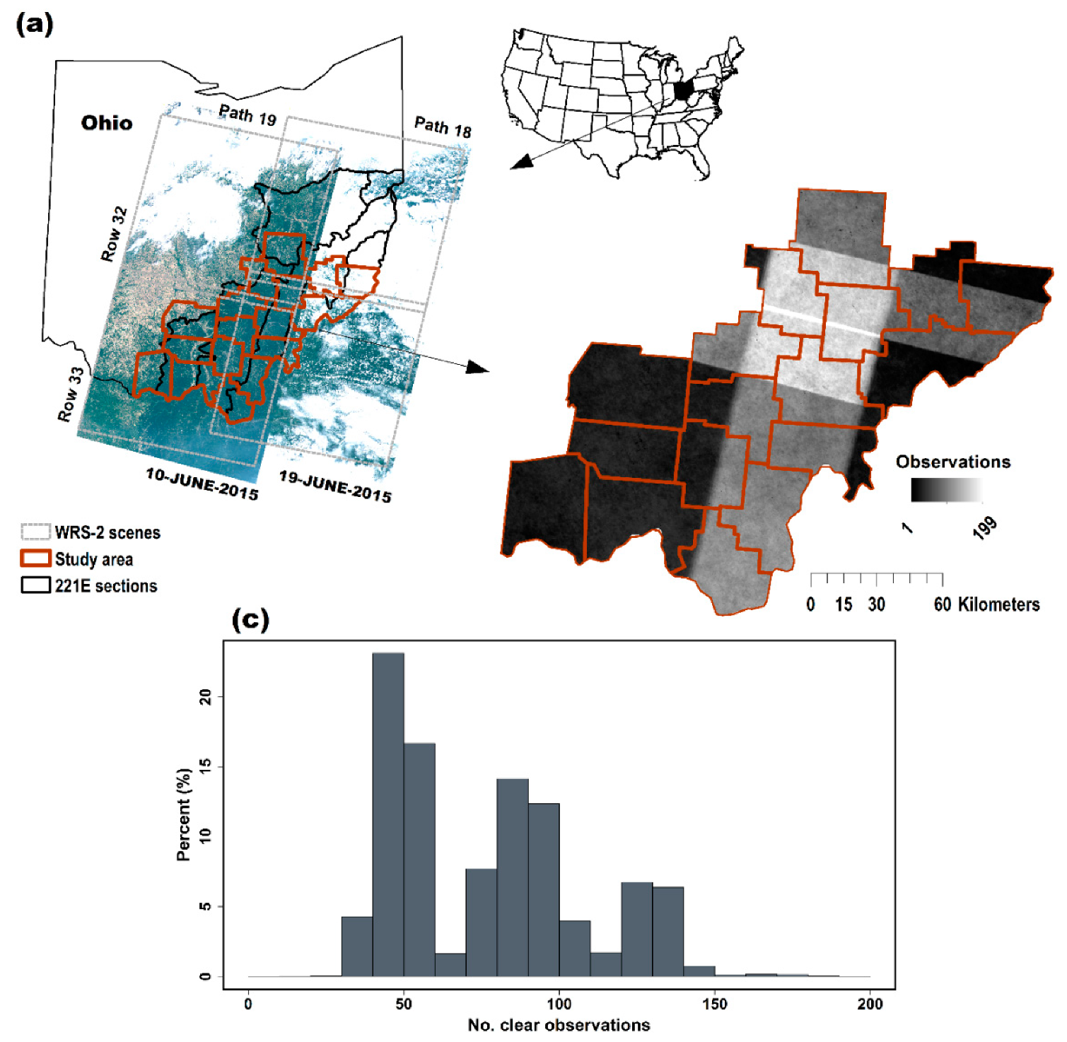
2.1. Study Area

The study area was selected to intersect with an area previously established as part of a Collaborative Oak Management Project through the USDA Joint Chief’s Restoration Partnership [40,41]. Here, 17 counties (encompassing four WRS-2 scenes (Path/Row), 18/32, 18/33, 19/32, and 19/33) within the Ohio portion of the Southern Unglaciated Allegheny Plateau Section (221E) [42] were identified for these efforts (Figure 1). The area has been the focus for targeted and coordinated management by the Ohio Interagency Forestry Team and a project to document current status and trends for each of the five subsections and 15 ecological landtypes (ELT) [40,41]. This large area is located primarily just south of the Maximum Wisconsin Glaciation and features an unglaciated and highly dissected terrain with relatively low relief. Floristic assemblages closely track the topographic contours of the study area, and a system based on the ecological landtypes has long been established for ecological classification of forest types in the study area [40,43]. Specifically, dry-oak assemblages (Quercus spp.) typically dominate the dry ridgetops and southwestern hillslopes and transition to mixed-mesophytic assemblages on opposing northeastern hillslopes and bottomlands. The landscape is predominately forested at ~69% and dominated by a speciose hardwood community including 77 tree species [41]. Major species include Quercus alba, Q. rubra, Q. montana, Q. velutina, Acer rubrum, A. saccharum, and Liriodendron tulipifera. Native conifers, notably Pinus virginiana, Pinus rigida, and Tsuga canadensis, appear interspersed at relatively low densities with native hardwoods, and several monospecific plantations of a few species, such as Pinus echinata and P. strobus, are planted throughout the study area. Like much of the eastern US, the predominant forest cover is the result of heavy exploitation - specifically, here, beginning during the period 1850–1900, to provide charcoal for a short-lived iron industry [44]. Subsequently, in the absence of fire, the oak-dominated forests (Quercus spp.) have been transitioning to more mesic species, predominately maples (Acer spp.) [45,46].

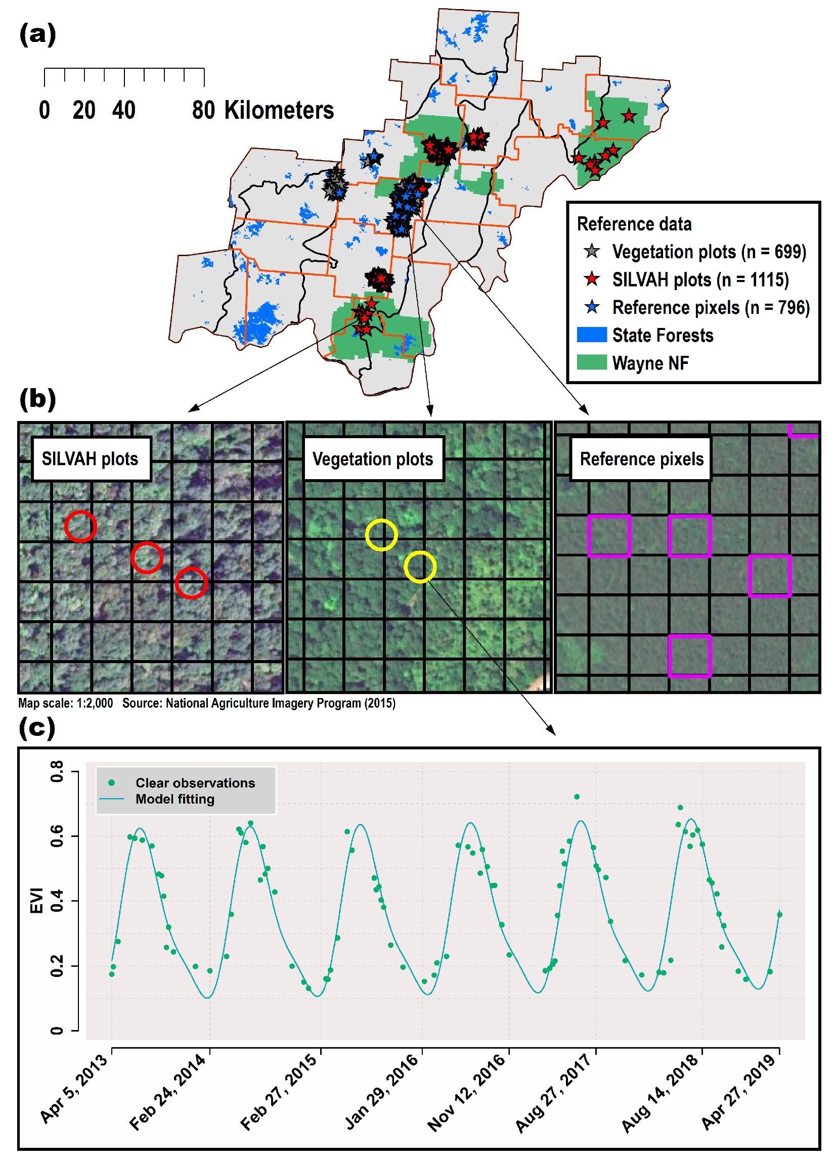
2.2. Forest Reference Data

Reference data coincident with the operational lifespan of Landsat-8 were acquired from three sources and among several state forests, parks, wildlife management areas, and the Wayne National Forest across the study area (Figure 2). Information provided among the three datasets varied according to compositional detail (e.g., overstory and understory forest inventories versus pre-labeled reference pixels) and were leveraged individually or in combination according to the objectives of either compositional modeling task: classification of forest types or gradient modeling of ordination values. The first dataset included forest inventories collected using standard Silviculture of Allegheny Hardwoods (hereafter SILVAH plots) [47] protocol (n = 1115 plots) as part of the ongoing Ohio Interagency Forestry Team’s emphasis for the study area. The SILVAH dataset utilized a plot-less methodology in which 10- or 20-factor prisms were used to identify trees (i.e., overstory stems) located at each point. These point estimates provide dominate species coverage for specific locations across the study area. Relevant measurements that followed included species identification and a diameter at breast height (DBH) recording taken on each “in” tree [48]. Only records with trees of ≥8 cm DBH were used in further analysis from the SILVAH dataset. The second dataset included a dense vegetation inventory (hereafter vegetation plots; n = 699 plots) collected using a fixed-radius (11.3 m; ~400 m²) protocol, established following a spatially-stratified cluster sampling design among several forest units in the center of the study area [34]. Trees and other live stems ≥8 cm DBH were identified and DBH recorded within each plot. An additional nested subplot (5-m radius; ~100 m²) was established within each full plot to collect data on understory woody stems <8 cm DBH and ≥1 m in height (i.e., shrubs and advance regeneration). All live woody stems were identified to species in both datasets, with a few exceptions in the following genera: Carya, Crataegus, Salix, Smilax, Vaccinium, and Vitis. For consistency, genus was used for these species only. Finally, because these inventories demonstrated a bias towards upland mature hardwood stands, a third dataset including reference pixels (n = 796; hereafter reference pixels) of bottomland floodplains, pine-dominated stands, and early-successional (i.e., recent clear-cuts) young forests and shrublands was acquired to bolster the overall reference dataset [29]. These data were developed through ground-truthing and orthophoto interpretation. Further details on the reference data are provided in each compositional modeling approach.

2.3. Digital Data Acquisition and Processing

Multispectral image data were queried and processed within the GEE online browser interface. We used all available Landsat 8-Operational Land Imager (OLI) images with <80% cloud coverage inclusive from 5 April 2013 to 27 April 2019 among the four WRS-2 scenes of the study area, totaling 330 images. The images were all Level-2 (USGS Landsat Science Products) Surface Reflectance data, including the latest generation orthorectification, radiometric calibration, and atmospheric correction protocol (LaSRC) [49]. Clouds and cloud shadows were masked using the CFmask [50] pixel_qa band included in each image before analysis (Figure 1 displays the spatial distribution of the number of clear observations across the study area after masking). All subsequent clear observations from the reflectance data were arranged into a dense time series, and coefficients provided by [51] were used to append Tasseled Cap Transformation (TCT) component bands to each image, including Tasseled Cap Brightness (TCB), Tasseled Cap Greenness (TCG), and Tasseled Cap Wetness (TCW). In addition, the enhanced vegetation index (EVI) was also calculated for each image (

Table 1. Variables, brief descriptions, and abbreviations of the four feature sets used in forest compositional modeling.

Landsat 8-OLI (P 18-19/R 32-33; 330 Images)		Date Range (Years)/Abbv.
Seasonal composites (Bands 1–7)
	Leaf-on (Summer)	1 June–30 August (2014–2017)
	Transition (Fall)	15 September–15 November (2014–2017)
	Leaf-off (Winter)	1 December–28 February (2014–2018)
	Transition (Spring)	1 April–1 May (2014–2017)
Seasonal TCT/Spectral indices composites [51]
	Tasseled Cap Brightness	TCB
	Tasseled Cap Greenness	TCG
	Tasseled Cap Wetness	TCW
	Enhanced Vegetation Index	EVI
Harmonic metrics (2nd order Fourier series coefficients)
	Mean (intercept)	INT
	Trend (slope)	TRE
	Cosine terms 1-2	CO1, CO2
	Sine terms 1-2	SI1, SI2
	RMSE	RMS
Topographic variables
	DEM: Elevation (30 m)	ELE
	Slope [52]	SLO
	Transformed aspect: Eastingness [53]	EAS
	Transformed aspect: Northingness [53]	NOR
	Topographic Wetness Index [54]	TWI
	Topographic Position Index [55]	TPI
	Deviation from mean elevation [55]	DEV

).

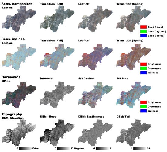
2.3.1. Composite Images

Median value composites of each Landsat multispectral band and spectral index (TCT and EVI) were calculated for the four Northern Hemisphere temperate seasons, including leaf-on (i.e., summer; June–August), leaf-off (i.e., winter; November-February), and two transition periods (i.e., fall [September–November]; and spring (April–May)) from the time series (see Table 1 for specific dates). We selected median values over concern for residual cloud or snow contamination that potentially remained following initial processing. Because cloud contamination made it impossible to develop seamless coverage for each season in a given year, the composites utilized observations across four years (2014–2018) of observation for each seasonal composite in the time series collection. The final seasonal composites defined two multi-band feature sets; one including, for each of the four seasons, the individual multispectral bands (bands 1–7; n = 28 bands; hereafter seasonal composites) and another including the three TCT components + EVI feature space for each season (n = 16; hereafter spectral indices composites).

2.3.2. Time Series Modeling

We used ordinary least squares (OLS) regression in GEE to fit Fourier-style harmonic regression equations including a trend term to each pixel and spectral component and EVI across the entire time series collection:

$${\rho }_i={\beta }_0+{\beta }_1{x}_t+{{\displaystyle \sum }}_{j\in N}\left[{\beta }_{2j}cos\left(\frac{2\pi j}{T}{x}_t\right)+{\beta }_{2j}sin\left(\frac{2\pi j}{T}{x}_t\right)\right]+{\mathsf{\epsilon }}_t,$$

(1)

where N is the order of harmonics and ε_t the residual error term for each observation. We converted Landsat image timestamps, which are stored in milliseconds since the start of the epoch (1 January 1970), to fractional days over this timeframe (x_t). The length of the annual cycle, T, equaled 365.2421891 ephemeris days per tropical year. Finally, the overall (intercept) and long-term trend (slope) coefficients are specified by β₀ and β₁x_t, respectively. The function of the trend term relates to capturing potentially important information related to variation in vegetation response to climate variability, growth, or land management that may be useful in discriminating forest types [20]. The resulting coefficients obtained from each pixel’s time series as well as the root mean square error (RMSE) described the mean annual reflectance, trend, and seasonality (i.e., cosine and sine terms) of image values. Harmonic models were fit to only the TCT + EVI bands [24].

Landsat time series developed across multiple scenes include zones of overlap along neighboring paths (i.e., sidelap) and rows (i.e., endlap), which can produce differences in the density of image values available for model fitting. In particular, this could lead to spatial artifacts in the resulting harmonic images if not carefully considered. In balancing competing demands for deriving a representative sample of harmonic metrics (given variation in the number of observations across the study area) and obtaining enough useful variables in the feature set, we tested regression models with one to four harmonics (i.e., 1st to 4th order Fourier series) to determine the model structure that best produced generalizable results across the entire region. To do this, we built models for each of the one to four orders and carefully inspected RGB composites of intercept, cosine, and sine terms and RMSE of the TCT components for the identification of spatial discontinuities in the harmonic regression output, particularly at zones of overlap. We settled on a final model form that included a 2nd order Fourier series (i.e., six total terms) as higher order models produced visually inconsistent regression results at scene boundaries [24]. Finally, coefficients, as well as the RMSE of residual error, estimated from the time series models were exported as separate seven-band images for each of the TCT + EVI indices, which included the intercept, slope, each cosine and sine terms, and RMSE. An example time series model fitted to EVI is displayed for a selected pixel in Figure 2, portraying the framework for the inputs used among the harmonic metric feature space.

2.3.3. Environmental Variables

Forest compositional modeling has been shown to be dramatically improved in our study area with the incorporation of ancillary datasets joined with multispectral imagery [34]. Therefore, we obtained a 10-m digital elevation model (DEM) derived from USGS 7.5 minute quadrangle contours from the Ohio Environmental Agency Division of Emergency and Remedial Response. From the DEM, we derived (i) elevation (m; DEM), (ii) slope (°; SLO) [52], transformed aspects, (iii) eastingness (EAS), and (iv) northingness (NOR), characterizing the north and east orientation of slopes [53], (v) topographic wetness index (TWI) [54], (vi) topographic position index (TPI) [55], and (vii) topographic deviation (DEV) [55] variables to develop an ancillary topographic feature space for forest compositional modeling.

2.4. Data Analysis

The individual feature sets (i.e., seasonal composites and harmonics metrics) developed in GEE were downloaded locally and extracted for the reference data. Specifically, plot-wise values from each feature set were sampled according to an area-weighted mean of pixel values (as reference plots were not typically centered on pixels and may include more than one pixel) intersecting a 30-m resolution square window (native Landsat resolution) centered on each reference sample location (Figure 2 displays the proximity and spatial relationship between the sampling grains of the three reference datasets and individual Landsat pixels). This window size was carefully selected as an adequate solution for stabilizing coherence in spatial attributes (i.e., sampling grain), Landsat image resolution, and geolocational precision, among the imagery and reference data at the finest grain size possible [34]. While coarsening the sampling grain, including multi-pixel kernels, has been shown to improve model accuracy in other applications [56], we were largely constrained by rapid transitions in species composition indicative of the dissected topography of the region (e.g., many ridges are <30 m wide). Thus, we found that including a sampling grain that matched the size of a single Landsat pixel best satisfied our motivations for representation of fine-scale vegetation patterns, while accommodating the sampling area of a reference plot with additional room for locational imprecision. Finally, we were confident, based on reported GPS errors (<8 m), that spatial uncertainty in field reconnaissance was similar to that of the geometric precision in the Landsat data, which has been shown to most dramatically influence results relative to sampling grain in Landsat-based applications [57].

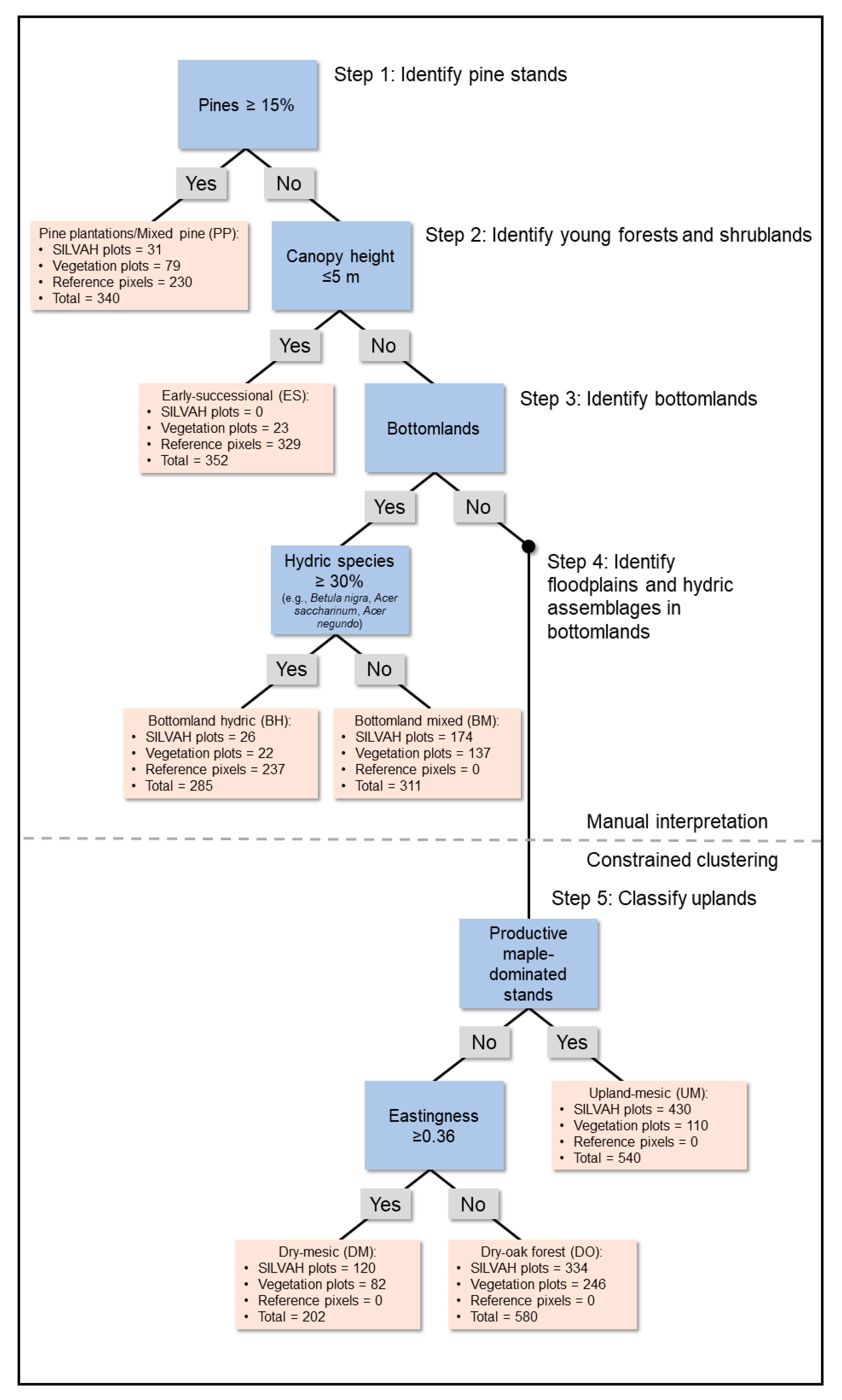
2.4.1. Forest-Type Grouping

Since the reference plot data were acquired in raw inventory form, we developed a flexible classification system to categorize the plot data into forest type classes to enable modeling of pixel-level estimates of forest types across the study area. Our hierarchical approach combined (i) manual interpretation of the detailed plot data with (ii) data-driven constrained clustering of a subset of plots. As previously described, slope orientation and location in context to ridgetops and bottomlands, is the predominant natural mechanism for compositional turnover in the study area [40,43]. Thus, our classification system incorporated this perspective into a landtype/central taxonomic tendency and/or physiognomic concept. To prepare the two inventories (detailed vegetation and SILVAH plots) for classification, local stem densities (stems ha^–1) and basal areas (m² ha^–1) were computed for each tree species/genera, and final compositional variation was expressed by calculating an importance value (IV) for each taxon for each plot [46,58]. The IVs were calculated by summing the relative density and relative basal area of each species/genera per plot. In each dataset, only records pertaining to large stems (i.e., trees) ≥8 cm DBH were used in developing our system. The IVs were used to identify canopy dominance, as well as indicator species scores [59]. After merging the two inventories, a total of 68 woody plant species/genera were considered for plot-level grouping in our classification. A decision tree summarizing our decision rules is provided in Figure 3.

The initial steps in our manual interpretation included isolating and classifying reference plots among pine plantations and mixed-pine stands (PP); recent timber harvests (ES; i.e., early-successional young forest and shrublands); and floodplains (BF) and mixed hardwood stands in bottomlands (BM). The remaining upland plots were subjected to a constrained clustering, specifically a multivariate regression tree (MRT) analysis [60]. We chose MRT over more conventional unconstrained approaches because it allowed the assisted clustering of the detailed plot data into groups defined by the aforementioned topographic variables already utilized in our manual interpretation. We found this approach to also produce the most sensible plot groupings over unconstrained approaches. The MRT procedure operates similarly to a univariate decision tree. A Euclidean distance matrix was approximated for the original species-by-plot matrix in which each explanatory variable was used to partition the plots into separate groupings that best minimized the within-group sums of squared error. The most parsimonious tree was then determined through cross-validation by repeating the procedure over several iterations, each time withholding 1/3 of the data for validation. The ancillary topographic and seasonal spectral indices data were used as explanatory variables. The use of topography in assisting the forest type grouping is particularly important in reflecting longstanding research and management practices on different site conditions determined by topography in the study area [40,45]. The best solution identified three forest types that included dry-mixed mesophytic (DM), upland mesophytic (UM), and dry-oak dominated (DO) stands. The MRT analysis was performed in the R statistical environment (https://cran.r-project.org/) with functions provided in the mvpart package [61]. Following grouping, we apportioned community labels, descriptions, and diagnostic species to each forest type, provided in

Table 2. Forest type classes developed from the reference inventory datasets.

Class Name	Abbv.	Diagnostic Species	Sample Size
Early-successional	ES	…	352
Pine plantations/Mixed pine	PP	Cercis canadensis, Pinus resinosa, Pinus rigida, Pinus strobus, Populus grandidentata	340
Floodplain hardwoods/Bottomlands hydric	BH	Aesculus flava, Betula nigra, Fraxinus americana, Juglans nigra, Platanus occidentalis, Ulmus americana	285
Bottomlands mixed hardwoods	BM	Fagus grandifolia, Liriodendron tulipifera	311
Dry-mesic mixed mesophytic hardwoods	DM	Carya spp.	202
Upland mesophytic hardwoods	UM	Acer saccharum, Tilia americana, Quercus rubra	540
Dry-oak dominated hardwoods	DO	Quercus alba, Quercus coccinea, Quercus montana, Quercus velutina	580

. Diagnostic species were based on species scores from an indicator species analysis, which incorporated the product of the relative frequency and abundance of each species in each class, proposed by Dufrêne and Legendre (1997). To augment sample sizes in poorly represented classes in the reference inventory data, the aforementioned additional dataset including 796 reference pixels of the PP, BH, and ES classes, selected from ground-truthing and orthophoto interpretation, was also incorporated [29], bringing the total sample size of the reference classification dataset to 2610 pixel-level estimates of forest type for image classification.

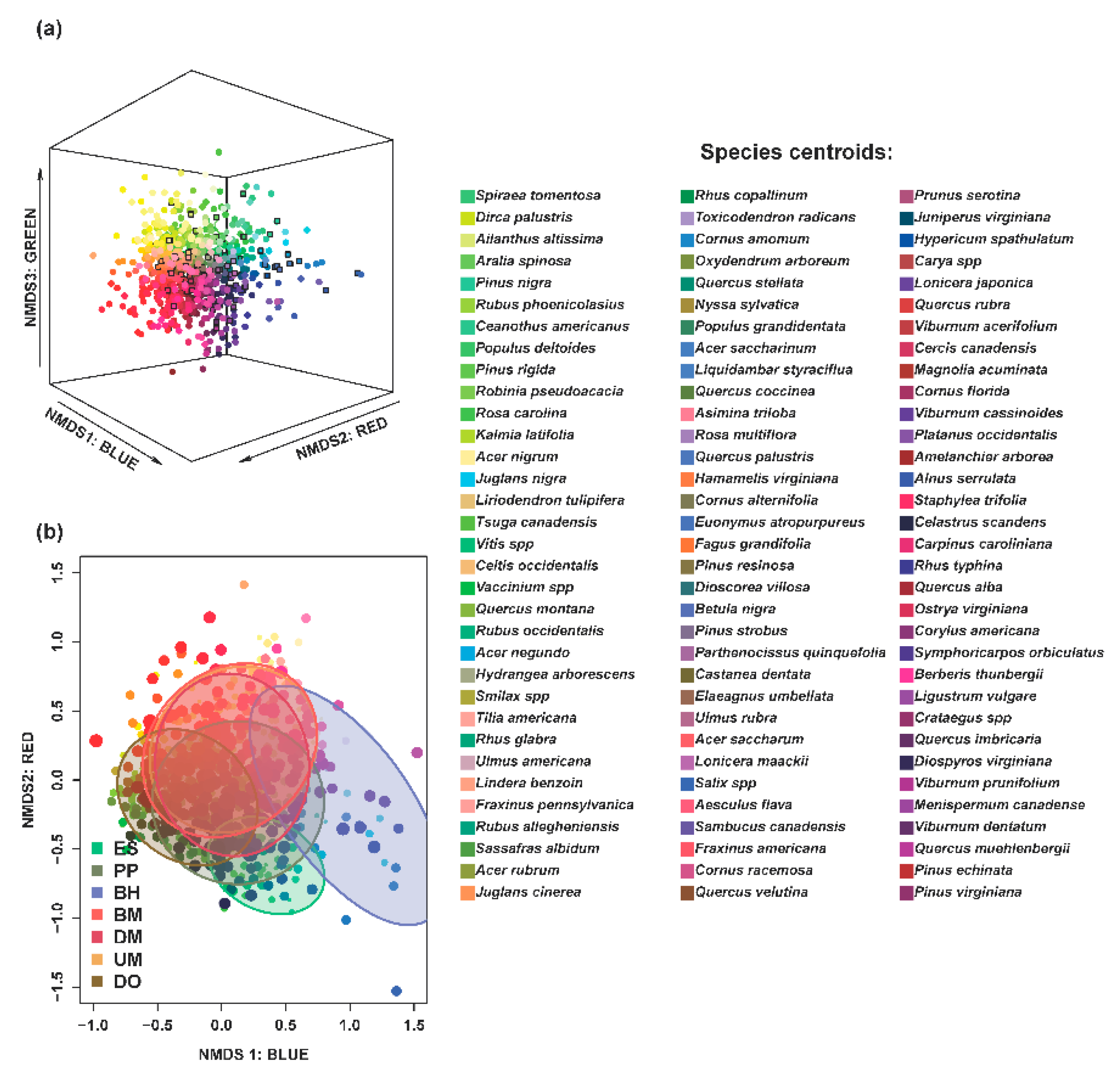
2.4.2. Compositional Ordination

We used an ordination-regression approach for gradient modeling of forest composition across the study area [34,35,37]. The goal of ordination is the reduction of complex ecological datasets to a smaller number of dimensions that preserve the underlying compositional gradients among a reference sample. The resulting ordination scores were then modeled across the study area to relate mapped locations with similarity to the original dataset in the gradient modeling approach. Non-metric multidimensional scaling (NMDS) was chosen for its non-parametric nature and flexibility in accommodating user-specified distance matrices and desired number of dimensions (k). The dense vegetation plot data, including stem counts from both overstory and understory species, were selected as the reference data for this approach. Local stem densities (stems ha^-1) from both the small and large stem data and basal areas (m² ha^-1) of large stems among 99 woody plant taxa were used to generate IV for each species/genus among each plot. Functions provided in the vegan package [62] in R were used to ordinate the species dataset onto a three-dimensional, k = 3, solution. Bray–Curtis dissimilarity was selected for the distance matrix due to its handling of "null" values (i.e., zero species abundances) among pairs of sample plots. The ordination procedure was initiated following Wisconsin and square root transformations [62]. The NMDS procedure uses an interactive approach to sample entity placement in the final gradient space. It begins with an initial random arrangement, then reorders the data striving to maximize the rank-order correlation between the original compositional distances and the distances in the reduced space. The minimum "stress" solution, i.e., maximally correlated with the original distances among those solutions tried, was subjected to a principal component rotation to achieve an expression of maximum floristic variation among the three orthogonal axes. A maximum of 500 random starts was employed, and the final solution was obtained following a minimum stress value being achieved twice in a row. The specific dimensionality was chosen such that each of the axes could be assigned to one of each of the three channels in the RGB color space [31].

2.4.3. Compositional Modeling

Random Forest (RF) was selected for relating forest type and gradient response to the various features due to both categorical and continuous responses in the study. The RF algorithm is particularly suited to ecological and remote sensing applications for its non-parametric nature, ability to handle large numbers of predictors while remaining largely immune to overfitting, and convenient internal mechanisms for assessing model agreement and identifying useful predictor variables [63,64,65]. Reference classifications were made on the field plot groupings based on the frequency of classifications by individual trees, in which the most frequent (i.e., mode) class was assigned to each plot, while continuous ordination scores utilized the mean response across all decision trees. For both compositional modeling tasks, we held all specifications to the default values, except tuning the number of trees to 1001 for each response and feature set. We chose to use an odd number of trees to prevent ties for classifications based on the mode. For continuous models of NMDS ordination axes scores 1-3, individual RF models were tuned for each axis, including three models for each feature set and combination. Functions provided in the randomForest package in R were used for RF classification and regression (supporting data is found in Supplementary Materials: Data).

2.5. Agreement Assessment

Though RF includes pseudo-independent internal validation procedures, by aggregating predictions of individual decision trees across out-of-bag (OOB) test samples, we included an additional agreement assessment to approximate more traditional procedures and to generate confidence intervals around mean/median agreement scores [23,35]. We employed a 30 × three-fold cross-validation approach, in which the reference data were partitioned into three folds with each fold being withheld for evaluation over 30 iterations. Model predictions were made onto each fold, then averaged across all folds within each iteration, and finally across all iterations. Fold assignment was held constant to ensure that each feature set was evaluated on the same testing data each time [23]. We report both the OOB and cross-validated (CV) agreement scores. We also include mean confusion matrices to examine class-level agreement differences between each feature set and combination. Confusion matrices were quantified as the mean number of correctly and incorrectly labeled samples of withheld folds in the CV agreement assessment. This involved RF predictions onto the withheld datasets, each with 870 reference samples. Mean confusion matrices report user’s and producer’s agreement scores of the CV reference labeling. Finally, we used the pseudo-R² and RMSE to evaluate model accuracy of the feature sets on continuous ordination scores of the gradient modeling approach. The modeling approach provides a statistical indicator of the relative importance of individual features towards supporting detailed forest compositional modeling in the region.

2.6. Feature Importance Assessment

A feature importance assessment was conducted to determine the utility of individual inputs among the top-performing feature set for discerning categorical and gradient responses of forest composition. Although identifying the importance of individual features can be performed in many ways with RF, we chose permutation of importance, which tracks increases in error on permuting specific predictors during OOB predictions. This procedure was done internally by the RF routine by comparing the original predictions to another set of predictions in which variables are randomly reshuffled and the difference in prediction error is averaged across all trees. Increases in error taken as the percentage decrease in mean accuracy and mean square error for categorical and continuous responses, respectively, from permuted features onto OOB predictions determined feature importance scores. Large increases in error were taken as a sign for the utility of a given feature. Mean feature importance values were pooled across OOB predictions over the 30 iterations of the OOB agreement assessment. Importance values for individual features were also computed at the class-level of individual forest types.

2.7. Mapping Output

The top-performing RF classification and regression models were trained on the full reference datasets to generate maps of discrete forest types and gradient compositional distribution across the study area. We include categorical forest type and class probabilities for classification responses. Models depicting predicted axes scores were transferred to RGB color space. By expressing the three-dimensional ordination space position in terms of variation in color, floristic gradient maps provide a visual aid for tracking similarity of mapped locations to the original reference plot data. Species scores in the original NMDS solution provide meaningful context for approximating stand-level assemblage composition across the study area. A forest mask utilizing the latest (2016) National Land Cover Database and each forest-type class (including shrub/scrub and woody wetlands) was used to avoid interpretation over spatially irrelevant areas (i.e., non-forest) in the study area [66]. Note that our accuracy assessment based on agreement with the reference data does not follow standard mapping practices according to validation against independent data. Therefore, our agreement assessment should reflect only a statistical indicator of the relative performance of individual feature sets and caution is encouraged when interpreting maps of the top-performing RF classification and regression models.

3. Results

3.1. Compositional Attributes

The NMDS analysis on the dense vegetation plot inventory converged after 123 iterations, resulting in a stress metric of 19.1 and a total of 77.2% of the floristic variation in Bray–Curtis dissimilarities being transferred to the final solution (Figure 4). This comprised 37.5%, 27.2%, and 12.5% of the variation being assigned to axes 1–3, respectively. Plot coordinates were mapped according to channels of color in RGB color space, with axes 2, 3, and 1 being applied to the red, green, and blue channels, respectively (Figure 4). This color combination was chosen as the best for maximizing visual contrast among colors (i.e., pixel-level estimates of forest composition) on the final map. The first, second, and third axes were determined to be related to moisture and ELT, successional state, and the underlying bedrock and topography across the study area, respectively [34]. Ellipses are displayed on the ordination to visualize relative compositional similarity of the forest types developed in our classification relative to gradient compositional turnover (Figure 4).

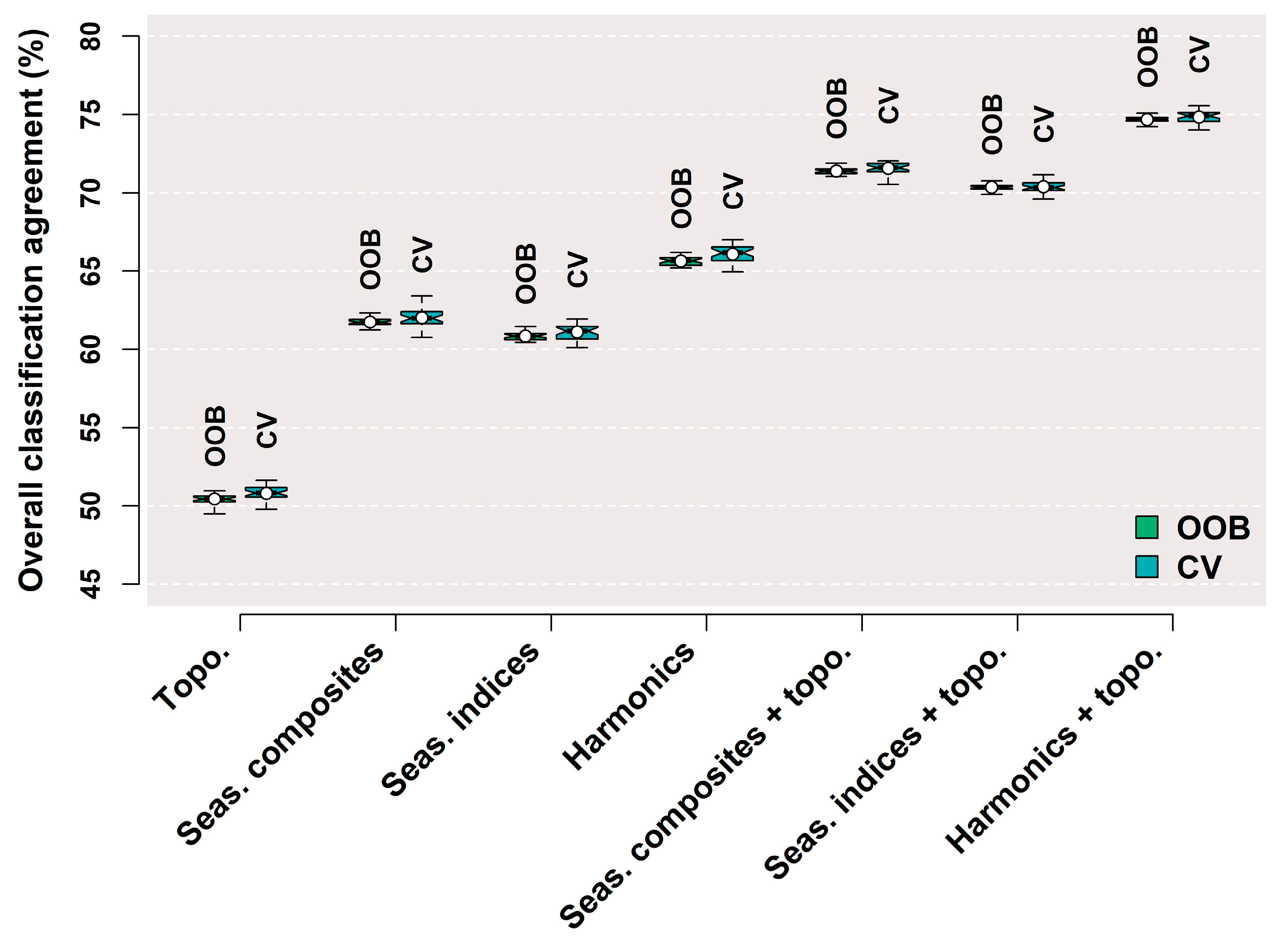
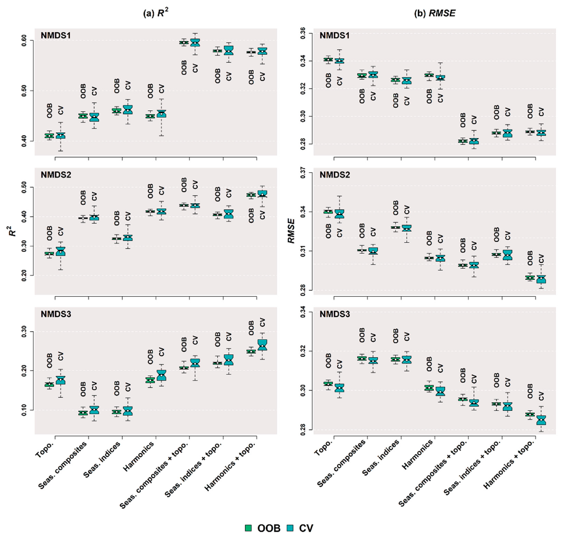
3.2. Feature Set Agreement

Overall classification accuracy (%) determined by OOB and cross-validated (CV) agreement scores did not vary significantly by approach—though the OOB agreement displays less range in variability (Figure 5). Therefore, we will only discuss CV agreement scores in detail for the following. Variation did emerge, however, as a function of the feature set used for classification. The topographic feature set exhibited the poorest accuracy overall at 50.84 ± 0.18% (median ± 95% C.I.). Considering the spectral and harmonic feature sets alone, harmonics outperformed seasonal composites composed of multispectral bands 1–7 and spectral indices (TCT + EVI) and included non-overlapping confidence intervals: 66.19 ± 0.25% versus 61.99 ± 0.22% and 61.17 ± 0.23%, respectively. As expected, the best results were achieved when combining the spectral and ancillary topographic feature sets. For these sets of models, the combination of harmonics and topography exhibited the best agreement between the reference dataset and RF results: 74.92 ± 0.17% versus 71.61 ± 0.15% and 70.34 ± 0.14%, for composite and spectral indices feature set combinations, respectively.

For the RF results of continuous NMDS ordination scores, results were less decisive, with CV scores quite similar among the datasets for three possible reasons. First, although OOB and CV scores of accuracy and error in terms of R² and RMSE were also similar among the feature sets, CV assessments demonstrated a greater range in variability as might be expected for this agreement approach (Figure 6). Second, a trend towards decreasing accuracy with each subsequent dimension in the ordination largely reflected the total volume of floristic information transferred to each subordinate axis as part of the NMDS procedure of rotating the best solution to orthogonal gradients of maximum floristic variation. Finally, the variation in agreement between feature sets and combinations largely reflected the orthogonal nature of the different ecological gradients among each axis and the strength of each feature set and pairing in capturing this information.

For the first axis, representing a moisture and ELT gradient, individual feature sets and combinations of spectral, harmonic, and topographic features formed two distinct groups in the assessment, with the latter combinations achieving the best results. These feature sets exhibited CV R² scores of 0.60 ± 0.004, 0.58 ± 0.005, and 0.58 ± 0.004 for seasonal composites, spectral indices, and harmonics, including topographic features, respectively. The second gradient, representing successional state and stand structure, exhibited CV R² scores of 0.44 ± 0.004, 0.41 ± 0.009, and 0.47 ± 0.006 for seasonal composites, spectral indices, and harmonics, including topographic features, respectively. Assessments for the third axis, which included additional topographic discrimination of forest composition, included CV R² scores of 0.22 ± 0.006, 0.23 ± 0.008, and 0.26 ± 0.008 for seasonal composites, spectral indices, and harmonics, including topographic features, respectively. An increase in accuracy is also observed for the topographic feature set alone, reflecting the related terrain gradient on this axis: 0.16 ± 0.005.

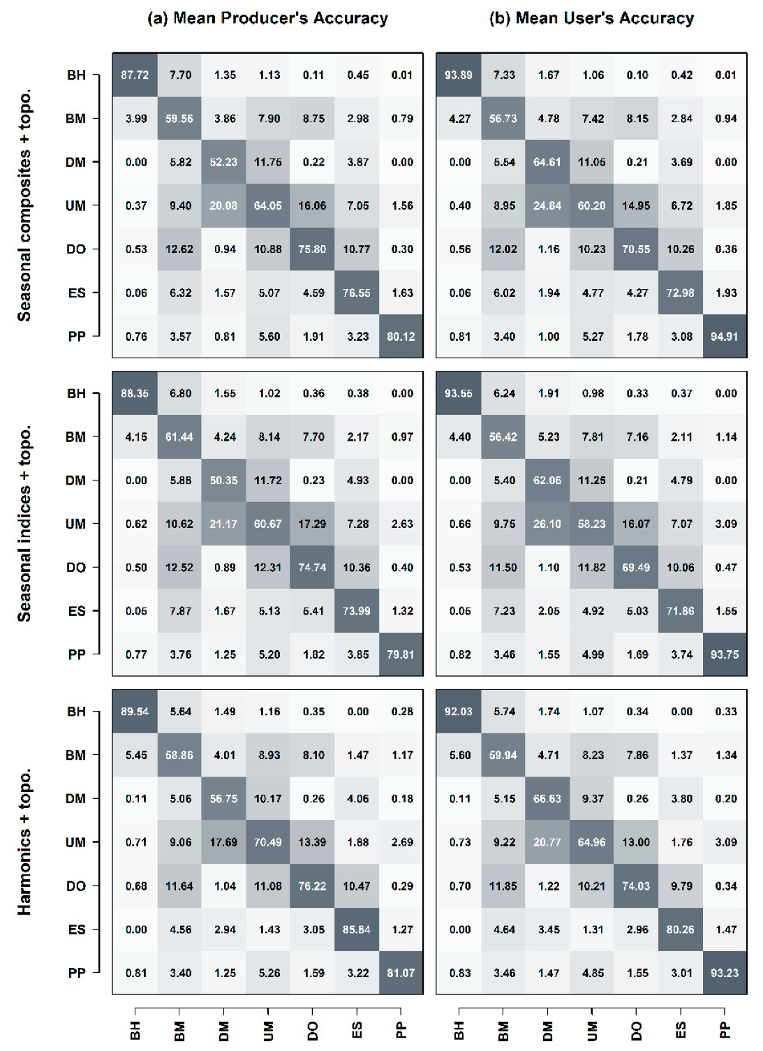
3.3. Forest Type Agreement

Confusion matrices of the mean number of correctly and incorrectly labeled reference samples as part of the CV agreement assessment demonstrate nuanced subtleties in the top-performing feature set pairings for discerning individual forest types. Taken together with confusion matrices of producer’s and user’s agreement (Figure 7), it is revealed that taxonomically distinct (such as the pine plantations/mixed pine, PP, and dry-oak dominated, DO, classes) and ecologically specialized (such as floodplains/bottomland hydric, BH) classes are modelled effectively by the spectral and topographic pairings. Confusion did emerge for the discrimination of upland hardwood classes DM, UM, and DO, which despite differences in diagnostic species, dominance, and landtype occurrence, likely exhibit considerable overlap in co-occurring species and thus spectral response. However, confusion between these classes is dramatically reduced with harmonic inputs. The greatest difference between seasonal composites/indices and harmonic metrics is observed for the early-successional (ES) class. Mean producer’s and user’s accuracy are increased by 9.29%–11.85% and 7.28%–8.40% with harmonic metrics relative to seasonal composites for this class. These results provide encouraging evidence that metrics capitalizing on full-temporal histories of Landsat surface observations in quantifying spectral trend and seasonality support discrimination of forest types at greater detail than compositing procedures.

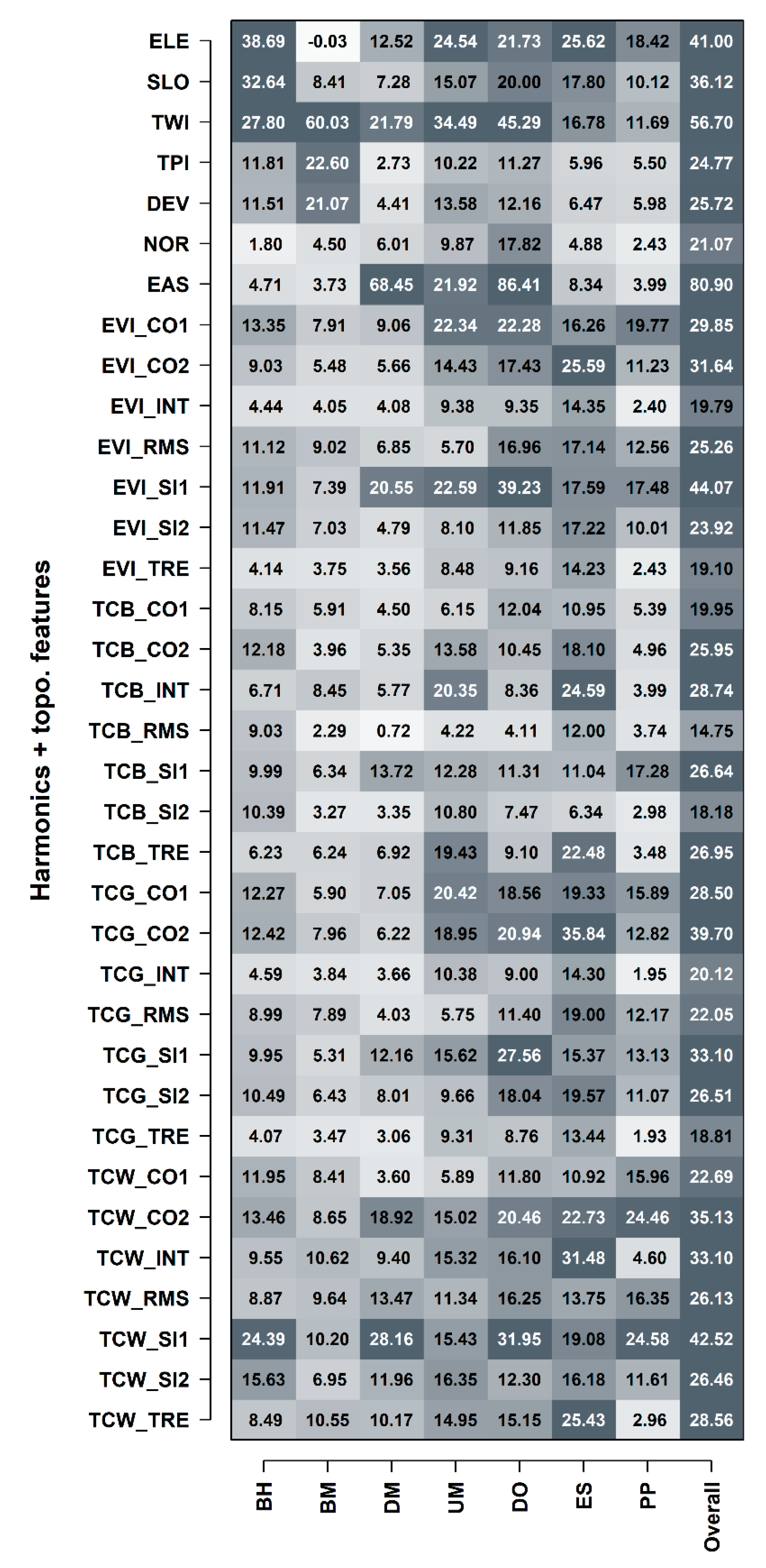
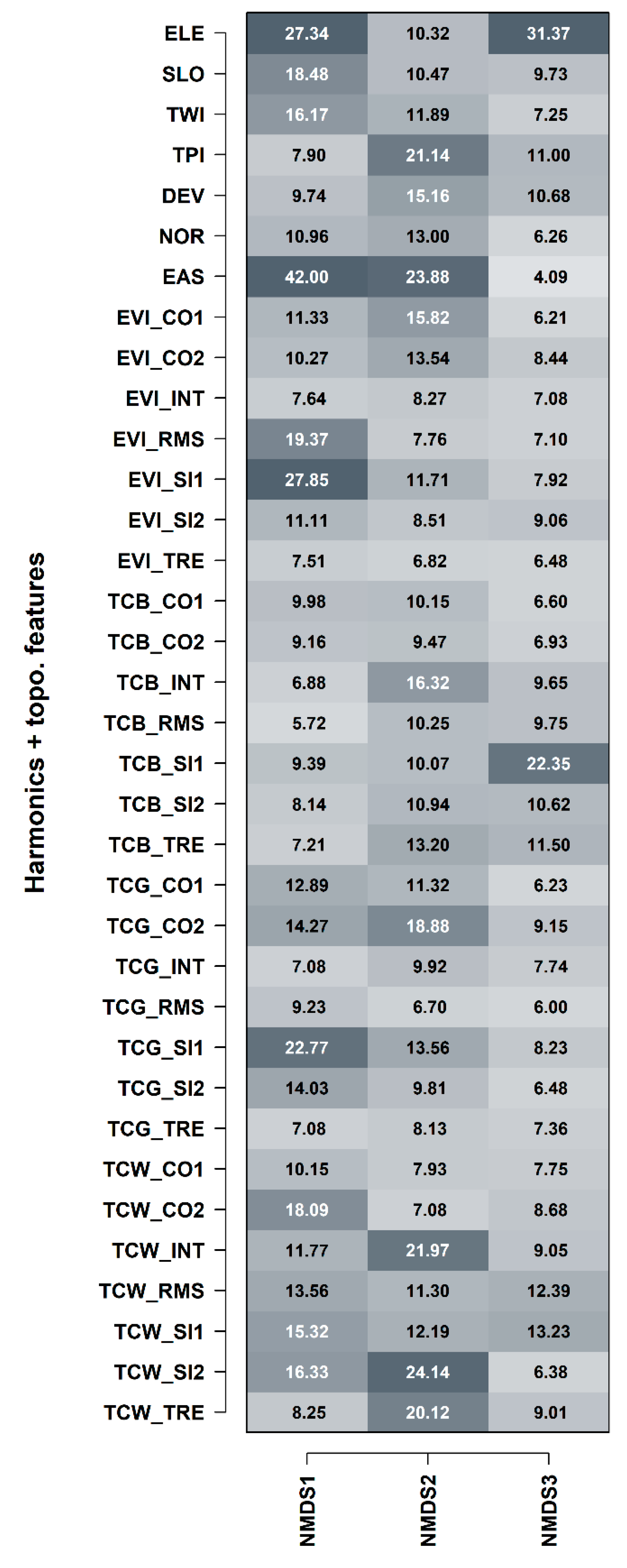
3.4. Feature Importance

Feature importance values for RF classification of forest types showed high importance of topographic variables in the top-performing harmonic and topographic pairing for both overall accuracy and accuracy at the class-level, as might be expected given the importance of this dimension in driving ecological separation of forest types in the study area and our classification system (Figure 8). Important topographic variables included transformed aspect, eastingness, and TWI. Among harmonic features, cosine and sine coefficients, describing the seasonality in TCT components and EVI, periodically emerged as top predictors at both the overall and class-level. Shared across multiple classes was the importance for these terms fitted specifically to TCW. Feature importance’s for RF regression models of NMDS ordination axes scores generally mirrored that of categorical classification of forest type (Figure 9), with transformed aspects and elevation (ELE) being particularly important. Important harmonic features included the sine terms fitted to EVI, TCW, and TCB.

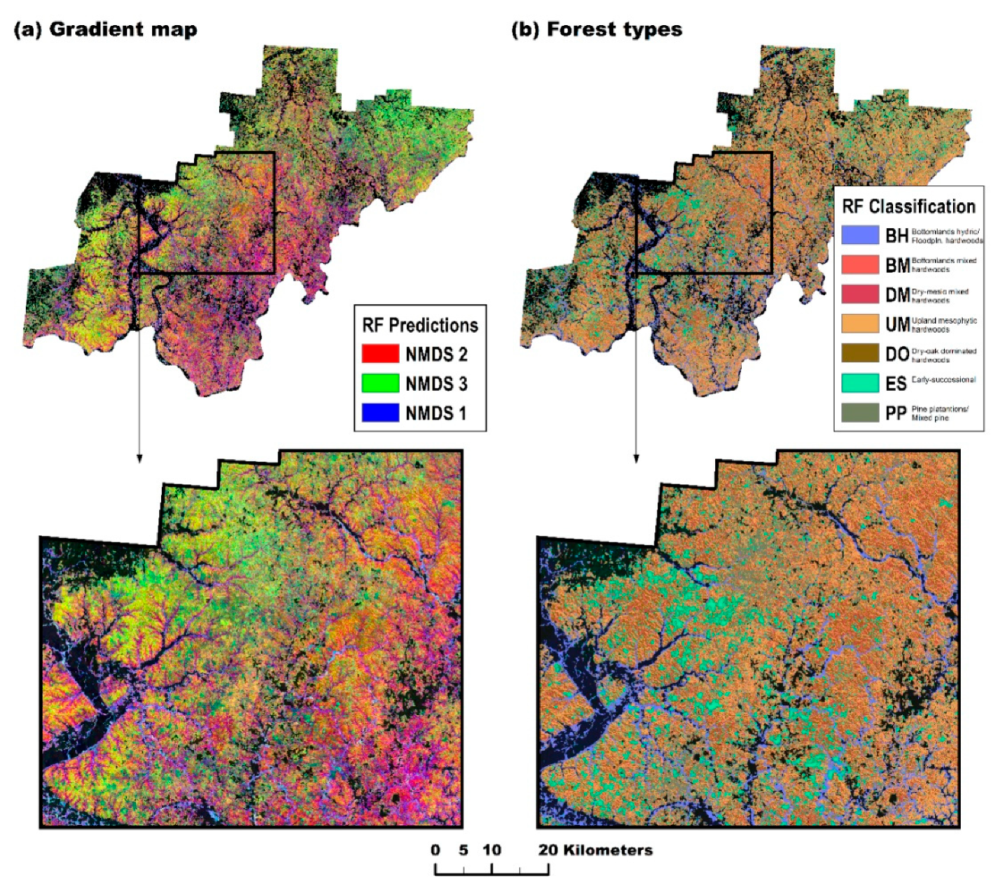
3.5. Compositional Maps

The RF classification and regression models were applied to the harmonic and topographic pairing for deriving maps of categorical and gradient forest composition across the study area (Figure 10). Color is used as a visual aid for referencing three-dimensional ordination space position with context to the reference field data on the gradient map. Color charts of species scores within the solution provide a means for approximating a species composition of individual stands across the study area (Figure 4). Categorical versus gradient compositional maps reflect differences in ecological interpretation. While categorical maps display a typical forest type and dominant taxonomy, the gradient approach highlights natural gradation, as well as abrupt breaks, between stands of co-occurring species, without reference to any specific class membership. At broad scales, maps of discrete forest types show an overall preponderance of mesophytic forest assemblages across the study area in both upland and bottomland positions. Tracking the steep venation and stream channels is the bottomland hardwood (BH) class. Dry-oak dominated stands (DO) appear in particularly rugged landscapes in the center of the study area. A finer spatial scale of interpretation shows the dominance of these assemblages on dry ridgetops and southwest facing slopes, matching the dry oak landtype of Iverson et al. (2019, 2018).

Continuous ordination scores reflected on the gradient map provide a more intricate picture of this thematic detail. For example, the preponderance of green hues among oak forests in the western portion of the study area contrast with that of the red hues in the east, reflecting a transition in Quercus montana to Q. alba/velutina dominance moving west to east across the study area. Floodplains/bottomland hydric (BH) assemblages appear as light blue hues, reflecting high NMDS1 values allocated to the blue channel. Mesophytic assemblages of BM and UM classes appearing in various pink hues on the gradient map reflect varying quantities of Ostrya virginiana, Fraxinus americana, Acer saccharum, Aesculus flava, Fagus grandifolia, and Quercus rubra occurrence in these forests. This gradient perspective supports the natural transition between bottomland and upland mesic forests. Though these maps require independent validation, they provide support for the relative performance of harmonic features. In addition, they provide baseline coverage of forest types that can be used in targeting new sampling locations and validation efforts.

4. Discussion

We developed models of discrete forest types and gradient compositional response across a large 17-county forested landscape, including four Landsat WRS-2 scenes, in Southeastern Ohio. Rather than focusing on a single or a small number of images over time, the development of technical approaches for extracting information from dense times series of satellite imagery has emerged as a consequence of improved access and processing capabilities with Landsat data. The advantage of these new approaches is the accommodation of all-clear observations available for a region of interest down to the pixel-level. While mathematical time series modeling has enhanced capability for in-filling missing data [19,20] and disturbance change detection [67], such quantification of patterns in the seasonal behavior of spectral reflectance are also beginning to provide improved characterization of forest communities at broad spatial extents [23,24]. The feasibility and application of such approach requires examination across different forest types. We found that harmonic metrics improved classification of seven forest types in our study area over compositing procedures. While the results of the gradient response were not as distinct, we did observe marginal improvements for differentiating among 699 reference samples in subordinate axes, particularly the second and third axes.

4.1. Forest Type Classification

Overall classification accuracy of the seven forest types improved ~3%–5% (from 70.3%/71.6% to 74.9%), including non-overlapping confidence intervals, with the use of feature set pairings coupling harmonic metrics with topography in comparison to the seasonal composites and spectral indices pairings. Importantly, harmonic metrics improved characterization of the primary forest cover. Specifically, confusion matrices of producer’s and user’s agreement, examining disagreement at the class-level, revealed improved discrimination of the dry-mesophytic (DM), upland mesophytic (UM), dry-oak (DO), and early-successional (ES) forest types based on harmonic metric pairings relative to seasonal composites. Accurate maps of these forest types are considered highly important to our study area and ongoing efforts, both for improving our understanding of the local forest ecology of the region and for regional land management and restoration [40]. Mesophication of oak-dominated forests to predominantly maple species assemblages remains a pernicious challenge for the study area and region at large [45,68,69]. In addition, combining forest management with the conservation of imperiled young forest conditions [70] is also considered an important prospect for the conservation of shrubland-dependent wildlife communities in the Eastern US [71]. For these reasons, the use of mathematical time-series modeling provides an effective platform for large-extent forest classification where detailed maps of these forest types are required to assist localized management of forest resources.

Inspection of harmonic metric importance values revealed relatively high rankings of the cosine and sine terms in our evaluation, lending additional support for mathematical time-series modeling of Landsat imagery for improving forest vegetation mapping. These terms describe the seasonality in spectral response as part of the annual phenological cycle among different vegetative communities. All of the spectral components and indices were selected among the top features as well, indicating that all of the TCT feature space was important to forest type classification. The seasonal behavior in the TCW component (particularly the first sine term) was especially important to bottomland floodplain (BF) classification, as expected for this forest class defined by its floodplain habitat. Interestingly, our inclusion of a trend term, describing inter-annual variation, was important in early-successional (ES) class accuracy, corresponding to the expectation for an increasing trend in brightness and greenness, and interestingly, trends in wetness as stands develop closed canopies and recover from disturbance [20]. As such, inter-annual variation should be considered when using time-series modeling metrics with classification systems that incorporate early-successional forest types. The RMSE term, describing the fit of the harmonic-style model to individual pixels, did exhibit high rankings among overall and pine plantations/mixed pine (PP) classification accuracy, suggesting this approach is also appropriate for identifying coniferous forest types among hardwood assemblages. In such case, this term provided a physical basis for discriminating between highly-seasonal deciduous and rather aseasonal coniferous forest types.

4.2. Gradient Modeling

Gradient modeling, the depiction of continuous compositional turnover resolved in ordinations of detailed plot-level species data, has emerged as a means to improve or complement the characterization of vegetation composition represented on categorical vegetation maps [34,35,72]. Ordination values mapped across regions of interest and merged into multi-band color images provide a visual cue to multidimensional ordination space position and the approximation of assemblage composition with respect to the original field data without referring to any specific class membership. Our evaluation revealed that these results were less decisive among the various feature set inputs in comparison to the classification models. In part, differences in agreement reflect the nature in compositional expression between classification versus continuous responses in these disparate approaches. However, differences in agreement between ordination gradients regressed against spectral properties among the various feature sets observed here are not entirely reconcilable. For example, we found that incorporating harmonic metrics improved explained variance (R²) among NMDS axes two (from 44% to 47%) and three (from 22% to 26%) relative to seasonal composites. Gradient modeling by nature is subject to the constraints imposed by individual species ordering along presumed underlying causal pathways and the contributions of each gradient towards explaining the total floristic volume. As such, each preceding axis is presumed to correspond to increasingly subsidiary gradients, both ecologically and environmentally, in terms of assemblage composition and their drivers, in which plot differentiation becomes less pronounced and characterized by more compositional subtleties with extension to greater dimensionality. Improved differentiation in reference data among subordinate axes thus corresponds closely to the interpretation of forest type classification that time-series metrics can provide important information necessary for characterizing vegetative communities with increased thematic detail.

Particularly important time-series metrics among the harmonic and topography feature space also included cosine and sine terms fitted to the spectral components and vegetation indices time series. This was especially true for the first axis, describing a topographic and ELT gradient among the forest compositions in the reference data. For this axis, the first sine term fitted to EVI emerged as particularly important. Trend coefficients, interestingly, supported improved accuracy among reference data along the second axis, describing a successional and structural gradient, mirroring findings for the early-successional (ES) class among the classification models. Models of the third axis, representing the most challenging axis to model in our study for the reasons previously described, on average identified the first sine term fitted to TCB as particularly important. Though explaining the least amount of the total floristic volume, accurate modeling of this dimension is particularly important for expressing the gradual transition in dominant oak species across the study area.

4.3. Time Series Processing, Applications, and Future Directions

Of course, not trivial to our evaluation and its application to forest types and gradient analysis are the various processing steps and decisions required for extracting spectral properties from dense satellite time-series data. While multi-seasonal images and, by extension, compositing procedures designed to approximate single-date acquisitions over large extents [10,73] have been utilized for some time, key limitations remain. For example, the timing of key phenological events, such as peak fall color or spring green-up, can vary dramatically over different years for the same forest type [23,74,75], further complicating the effectiveness of image composites. These comparisons provide a critical perspective into the effectiveness of time-series metrics for modeling forest types and composition, particularly for heterogeneous forest types. Specifically, in our case, the relatively short six-year window of Landsat 8 data provides a synoptic and broadly reproducible platform that overcomes some of the processing decisions and uncertainties required when using dense satellite time-series data. Furthermore, harmonized Landsat 8 and Sentinel-2 data show great promise in increasing the information content available for future time series analysis [76].

Combining traditional classification and gradient modeling approaches for expression of forest types and compositional turnover across this heterogeneous study area is expected to support numerous end users. An immediate application concerns the ongoing forest plan revision for the Wayne National Forest. Questions related to transitions occurring in oak-dominated forests, along with their regeneration potential, are paramount in their planning. In this case, combining the land types mapped for the region [40,41] with the forest type classes and species-level maps presented here provides new detailed information for planning and management. From there, further analyses can occur under multiple scenarios of future management decisions in a changing climate. For example, climate-related risks and opportunities, by species or forest type, could be spatially evaluated [77]. In addition, the models presented here could be used in targeting new sampling efforts or validation sites in improving future model outcomes with harmonic time series modeling. The near future is bright for providing new, robust, and detailed information on forests, their ecology, and their management, with the advent of time-series modeling of Landsat data coupled with powerful analytical tools available to all.

5. Conclusions

Satellite remote sensing of forest resources has long been a crucial tool for bridging the interface between strategic forest management and spatial analyses. In this study, we present results that bolster the use of time-series metrics for improving forest type modeling, in addition to perspectives on the use of such tools. Agreement with the reference data improved the classification of forest types using harmonic metrics, as compared to seasonal composites. Accuracy gains were most noticeable for discerning among three heterogeneous upland hardwood classes (i.e., dry-mesophytic, DM; upland mesophytic, UM; and dry-oak, DO) and the early-successional class (ES), each of which are of primary interest to forest managers across the region. In addition, models of gradient response trended towards improved discrimination of the reference data among subordinate axes—a powerful result, considering the importance of gradient modeling for future avenues of work in the study area and elsewhere. The results here should provide a meaningful comparison and augment our current understanding of the effectiveness of times-series modeling for improved forest type mapping [78]. The harmonic feature space used here also provides other key advantages over the long-term standard of compositing procedures, especially overcoming the challenges of selecting representative image values corresponding to important phenological events necessary for accurate forest discrimination by satellite data. The use of mathematical time series modeling as a source of direct metrics remains an exciting frontier for forest compositional modeling—not possible without the free- and open-access to Landsat data—and continued work should be pursued.

References

1. Wulder, M.A.; Coops, N.C.; Roy, D.P.; White, J.C.; Hermosilla, T. Land cover 2.0. Int. J. Remote Sens. 2018, 39, 4254–4284. [Google Scholar] [CrossRef] [Green Version]
2. Cohen, W.B.; Goward, S.N. Landsat’s role in ecological applications of remote sensing. Bioscience 2006, 54, 535–545. [Google Scholar] [CrossRef]
3. Iverson, L.R.; Graham, R.L.; Cook, E.A. Applications of satellite remote sensing to forested ecosystems. Landsc. Ecol. 1989, 3, 131–143. [Google Scholar] [CrossRef]
4. Wulder, M.A.; Masek, J.G.; Cohen, W.B.; Loveland, T.R.; Woodcock, C.E. Opening the archive: How free data has enabled the science and monitoring promise of Landsat. Remote Sens. Environ. 2012, 122, 2–10. [Google Scholar] [CrossRef]
5. He, H.S.; Mladenoff, D.J.; Radeloff, V.C.; Crow, T.R. Integration of GIS data and classified satellite imagery for regional forest assessment. Ecol. Appl. 1998, 8, 1072–1083. [Google Scholar] [CrossRef]
6. Kerr, J.T.; Ostrovsky, M. From space to species: Ecological applications for remote sensing. Trends Ecol. Evol. 2003, 18, 299–305. [Google Scholar] [CrossRef]
7. Perera, A.H.; Peterson, U.; Pastur, G.M.; Iverson, L.R. Ecosystem Services from Forest Landscapes: Broadscale Considerations; Springer: Cham, Switzerland, 2018; pp. 1–265. [Google Scholar]
8. Tilman, D.; Knops, J.; Wedin, D.; Reich, P.; Ritchie, M.; Siemann, E. The influence of functional diversity and composition on ecosystem processes. Science 1997, 277, 1300–1302. [Google Scholar] [CrossRef] [Green Version]
9. Roy, D.P.; Wulder, M.A.; Loveland, T.R.; Woodcock, C.E.; Allen, R.G.; Anderson, M.C.; Helder, D.; Irons, J.R.; Johnson, D.M.; Kennedy, R.; et al. Landsat-8: Science and product vision for terrestrial global change research. Remote Sens. Environ. 2014, 145, 154–172. [Google Scholar] [CrossRef] [Green Version]
10. White, J.C.; Wulder, M.A.; Hobart, G.W.; Luther, J.E.; Hermosilla, T.; Griffiths, P.; Coops, N.C.; Hall, R.J.; Hostert, P.; Dyk, A.; et al. Pixel-based image compositing for large-area dense time series applications and science. Can. J. Remote Sens. 2014, 40, 192–212. [Google Scholar] [CrossRef] [Green Version]
11. McRoberts, R.E.; Cohen, W.B.; Erik, N.; Stehman, S.V.; Tomppo, E.O. Using remotely sensed data to construct and assess forest attribute maps and related spatial products. Scand. J. For. Res. 2010, 25, 340–367. [Google Scholar] [CrossRef]
12. Dymond, C.C.; Mladenoff, D.J.; Radeloff, V.C. Phenological differences in Tasseled Cap indices improve deciduous forest classification. Remote Sens. Environ. 2002, 80, 460–472. [Google Scholar] [CrossRef]
13. Wolter, P.T.; Mladenoff, D.J.; Host, G.E.; Crow, T.R. Improved forest classification in the northern Lake States using multi-temporal Landsat imagery. Photogramm. Eng. Remote Sens. 1995, 61, 1129–1143. [Google Scholar]
14. Zhu, X.; Liu, D. Accurate mapping of forest types using dense seasonal landsat time-series. ISPRS J. Photogramm. Remote Sens. 2014, 96, 1–11. [Google Scholar] [CrossRef]
15. Woodcock, C.E.; Allen, R.; Anderson, M.; Belward, A.; Bindschadler, R.; Cohen, W.; Gao, F.; Goward, S.N.; Helder, D.; Helmer, E.; et al. Free access to Landsat Imagery. Science 2008, 320, 1011. [Google Scholar] [CrossRef] [PubMed]
16. Kennedy, R.E.; Andréfouët, S.; Cohen, W.B.; Gómez, C.; Griffiths, P.; Hais, M.; Healey, S.P.; Helmer, E.H.; Hostert, P.; Lyons, M.B.; et al. Bringing an ecological view of change to Landsat-based remote sensing. Front. Ecol. Environ. 2014, 12, 339–346. [Google Scholar] [CrossRef]
17. Pasquarella, V.J.; Holden, C.E.; Kaufman, L.; Woodcock, C.E. From imagery to ecology: Leveraging time series of all available Landsat observations to map and monitor ecosystem state and dynamics. Remote Sens. Ecol. Conserv. 2016, 2, 152–170. [Google Scholar] [CrossRef]
18. Banskota, A.; Kayastha, N.; Falkowski, M.J.; Wulder, M.A.; Froese, R.E.; White, J.C. Forest monitoring using Landsat time series data: A review. Can. J. Remote Sens. 2014, 40, 362–384. [Google Scholar] [CrossRef]
19. Brooks, E.B.; Thomas, V.A.; Wynne, R.H.; Coulston, J.W. Fitting the multitemporal curve: A fourier series approach to the missing data problem in remote sensing analysis. IEEE Trans. Geosci. Remote Sens. 2012, 50, 3340–3353. [Google Scholar] [CrossRef] [Green Version]
20. Zhu, Z.; Woodcock, C.E.; Holden, C.; Yang, Z. Generating synthetic Landsat images based on all available Landsat data: Predicting Landsat surface reflectance at any given time. Remote Sens. Environ. 2015, 162, 67–83. [Google Scholar] [CrossRef]
21. Wang, S.; Azzari, G.; Lobell, D.B. Crop type mapping without field-level labels: Random forest transfer and unsupervised clustering techniques. Remote Sens. Environ. 2019, 222, 303–317. [Google Scholar] [CrossRef]
22. Shimizu, K.; Ota, T.; Mizoue, N. Detecting forest changes using dense Landsat 8 and Sentinel-1 time series data in tropical seasonal forests. Remote Sens. 2019, 11, 1899. [Google Scholar] [CrossRef] [Green Version]
23. Pasquarella, V.J.; Holden, C.E.; Woodcock, C.E. Improved mapping of forest type using spectral-temporal Landsat features. Remote Sens. Environ. 2018, 210, 193–207. [Google Scholar] [CrossRef]
24. Wilson, B.T.; Knight, J.F.; McRoberts, R.E. Harmonic regression of Landsat time series for modeling attributes from national forest inventory data. ISPRS J. Photogramm. Remote Sens. 2018, 137, 29–46. [Google Scholar] [CrossRef]
25. Gorelick, N.; Hancher, M.; Dixon, M.; Ilyushchenko, S.; Thau, D.; Moore, R. Google Earth Engine: Planetary-scale geospatial analysis for everyone. Remote Sens. Environ. 2017, 202, 18–27. [Google Scholar] [CrossRef]
26. Midekisa, A.; Holl, F.; Savory, D.J.; Andrade-Pacheco, R.; Gething, P.W.; Bennett, A.; Sturrock, H.J.W. Mapping land cover change over continental Africa using Landsat and Google Earth Engine cloud computing. PLoS ONE 2017, 12, e0184926. [Google Scholar] [CrossRef] [PubMed]
27. Hill, R.A.; Thompson, A.G. Mapping woodland species composition and structure using airborne spectral and LIDAR data. Int. J. Remote Sens. 2005, 26, 3763–3779. [Google Scholar] [CrossRef]
28. Bunting, P.; Lucas, R.M.; Jones, K.; Bean, A.R. Characterisation and mapping of forest communities by clustering individual tree crowns. Remote Sens. Environ. 2010, 114, 2536–2547. [Google Scholar] [CrossRef]
29. Adams, B.T.; Matthews, S.N. Enhancing forest and shrubland mapping in a managed forest landscape with Landsat-LiDAR data fusion. Nat. Areas J. 2018, 38, 402–418. [Google Scholar] [CrossRef]
30. Ohmann, J.L.; Gregory, M.J. Predictive mapping of forest composition and structure with direct gradient analysis and nearest-neighbor imputation in coastal Oregon, U.S.A. Can. J. For. Res. 2002, 32, 725–741. [Google Scholar] [CrossRef]
31. Thessler, S.; Ruokolainen, K.; Tuomisto, H.; Tomppo, E. Mapping gradual landscape-scale floristic changes in Amazonian primary rain forests by combining ordination and remote sensing. Glob. Ecol. Biogeogr. 2005, 14, 315–325. [Google Scholar] [CrossRef]
32. Schmidtlein, S.; Sassin, J. Mapping of continuous floristic gradients in grasslands using hyperspectral imagery. Remote Sens. Environ. 2004, 92, 126–138. [Google Scholar] [CrossRef]
33. Gu, H.; Singh, A.; Townsend, P.A. Detection of gradients of forest composition in an urban area using imaging spectroscopy. Remote Sens. Environ. 2015, 167, 168–180. [Google Scholar] [CrossRef]
34. Adams, B.T.; Matthews, S.N.; Peters, M.P.; Prasad, A.; Iverson, L.R. Mapping floristic gradients of forest composition using an ordination-regression approach with Landsat OLI and terrain data in the Central Hardwoods region. For. Ecol. Manag. 2019, 434, 87–98. [Google Scholar] [CrossRef]
35. Hakkenberg, C.R.; Peet, R.K.; Urban, D.L.; Song, C. Modeling plant composition as community-continua in a forest landscape with LiDAR and hyperspectral remote sensing. Ecol. Appl. 2018, 28, 177–190. [Google Scholar] [CrossRef] [PubMed]
36. Feilhauer, H.; Faude, U.; Schmidtlein, S. Combining Isomap ordination and imaging spectroscopy to map continuous floristic gradients in a heterogeneous landscape. Remote Sens. Environ. 2011, 115, 2513–2524. [Google Scholar] [CrossRef]
37. Harris, A.; Charnock, R.; Lucas, R.M. Hyperspectral remote sensing of peatland floristic gradients. Remote Sens. Environ. 2015, 162, 99–111. [Google Scholar] [CrossRef] [Green Version]
38. Manning, A.D.; Lindenmayer, D.B.; Nix, H.A. Continua and Umwelt: Novel perspectives on viewing landscapes. Oikos 2004, 104, 621–628. [Google Scholar] [CrossRef]
39. Schmidtlein, S.; Zimmermann, P.; Schüpferling, R.; Weiß, C. Mapping the floristic continuum: Ordination space position estimated from imaging spectroscopy. J. Veg. Sci. 2007, 18, 131–140. [Google Scholar] [CrossRef]
40. Iverson, L.R.; Peters, M.P.; Bartig, J.; Rebbeck, J.; Hutchinson, T.F.; Matthews, S.N.; Stout, S. Spatial modeling and inventories for prioritizing investment into oak-hickory restoration. For. Ecol. Manag. 2018, 424, 355–366. [Google Scholar] [CrossRef]
41. Iverson, L.R.; Bartig, J.L.; Nowacki, G.J.; Peters, M.P.; Dyer, J.M.; Hutchinson, T.F.; Matthews, S.N.; Adams, B.T. USDA Forest Service Section, Subsection, and Landtype Descriptions for Southeastern Ohio; Research Map NRS-10 [Printed map included]; Department of Agriculture, Forest Service, Northern Research Station: Newtown Square, PA, USA, 2019; p. 68. [CrossRef]
42. Cleland, D.T.; Freeouf, J.A.; Keys, J.E.; Nowacki, G.J.; Carpenter, C.A.; McNab, W.H. Ecological Subsections: Sections and Subsections for the Conterminous United States; Gen. Tech. Report WO-76D [Map on CD-ROM], Sloan, A.M. cartographer, presentation scale 1:3,500,000, colored; Department of Agriculture, Forest Service: Washington, DC, USA, 2007.
43. Hix, D.M.; Pearcy, J.N. Forest ecosystems of the Marietta Unit, Wayne National Forest, Southeastern Ohio: Multifactor classification and analysis. Can. J. For. Res. 1997, 27, 1117–1131. [Google Scholar] [CrossRef]
44. Stout, W. The charcoal iron industry of the Hanging Rock Iron District—Its influence on the early development of the Ohio Valley. Ohio State Archaeol. Hist. Q. 1933, 42, 72–104. [Google Scholar]
45. Iverson, L.R.; Hutchinson, T.F.; Peters, M.P.; Yaussy, D.A. Long-term response of oak-hickory regeneration to partial harvest and repeated fires: Influence of light and moisture. Ecosphere 2017, 8, e01642. [Google Scholar] [CrossRef]
46. Palus, J.D.; Goebel, P.C.; Hix, D.M.; Matthews, S.N. Structural and compositional shifts in forests undergoing mesophication in the Wayne National Forest, Southeastern Ohio. For. Ecol. Manag. 2018, 430, 413–420. [Google Scholar] [CrossRef]
47. Marquis, D.A.; Ernst, R.L.; Stout, S.L. Prescribing Silvicultural Treatments in Hardwood Stands of the Alleghenies (Revised); Gen. Tech. Rep. NE-96; Department of Agriculture, Forest Service, Northeastern Forest Experimental Station: Broomall, PA, USA, 1992; p. 101.
48. Brose, P.H.; Gottschalk, K.W.; Horsley, S.B.; Knopp, P.D.; Kochenderfer, J.N.; McGuinness, B.J.; Miller, G.W.; Ristau, T.E.; Stoleson, S.H.; Stout, S.L. Prescribing Regeneration Treatments for Mixed-Oak Forests in the Mid-Atlantic Region; Gen. Tech. Rep. NRS-33; Department of Agriculture, Forest Service, Northern Research Station: Newtown Square, PA, USA, 2008; p. 100. [CrossRef]
49. Vermote, E.; Justice, C.; Claverie, M.; Franch, B. Preliminary analysis of the performance of the Landsat 8/OLI land surface reflectance product. Remote Sens. Environ. 2016, 185, 46–56. [Google Scholar] [CrossRef]
50. Zhu, Z.; Wang, S.; Woodcock, C.E. Improvement and expansion of the Fmask algorithm: Cloud, cloud shadow, and snow detection for Landsats 4-7, 8, and Sentinel 2 images. Remote Sens. Environ. 2015, 159, 269–277. [Google Scholar] [CrossRef]
51. Crist, E.P. A TM Tasseled Cap equivalent transformation for reflectance factor data. Remote Sens. Environ. 1985, 17, 301–306. [Google Scholar] [CrossRef]
52. Hijmans, R.J.; van Etten, J.; Cheng, J.; Mattiuzzi, M.; Sumner, M.; Greenberg, J.A.; Lamigueiro, O.P.; Bevan, A.; Racine, E.B.; Shortridge, A. Raster: Geographic Data Analysis and Modeling. R Package Version 2.6–7. 2017. Available online: https://cran.r-project.org/package=raster (accessed on 2 June 2017).
53. Beers, T.W.; Dress, P.E.; Wensel, L.C. Aspect transformation in site productivity research. J. For. 1966, 64, 691–692. [Google Scholar] [CrossRef]
54. Beven, K.J.; Kirkby, M.J. A physically based, variable contributing area model of basin hydrology. Hydrol. Sci. Bull. 1979, 24, 43–69. [Google Scholar] [CrossRef] [Green Version]
55. De Reu, J.; Bourgeois, J.; Bats, M.; Zwertvaegher, A.; Gelorini, V.; De Smedt, P.; Chu, W.; Antrop, M.; De Maeyer, P.; Finke, P.; et al. Application of the topographic position index to heterogeneous landscapes. Geomorphology 2013, 186, 39–49. [Google Scholar] [CrossRef]
56. Ohmann, J.L.; Gregory, M.J.; Roberts, H.M. Scale considerations for integrating forest inventory plot data and satellite image data for regional forest mapping. Remote Sens. Environ. 2014, 151, 3–15. [Google Scholar] [CrossRef]
57. Stehman, S.V.; Wickham, J.D. Pixels, blocks of pixels, and polygons: Choosing a spatial unit for thematic accuracy assessment. Remote Sens. Environ. 2011, 115, 3044–3055. [Google Scholar] [CrossRef]
58. Iverson, L.R.; Prasad, A.M. Predicting abundance of 80 tree species following climate change in the eastern United States. Ecol. Monogr. 1998, 68, 465–485. [Google Scholar] [CrossRef]
59. Dufrêne, M.; Legendre, P. Species assemblages and indicator species: The need for a flexible asymmetrical approach. Ecol. Monogr. 1997, 67, 345–366. [Google Scholar] [CrossRef]
60. De’ath, G. Multivariate regression trees: A new technique for modeling species–environment relationships. Ecology 2002, 83, 1105–1117. [Google Scholar] [CrossRef]
61. De’ath, G. Mvpart: Multivariate Partitioning, R Package Version 1.6–2; 2014. Available online: https://mran.microsoft.com/snapshot/2014-12-11/web/packages/mvpart/index.html (accessed on 2 June 2017).
62. Oksanen, J.; Blanchet, F.G.; Freindly, M.; Kindt, R.; Legendre, P.; McGlinn, D.; Minchin, P.R.; O’Hara, R.B.; Simpson, G.L.; Solymos, P.; et al. Vegan: Community Ecology Package, R Package Version 2.4–6; 2018. Available online: https://cran.r-project.org/package=vegan (accessed on 2 June 2017).
63. Breiman, L. Random Forests. Mach. Learn. 2001, 45, 5–32. [Google Scholar] [CrossRef] [Green Version]
64. Prasad, A.M.; Iverson, L.R.; Liaw, A. Newer classification and regression tree techniques: Bagging and random forests for ecological prediction. Ecosystems 2006, 9, 181–199. [Google Scholar] [CrossRef]
65. Tyralis, H.; Papacharalampous, G.; Langousis, A. A brief review of random forests for water scientists and practitioners and their recent history in water resources. Water 2019, 11, 910. [Google Scholar] [CrossRef] [Green Version]
66. Yang, L.; Jin, S.; Danielson, P.; Homer, C.; Gass, L.; Bender, S.M.; Case, A.; Costello, C.; Dewitz, J.; Fry, J.; et al. A new generation of the United States National Land Cover Database: Requirements, research priorities, design, and implementation strategies. ISPRS J. Photogramm. Remote Sens. 2018, 146, 108–123. [Google Scholar] [CrossRef]
67. Zhu, Z.; Woodcock, C.E. Continuous change detection and classification of land cover using all available Landsat data. Remote Sens. Environ. 2014, 144, 152–171. [Google Scholar] [CrossRef] [Green Version]
68. Carvell, K.; Tryon, E. The effect of environmental factors on the abundance of oak regeneration beneath mature oak stands. For. Sci. 1961, 7, 98–105. [Google Scholar] [CrossRef]
69. Nowacki, G.J.; Abrams, M.D. The demise of fire and “mesophication” of forests in the eastern United States. Bioscience 2008, 58, 123–138. [Google Scholar] [CrossRef]
70. Shifley, S.R.; Moser, W.K. Future Forests of the Northern United States; Gen. Tech. Rep. NRS-151; Department of Agriculture, Forest Service, Northern Research Station: Newtown Square, PA, USA, 2016; p. 388. [CrossRef] [Green Version]
71. King, D.I.; Schlossberg, S. Synthesis of the conservation value of the early-successional stage in forests of eastern North America. For. Ecol. Manag. 2014, 324, 186–195. [Google Scholar] [CrossRef]
72. Feilhauer, H.; Schmidtlein, S. Mapping continuous fields of forest alpha and beta diversity. Appl. Veg. Sci. 2009, 12, 429–439. [Google Scholar] [CrossRef]
73. Thompson, S.D.; Nelson, T.A.; White, J.C.; Wulder, M.A. Mapping dominant tree species over large forested areas using Landsat best-available-pixel image composites. Can. J. Remote Sens. 2015, 41, 203–218. [Google Scholar] [CrossRef]
74. Melaas, E.K.; Sulla-Menashe, D.; Gray, J.M.; Black, T.A.; Morin, T.H.; Richardson, A.D.; Friedl, M.A. Multisite analysis of land surface phenology in North American temperate and boreal deciduous forests from Landsat. Remote Sens. Environ. 2016, 186, 452–464. [Google Scholar] [CrossRef]
75. Melaas, E.K.; Friedl, M.A.; Zhu, Z. Detecting interannual variation in deciduous broadleaf forest phenology using Landsat TM/ETM+ data. Remote Sens. Environ. 2013, 132, 176–185. [Google Scholar] [CrossRef]
76. Claverie, M.; Ju, J.; Masek, J.G.; Dungan, J.L.; Vermote, E.F.; Roger, J.-C.; Skakun, S.V.; Justice, C. The Harmonized Landsat and Sentinel-2 surface reflectance data set. Remote Sens. Environ. 2018, 219, 145–161. [Google Scholar] [CrossRef]
77. Janowiak, M.K.; Iverson, L.R.; Fosgitt, J.; Handler, S.D.; Dallman, M.; Thomasma, S.; Hutnik, B.; Swanston, C.W. Assessing stand-level climate change risk using forest inventory data and species distribution models. J. For. 2017, 115, 222–229. [Google Scholar] [CrossRef]
78. Gómez, C.; White, J.C.; Wulder, M.A. Optical remotely sensed time series data for land cover classification: A review. ISPRS J. Photogramm. Remote Sens. 2016, 116, 55–72. [Google Scholar] [CrossRef] [Green Version]
Figure 1. (a) The Ohio portion of the Southern Unglaciated Allegheny Plateau (221E) Section (and subsections; black lines) and 17-county study area in relation to WRS-2 scenes (Path/Row) 18/32, 18/33, 19/32, and 19/33; the example mosaic includes four images of varying cloud intensity; (b) the amount of clear Landsat 8-Operational Land Imager (OLI) observations across the region used in analyses; (c) a histogram on the numerical distribution of clear observations across the study area.
Remotesensing 12 00610 g001
Figure 2. (a) Reference data; (b) sampling framework of reference data relative to Landsat pixels (black grid cells); (c) example harmonic model fitted to EVI observations for a selected pixel time series.
Remotesensing 12 00610 g002
Figure 3. Decision rules depicting the classification system used to group the reference inventory data into forest types in the study area, including class labels and sample sizes among each reference dataset. The classification system blended manual interpretation of the detailed plot data, as well as constrained clustering, i.e., multivariate regression tree analysis.
Remotesensing 12 00610 g003
Figure 4. The NMDS ordination yielded a stress metric of 19.1, transferring 77.2% of the variation among NMDS axes 1–3 to the ordination; (a) plot ordering in NMDS space and resulting color values applied to plot coordinates for referencing space position within the solution on a two-dimensional map; NMDS axes 2, 3, and 1 were mapped according to red, green, and blue color channels, chosen as the best combination for maximizing visual contrast; (b) the seven classified forest types within the solution, in which the color values represent each class’s centroid (see Table 2 for community descriptions); a color chart of species centroids is also provided to enable color mapping for referencing locations of individual taxa within the ordination and final gradient map.
Remotesensing 12 00610 g004
Figure 5. Agreement scores of the spectral, harmonic, topographic, and combined feature sets, measured as the percentage overall accuracy, for seven forest classes and by two assessments (out-of-bag [OOB] from internal Random Forests procedures and independently assessed cross-validation [CV]). The distributions of agreement scores are displayed as notched boxplots, in which the median is designated by dark horizontal lines, confidence intervals (95%) around the median by the notches, mean agreement by the white dots, and minimum and maximum values by the whiskers.
Remotesensing 12 00610 g005
Figure 6. The results of Random Forests (RF) regression models of three axes of non-metric multidimensional scaling ordination scores (NMDS1–3) by the different feature sets and combinations. Displayed are the distributions of explained variance (R2) (a) and RMSE (b) as notched boxplots for two assessments, including out-of-bag (OOB) scores, estimated internally by the RF routine, and independently assessed cross-validation (CV) scores. Median values are shown by the dark horizontal lines, 95% confidence intervals around the median by the notches, mean values by the white dots, and minimum and maximum values by the whiskers.
Remotesensing 12 00610 g006
Figure 7. Mean producer’s (a) and user’s (b) accuracy for the seven forest types by three feature set combinations according to agreement between mapped labels and reference data by Random Forests on withheld test samples as part of the independent cross-validation agreement assessment. Heat maps are used to display confusion matrices, in which darker colors correspond to higher scores. Legend: BH = floodplain hardwoods/Bottomlands hydric; BM = bottomlands mixed hardwoods; DM = dry-mesic mixed mesophytic hardwoods; UM = upland mesophytic hardwoods; DO = dry-oak dominated hardwoods; ES = early-successional; and PP = pine plantations/mixed pine.
Remotesensing 12 00610 g007
Figure 8. Mean feature importance values, including overall and class-level importance, of the harmonics + topographic feature set pairing by Random Forests (RF) classification models. Importance values display the % decrease in mean accuracy on permuting a given feature during predictions onto the out-of-bag (OOB) test space as part of the internal procedures of RF. Values were quantified over 30 iterations as part of the OOB agreement assessment and are displayed as a heat map with higher scores appearing with darker color. Legend: BH = floodplain hardwoods/Bottomlands hydric; BM = bottomlands mixed hardwoods; DM = dry-mesic mixed mesophytic hardwoods; UM = upland mesophytic hardwoods; DO = dry-oak dominated hardwoods; ES = early-successional; and PP = pine plantations/mixed pine.
Remotesensing 12 00610 g008
Figure 9. Mean feature importance values of scores taken from a non-metric multidimensional scaling ordination representing three-dimensional floristic variation across the study area. Importance values represent the mean percentage decrease in mean square error on permuting a given feature input during predictions onto the out-of-bag (OOB) test samples as part of the Random Forests routine. Values were pooled across 30 iterations as part of the OOB agreement assessment and are displayed as a heatmap where darker colors correspond to higher scores.
Remotesensing 12 00610 g009
Figure 10. Harmonics + topographic feature set pairing maps; (a) gradient compositional response (see the color chart provided in Figure 4 for referencing a species composition across the color gradient); (b) forest type classification.
Remotesensing 12 00610 g010