Extraction of Spatial and Temporal Patterns of Concentrations of Chlorophyll-a and Total Suspended Matter in Poyang Lake Using GF-1 Satellite Data

1
School of Geography and Environment & Ministry of Education’s Key Laboratory of Poyang Lake Wetland and Watershed Research, Jiangxi Normal University, Nanchang 330022, China
2
College of Marine Science and Engineering, Nanjing Normal University, Nanjing 210046, China
3
Department of Natural Resources Science, University of Rhode Island, Kingston, RI 02881, USA
*
Author to whom correspondence should be addressed.
Remote Sens. 2020, 12(4), 622; https://doi.org/10.3390/rs12040622
Submission received: 28 December 2019
/
Revised: 4 February 2020
/
Accepted: 11 February 2020
/
Published: 13 February 2020
(This article belongs to the Special Issue Remote Sensing Applications in Monitoring of Protected Areas)
Abstract
:Poyang Lake is the largest freshwater lake in China. Its ecosystem services and functions, such as water conservation and the sustaining of biodiversity, have significant impacts on the security and sustainability of the regional ecology. The lake and wetlands of the Poyang Lake are among protected aquatic ecosystems with global significance. The Poyang Lake region has recently experienced increased urbanization and anthropogenic disturbances, which has greatly impacted the lake environment. The concentrations of chlorophyll-a (Chl-a) and total suspended matter (TSM) are important indicators for assessing the water quality of lakes. In this study, we used data from the Gaofen-1 (GF-1) satellite, in situ measurements of the reflectance of the lake water, and the analysis of the Chl-a and TSM concentrations of lake water samples to investigate the spatial and temporal variation and distribution patterns of the concentrations of Chl-a and TSM. We analyzed the measured reflectance spectra and conducted correlation analysis to identify the spectral bands that are sensitive to the concentration of Chl-a and TSM, respectively. The study suggested that the wavelengths corresponding to bands 1, 3, and 4 of the GF-1 images were the most sensitive to changes in the concentration of Chl-a. The results showed that the correlation between the reflectance and TSM concentration was the highest for wavelengths that corresponded to band 3 of the GF-1 satellite images. Based on the analysis, bands 1, 3, and 4 of GF-1 were selected while using the APPEL (APProach by ELimination) model and were used to establish a model for the retrieval of Chl-a concentrations. A single-band model that was based on band 3 of GF-1 was established for the retrieval of TSM concentrations. The modeling results revealed the spatial and temporal variations of water quality in Poyang Lake between 2015 and 2016 and demonstrated the capacities of GF-1 in the monitoring of lake environment.
1. Introduction
Lakes are valuable freshwater resources, and they are used for drinking water, fishing, agriculture, industry, and tourism [1]. Lakes also record regional environmental changes, and play important roles in regulating the regional climate and maintaining ecological balance [2]. However, the water quality of many lakes is being threatened by environmental problems that are caused by various natural and anthropogenic factors, such as eutrophication and organic and inorganic pollution [3]. Therefore, effective approaches are needed to monitor the water quality in lakes.
Laboratory analysis of lake water samples is among the main conventional methods that have been used to monitor water quality of lakes. However, this approach is time-consuming and expensive. When compared with conventional methods, satellite remote sensing technology has the advantages of providing multi-temporal and multi-spectral data with high spatial and temporal resolution [4]. Dynamic monitoring and analysis of aquatic environments while using satellite remote sensing technology have been applied in monitoring lake and wetland environments and provide warnings of aquatic environmental emergencies [5].
The monitoring of water quality while using remote sensing technology is of great importance for guiding lake management. The concentrations of chlorophyll-a (Chl-a) and total suspended matter (TSM) are important indicators for assessing the water quality of lakes [6,7]. The concentration of Chl-a can be used to estimate the degree of eutrophication and as a proxy of primary productivity in mesotrophic and eutrophic water environments. TSM directly affects the transmission of light in water and it is closely related to the optical properties of water transparency and turbidity. In the past 30 years, many studies have been reported to monitor concentrations of Chl-a and TSM in lakes while using satellite data [8,9,10,11]. Data from the Moderate Resolution Imaging Spectroradiometer (MODIS) were used to observe algal blooms and monitor seasonal variations of Chl-a concentration in Lake Taihu, China [12,13]. Medium Resolution Imaging Spectrometer (MERIS) data were used to obtain time-series of Chl-a concentration for the 50 largest standing-water bodies in South Africa [14], and long-term patterns in Poyang Lake, China [15]. Another study determined the spatial and temporal changes in the concentration of TSM in Poyang Lake while using MODIS data from 2000–2010 [16]. Shi et al. [17] integrated MODIS data from 2003–2013 and in situ observations from a number of boat-based surveys to estimate the concentrations of TSM in Lake Taihu. Semi-analytical and empirical algorithms provide indices that are sensitive with Chl-a and TSM [13,14,15,16,17,18,19]. The retrieval of Chl-a and TSM concentration are mainly achieved through regression relationships between the measured parameter and sensitive indices while using linear [20,21], quadratic polynomial [22], exponential [16,17], and power-law [23] regression approaches. In recent years, the emergence and application of new satellite sensors, such as Landsat-8 and Sentinel-2, have further promoted the development of the assessment of inland water quality while using remote sensing data [23,24,25].
Poyang Lake is the largest freshwater lake in China. Its ecosystem services and functions, such as water and biodiversity conservations, have significant impacts on ecological security and sustainability of regional ecology. Poyang Lake has experienced increased urbanization and anthropogenic disturbances, which has greatly impacted the aquatic environment of the lake and wetland system [26,27]. The eutrophication condition in Poyang Lake has been observed to increase over the past decades [28]. High spatial and temporal heterogeneity characterize the water quality of the lake [29]. Determining the dynamic changes of water quality in Poyang Lake requires satellite data with a high spatial resolution and frequency of monitoring in repeated cycle. Data from China’s Gaofen-1 (GF-1) satellite possess high-resolution resolution capacity and they have the aforementioned characteristics. However, while GF-1 data have been used for the analysis of terrestrial land features, a lack of study has been implemented for water quality analysis.
This study aimed to assess the applicability of GF-1 satellite data in retrieve information about the concentrations of Chl-a and TSM of Poyang Lake. This study consisted of three steps: (1) characterize and analyze in situ water reflectance spectra and concentrations of Chl-a and TSM to determine the spectral bands or band combinations that are sensitive to retrieve Chl-a and TSM; (2) establish and evaluate algorithms while using data from the GF-1 satellite to estimate the concentrations of Chl-a and TSM; and, (3) determine the spatial and seasonal variation of water quality in the highest and lowest annual water levels between 2015 and 2016.
2. Materials and Methods
2.1. Study Area
Poyang Lake (115°49.7′~116°46.7′ E, 28°24′~29°46.7′ N) is located in the lower Yangtze River Basin. Tributaries of five rivers, namely the Ganjiang, Fuhe, Xinjiang, Raohe, and Xiushui rivers, feed the lake (Figure 1). Seasonal variation of precipitation leads to significant changes in the lake’s surface area throughout the year [30]. The water surface area exceeds 3,000 km2 during the wet season (April–September) and then drops below 1,000 km2 during the dry season (October–March). Poyang Lake is also one of the world’s most ecologically important wetlands, with millions of migratory birds, including about 98% of the world’s population of Siberian cranes, inhabiting the lake area for wintering.
2.2. Field Sampling and Measurement
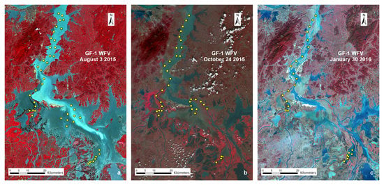
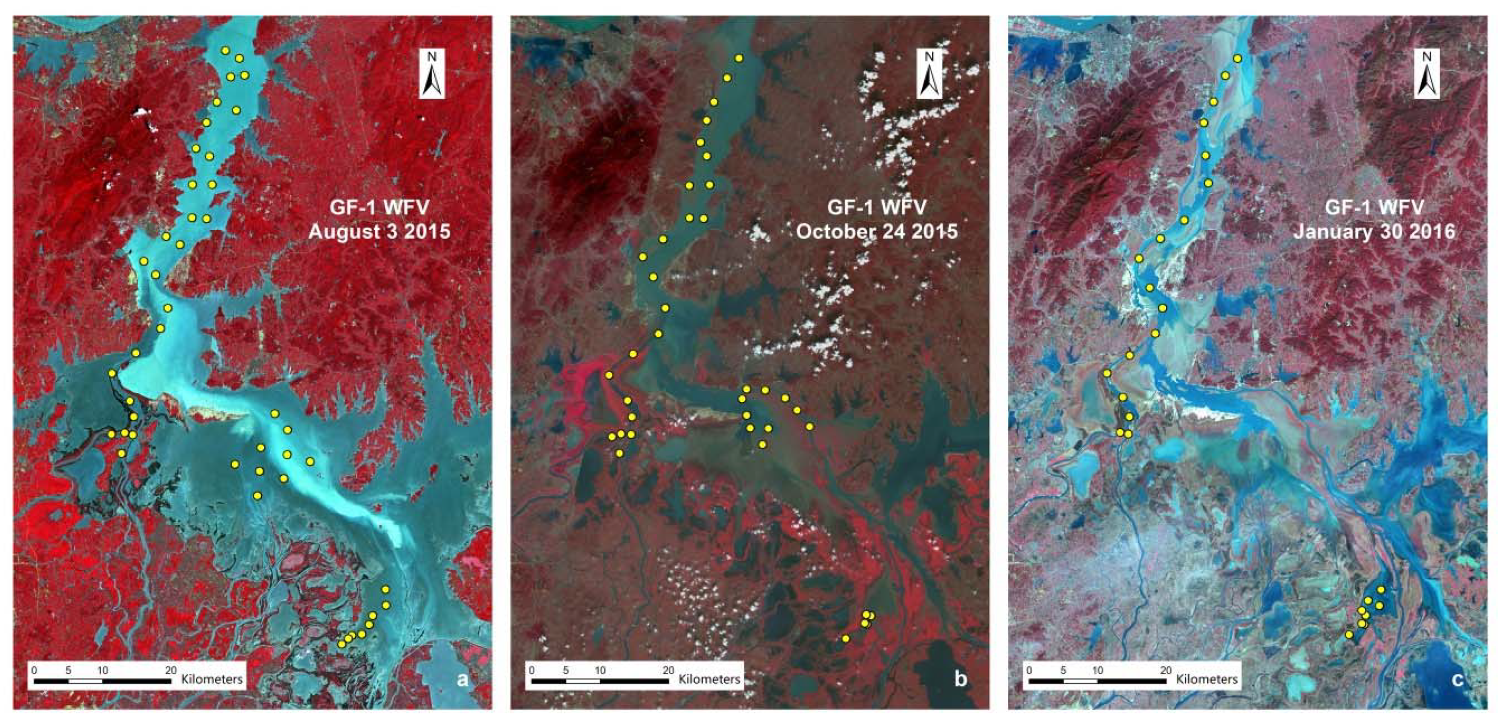
Field data were obtained from Poyang Lake in August 2015 (August 1, 3, and 5, 2015), October 2015 (October 23 and 24, 2015), and January 2016 (January 24 and 25, 2016), from 43, 33, and 26 sampling sites, respectively. Figure 2 shows the locations of the sampling sites. For each sampling exercise, water was collected from a water depth of between 0 and 50 cm. All of the samples were held on ice and stored for subsequent measurements of the concentrations of Chl-a and TSM in the laboratory. Two 500ml portions of each sample were used to filter for collecting Chl-a and TSM, respectively. Chl-a was collected while using Whatman GF/F filters (0.7 μm pore size) and extracted with hot ethanol [31]. The concentrations of Chl-a were determined by spectrophotometry using a UV-2600PC UV–vis spectrophotometer (Shimadzu, Inc., Koyto, Japan). Water samples for TSM measurement were filtered while using Whatman GF/C filters (1.2 μm pore size) under vacuum. Subsequently, the filters were weighed gravimetrically to determine the concentration of TSM. Water temperature and turbidity were measured at the sampling sites using a YSI6600 portable multi-parameter water meter (Yellow Springs Instruments, Inc., Yellow Springs, Ohio, USA).
Remote-sensing-reflectance spectra were measured above the water surface at wavelengths between 350 and 2500 nm (1 nm interval) while using a Fieldspec 4 spectroradiometer (Analytical Spectral Devices, Inc., Boulder, Colorado, USA), following standard protocols [32]. Measurements were performed between 10:00 and 14:00 on sunny windless days. A total of 66 sampling sites (35 for August 2015, 17 for October 2015, and 14 for January 2016) were measured for remote-sensing-reflectance spectra due to the limitation of measurement time. The radiances from water, sky, and a reference panel were measured at each water sampling site.
Remote sensing reflectance () was determined as the ratio of water-leaving radiance () to the total downwelling irradiance [].
where is the total upwelling radiance from water, is the skylight radiance, δ is a proportionality coefficient that relates to the reflected sky radiance determined when the detector viewed the water surface [33], is the radiance from the reference panel, and is the irradiance reflectance of the reference panel.
2.3. Model Development and Assessment
In this study, semi-analytical and empirical approaches were used for estimating the concentrations of Chl-a and TSM by sensitive indices. The retrieval algorithms were established through regression processes while using linear, quadratic polynomial, exponential, logarithmic, and power-law regression approaches. The goodness of fit was judged by the value of the coefficient of determination (R2). The water samples were measured for remote-sensing-reflectance spectra and concentrations of Chl-a and TSM and then numbered from 1 to n, with 1 representing the samples with the highest concentration of Chl-a/TSM and n representing the samples with the lowest concentration. Subsequently, one sample was selected every three sample numbers—i.e., samples 1, 4, 7, 10, …, were selected; the selected samples were then used for model validation, while the remaining samples were used for model calibration. The coefficient of determination (R2), root-mean-square error (RMSE), and mean relative percentage error (MRPE) between the measured and predicted values of Chl-a or TSM concentration were calculated to assess the fitting and validation accuracy. The RMSE and MRPE were determined while using equations (2) and (3), respectively:
where n is the number of samples.
2.4. Image Data and Preprocessing
The GF-1 satellite images were downloaded through the Remote Sensing Market Service Platform of the Chinese Academy of Sciences (http://www.rscloudmart.com). The GF-1 satellite was launched on 26 April 2013. The satellite has a sun-synchronous orbit with an altitude of 645 km, crossing the equator at 10:30 local time in a descending mode. The satellite carries panchromatic (2 m resolution) and multi-spectral (8 m resolution) sensor systems for high-resolution observation and four wide-field-of-view (WFV) sensors for large-scale observation. The four WFV sensors acquire multi-spectral data with a spatial resolution of 16 m, a revisit cycle of four days, and wide coverage (4 × 200 km). Table 1 shows the spectral bands of GF-1. The predicted service life of this satellite is five to eight years. The images that were employed in this study were acquired August 3 and October 24, 2015 and January 30, 2016, respectively. The images captured the lake wetland transition between the highest and lowest water levels in summer 2015 and the follow up winter. The water level change reflected the variation of aquatic environment, in particular for concentrations of Chl-a and TSM.
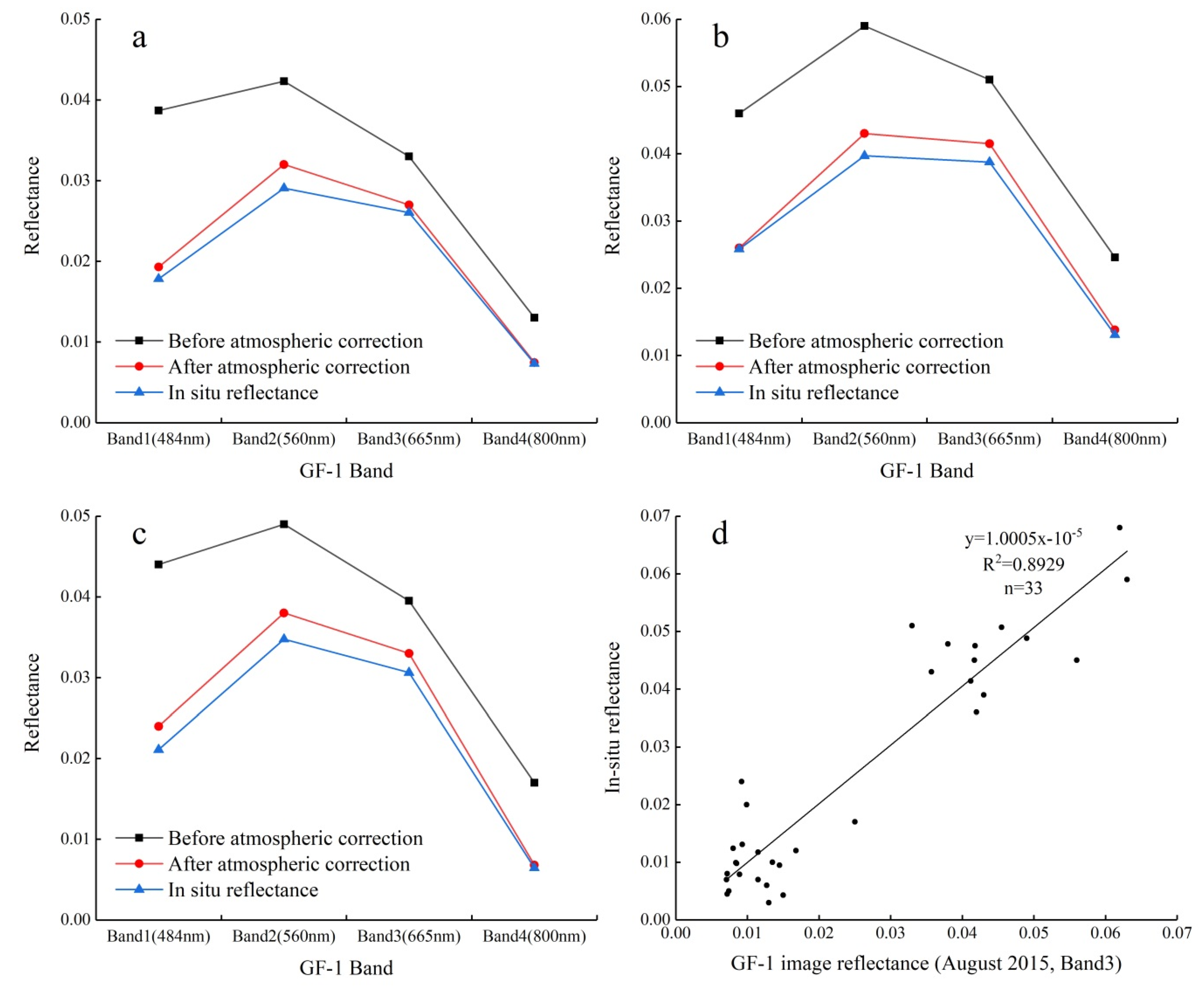
The preprocessing of GF-1 images includes geometric correction, radiometric calibration, atmospheric correction, and water body range extraction. In this paper, image data were processed while using the ENVI 5.3 software (Exelis Visual Information Solutions, Inc., Broomfield, Colorado, USA). Geometric correction was processed using the RPC (Rational Polynomial Coefficients) Orthorectification module in ENVI 5.3. The Landsat8 OLI panchromatic image covering the Poyang Lake area was used as a reference. The GF-1 images were then radiometrically calibrated to covert DN value to radiance. Atmospheric correction was performed while using the FLAASH (Fast Line-of-Sight Atmospheric Analysis of Spectral Hypercubes) module in ENVI 5.3. FLAASH integrates MODTRAN 5 radiative transfer model with all MODTRAN atmosphere and aerosol styles to provide a unique solution for each image [34]. In this study, the mid-latitude atmosphere and rural aerosol were selected in FLAASH to correct the GF-1 images. The results of atmospheric correction were the remote sensing reflectance above the water surface. Figure 3a–c show the comparison of GF-1 bands before and after atmospheric correction, along with in situ reflectance resampled according to GF-1 band configuration. Figure 3d presents the validation result between the Band-3 reflectance of GF-1 imagery and in situ measured reflectance from August 2015. The results showed that the atmospheric interference to sensor had been effectively removed through FLAASH implementation.
3. Results
3.1. In-Situ Data
Table 2 presents descriptive statistics for the measured concentrations of Chl-a and TSM in the water samples obtained from the three samplings on Poyang Lake.
The water reflectance spectra were obtained by calculating the radiance that was collected at the Poyang Lake sampling sites. After removing two abnormal spectral data (with extremely low reflectance) in August 2015 sampling, a total of 33 valid spectra were obtained for the August 2015 sampling, 17 valid spectra for the October 2015 sampling, and 14 valid spectra for the January 2016 sampling (Figure 4). The reflectance spectra show a reflectance peak between 550 and 600 nm, which is related to the weak absorption of chlorophyll and carotene. The absorption of cyanophycin leads to an absorption valley between 600 and 650 nm; however, this valley was not observed in the reflectance spectra in this study due to the low concentration of chlorophyll in Poyang Lake. However, we observed an obvious absorption between 660 and 680 nm, which is caused by chlorophyll in the red-light band. The absorption becomes more obvious as the concentration of chlorophyll increases. We also observed a reflection peak near 700 nm. This reflection peak is an important feature of algae-containing water, and its position and amplitude indicate the concentration of Chl-a, with the peak moving towards longer wavelengths as the concentration of Chl-a increases. The reflectance of the spectra is low after about 730 nm, which is due to the strong absorption of Chl-a in the near-infrared band. A small reflection peak appears near 820 nm, which may be due to the scattering of suspended matter. For some sampling sites, the peaks and valleys in the reflectance spectra are not strongly pronounced, which is mainly due to the low concentration of Chl-a and the high concentration of TSM. The measured reflectance spectra vary for different seasons due to the change in the lake’s water area throughout the year and the consequent change in the concentrations of Chl-a and TSM.
Of all the sampling sites that were used in this study, two sets of sampling sites were selected to determine the characteristic reflectance bands of Chl-a and TSM. Figure 5a shows reflectance spectra from three sampling sites with approximately the same Chl-a concentration (~4 mg/m3) and different TSM concentrations (18.6 mg/L, 55.8 mg/L, and 98.4 mg/L). Meanwhile, Figure 5b shows reflectance spectra from three sampling sites with similar TSM concentrations (~6 mg/L) and different Chl-a concentrations (3.91 mg/m3, 6.36 mg/m3, and 9.70 mg/m3).
From the spectra shown in Figure 5b, it can be concluded that the reflectance between 500 and 700 nm is inversely proportional to the concentration of Chl-a, and the reflectance beyond 700 nm is basically insensitive to the concentration of Chl-a. From the spectra that are shown in Figure 5a, it can be concluded that the reflectance is proportional to the TSM concentration. The wavelength positions of the absorption valley at the wavelength of 660 ~ 680nm and the reflection peak near 700nm are very stable, and they do not change with the change of TSM concentration. Therefore, the absorption valley at 660–680 nm and the reflection peak around 700 nm can be used as characteristic bands for the inversion of Chl-a concentration.
From the reflectance spectra that are shown in Figure 5a, it can be concluded that almost the whole reflectance of the spectra are significantly and positively correlated with TSM concentration between 350 and 900 nm. From the reflectance spectra that are shown in Figure 5b, it can be concluded that the reflectances below 700 nm are highly sensitive to Chl-a concentration. The reflectances beyond 700 nm are almost completely insensitive to Chl-a concentration, and the reflectance after 830 nm is weak and noisy. Therefore, it can be concluded that the reflectance between 700 and 830 nm can be used for the inversion of TSM concentration.
3.2. Inversion Model for Chlorophyll-a Concentration and Its Results
Figure 6 shows the Pearson correlation between normalized remote sensing reflectance and Chl-a concentration. The correlation varied significantly for different wavelengths.
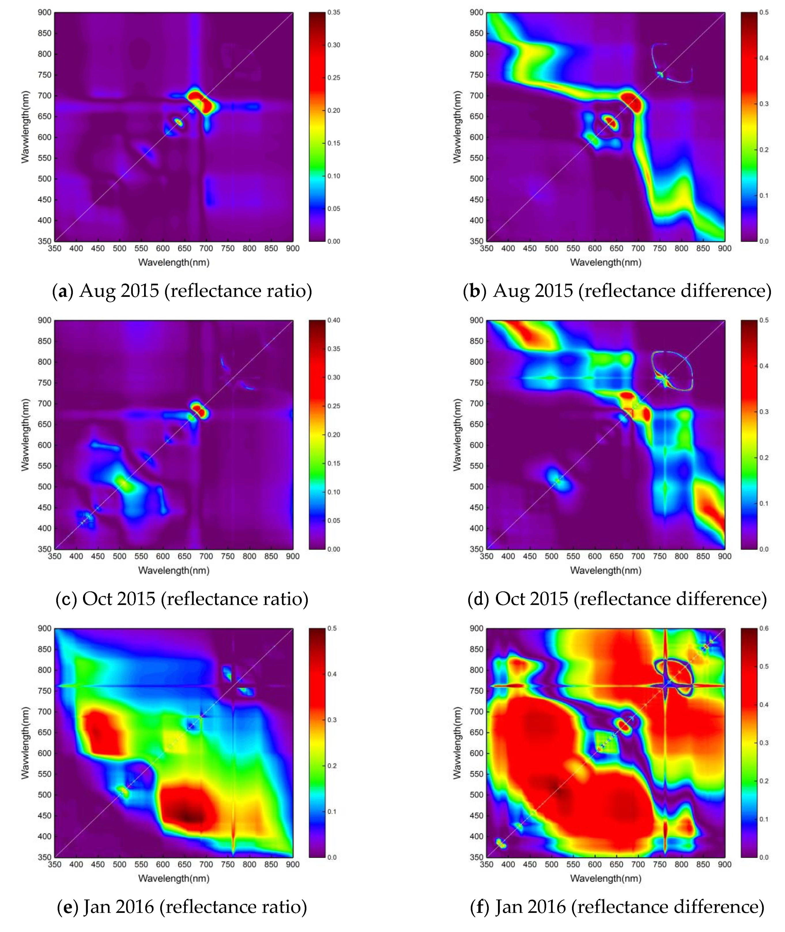
Subsequently, we constructed isopotential maps of the linear correlation coefficients of determination between the spectral indices and Chl-a concentration in the spectral interval 350–900 nm based on the original reflectance spectrum by establishing the spectral indices of reflectance difference and reflectance ratio and using the least squares method to iteratively regress the spectral indices and Chl-a concentrations of Poyang Lake.
3.2.1. Analytical Results for Spectral Data from August 2015
The coefficients of determination between the ratio index and Chl-a concentration in Poyang Lake are generally low, as shown in Figure 7a. The coefficients of determination for combination of wavelengths of 700–715 nm and 690–700 nm are relatively high, but they are still at a low level (highest R2=0.35). The coefficients of determination of the difference index for Chl-a concentration in Poyang Lake are higher than those of ratio index, as shown in Figure 7b. The combinations of spectral wavelengths that are sensitive to Chl-a concentration consist of the band near 650 nm and the band between 700 and 710 nm.
3.2.2. Analytical Results for Spectral Data from October 2015
As shown in the isopotential map that was based on the original spectral data from October 2015 shown in Figure 7c, the coefficients of determination between the Chl-a concentration and ratio index in Poyang Lake are low. High coefficients of determination are observed for spectral combination of wavelengths of 680–690 and 690–700 nm, however the maximum value (R2=0.4) is still at a low level. The coefficients of determination between difference index and Chl-a concentration in Poyang Lake are higher than those between ratio index and Chl-a concentration, as shown in Figure 7d. The combinations of spectral wavelengths those are sensitive to Chl-a are 660–680 vs 720–730nm and 390–420 vs 870–900 nm.
3.2.3. Analytical Results for Spectral Data from January 2016
The coefficients of determination for the original spectral data from January 2016, which reached a maximum value of 0.5, were higher than the coefficients of determination for the original spectral data from August and October 2015, as shown in Figure 7e. The spectral combinations with the highest coefficients of determination are 440–470 nm vs 630–700 nm. The coefficients of determination between difference index and Chl-a concentration in Poyang Lake are higher than those of the ratio index, as shown in Figure 7f. The combinations of spectral wavelengths that are sensitive to Chl-a concentration are (1) 450–500 vs 500–540 nm, (2) 450–500 vs 650–700 nm, and (3) 360–420 nm and 760 nm. Table 3 summarizes the combinations of spectral wavelengths with the highest spectral index fit in Figure 7.
Overall, the results of the analysis show that the coefficients of determination of the linear correlation between the ratio index and the Chl-a concentration were lower than the coefficient of determination of the linear correlation between the difference index and the Chl-a concentration. The difference index corresponds to a wider range of sensitive bands than the ratio index. The spectral wavelengths that were sensitive to Chl-a concentration mainly corresponded to bands 1, 3, and 4 of the GF-1 image, and the bands of the GF-1 images have good overlap with the MODIS image. El-Alem et al. [35] have found that an APPEL (APProach by ELimination) model while using the combination of MODIS bands 1, 2, and 3 can be used to determine the Chl-a concentration in water. The maximum reflectance of Chl-a is in the near-infrared region. Furthermore, colored dissolved organic matter (CDOM), TSM, and backscattering also affect reflectance in the near-infrared band. CDOM has the maximal reflection in the blue band, so the influence of CDOM can be eliminated in the blue band. TSM is highly sensitive in the red band. Therefore, the red band can eliminate the influence of TSM on the reflectance spectrum of Chl-a. Pure water has strong absorption characteristics in the red and near-infrared bands, so the influence of backscattering can be eliminated.
The APPEL model was established based on the spectral characteristics of Chl-a, pure water, TSM, and CDOM, as follows [35]:
The combination of GF-1 bands 1, 3, and 4 was used to establish the APPEL model. Table 4 shows the details of the models for the inversion of Chl-a concentration in different seasons.
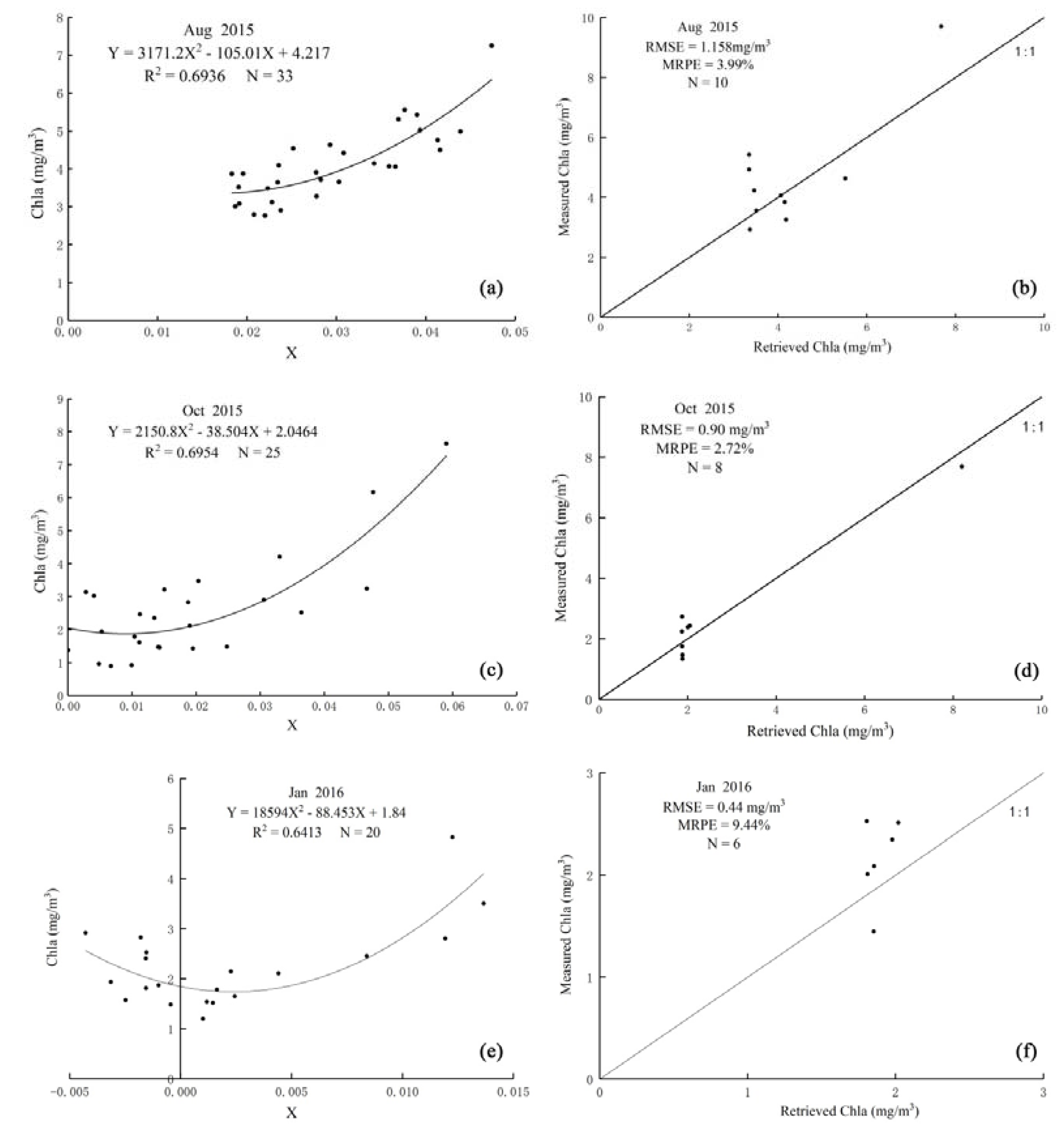
A summer inversion model for Chl-a concentration was established while using 33 sets of data that were measured in August 2015 (Figure 8a). Of the various models that were assessed, the inversion model that used quadratic polynomials had the highest fitting degree (R2=0.6936); this model was subsequently validated while using 10 sets of measured data (Figure 8b). The results showed that the RMSE of the model was 1.158 mg/m3 and the MRPE was 3.99%. Additionally, an autumn inversion model for Chl-a concentration (Figure 8c) was established based on 25 sets of data measured in October 2015. Again, the model that used quadratic polynomials had the highest fitting degree (R2=0.6954). This model was validated with eight sets of measured data (Figure 8d). The results showed that the RMSE of the model was 0.90 mg/m3 and the MRPE was 2.72%. Finally, a winter inversion model for Chl-a concentration was established while using 20 sets of data measured in January 2016 (Figure 8e). The model that used quadratic polynomials had the highest fitting degree (R2=0.6413). This model was validated using six sets of measured data (Figure 8f). The results showed that the RMSE was 0.44 mg/m3 and the MRPE was 9.44%.
The Chl-a concentration in the entire coverage of Poyang Lake was obtained while using the ENVI 5.3 software based on the results of the summer, autumn, and winter inversion models for Chl-a concentration (Table 3). Figure 9 shows the corresponding estimates of the spatial distribution of the Chl-a concentration in Poyang Lake for each of these three seasons.
Figure 9a shows the results of the Chl-a concentration inversion while using the GF-1 satellite image from August 2015. In the study area, August is a summer month and is also the flooding (wet) season with the highest water level. During this month, the water temperature of Poyang Lake rises, the water velocity is the slowest, and algal growth is rapid, which causes the Chl-a concentrations to be the highest of the year, i.e., 5–30 mg/m3. The highest concentrations of Chl-a are distributed in the waters near the shore of Poyang Lake and in the Nanji wetland national nature reserve in the south central of the lake.
Figure 9b shows the results of the Chl-a concentration inversion while using the GF-1 satellite image from October 2015. In October, which is an autumn month in the study area, the water level of Poyang Lake begins to decline and the water temperature to decrease. At this time, the estimated concentration of Chl-a in the lake decreased to between 2 and 15 mg/m3. The highest concentrations of Chl-a are distributed around the channel in the north of Poyang Lake mouth, which connects it to the Yangtze River, and in the main channel near the center of the lake.
Figure 9c shows the results of the Chl-a concentration inversion while using the GF-1 satellite image from January 2016. In the study area, January is a winter month and is also in dry season. During this month, algae grow slowly in Poyang Lake. The estimated concentration of Chl-a was generally low, ranging from 0–11 mg/m3, and the estimated distribution was more uniform than for August or October. The highest concentrations of Chl-a are distributed near the channel in the northern part of Poyang Lake, which connects it to the Yangtze River, and in the places where the Ganjiang, Fuhe, Xinjiang, Raohe, and Xiushui rivers flow into the lake.
3.3. Retrieval Models and Results for Total Suspended Matter Concentration
Figure 10 illustrates the Pearson correlations between normalized remote sensing reflectance and TSM concentration. The correlation coefficient shows obvious variation for different wavelengths.
Two peaks and valleys were observed in the correlation curve for August 2015 (summer), as shown in Figure 10. The two peaks are located at wavelengths of 660~730 nm and 760~820 nm, respectively, and the maximum values of the correlation coefficients for the peaks are 0.85 and 0.75, respectively. The two valleys are located at wavelengths of 350~400 nm and 500~550 nm, respectively, and the maximum values of the correlation coefficients for the valleys are –0.76 and –0.72, respectively. For the August 2015 correlation curve, the maximum correlation coefficient (0.85) appears at a wavelength of 710 nm, and the minimum correlation coefficient (–0.76) appears at a wavelength of 371 nm. The correlation curve for October 2015 (autumn) shows different trends at wavelengths below and above 650 nm, respectively. Below 650 nm, the correlation coefficient is negative, reaching its minimum value of –0.96 at a wavelength of 590 nm; above 650 nm, the correlation coefficient is positive, reaching a maximum value of 0.98 at a wavelength of 756 nm. In January 2016, the water reflectance spectra that was most sensitive to TSM concentration, was observed at a wavelength of 723 nm, with the maximum correlation coefficient of 0.95. These sensitive wavelengths most corresponded to band 3 of the GF-1 image. Therefore, band 3 of the GF-1 image was used in the model for the retrieval of TSM concentration. We assessed the performance of five mathematical models for retrieval, which used linear, quadratic polynomial, exponential, logarithmic, and power-law equations, respectively, and selected the best-fitting model (i.e., the one with the highest coefficient of determination, R2) as the retrieval model. Table 5 describes the selected models for different seasons.
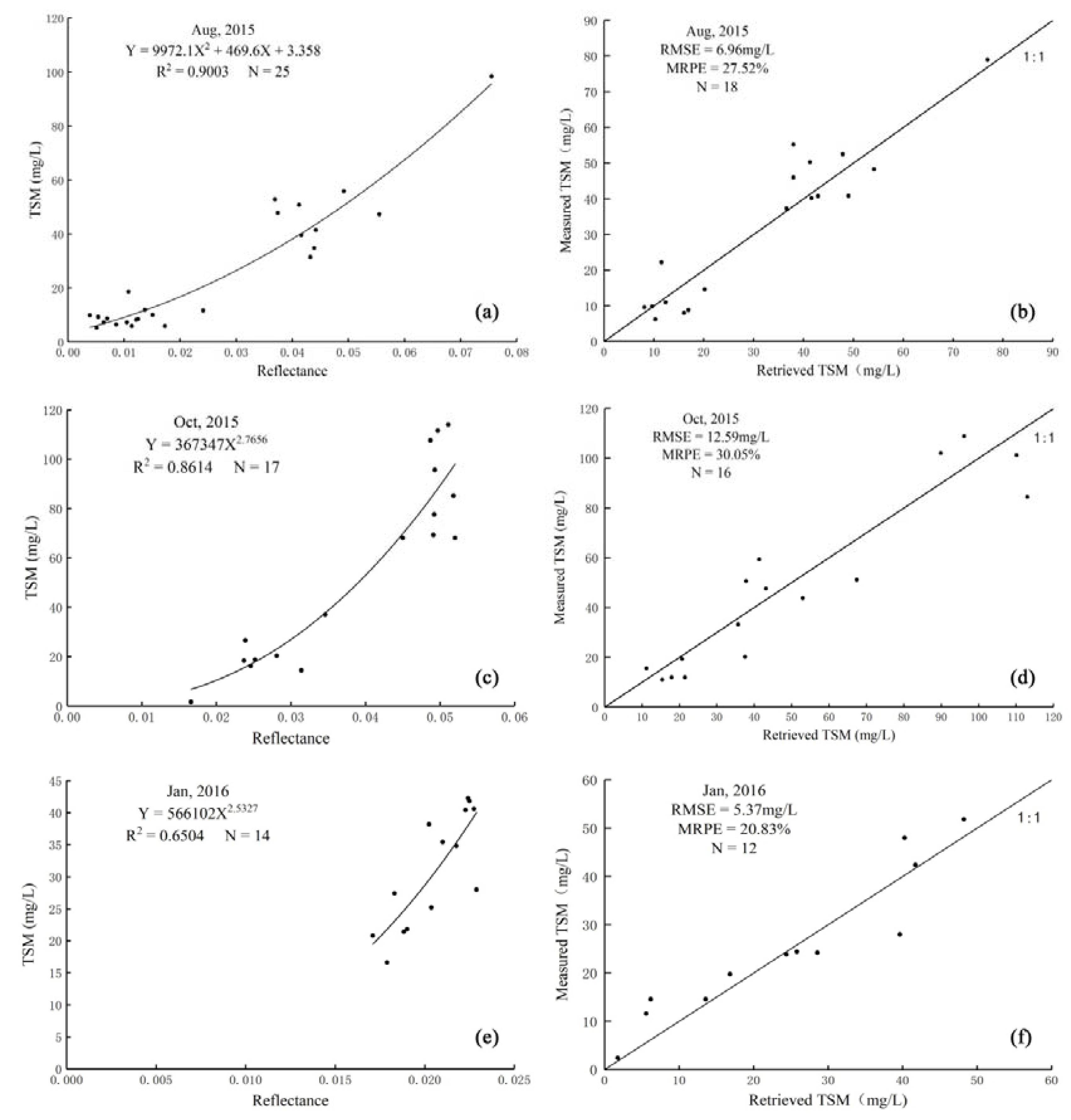
The field data that were measured in August 2015 were used to establish the summer retrieval model (Figure 11a). The retrieval model using a quadratic polynomial was found to have the best fit (R2=0.9003). This model was subsequently validated on 18 sets of measured data (Figure 11b). The results showed that the RMSE of the model was 6.96 mg/L and the MRPE was 27.52%. From the test results, it can be seen that the quadratic model in the single-band model predicted the summer TSM concentration of Poyang Lake well and the model had good stability.
The 17 sets of data that were measured in October 2015 were used to establish the autumn retrieval model (Figure 11c). The retrieval model using a power-law equation was found to have the best fit (R2=0.8614). The retrieval model was validated while using 16 sets of measured data (Figure 11d). The results showed that the RMSE of the model was 12.59 mg/L and the MRPE was 30.05%. It can be seen from the test results that the power-law model in the single-band model predicted the autumn TSM concentration of Poyang Lake well and the model had good stability.
The 14 sets of data that were measured in January 2016 were used to establish the winter retrieval model (Figure 11e). The retrieval model using the power-law equation was found to have the best fit (R2=0.6504). This retrieval model was validated while using 12 sets of measured data (Figure 11f). The results showed that the RMSE of the model was 5.37 mg/L and the MRPE was 20.83%. It can be seen from the test results that the power-law model in the single-band model predicted the winter TSM concentration of Poyang Lake well and the model had good stability.
The TSM concentrations for the whole of the Poyang Lake area were calculated while using the ENVI 5.3 software based on the results of the retrieval models for TSM concentration in summer (August 2015), autumn (October 2015), and winter (January 2016) (Table 4). Figure 12 shows a map showing the spatial distribution of TSM concentration in Poyang Lake.
Figure 12a shows the result of the retrieval of TSM concentration that is based on GF-1 image from August 2015. The overall level of TSM concentration in Poyang Lake was relatively low in August 2015, and the lowest TSM concentrations occurred in the eastern, western, and southern parts of Poyang Lake. The concentration of TSM in the eastern part of the lake was generally below 100 mg/L, the concentration at the junction of the Xiu River and the Ganjiang River ranged from 0~68 mg/L, and the concentration in Junshan Lake (which lies to the south of Poyang Lake) ranged from 0~46 mg/L. The concentration of TSM was relatively high in the channel, which connects the north of the lake to the Yangtze River, and in the main channel in the center of the lake, due to the influence of sand mining in Poyang Lake [36]. In the northern part of the lake, the TSM concentration ranged from about 59–80 mg/L. The highest TSM concentration that was observed in the central channel was 103 mg/L.
Figure 12b illustrated that the overall TSM concentration in Poyang Lake in October was significantly higher than that in August. The highest concentration of TSM (254.43 mg/L) was observed in the channel connecting the northern part of the lake to the Yangtze River. This can be attributed to the fact that, in August and September, increased rainfall in the Yangtze River causes the water level of the Yangtze River near Poyang Lake to increase, which suppresses water outflow from Poyang Lake and causes the water from the Yangtze River to flow back into the lake. This flow causes the TSM concentration of Poyang Lake to reach its highest levels in the channel connecting it with the Yangtze River due to the high concentration of TSM in the Yangtze River. The increases in TSM concentration that were observed in other parts of Poyang Lake can be attributed to the continuous sand mining activity in the lake area.
Figure 12c illustrated that the TSM concentration of Poyang Lake varied between 0 and 201 mg/L in January, i.e., the maximum TSM concentration higher than that in August 2015. The highest TSM concentrations were observed in the channel that connects the north of the lake with the Yangtze River, and in the main channel in the center of the lake.
4. Discussion
4.1. Spatial and Seasonal Variation of Chl-a
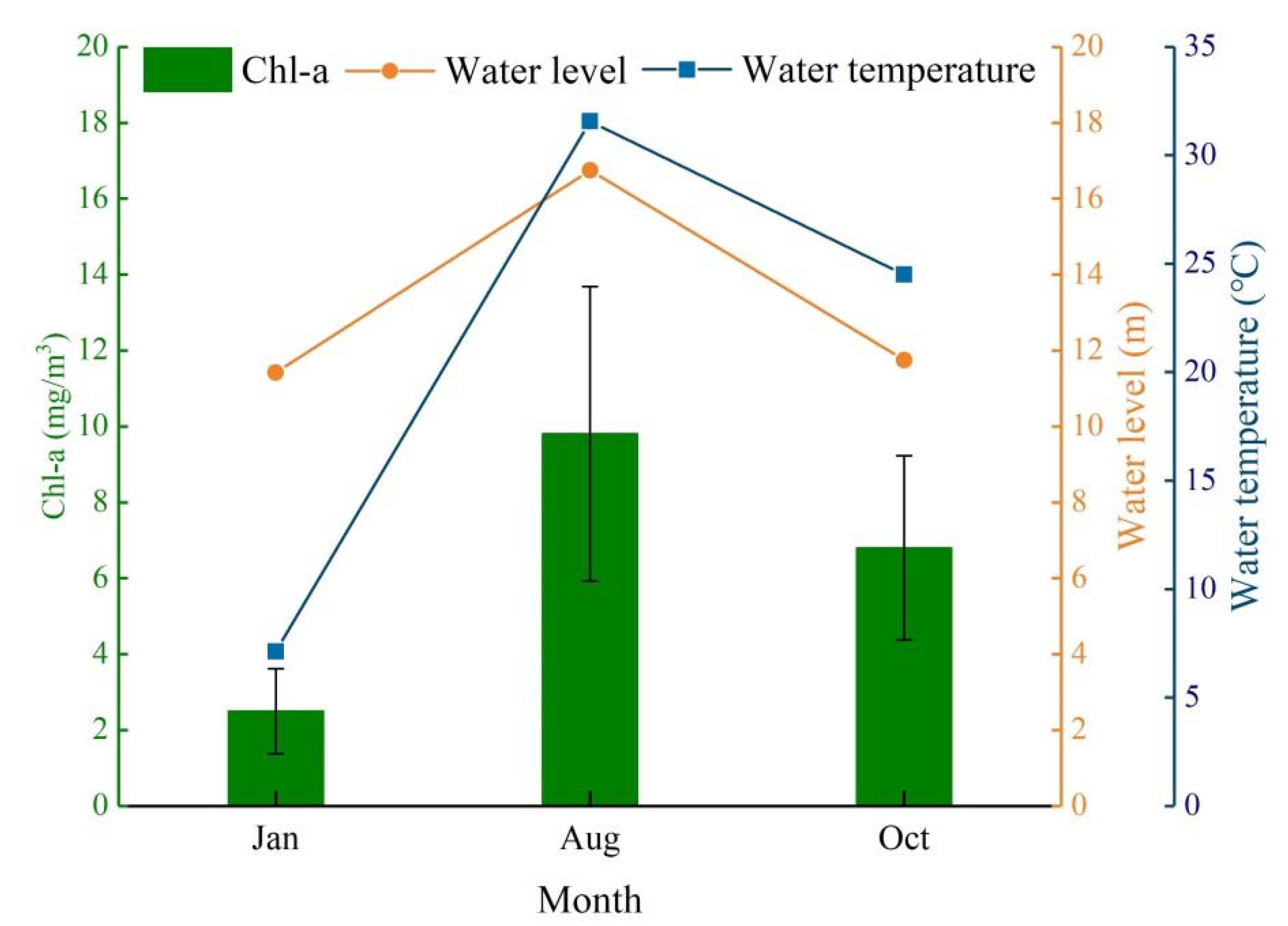
Figure 13 illustrates the water temperature data from the sampling sites in order to investigate the seasonal variation of the concentration of Chl-a in detail; the results of the inversion of the concentration of Chl-a; and the water level measured at the Xingzi hydrological station.
The comparison in Figure 13 suggested that, regarding the spatial distribution of Chl-a, the highest concentrations of Chl-a in Poyang Lake are mainly distributed near the channel in the north of the lake, which connects it to the Yangtze River, in the places where the Ganjiang, Fuhe, Xinjiang, Raohe, and Xiushui rivers flow into the lake, and in the waters near to the shore of the lake. These observations can be attributed to the transport of various pollutants into the lake by the Ganjiang, Fuhe, Xinjiang, Raohe, and Xiushui rivers, and to human activities in waters near to the lake shore [37]. Sand mining occurs during the whole year in the northern channel that connects the lake with the Yangtze River [16]. Consequently, a large amount of sewage is discharged from sand dredgers, and sand mining activities disturb the lake bottom, releasing large amounts of nutrients; both of these result in a high level of nutrients in the lake water, which in turn leads to an increase in the concentration of Chl-a [38]. The relatively high Chl-a concentration observed in the waters near the inlets of the five aforementioned rivers is mainly due to the large amount of pollutants carried by these rivers [39]. Large amounts of domestic and industrial wastewater are discharged into the lake due to the large numbers of people who live near the shores of Poyang Lake and the acceleration of industrialization and urbanization that has taken place in recent years; this discharge is also an important factor behind the increase of Chl-a concentration in the lake.
The temporal variation of Chl-a concentration in Poyang Lake is related to the lake’s unique hydrological characteristics. From Figure 13, the Chl-a concentration of Poyang Lake is positively correlated with water temperature and water level. This finding is similar to the analysis of Zheng et al [37]. In the study area, summer is part of the wet season and, accordingly, the water level reached its yearly maximum in August 2015. In the wet season, the increase in water level causes Poyang Lake to enter a relatively stable state, with the water flow speed reducing and the water temperature increasing. These two factors are highly conducive to the growth of algae in the water body, which causes the concentration of Chl-a in the lake to increase. This can explain our observation that summer is the season with the highest concentration of Chl-a. On the other hand, the water level of Poyang Lake begins to decline in autumn, the water flow speed increases, and the Yangtze River begins to flow into the lake, due to the fact that the level of the river is higher than that of Poyang Lake [40]; consequently, the water temperature begins to decline in autumn, which, in turn, causes the Chl-a concentration to reduce to levels that are significantly lower than those in summer. Winter is the season with the lowest water level and the lowest water temperature in Poyang Lake. The combination of these two factors inhibits the growth of algae in the lake, which in turn causes the concentration of Chl-a to reach its lowest yearly value during this season.
4.2. Spatial and Seasonal Variation of TSM
We compared the concentration of TSM calculated while using the retrieval model, the water temperature measured at the sampling sites, and the water level measured at the Xingzi hydrological station in order to investigate the seasonal variation of the TSM concentration in Poyang Lake (Figure 14).
Figure 12 concluded that the concentration of TSM was high in the channel that connects the north of Poyang Lake to the Yangtze River, and in the main central channel of the lake. This can be attributed to human activities, such as shipping and sand mining [16]. The TSM concentration in the Junshan Lake area (the south part of Poyang Lake) was at a low level throughout the year and changed little throughout the year. The concentration of TSM near the inlets of the Ganjiang, Fuhe, Xinjiang, Raohe, and Xiushui rivers changed greatly throughout the year. This can be attributed to the difference in the flow speed of these five rivers throughout the year [41].
Regarding the temporal variation of the concentration of TSM, the mean concentration was the lowest in summer (August 2015) [42]. At that time, water temperature and water level of Poyang Lake both reached their highest yearly levels. At this time, the flow speed of the lake was relatively low [41]. Although the concentration of TSM was high in the lake’s main central channel, which can be attributed to the impact of sand mining activities, the TSM concentration in most of the other areas of the lake was low and relatively homogenous. The highest TSM concentration that was observed in Poyang Lake in this study was 254.43 mg/L, and it was observed in autumn (October 2015). At this time, the water level of Poyang Lake began to retreat, and the water level of the Yangtze River was higher than that of Poyang Lake. The backflow of water from the Yangtze River into Poyang Lake and the influence of sand mining activities increased the concentration of TSM in Poyang Lake [27]. The highest TSM concentrations were mainly observed in the channel that connects the north of the lake to the Yangtze River, and in the central part of the lake. In winter month (January 2016), the water temperature and the water level reached their lowest yearly levels. At this time, the TSM concentration ranged from 0 to 201 mg/L. This can be attributed to human activities, such as shipping and sand mining, which disturb the sediment at the lake bottom and thereby lead to an increase in TSM concentration [27]. In January 2016, the highest concentrations of TSM were observed in the lake’s main central channel and in the channel that connects the north of the lake to the Yangtze River.
5. Conclusions
Images from the GF-1 satellite helped to establish retrieval models for concentrations of Chl-a and TSM in Poyang Lake in different seasons. The retrieval model that obtained the best fit for each season, respectively, was used to analyze the spatial and temporal variations of the concentrations of Chl-a and TSM for that season.
For Chl-a, the results showed that the wavelengths corresponding to bands 1, 3, and 4 of the GF-1 images were the most sensitive to changes in the concentration of Chl-a. Moreover, the APPEL model was used to establish the band combination, thus obtaining the retrieval models of Chl-a concentration for different seasons. The highest concentrations of Chl-a in Poyang Lake were mainly observed near the channel that connects the north of the lake to the Yangtze River, the places where the Ganjiang, Fuhe, Xinjiang, Raohe, and Xiushui rivers enter the lake, and near to the lake shore. In the central area of the lake, the concentration of Chl-a was relatively low and uniform. Regarding the temporal variation of Chl-a in Poyang Lake, the concentration was the highest in summer (August 2015), second-highest in autumn (October 2015), and lowest in winter (January 2016).
For TSM, the results showed that the correlation between the reflectance and TSM concentration was the highest for wavelengths corresponding to band 3 of the GF-1 satellite images. The highest TSM concentrations in Poyang Lake were mainly observed in the channel that connects the north of the lake to the Yangtze River, and in the lake’s main central channel. The TSM concentration in Junshan Lake was relatively low and it changed little between seasons. The TSM concentrations near the inlets of the Ganjiang, Fuhe, Xinjiang, Raohe, and Xiushui rivers to Poyang Lake were lower than that in the channel that connects the north of the lake to the Yangtze River. Regarding the temporal variation of TSM concentration in Poyang Lake, the concentration was highest in autumn (October 2015), second highest in winter (January 2016), and lowest in summer (August 2015).
Author Contributions
Conceptualization, J.X. and Y.W.; Methodology, J.X.; Software, C.G.; Investigation, J.X. and C.G.; Data curation, J.X. and C.G.; Writing—original draft preparation, J.X. and C.G.; Writing—review and editing, J.X. and Y.W.; Supervision, Y.W.; Funding acquisition, J.X. All authors have read and agreed to the published version of the manuscript.
Funding
This study was funded by the National Natural Science Foundation of China (grant no. 41471298), the Key Research and Development Project of Jiangxi Province (grant no. 20192ACB70014), the Opening Fund of Key Laboratory of Poyang Lake Wetland and Watershed Research (Jiangxi Normal University), Ministry of Education (grant no. PK2018002), the Science and Technology Project of Education Department of Jiangxi Province, and the Young Talents Project of Jiangxi Normal University.
Acknowledgments
We appreciate the insightful and constructive comments and suggestions from the anonymous reviewers and the Editor that helped improve the quality of the manuscript.
Conflicts of Interest
The authors declare no conflict of interest. The funders had no role in the design of the study; in the collection, analyses, or interpretation of data; in the writing of the manuscript, or in the decision to publish the results.
References
- Giardino, C.; Pepe, M.; Brivio, P.A.; Ghezzi, P.; Zilioli, E. Detecting chlorophyll, Secchi disk depth and surface temperature in a sub-alpine lake using Landsat imagery. Sci. Total Environ. 2001, 268, 19–29. [Google Scholar] [CrossRef]
- Ayenew, T. Environmental implications of changes in the levels of lakes in the Ethiopian Rift since 1970. Reg. Environ. Chang. 2004, 4, 192–204. [Google Scholar] [CrossRef]
- Wang, Y.; Qi, S.; Xu, J. Multitemporal remote sensing for inland water bodies and wetland monitoring. In Multitemporal Remote Sensing; Yifang Ban, Ed.; Springer: Cham, Switzerland, 2016; pp. 357–371. [Google Scholar]
- Liu, Y.; Islam, M.A.; Gao, J. Quantification of shallow water quality parameters by means of remote sensing. Prog. Phys. Geogr. 2003, 27, 24–43. [Google Scholar] [CrossRef]
- Wang, Y.; Yésou, H. Remote sensing of floodpath lakes and wetlands: A challenging frontier in the monitoring of changing environments. Remote Sens. 2018, 10, 1955. [Google Scholar] [CrossRef] [Green Version]
- Duan, H.; Zhang, Y.; Zhang, B.; Song, K.; Wang, Z. Assessment of chlorophyll-a concentration and trophic state for Lake Chagan using Landsat TM and field spectral data. Environ. Monit. Assess. 2007, 129, 295–308. [Google Scholar] [CrossRef] [PubMed]
- Miller, R.L.; Liu, C.-C.; Buonassissi, C.J.; Wu, A.-M. A multi-sensor approach to examining the distribution of total suspended matter (TSM) in the Albemarle-Pamlico estuarine system, NC, USA. Remote Sens. 2011, 3, 962–974. [Google Scholar] [CrossRef] [Green Version]
- Torbick, N.; Hu, F.; Zhang, J.; Qi, J.; Zhang, H.; Becker, B. Mapping chlorophyll-a concentrations in west lake, China using Landsat 7 ETM. J. Great Lakes Res. 2008, 34, 559–565. [Google Scholar] [CrossRef]
- Mishra, D.R.; Ogashawara, I.; Gitelson, A.A. Bio-Optical Modeling and Remote Sensing of Inland Waters; Elsevier: Amsterdam, The Netherlands, 2017. [Google Scholar]
- Zheng, Z.; Li, Y.; Guo, Y.; Xu, Y.; Liu, G.; Du, C. Landsat-based long-term monitoring of total suspended matter concentration pattern change in the wet season for Dongting Lake, China. Remote Sens. 2015, 7, 13975–13999. [Google Scholar] [CrossRef] [Green Version]
- Molkov, A.A.; Fedorov, S.V.; Pelevin, V.V.; Korchemkina, E.N. Regional models for high-resolution retrieval of chlorophyll a and TSM concentrations in the Gorky Reservoir by Sentinel-2 imagery. Remote Sens. 2019, 11, 1215. [Google Scholar] [CrossRef] [Green Version]
- Wang, M.; Shi, W. Satellite-observed algae blooms in China’s Lake Taihu. EosTransactions Am. Geophys. Union 2008, 89, 201–202. [Google Scholar] [CrossRef]
- Wang, M.; Shi, W.; Tang, J. Water property monitoring and assessment for China’s inland Lake Taihu from MODIS-Aqua measurements. Remote Sens. Environ. 2011, 115, 841–854. [Google Scholar] [CrossRef]
- Matthews, M.W. Eutrophication and cyanobacterial blooms in South African inland waters: 10years of MERIS observations. Remote Sens. Environ. 2014, 155, 161–177. [Google Scholar] [CrossRef]
- Feng, L.; Hu, C.; Han, X.; Chen, X.; Qi, L. Long-term distribution patterns of chlorophyll-a concentration in China’s largest freshwater lake: MERIS full-resolution observations with a practical approach. Remote Sens. 2014, 7, 275–299. [Google Scholar] [CrossRef] [Green Version]
- Feng, L.; Hu, C.; Chen, X.; Tian, L.; Chen, L. Human induced turbidity changes in Poyang Lake between 2000 and 2010: Observations from MODIS. J. Geophys. Res. Ocean. 2012, 117. [Google Scholar] [CrossRef]
- Shi, K.; Zhang, Y.; Zhu, G.; Liu, X.; Zhou, Y.; Xu, H.; Qin, B.; Liu, G.; Li, Y. Long-term remote monitoring of total suspended matter concentration in Lake Taihu using 250m MODIS-Aqua data. Remote Sens. Environ. 2015, 164, 43–56. [Google Scholar] [CrossRef]
- Salem, S.I.; Higa, H.; Kim, H.; Kazuhiro, K.; Kobayashi, H.; Oki, K.; Oki, T. Multi-algorithm indices and look-up table for chlorophyll-a retrieval in highly turbid water bodies using multispectral data. Remote Sens. 2017, 9, 556. [Google Scholar] [CrossRef] [Green Version]
- Van Nguyen, M.; Lin, C.-H.; Chu, H.-J.; Muhamad Jaelani, L.; Aldila Syariz, M. Spectral feature selection optimization for water quality estimation. Int. J. Environ. Res. Public Health 2020, 17, 272. [Google Scholar] [CrossRef] [PubMed] [Green Version]
- Zhou, L.; Roberts, D.A.; Ma, W.; Zhang, H.; Tang, L. Estimation of higher chlorophylla concentrations using field spectral measurement and HJ-1A hyperspectral satellite data in Dianshan Lake, China. ISPRS J. Photogramm. Remote Sens. 2014, 88, 41–47. [Google Scholar] [CrossRef]
- Matthews, M.W.; Bernard, S.; Robertson, L. An algorithm for detecting trophic status (chlorophyll-a), cyanobacterial-dominance, surface scums and floating vegetation in inland and coastal waters. Remote Sens. Environ. 2012, 124, 637–652. [Google Scholar] [CrossRef]
- Shen, F.; Zhou, Y.-X.; Li, D.-J.; Zhu, W.-J.; Suhyb Salama, M. Medium resolution imaging spectrometer (MERIS) estimation of chlorophyll-a concentration in the turbid sediment-laden waters of the Changjiang (Yangtze) Estuary. Int. J. Remote Sens. 2010, 31, 4635–4650. [Google Scholar] [CrossRef]
- Liu, H.; Li, Q.; Shi, T.; Hu, S.; Wu, G.; Zhou, Q. Application of Sentinel 2 MSI images to retrieve suspended particulate matter concentrations in Poyang Lake. Remote Sens. 2017, 9, 761. [Google Scholar] [CrossRef] [Green Version]
- Bresciani, M.; Cazzaniga, I.; Austoni, M.; Sforzi, T.; Buzzi, F.; Morabito, G.; Giardino, C. Mapping phytoplankton blooms in deep subalpine lakes from Sentinel-2A and Landsat-8. Hydrobiologia 2018, 824, 197–214. [Google Scholar] [CrossRef] [Green Version]
- Xu, J.; Fang, C.; Gao, D.; Zhang, H.; Gao, C.; Xu, Z.; Wang, Y. Optical models for remote sensing of chromophoric dissolved organic matter (CDOM) absorption in Poyang Lake. ISPRS J. Photogramm. Remote Sens. 2018, 142, 124–136. [Google Scholar] [CrossRef]
- de Leeuw, J.; Shankman, D.; Wu, G.; De Boer, W.F.; Burnham, J.; He, Q.; Yesou, H.; Xiao, J. Strategic assessment of the magnitude and impacts of sand mining in Poyang Lake, China. Reg. Environ. Chang. 2010, 10, 95–102. [Google Scholar] [CrossRef]
- Gao, J.H.; Jia, J.; Kettner, A.J.; Xing, F.; Wang, Y.P.; Xu, X.N.; Yang, Y.; Zou, X.Q.; Gao, S.; Qi, S. Changes in water and sediment exchange between the Changjiang River and Poyang Lake under natural and anthropogenic conditions, China. Sci. Total Environ. 2014, 481, 542–553. [Google Scholar] [CrossRef] [PubMed]
- Deng, X.; Zhao, Y.; Wu, F.; Lin, Y.; Lu, Q.; Dai, J. Analysis of the trade-off between economic growth and the reduction of nitrogen and phosphorus emissions in the Poyang Lake watershed, China. Ecol. Model. 2011, 222, 330–336. [Google Scholar] [CrossRef]
- Li, B.; Yang, G.; Wan, R.; Hörmann, G.; Huang, J.; Fohrer, N.; Zhang, L. Combining multivariate statistical techniques and random forests model to assess and diagnose the trophic status of Poyang Lake in China. Ecol. Indic. 2017, 83, 74–83. [Google Scholar] [CrossRef]
- Xu, J.; Wang, Y.; Gao, D.; Yan, Z.; Gao, C.; Wang, L. Optical properties and spatial distribution of chromophoric dissolved organic matter (CDOM) in Poyang Lake, China. J. Great Lakes Res. 2017, 43, 700–709. [Google Scholar] [CrossRef]
- Lorenzen, C.J. Determination of chlorophyll and pheo-pigments: Spectrophotometric equations. Limnol. Oceanogr. 1967, 12, 343–346. [Google Scholar] [CrossRef]
- Mueller, J.; Fargion, G. Ocean Optics Protocols for Satellite Ocean Color Sensor Validation, Revision 3; Goddard Space Flight Center: Greenbelt, Maryland, 2002.
- Mobley, C.D. Estimation of the remote-sensing reflectance from above-surface measurements. Appl. Opt. 1999, 38, 7442–7455. [Google Scholar] [CrossRef]
- Song, K.; Li, L.; Wang, Z.; Liu, D.; Zhang, B.; Xu, J.; Du, J.; Li, L.; Li, S.; Wang, Y. Retrieval of total suspended matter (TSM) and chlorophyll-a (Chl-a) concentration from remote-sensing data for drinking water resources. Environ. Monit. Assess. 2012, 184, 1449–1470. [Google Scholar] [CrossRef] [PubMed]
- El-Alem, A.; Chokmani, K.; Laurion, I.; El-Adlouni, S.E. Comparative analysis of four models to estimate chlorophyll-a concentration in case-2 waters using moderate resolution imaging spectroradiometer (MODIS) imagery. Remote Sens. 2012, 4, 2373–2400. [Google Scholar] [CrossRef] [Green Version]
- Yao, J.; Zhang, D.; Li, Y.; Zhang, Q.; Gao, J. Quantifying the hydrodynamic impacts of cumulative sand mining on a large river-connected floodplain lake: Poyang Lake. J. Hydrol. 2019, 579, 124156. [Google Scholar] [CrossRef]
- Zheng, L.; Wang, H.; Huang, M.; Liu, Y. Relationships between temporal and spatial variations of water quality and water level changes in Poyang Lake based on 5 consecutive years’ monitoring. Appl. Ecol. Environ. Res. 2019, 17, 11687–11699. [Google Scholar] [CrossRef]
- Wu, Z.; He, H.; Cai, Y.; Zhang, L.; Chen, Y. Spatial distribution of chlorophyll a and its relationship with the environment during summer in Lake Poyang: A Yangtze-connected lake. Hydrobiologia 2014, 732, 61–70. [Google Scholar] [CrossRef]
- Wu, Z.; Cai, Y.; Liu, X.; Xu, C.P.; Chen, Y.; Zhang, L. Temporal and spatial variability of phytoplankton in Lake Poyang: The largest freshwater lake in China. J. Great Lakes Res. 2013, 39, 476–483. [Google Scholar] [CrossRef]
- Wu, Z.; Zhang, D.; Cai, Y.; Wang, X.; Zhang, L.; Chen, Y. Water quality assessment based on the water quality index method in Lake Poyang: The largest freshwater lake in China. Sci. Rep. 2017, 7, 1–10. [Google Scholar] [CrossRef]
- Gu, C.; Mu, X.; Gao, P.; Zhao, G.; Sun, W.; Li, P. Effects of climate change and human activities on runoff and sediment inputs of the largest freshwater lake in China, Poyang Lake. Hydrol. Sci. J. 2017, 62, 2313–2330. [Google Scholar] [CrossRef]
- Wang, J.; Chen, E.; Li, G.; Zhang, L.; Cao, X.; Zhang, Y.; Wang, Y. Spatial and temporal variations of suspended solid concentrations from 2000 to 2013 in Poyang Lake, China. Environ. Earth Sci. 2018, 77, 590. [Google Scholar] [CrossRef]
Figure 1.
Map of Poyang Lake, China.

Figure 2.
Pseudocolor renderings of images from the Gaofen-1 (GF-1) satellite (a: 770–890 nm, b: 630-690 nm, c: 520–590 nm) showing the landscape of the study area at approximately the time that the field samplings were performed.
Figure 2.
Pseudocolor renderings of images from the Gaofen-1 (GF-1) satellite (a: 770–890 nm, b: 630-690 nm, c: 520–590 nm) showing the landscape of the study area at approximately the time that the field samplings were performed.

Figure 3.
Comparison of GF-1 reflectance before and after atmospheric correction with in situ measured spectra, (a): mean value of data from August 2015; (b): mean value of data from October 2015; and, (c): mean value of data from January 2016. (d) Validation between the Band-3 reflectance of GF-1 imagery and in situ measured reflectance (August 2015).

Figure 4.
Measured water reflectance spectra for (a) August 2015, (b) October 2015, and (c) January 2016.
Figure 4.
Measured water reflectance spectra for (a) August 2015, (b) October 2015, and (c) January 2016.

Figure 5.
(a) The measured remote-sensing-reflectance spectra of the surface of Poyang Lake for sites with similar concentrations of Chl-a and different concentrations of TSM. (b) The measured remote-sensing-reflectance spectra of the surface of Poyang Lake for sites with similar concentrations of TSM and different concentrations of Chl-a.

Figure 6.
Pearson correlation coefficient (R) between normalized reflectance and Chl-a concentration.
Figure 6.
Pearson correlation coefficient (R) between normalized reflectance and Chl-a concentration.

Figure 7.
Linear correlation coefficients between the spectral index and Chl-a concentration. (a) August 2015 data (reflectance ratio). (b) August 2015 data (reflectance difference). (c) October 2015 data (reflectance ratio). (d) October 2015 data (reflectance difference). (e) January 2016 data (reflectance ratio). (f) January 2016 data (reflectance difference).

Figure 8.
Test results for inversion models for Chl-a concentration for different periods: (a,b) calibration and validation results for August 2015; (c,d) calibration and validation results for October 2015; (e,f) calibration and validation results for January 2016. RMSE: root-mean-square error. MRPE: mean relative percentage error. R2: coefficient of determination.

Figure 9.
The estimated Chl-a concentration in Poyang Lake during (a) August 2015, (b) October 2015, and (c) January 2016, obtained from GF-1 satellite images using polynomial inversion models.
Figure 9.
The estimated Chl-a concentration in Poyang Lake during (a) August 2015, (b) October 2015, and (c) January 2016, obtained from GF-1 satellite images using polynomial inversion models.

Figure 10.
The Pearson correlation (R) between normalized remote sensing reflectance and TSM concentration.
Figure 10.
The Pearson correlation (R) between normalized remote sensing reflectance and TSM concentration.

Figure 11.
Test results for the models for the retrieval of TSM concentration for three seasons: (a,b) calibration and validation results for August 2015; (c,d) calibration and validation results for October 2015; (e,f) calibration and validation results for January 2016.
Figure 11.
Test results for the models for the retrieval of TSM concentration for three seasons: (a,b) calibration and validation results for August 2015; (c,d) calibration and validation results for October 2015; (e,f) calibration and validation results for January 2016.

Figure 12.
The estimated spatial distribution of TSM concentration in Poyang Lake for three periods: (a) August 2015; (b) October 2015; and, (c) January 2016.
Figure 12.
The estimated spatial distribution of TSM concentration in Poyang Lake for three periods: (a) August 2015; (b) October 2015; and, (c) January 2016.

Figure 13.
Relationship between Chl-a concentration, water temperature, and water level in Poyang Lake.
Figure 13.
Relationship between Chl-a concentration, water temperature, and water level in Poyang Lake.

Figure 14.
Plot showing the TSM concentration, water temperature, and water level of Poyang Lake.


Table 1.
Spectral bands of GF-1.
| Tag | Band Order | Wavelength (nm) | Description |
|---|---|---|---|
| Panchromatic system | Pan | 450–900 | Panchromatic |
| Multi-spectral system | Band 1 | 450–520 | Blue |
| Multi-spectral system | Band 2 | 520–590 | Green |
| Multi-spectral system | Band 3 | 630–690 | Red |
| Multi-spectral system | Band 4 | 770–890 | Near infrared |
Table 2.
Descriptive statistics for the measured concentrations of chlorophyll-a (Chl-a) and total suspended matter (TSM) in Poyang Lake.
Table 2.
Descriptive statistics for the measured concentrations of chlorophyll-a (Chl-a) and total suspended matter (TSM) in Poyang Lake.
| Sampling Date | Number of Samples | Statistics | Chl-a Concentration (mg/m3) | TSM Concentration (mg/L) |
|---|---|---|---|---|
| August 2015 (Summer) | 43 | Max | 20.54 | 98.40 |
| Min | 0.48 | 5.20 | ||
| Mean | 5.16 | 28.23 | ||
| SD | 3.88 | 22.49 | ||
| C.V. | 75.17% | 79.67% | ||
| October 2015 (Autumn) | 33 | Max | 11.43 | 114.00 |
| Min | 0.37 | 1.60 | ||
| Mean | 3.10 | 52.20 | ||
| SD | 2.43 | 35.79 | ||
| C.V. | 78.64% | 68.56% | ||
| January 2016 (Winter) | 26 | Max | 5.02 | 66.25 |
| Min | 0.80 | 2.40 | ||
| Mean | 2.32 | 29.94 | ||
| SD | 1.12 | 14.03 | ||
| C.V. | 48.33% | 46.86% |
Note: SD is the standard deviation; C.V. is the coefficient of variation.
Table 3.
Spectral response characteristics of Chl-a in Poyang Lake.
| Data Collection Date | Spectral Index | w1 (nm) | w2 (nm) | R2 |
| August 2015 | Reflectance Ratio (Rw1/Rw2) | 691 | 683 | 0.35 |
| Reflectance Difference (Rw1-Rw2) | 693 | 695 | 0.50 | |
| October 2015 | Reflectance Ratio (Rw1/Rw2) | 689 | 671 | 0.39 |
| Reflectance Difference (Rw1-Rw2) | 770 | 737 | 0.49 | |
| January 2016 | Reflectance Ratio (Rw1/Rw2) | 651 | 430 | 0.48 |
| Reflectance Difference (Rw1-Rw2) | 762 | 403 | 0.58 |
Note: R2 is coefficient of determination between spectral index and Chl-a concentration.
Table 4.
Details of the inversion models for the concentration of Chl-a.
| Date | Model Expression | Goodness of Fit (Coefficient of Determination, R2) |
| August 2015 (Summer) | Y = 3171.2X2 – 105.01X + 4.217 | 0.6936 |
| October 2015 (Autumn) | Y = 2150.8X2 – 38.504X + 2.0464 | 0.6954 |
| January 2016 (Winter) | Y = 18594X2 – 88.453X + 1.84 | 0.6413 |
Note: X is calculated by the APPEL (APProach by ELimination) model: X = R(B4) - [(R(B1) - R(B4)) * R(B4) + (R(B3) - R(B4))], R(Bn) represents the reflectance of band n of the GF-1 image.
Table 5.
Selected models for the retrieval of TSM concentration.
| Date | Model Expression | Goodness of Fit (Coefficient of Determination, R2) |
|---|---|---|
| August 2015 (summer) | Y = 9972.1X2 + 469.6X + 3.358 | 0.9003 |
| October 2015 (autumn) | Y = 367347X2.7656 | 0.8614 |
| January 2016 (winter) | Y = 566102X2.5327 | 0.6504 |
Note: Y represents the TSM concentration; X represents the reflectance of band 3 of the GF-1 image.
© 2020 by the authors. Licensee MDPI, Basel, Switzerland. This article is an open access article distributed under the terms and conditions of the Creative Commons Attribution (CC BY) license (http://creativecommons.org/licenses/by/4.0/).
Share and Cite
MDPI and ACS Style
Xu, J.; Gao, C.; Wang, Y. Extraction of Spatial and Temporal Patterns of Concentrations of Chlorophyll-a and Total Suspended Matter in Poyang Lake Using GF-1 Satellite Data. Remote Sens. 2020, 12, 622. https://doi.org/10.3390/rs12040622
AMA Style
Xu J, Gao C, Wang Y. Extraction of Spatial and Temporal Patterns of Concentrations of Chlorophyll-a and Total Suspended Matter in Poyang Lake Using GF-1 Satellite Data. Remote Sensing. 2020; 12(4):622. https://doi.org/10.3390/rs12040622
Chicago/Turabian StyleXu, Jian, Chen Gao, and Yeqiao Wang. 2020. "Extraction of Spatial and Temporal Patterns of Concentrations of Chlorophyll-a and Total Suspended Matter in Poyang Lake Using GF-1 Satellite Data" Remote Sensing 12, no. 4: 622. https://doi.org/10.3390/rs12040622
Note that from the first issue of 2016, this journal uses article numbers instead of page numbers. See further details here.