Characterizing the Spatial Variations of Forest Sunlit and Shaded Components Using Discrete Aerial Lidar
by
 and
and
Xiaofei Wang
1,2, 
Guang Zheng
1,*,
Zengxin Yun
1,3,
Zhaoshang Xu
1,3,
L. Monika Moskal
4 and
and
Qingjiu Tian
1 1
International Institute for Earth System Science, Nanjing University, Nanjing 210023, China
2
Collaborative Innovation Center of South China Sea Studies, Nanjing University, Nanjing 210023, China
3
Jiangsu Provincial Key Laboratory of Geographic Information Science and Technology, Nanjing 210023, China
4
Remote Sensing and Geospatial Analysis Laboratory, Precision Forestry Cooperative, School of Environment and Forest Science, University of Washington, Box 352100, Seattle, WA 98195, USA
*
Author to whom correspondence should be addressed.
Remote Sens. 2020, 12(7), 1071; https://doi.org/10.3390/rs12071071
Submission received: 27 February 2020
/
Revised: 21 March 2020
/
Accepted: 24 March 2020
/
Published: 26 March 2020
(This article belongs to the Section Forest Remote Sensing)
Abstract
:Forest three-dimensional (3-D) structure, in the vertical dimension, consists of at least two components, including overstory and a forest background matrix (i.e., shrubs, grass, and bare earth). Quantitatively characterizing the proportions of forest sunlit (i.e., sunlit overstory and forest background) and shaded (i.e., shaded overstory and forest background) components is a crucial step in simulating the spatial variations of bidirectional reflectance distribution function (BRDF) of a forest canopy. By developing a Voxel-based sorest sunlit and shaded (VFSS) approach driven by aerial laser scanning data (ALS), we investigated the spatial variations of the forest sunlit and shaded components in a heterogeneous urban forest park (Washington Park Arboretum) with abundant tree species and a homogeneous natural forest area (Panther Creek). Meanwhile, we validated the forest canopy directional reflectance at both solar principal and perpendicular planes at the plot level. Moreover, we explored the effects of ALS data characteristics and forest stand conditions on the estimation accuracy of forest sunlit and shaded components. Our results show that (1) ALS data effectively stratify overstory and forest background with the accuracy decreasing from 87% to 65% as forest densities increase; (2) the root mean square errors (RMSEs) between the modeled- and ALS-based proportions of forest sunlit and shaded components range from 5.8% to 11.1% affected by forest densities; and (3) the scan angles and flight directions have apparent effects on the estimation accuracy of forest sunlit and shaded components. This work provides a solid foundation to investigate the spatial variations of directional forest canopy reflectance with a high spatial resolution of 1 m.

1. Introduction
The anisotropic characteristics of forest canopy reflectance from multiple observation directions are greatly affected by the proportions of visible sunlit and shaded components in a forest stand [1,2,3]. The shaded/sunlit proportions also affect the estimation accuracy of gross primary production (GPP) using light use efficiency (LUE) models which are sensitive to the shaded/sunlit proportions [4,5]. A forest stand consists of overstory and forest background matrix, including shrubs, grass, and bare earth in a vertical way. It can be divided into four components as follows: Sunlit overstory, sunlit forest background, shaded overstory, and shaded forest background [6,7,8] under the specific observation geometry. The four component proportions directly determine the forest canopy spectral characteristics [9] and further affect the retrieval accuracy of forest leaf area index (LAI) [10,11] and chlorophyll content [12]. Then characterizing the sunlit and shaded components in a forest stand will be beneficial to the calculation of C assimilation and transpiration using advanced ecosystem models [13].
Most of the methods quantifying four forest components usually fall into three categories: (1) GO models: Various geometric optical (GO) models have been developed to compute the proportions of four forest components and bidirectional reflectance distribution function (BRDF) analytically or empirically [1,14,15,16,17]. However, there still exist some difficulties and challenges as follows: (i) The assumption that tree crowns have uniform shapes limits their applications in a heterogeneous forest stand with various tree species. Moreover, it is difficult to approximate the actual mutual shadowing effect between tree crowns using a statistical model and determining the unknown parameters of statistical models characterizing tree spatial distribution patterns.(ii) Most of the GO models are only used in relatively flat or slope areas, which prevent their applications in mountain areas [18,19]. However, the topographic variations affect proportions of the four forest components, further affecting the BRDF of a forest canopy [18,19,20]. (2) Ray-tracing algorithm: The ray-tracing based methods have been successfully developed during the past decades, such as deterministic ray-tracing [20], Monte Carlo ray-tracing model [21], and discrete anisotropic radiative transfer model (DART) [22]. Compared to the GO models, DART can simulate complex forest scenes through the importation of 3D trees generated in external modeling software or using turbid layers with defined crown structure parameters [23]. However, it is difficult to reconstruct the same virtual forest scene with the real forest plot used in DART software, which will introduce apparent errors to the estimation and simulation of the four forest components and BRDF [24,25]. (3) Spectral mixture analysis: The reflectance of a remotely sensed image pixel can be expressed as the weighted linear combinations of reflectance values of the sunlit forest canopy, sunlit forest background, and all shaded components based on the spectral mixture analysis [9,26,27,28]. However, similar spectral characteristics make it challenging to separate the shaded forest components and further obtain the proportions of four forest components in any observation direction using given optical imagery [28,29]. Thus, a more flexible and generic approach is needed to characterize the spatial variations of the four forest components based on the real forest three-dimensional (3D) scene.
The 3D structural information within the aerial laser scanning (ALS) data make it possible to characterize canopy structure [30,31] and separate overstory and forest background [32] quantitatively. Various structural parameters, such as crown size [33,34], tree height and location [35,36], canopy cover [37], and LAI [38], have been successfully obtained from ALS data. Latifi [39] found that ALS data outperformed other remotely sensed data in predicting forest structure parameters. Further, the detailed vertical structure [40] and shadowing effects among tree crowns implicitly contained within ALS data allow us to estimate the proportions of four forest components without using a statistical-based method. Meanwhile, the ALS-based digital elevation model with high spatial resolution [41,42,43] can be beneficial to accurately estimate the proportions of the four forest components. Hilker et al. [44] derived the shaded component proportion of forest canopy using a hillshade algorithm [45] from airborne Lidar data. However, few studies have paid attention to estimating the four forest component proportions of a forest stand with a real 3D forest scene using the ALS data. An ALS-based approach is needed to quantify the proportions of the four forest components. Additionally, the effects of ALS data characteristics and forest structure on the four forest component proportions estimation are still not clear. Therefore, our specific goals are:
(1) To develop an ALS-based method to estimate and validate the four forest component proportions of a forest scene and
(2) To investigate the spatial variations of the proportions of the four forest components, and further explore the factors affecting the estimation accuracy of the four forest components.
2. Materials and Methods
2.1. Study Sites
Two study sites were selected in this study. The first study site was the Washington Park Arboretum (WPA), which is located at the south of the University of Washington campus in Seattle, Washington, USA. It is an urban heterogeneous forest park. The dominant tree species include Douglas fir (Pseudotsuga menziesii), western hemlock (Tsuga heterophylla), western red cedar (Thuja plicata), bigleaf maple (Acer macrophyllum), monkey puzzle (Araucaria araucana), southern magnolia (Magnolia grandiflora), and New Mexican locust (Robinia Neomexicana). The terrain slope throughout the WPA site is less than 15%. The second study site was the Panther Creek (PC) watershed, which is a natural forest located at the southeast of the city of Portland, Oregon, U.S.A. It is a managed natural forested area. The Douglas fir (Pseudotsuga menziesii), western hemlock (Tsuga heterophylla), western red cedar (Thuja plicata), and bigleaf maple (Acer macrophyllum) are dominant tree species (Figure 1). The slope of the PC site was up to 51.3°.
We established four circular plots (i.e., WPA-P1, WPA-P2, WPA-P3, and WPA-P4) with a radius of 30 m in the WPA site, and three square plots (i.e., PC-P1, PC-P2, and PC-P3) with a side length of 40 m in the PC site based on the ground measurement data. According to forest densities’ variations, we selected four plots (i.e., WPA-P1, WPA-P2, WPA-P3, and PC-P1) to validate the ALS-based four forest component results. Meanwhile, three plots (i.e., WPA-P4, PC-P2, and PC-P3) were selected to explore the effects of ALS data characteristics on the estimation of the four forest component proportions resulting from a range of acquisitions of ALS data in these plots. Moreover, to investigate the effects of surrounding forest stands on the four forest component proportions estimation of a given forest stand, we constructed a plot (i.e., WPA-P2E) by extending the radius of plot WPA-P2 to 90 m. Based on the values of normalized difference vegetation index (NDVI) of pixels of the HyMap hyperspectral imagery, these forest plots were divided into three levels: Low density (i.e., 0.1 < NDVI < 0.3), medium density (i.e., 0.3 < NDVI < 0.5), and high density (i.e., NDVI > 0.5).More detailed characteristics of the plots can be found in Table 1.
2.2. Datasets
2.2.1. Field Data
We randomly selected 378 trees in the WPA site to measure the stem location and tree height using the Global Navigation Satellite System (GNSS), working with a differential mode and laser range finder in August 2009. We collected tree crown diameter measurements in two cross directions (North-South and West-East) for each tree crown. In the PC site, we measured tree height and stem location for each tree in the plots PC-P2 and PC-P3 in July 2009. There were 22 and 50 trees in the two plots, respectively.
2.2.2. Aerial Laser Scanning (ALS) Data
We acquired the ALS data for the WPA site in August 2008 using a Riegl LMS-Q560 (Riegal, Co. Ltd. Horn, Austria) laser scanner with a pulse frequency of 133,000 Hz. The flight height ranged from 145 m to 412 m, and the average elevation was about 310 m. The average point density in the WPA site was 26 points/m2. The coverage of the scan zenith angle in the collecting data process was −30° to 30° from nadir, and multiple flight lines were designed to acquire forest point cloud data (Table 1). In the PC site, the ALS data was acquired using the Leica ALS60 (Leica Geosystems AG, Heerbrugg, Switzerland) mounted in an aircraft with the 105 kHz pulse rate and at the flight height of 900 meters above ground level in July 2010. The coverage of the scan zenith angle was ±14°, and the average point density in the PC site was 15 points/m2.
2.2.3. Hyperspectral Imagery Data
The aerial hyperspectral imagery was acquired using HyMap Sensor (HyVista Corporation, New South Wales, Australia) in August 2010 in the WPA site with local time of 11:00 a.m. The HyMap sensor has four spectrometers (visible spectrum (450 nm–890 nm), near-infrared (890 nm–1350 nm), shortwave infrared 1 (1400 nm–1800 nm), and shortwave infrared 2 (1950 nm–2480 nm)), each sensor produced 32 spectral bands of imagery. We obtained the apparent surface reflectance from the raw radiance image using HyCorr software (HyVista Corporation, New South Wales, Australia), and we georeferenced the data using known field control points. During the flight time, we collected field-based spectral measurements with Analytical Spectral Device (ASD) FieldSpec® 4 Hi-Res (Malvern Panalytical Inc. Westborough, MA, USA) of ground targets with 1 m above ground for calibrating aerial hyperspectral imagery. The spatial resolution of the aerial imagery was 3 m. More detailed information about the processing of hyperspectral imagery has been reported by Zhang et al. [38].
2.2.4. Visual-Based Validation Data
To validate the ALS-based tree crown segmentation results for the seven plots in both WPA and PC sites, we visually identified and recorded the coordinates of every treetop point in these seven plots from ALS point cloud data. Moreover, the crown diameters in the North-South and West-East directions were manually measured, and the averaged crown diameter was used as the representative value of a tree crown. The visual-based results were verified using the field-based measurement in the WPA site. The number of field-based measured trees in the plots WPA-P1, WPA-P2, WPA-P3, and WPA-P4 were seven, 11, eight, and four, respectively.
2.2.5. Modeled ALS Data
To investigate the effects of forest structural parameters on the proportion variations of the four forest components, we modeled 15 circular plots with a radius of 30 m by combining existing point cloud data of ALS individual trees with varied structural parameters and ground points from the WPA site (Table 2). The location of the individual tree was obtained through the simulations for a given tree spatial distribution pattern consisting of regular and clumped, using the R programming language [46]. By changing the values of forest canopy cover from 12% to 93%, we created eight virtual ALS coniferous plot point clouds to explore the effects of the canopy cover on the proportion variations of the four forest components. With the preset spatial distribution patterns, three coniferous plots (plot-9, plot-10, and plot-11) were modeled to investigate the effects of tree spatial distribution patterns on the proportion variations of the four forest components.
By setting the tree heights as 13 m (plot-9), 21 m (plot-12), and varied ranging from 13 m to 21 m (plot-13), we studied the shadows and occlusion effects resulting from tree height variations on the four forest component proportions. For comparison purposes, we analyzed the effects of crown shapes and sizes on the variation of the four forest component proportions, by modeling plot-9 with the cone-shaped crown of coniferous trees and plot-14 with the ellipsoidal crown shape of the broadleaf trees. In reality, crown sizes usually simultaneously change with tree heights for most tree species [47,48]. Then, we modeled the plot-15 with both changed tree height and crown sizes compared with plot-9.
2.3. Forest Vertical Stratification
The tree crown delineation and vertical stratification are the two crucial components of vertical forest stratification, which is a fundamental step in studying the proportion variations of the four forest components. We first obtained the tree height and crown size information after applying the tree crown segmentation algorithm proposed by Li et al. (2012) [49] at WPA and PC-1 km, which was a 1km*km subplot in PC site. Based on the ALS-based tree crown segmentation result, we stratified a forest stand into overstory and forest background in both WPA and PC-1 km sites using the stratification threshold, which can be determined based on the tree height distribution [50] within a forest plot. Manro et al. [51] found that the frequency histogram of tree height represented different distribution patterns in forest plots with different forest structures, such as unimodal distribution and bimodal distribution. Then we determined the stratification threshold based on the frequency histogram of tree height. By plotting the frequency histogram of ALS-based tree heights, the “two-peak” probability density function suggested the two or multi-layer vertical forest structure in both WPA and PC sites. Then, we took the value of the half tree height whose first-order derivations of the statistical probability density function equaled zero and had minimum height frequency as the stratification threshold (Figure 2). Meanwhile, we also obtained the stratification threshold in four forest plots (i.e., WPA-P1, WPA-P2, WPA-P3, and PC-P1) by visually inspecting the height of understory vegetation for the validity of the stratification approach. Finally, we separated the overstory and forest background with real topography information by adding the corresponding elevation to each point of the height-normalized ALS data. An additional label was added to each point as:
where are the labels for the overstory and forest background components.
2.4. Voxel-Based Forest Sunlit and Shaded (VFSS) Components’ Estimation
To investigate the spatial variations of the four forest component proportions, we developed a voxel-based forest sunlit and shaded (VFSS) component estimation algorithm based on the stratified ALS data. There are two steps involved in the VFSS algorithm:
(1) Sunlit and shaded identification: To identify the sunlit and shaded points for a given sun position, we assumed that the parallel solar radiation beams all came from nadir direction. First, we rotated the stratified forest ALS data (included overstory and background) according to the specific rotation axis and rotation angle, so the parallel solar beam illuminated the forest ALS data from the nadir direction. Then, the voxel-based model [31,52] for forest plot was produced from a revolving ALS data with appropriate voxel size. In this experiment, the optimum voxel size was determined based on the sensitivity analysis described in Section 2.7. Furthermore, we classified all voxels into ‘empty’ and ‘non-empty’ based on the presence and absence of points within a voxel. Finally, we extracted the “line quadrats” [53] to simulate the transmission paths for all parallel solar beams and identified sunlit or shaded voxel for each ‘line quadrats.’ In each line quadrat, the first non-empty voxel was considered the sunlit component, and the remaining non-voxels were considered as shaded components. Thus, the forest ALS points were labeled as sunlit overstory, shaded overstory, sunlit background, or shaded background according to the stratification result. Additional attribution information was added to each point as:
where are the labels for the shaded and sunlit components.
(2) Visibility determination: To determine the visibility of identified sunlit or shaded points in the step 1(i.e., sunlit and shaded identification process) at a specific observation direction, we assumed the observation direction was always from nadir direction. For the identified sunlit and shaded ALS points, we rotated the ALS points to make the observation direction coincide with the nadir direction and keep the relative location between the observation direction and forest stand. Then, we conducted similar voxelization and line quadrat analysis like the ones in the step 1, and the additional labels were added to each point as:
where are the labels for the visible and non-visible components. Finally, we obtained the spatial distributions of the four forest components at a fixed observation geometry. Furthermore, we obtained the proportions of the four forest components based on the number of identified points over the total points of a forest stand.
The surrounding trees might present apparent effects on the proportion of the four forest components depending on if the given forest plots were bounded or unbounded forest stands. In this study, the bounded forest stand was defined as an independent forest stand without any surrounding trees, and the unbounded forest stand was defined as a partial forest stand coming from a continuously forested area with the surrounding vegetation. The VFSS algorithm could not be applied directly in the unbounded forest stand without considering the shadowing and occlusion effects of the surrounding vegetation. In this case, we set up an extended forest stand with the same plot center and a larger reference radius computed as the product tangent value of the solar zenith angle (SZA) and the height of the tallest tree in the extended forest stand. Then, we obtained the proportions of the four forest components in the unbounded forest stand using the VFSS algorithm incorporating the effects of the surrounding vegetation.
2.5. Validation of the Four Forest Components
To validate the forest vertical stratification results, we set up three transects in both South-North and East-West directions with the same spacing interval in forest plots and classified all voxels into ‘empty’ and ‘non-empty’ for the six transects. In an original ALS data, the voxels were identified as empty ones whose heights were lower than a certain stratification threshold. While the voxels were identified as empty when the height equaled 0 m in overstory data because the forest background layer was removed. We used the gap size based on the number and location of empty voxels in six transects to build an index named “probability of correctly identified gaps” to validate the forest stratification results. The index was computed as the ratio of the total gap size in six transects based on stratified overstory and original ALS data.
To validate the ALS-based proportion of the four forest components, we reconstructed four virtual 3D forest scenes based on the structural information of forest plots (i.e., WPA-P1, WPA-P2, WPA-P3, and PC-P1) using the 3D Studio Max software (Autodesk, San Rafael, CA. U.S.A) which was used to verify the four component proportions [18]. By setting the same observation geometry as the ALS data, we then rendered the image of overstory and forest background separately with different colors to illustrate the sunlit and shaded components. The four components were classified in a rendered image based on the pixel value of each color, and we obtained the number of pixels of each component. Then the proportions of the four forest components were computed as the ratio of the pixel number from each component over the total pixel number in a rendered image.
2.6. Validation Directional Forest Canopy Reflectance Estimation
We computed the directional reflectance of a forest canopy based on the weighted linear combination of the reflectance of their four forest components as [1,5]:
where RT, RG, RZT, and RZG, are the reflectance values of the sunlit overstory, sunlit forest background, shaded overstory, and shaded forest background, respectively. The kT, kG, kZT, and kZG are the proportions of the four forest components at a specific observation geometry configuration. We investigated the spatial variations of forest canopy directional reflectance in the forest plot WPA-P2 in both red and rear-infrared bands with a fixed sun position (i.e., SZA= 37°, and solar azimuthal angle, SAA = 150°) and varied observation directions ranging from –60° to 60°. First, we selected 9 pixels (27 in total) for low density, medium density, and high density in both red (i.e., 660 nm) and near-infrared (i.e., 850 nm), respectively. Then, we obtained the reflectance values (i.e., RT, RG, RZT, and RZG) of the four forest components by solving the 27 equations based on the ALS-determined weighted factor (i.e., kT, kG, kZT and kZG) using the least square method [54]. In addition, we compared the ALS-based directional forest canopy reflectance values in red and near-infrared bands with the simulated ones using the DART model.
2.7. Sensitivity Analysis
To investigate the effects of ALS scan angles on the estimation accuracy of the four forest component proportions, we analyzed the root mean square errors (RMSEs) between ALS- and 3DSMax-based four forest component proportions in plots WPA-P2 (32 scan angles) and WPA-P4 (13 scan angles). In terms of ALS flight path design, we analyzed the effect of crossed and parallel flight paths on the accuracy of the four forest component proportions based on plots PC-P2 (i.e., crossed) and PC-P3 (i.e., parallel). To find the optimum scan angle range for estimating the four forest component proportions, we compared the RMSEs of the ALS- and 3DSMax-based four forest component proportions in plots WPA-P3 (i.e., –26° ~ –16°, –10° ~ 10°, 18° ~ 28°). According to the two-side field-of-view ALS configuration with positive (0°~30°) and negative (0° ~ -30°) scan angle ranges, we set up six combinations of scan angle ranges including negative-small (i.e., –10°~0°), negative-large (i.e., –26° ~ –16°), negative-small and large (i.e., –10° ~ 0°, –26° ~ –16°), small negative and positive (i.e., –10° ~ 10°), large negative and positive (i.e., –26° ~ –16°, 18° ~ 28°) and all (i.e., –26° ~ –16°, –10° ~ 10°, 18° ~ 28°). Moreover, we investigated the effects of voxel size on the estimation accuracy of the four forest component proportions by changing the voxel size from 0.1 m to 2.0 m with an interval of 0.1 m in forest plots WPA-P2 and PC-P1. Furthermore, to explore the effects of the comprehensiveness of sampled ground points on the estimation of the four forest component proportions, we restored all missing ground points using the inverse distance weighted method [55].
3. Results
3.1. Forest Vertical Stratification
3.1.1. Tree Crown Segmentation
We found the visual-based tree height and crown diameter could capture 91% (n = 30, RMSE = 1.53 m) and 83% (n = 30, RMSE = 1.41 m) variations of field-based ones in WPA site (Figure 3a,b). Then, we further validated the ALS-based tree height and crown diameter using the visual-based results for four plots in both WPA and PC sites. By conducting the linear regression statistical analysis between visual- and ALS-based tree height, it was found that the squared coefficient (R2) decreased from 0.92 to 0.78 as the forest densities increased. In the meantime, the RMSEs increased from 0.56 m in plot PC-P1 to 2.42 m in plot WPA-P3 with densities increasing, as shown in Figure 3c,e,g,i. Similar variations were found for crown diameters in all plots from WPA and PC sites, and the most significant correlation was 0.78, n = 10, RMSE = 1.05 m between the ALS- and visual-based crown diameter in plot WPA-P1(Figure 3d). However, in high-density plot WPA-P3, the value of R2 between ALS- and visual-based crown diameter was only 0.53, n = 29, RMSE = 2.35 m (Figure 3h). It was shown that the segmentation result of tree height and crown size was valid. In addition, compared to crown size, the segmentation result of tree height was more accurate.
3.1.2. Separation of Overstory and Forest Background
We obtained the stratified overstory and forest background ALS data in both landscape and plot levels using the forest stratification algorithm (Figure 4). The determined height threshold values in the two study sites (i.e., WPA and PC-1 km) were 7.8 m and 5.0 m. For the forest plots WPA-P1, WPA-P2, WPA-P3, and PC-P1, the height thresholds were 6.0 m, 6.9 m, 5.4 m, and 3.5 m, respectively. Moreover, we validated the forest vertical stratification result using the method described in Section 2.5. As shown in Table 3, the percentages of correctly identified gaps increased from 65% to 87% as forest densities decreased by comparing the total gap size of original ALS data with the ones from stratified overstory data at six transects (Figure 5a). Taking the transect L5 of plot WPA-P1 as an example, we identified gap-A as 33 m and gap-B as 10 m from the original ALS data. Correspondingly, the detected gap sizes based on the stratified overstory data were 30 m and 9 m, respectively (Figure 5b). The percentages of the correctly identified gap size were 90.6% at transect L5.
3.2. ALS-Based Sunlit and Shaded Forest Components
3.2.1. Landscape Scale
Based on the VFSS algorithm described in Section 2.4, we obtained the four forest components’ spatial distribution maps at landscape and plot levels in both PC and WPA sites with the solar zenith and azimuth angles of 30° and 90°, respectively (Figure 6). The proportions of sunlit overstory and sunlit forest background were 63.7% and 36.4%, 77.6%, and 23.4% for the WPA and PC-1 km sites at the hotspot position. The proportions of shaded components, including both overstory and forest background, gradually increased as the observation direction changing from hotspot to dark spot where visible shadows reached to maximum positions. For example, the proportions of shaded components in WPA were 0%, 39.5%, 46.7%, and 56.3% in the hotspot (view zenith angle, VZA = 30°, view azimuth angle, VAA = 90°), nadir (VZA = 0°, VAA = 90°), a point in the solar perpendicular plane (VZA = 30°, VAA = 180°), and dark spot (VZA = 30°, VAA = 270°), respectively. The proportions of visible forest background were 36.3%, 43.5%, 41.2%, and 35.5% in WPA, and 22.3%, 27.6%, 26%, and 23.5% for PC site at the hotspot, nadir, a point in the solar perpendicular plane, and dark spot, respectively. The highest proportions of visible forest background were observed at nadir direction in both PC and WPA sites.
3.2.2. Plot Scale
For forest plots WPA-P1 (Figure 7a), WPA-P2 (Figure 7e), WPA-P3 (Figure 7i), and PC-P1 (Figure 7m) we obtained the four forest components’ distribution maps using the VFSS method demonstrated in Figure 7b,f,j,n, with the view zenith and azimuthal angles of 60° and 180°, 60° and 160°, 60° and 100°, 60° and 225°, respectively. The zenith and azimuthal angles of solar position were 15° and 180°, 15° and 160°, 5° and 100°, 10° and 45°, respectively. We modeled the forest background (shown in Figure 7c,g,k,o) and overstory (shown in Figure 7d,h,l,p) distribution maps in the 3DSMax environment for the corresponding virtual plots for validation purposes. Moreover, we plotted the variation curves of the four forest component proportions with various observation directions at fixed sun positions in both solar principal and perpendicular planes to better characterize their spatial variations in these four plots, as shown in Figure 8.
Comparing the four forest component results obtained from ALS- and 3DSMax-based methods, we found that ALS-based shaded components tended to underestimate the ones obtained using the 3DSMax-based method. This discrepancy was attributed to the incomplete sampling of a forest canopy due to the occlusion effects of tree crowns with the fixed ALS scanning direction, shown in the Figure 8. As shown in Table 3, it was found that the total RMSEs of the four forest component proportions between the ALS- and 3DSMax-based methods were 6.9%, 5.9%, 8.2%, and 6.4% for plots WPA-P1, WPA-P2, WPA-P3, and PC-P1, respectively. Moreover, the estimation accuracy (RMSE = 5.8%, 5.2%, 6.5%, and 5.8%) of the ALS-based four forest components in solar principal plane was better than the ones (RMSE = 8.1%, 6.5%, 9.9%, and 7.0%) from solar perpendicular plane in plots WPA-P1, WPA-P2, WPA-P3, and PC-P1.
In addition, it was found that the proportions of sunlit forest background and overstory reached the maximum point in the hotspot position for four plots shown in Figure 8a–d. Moreover, the proportions of visible overstory and forest background held minimum and maximum values at nadir point, respectively. In the solar perpendicular plane, sunlit forest background and overstory (shown in Figure 8e–h) held the maximum values in the nadir direction.
It should be noted that as the forest density increased, more obvious abrupt peak values were observed in the sunlit forest background component in the WPA site, shown in Figure 8e-2,f-2,g-2. The apparent changes of forest structure in high-density plots explained these changes as the observation directions deviated from nadir direction. In addition, in plot PC-P1, the variations of visible sunlit overstory proportions as VZA increased were different from the other three plots because the presence of topography increased the probabilities of visible sunlit overstory by minimizing the occlusion effects among tree crowns as VZA increased, shown in Figure 8h-4.
3.3. Directional Forest Canopy Reflectance
3.3.1. Spatial Variations
We obtained the spatial variations of shaded forest background (Figure 9a), sunlit forest background (Figure 9b), shaded overstory (Figure 9c), and sunlit overstory (Figure 9d) with the full azimuthal angle range (i.e., 0° to 360°) and limited zenith angles ranging from –60° to 60° under a fixed azimuthal (150°) and zenith (37°) angles of sun position in plot WPA-P2. The proportions of shaded forest background and shaded overstory reached the minimum value of 0% at the hotspot point, and gradually increased as the observation direction deviated away from hotspot position, shown in Figure 9a,c. Conversely, the peak values of sunlit forest background (46.0%) and sunlit overstory (54.9%) were observed in the hotspot position, shown in Figure 9b,d.
However, compared with the forest background components, more substantial variation rates and more obviously sharp changing points for both shaded and sunlit overstory were observed near the hotspot area in their hemispherical spatial distribution, shown in Figure 9c,d.
We also obtained the reflectance values of shaded and sunlit forest background and shaded and sunlit overstory as 0.02 and 0.057, 0.014 and 0.03 in the red band, and 0.275 and 0.358, 0.10 and 0.49 in the near-infrared band using the method described in Section 2.6. As shown in the Figure 9e,f, we plotted the spatial distribution of forest canopy reflectance in both red and near-infrared bands in plot WPA-P2 using Equation (4). The reflectance values of red (i.e., 0.046) and near-infrared (i.e., 0.43) bands reached the maximum at the hotspot point and gradually decreased with the observation direction deviating away from the hotspot position.
3.3.2. Comparisons with DART Simulations
Through the comparison of the forest canopy reflectance values obtained from ALS- and DART-based methods, similar trends were observed in solar principal and perpendicular planes at the fixed sun position whose zenith and azimuthal angles were 37° and 150°, respectively. In the solar principal plane, the ALS-based forest canopy reflectance of 0.047 in the red band was lower than the DART-based one at 0.064 in the hotspot area, shown in Figure 10a. This was explained by the different reflectance values of forest background obtained from hyperspectral images caused by mixed reflectance of bare earth and understory, and used in the DART software including bare soil reflectance. Similar variation patterns of forest canopy reflectance in the red band was found in the solar perpendicular plane, and the maximum values were observed in the nadir direction for both ALS- and DART-based results, shown in Figure 10b. In the near-infrared band, the ALS-based forest canopy reflectance generally underestimated by 13.8% and 15.9% than the ones obtained from the DART-based method in solar principal and perpendicular planes, shown in Figure 10c,d. With the increase of the VZA to 60°, the DART-based forest canopy reflectance showed an increasing trend instead of a continuous decreasing trend of ALS-based results. This discrepancy might be because the multiple scattering effects were not considered in the ALS-based method.
4. Discussion
4.1. The Effects of ALS Data Characteristics
4.1.1. Scan Angle and Flight Path
The scan angle range of acquiring ALS data had obvious effects on the estimation accuracy of the four forest component proportions due to different spatial coverage of point cloud data in a 3D forest stand. For example, obvious differences were found for the estimation result of the four forest component proportions obtained using the ALS- and 3DSMax-based methods. The total RMSEs of the four forest component proportions were 5.9% and 10.3% for WPA-P2 ( –29° ~–7°, –3° ~5°) and WPA-P4 (7°~19°), respectively, as reported in Table 3 and Table 4. This difference could be attributed to the incomprehensive sampling of a forest plot due to the limited penetrability of the laser beam and occlusion effects among tree crowns based on a single ALS flight line. Similarly, the retrieval accuracy of crown diameter in WPA-P2 (R2 = 0.67, RMSE = 1.94 m) was better than the result in WPA-P4 (R2 = 0.60, RMSE = 2.43 m). However, the values of R2 and RMSE between the ALS- and visual-based tree height results in WPA-P2 (R2 = 0.89, RMSE = 1.77 m) were similar to the results in WPA-P4 (R2 = 0.85, RMSE = 1.78 m). It means that the scan angle range had few effects on the segmentation of tree height. This was consistent with the study of Holmgren et al. [56]. However, more scan angles are preferable to collect a comprehensive forest point cloud data for retrieving crown diameter and estimating their four forest components. For example, the points belonging to the shaded component were identified as sunlit components owing to the incomplete point cloud data and affected the estimation accuracy of the four forest component proportions.
Moreover, the directions of flight paths have apparent effects on the estimation accuracy of the four forest component proportions. For example, the RMSE of overstory was 7.3% for plot PC-P2 with two crossed flight paths. It was less than the corresponding one at 15.3% for plot PC-P3 with two parallel flight paths (Table 4). Therefore, we recommend two or multiple crossed flight paths to acquire a more comprehensive forest canopy ALS data to ensure the accuracy of vertical forest stratification and further the estimation accuracy of the four forest components.
4.1.2. Optimal Scan Angle Range
The scan angle range greatly affected the estimation accuracy of the four forest component proportions. We compared the four forest component proportions obtained using the ALS- and 3DSMax-based methods in plot WPA-P3 with multiple scan angle ranges of –26°~–16°, –10°~10°, and 18°~28, shown in Figure 11. It was found that the estimations of four forest component proportions obtained from both positive and negative sides (hereafter referred to two-side) scan angle ranges were better than the ones estimated from only a single half range, reported in Table 5. This was verified by the fact that the total RMSEs of 10.4% obtained from the one-side scan angle range of –26°~–16° and –10°~0° was bigger than the one (i.e., 9.0%) from two-side scan angle range of –10°~10°. Furthermore, the RMSE of ALS-based, the four forest component proportions (i.e., 9.0%) obtained from two-side small scan angle range of –10°~10° were better than the one (i.e., 9.7%) from two-side broad scan angle range of 18°~28°and –26°~–16°. A more comprehensive forest canopy ALS data with multiple scan angle ranges of –26°~–16°, –10°~10°, and 18°~28° held the smallest RMSE of 7.7% of the four forest components. Then we recommend obtaining a relative comprehensive forest canopy ALS data with perpendicular or multiple crossed flight paths and a two-side scan angle range for estimating the four forest component proportions. While there might be the trade-off between the flight cost and comprehensiveness of forest ALS data, at least two-side scan angle range around nadir direction of –15°~15° is recommended to acquire the forest canopy ALS data.
4.2. Voxel Size Determination
Setting the appropriate size of each voxel was a crucial step to accurately estimate the four forest component proportions based on the VFSS algorithm. For the VFSS algorithm, the voxel size should be equal or smaller than two times the neighboring point distance, ensuring that there is only one point within each voxel. We investigated the variations of the four forest component proportions as the voxel size increasing from 0.1 m to 2.0 m in WPA and PC sites, and we found that the four forest component proportions had three distinct stages, such as the rapidly changing phase, relative stable phase, and slow-changing phase. For the WPA site, we used the plot WPA-P2 as an example. The proportion of sunlit overstory rapidly decreased from 35.5% to 21.3% as voxel sizes increased from 0.1 m to 0.4 m, were relatively stable when the voxel ranged from 0.4 m to 1.0 m, and then gradually increased up to 28.9% when the voxel size was beyond the 1.0 m. The relatively stable variations of the four forest component proportions were observed when the voxel sizes ranged from 0.4 m to 1.0 m in the WPA site.
In terms of the PC site, the variations of the four forest component proportions held the relative stable variations when the voxel sizes varied from 0.6 m to 1.3 m. Taking the plot PC-P1 as an example, the sunlit forest background rapidly increased from 32.4% to 44.6% as voxel sizes changed from 0.1 m to 0.6 m, and then decreased when the voxel size was beyond the 1.3 m. By analyzing the effects of voxel size on the four forest component proportions in both WPA and PC sites, it is recommended that the voxel size should be equal or smaller than two times the neighboring point distance, ensuring that there is only one point within each voxel.
4.3. Effects of Forest Stand Conditions
4.3.1. Canopy Cover
The proportions of the four forest components exhibited variations of patterns with various canopy covers under different observation directions in the eight modeled plots (i.e., plot-1 to plot-8). By changing the canopy covers of eight modeled plots with different canopy covers, the proportion of shaded forest background noticeably increased with canopy cover increasing from 12% to 23%, with no apparent increase as canopy cover increased from 23% to 93%. (Figure 12). The increasing mutual shadowing effects among tree crowns might result in variations as the canopy cover increased. The spatial correlation of mutual shadowing effects in viewing and sunlit directions plays a crucial role in stimulating the BRDF of forest canopy [57]. The traditional method for considering mutual shadowing effects in GO models include Monte Carlo simulation and mathematical analysis [1,58]. However, it is difficult to simulate the actual mutual shadowing effects in forest plot using the traditional method. The detailed forest structural information implicitly contained within lidar data [30] makes it possible to capture directly mutual shadowing effects among trees. It is beneficial to obtain more accurate four component proportions, especially for the shaded background.
4.3.2. Tree Spatial Distribution
Our results showed that the tree spatial distribution patterns greatly affected the proportions of the four forest components. (1) Same canopy cover with different patterns: It was found that the proportions of forest background (sunlit and shaded) had obvious differences between plot-10 and plot-9 (Figure 13a,b). However, the proportions of overstory (sunlit and shaded) in plot-9 were close to the values in plot-10 (Figure 13c,d). It means that tree spatial distribution patterns significantly affected the proportions of forest background components and limited effects in the overstory component for the plots with the same canopy cover. (2) Same stem density with different patterns: By comparing the four forest component proportions of the clumped distribution plot-10 with the ones of regular distribution plot-11, it was found that the proportions of sunlit forest background (12.9%–41.6%) in plot-11 were smaller than the ones (43.1%–71.5%) of plot-10 with the VZA ranging from –60° to 60°. The average increment values of shaded and sunlit overstory proportions from plot-10 to plot-11 were 14% and 14.7%, respectively, shown in Figure 13c,d. It was shown that we need not just determine stem density, but also real tree spatial distribution for computing four forest component proportions and simulating forest canopy BRDF. In most previous GO models, tree spatial distribution patterns were usually assumed to meet the Poisson model, Neyman-A model, and hypergeometric model [1,14,16,59]. Although these models can be used to approximate the tree spatial distribution, the relative location and mutual shadowing effect between trees are usually inconsistent with the real forest. The detailed 3D structural information implicitly contained within ALS data makes it possible to directly estimate the four forest component proportions based on the real spatial distribution of trees in the plot.
4.3.3. Tree Height and Crown Shape
Tree height has apparent effects on the proportion of forest background, with limited effects on the proportion of overstory. By comparing the variation of the four forest component proportions as tree heights changed from 13 m (i.e., plot-9) to 21 m (i.e., plot-12), we found that the proportion of shaded forest background increased 7.6% and sunlit forest background proportion decreased 17.6%, shown in Figure 14a,b, while the proportions of shaded and sunlit overstory only increased by 7.1%, and 2.9%, respectively, shown in Figure 14c,d. Furthermore, the effects of forest density on the proportion of the four forest components were not negligible since the mutual shadowing effects among tree crowns will mitigate the proportions’ variations of forest background with varied tree height. In addition, by setting the crown shape of plot-9 as cone and plot-14 as a sphere, it was found that the proportion of sunlit forest background in plot-14 (19.7%–45.8%) was smaller than the one of plot-9 (32%–65.5%). Instead, the proportions of shaded overstory (i.e., 27%) and sunlit overstory (i.e., 28.7%) in plot-14 were more significant than the ones (i.e., 22.7% and 16.6%) of plot-9. It means that the crown shape had obvious influences in the four forest component proportions, which will further affect the reflectance of forest canopy [60].
In reality, the tree height and crown diameter were dependent and affected each other during tree growth [61]. By changing the tree height and crown shape in forest plot-15 we found that there were significant variations for the proportions of shaded and sunlit overstory in the five plots (Figure 14). It indicates that the accurate description of tree height and crown shape is essential to estimate four component proportions and further simulate forest canopy BRDF in GO and ray-tracing models. However, it was difficult to describe the varied tree height and crown shape in mixed forest plots in GO models with specific expression [17]. In ray-tracing methods, each tree in a forest can be reconstructed by a variety of parameters that define the architectures of the tree. For example, to match the virtual tree to the real trees, Qi J et al. [62] obtained tree height, tree crown diameter, and under-branch height from filed measurements. However, there is still high uncertainty when we use ray-tracing methods to simulate radiative transfer because it is usually difficult to reconstruct a 3D real forest scene precisely.
4.3.4. Topographic Variations
The topographic variations will alter tree spatial distribution patterns and affect the proportions of the four forest components. For the plot PC-P1, we compared the proportions of the four forest components obtained based on the height normalized and original ALS data in both solar principal and perpendicular planes. It was found that the proportions of both shaded and sunlit overstory from original ALS data with topography (i.e., shaded forest overstory of 0%–31.9%, sunlit forest overstory of 16.2%–35.5%), were larger than the ones of shaded overstory (i.e., 0%–29.8%), sunlit overstory (i.e., 7.9%–28.6%) obtained from normalized ALS data at different VZA of –60° to 60° in the solar principal plane. It can be explained by the fact that the reducing mutual shadowing effects among tree crowns resulted from the increasing elevation when topography was present. The increased tree height because of topography will increase the probabilities of sunlit tree crowns, which was shaded by other tree crowns in a flat forested area. Conversely, the original ALS-based sunlit forest background proportion with an average of 56%, was smaller than the normalized ALS-based result with an average of 64.8%, because of mutual shadowing effects in normalized ALS data increased the probability of shadow casting on other crowns and visible sunlit forest background. Similarly, as for the solar perpendicular plane, after normalizing the height information, the average proportion of sunlit forest background proportion increased from 54.2% to 63.7%. Furthermore, the proportions’ range of visible overstory changed from 34.6%–61.6% to 29.9%–42%, with the VZA varying from –60°to 60°.
In conclusion, we found that the crown cover, tree height, spatial pattern of trees, crown diameter, crown shape, and topographic variation had significant effects on the four forest component proportions in a forest plot and subsequently affect the forest canopy BRDF. Geometric optical models, by assuming the trees had identical height and geometry in a flat ground, cannot truly and accurately describe BRDF for a natural forest. Moreover, it was difficult to reconstruct a forest scene before, using the ray-tracing methods precisely. The voxel-based forest sunlit and shaded components’ estimation method in this work can resolve this problem using ALS lidar data, because the detailed 3D structural information implicitly contained within the lidar data makes it possible to capture the shadowing effect between crowns directly [63,64,65].
4.3.5. Effects of Ground Points
The comprehensiveness of sampled ground points greatly affects the estimation accuracy of the forest background component proportion using ALS data. Taking the plot PC-P3, for example, the RMSEs of the shaded and sunlit forest background, shaded, and sunlit overstory were 2.4%, 3.5%, 11.3%, and 10.2% for the restored ALS data, and 4.8%, 8.9%, 15.9%, and 14.7% for original ALS data, respectively. The total RMSE of the four forest component proportions obtained using the ALS data with restored ground point was 6.9%, which was smaller than the one obtained using the original ALS data of 11.1%. Thus, it is an effective way to restore the missing ground points to improve the estimation accuracy of the four forest component proportions using ALS data.
4.4. Effects of Surrounding Forest Stands
The surrounding forest stands had obvious effects on the four forest component estimations, changing the proportions of shaded forest components resulting from the shadows of surrounding trees for a specific unbounded forest stand. As for forest plots WPA-P2 and WPA-P2E, there were obvious differences between the four forest component proportions in the solar principal and perpendicular planes with various observation directions (Table 6). For example, the differences of absolute values between the sunlit overstory proportions of WPA-P2 and WPA-P2E were 23.4% for VAA = 160°, VZA= 60°, and 23.6% for VAA = 70°, VZA = 60°, respectively. This discrepancy was explained by the partially obscured effects of sunlit overstory by surrounding tree crowns. The larger the VZA, the more obvious the obscure effects. For example, the total differences of the four forest component proportions increased from 3.9% to 11.7%, 4.8% to 11%, 5.7% to 11.8%, and 5.5% to 6.9% with VZA increasing from 0° to 60°, 15° to 60°, 15° to 60°, and 15° to 60° in the principal and perpendicular planes, respectively.
5. Conclusions
In this study, we developed a new VFSS algorithm to estimate the proportions of the four forest components using the ALS discrete lidar data in a forested area with topographic variations. This method could estimate the spatial variations of the four forest components with any observation geometry at both landscape and plot levels. Based on the analysis of our results and investigation of various factors affecting the estimation accuracy of the four forest components, we concluded that: (1) The implicitly contained 3D structural information within ALS data makes it possible to stratify the overstory and forest background components vertically, (2) the voxel-based VFSS algorithm is an effective way to simulate the spatial variations of the four forest components, (3) ALS configuration, data characteristics, and voxel size setting affected the estimation accuracy of the four forest components, and (4) the forest structural parameters, topographic variation, and surrounding forest stands had a significant impact on the four forest component proportions. The quantified forest sunlit and shaded proportions can be useful for improving the estimation accuracy of canopy LUE and forest biophysical and biochemical properties. Additionally, it is also beneficial to the studies of forest canopy BRDF using GO models.
Author Contributions
G.Z. and X.W. conceived and designed the experiments; X.W. performed the experiments; X.W. analyzed the data; L.M.M. contributed data; X.W. wrote the paper; Z.Y. and Z.X. contributed analysis tools; G.Z. modified the paper; Q.T. gave valuable comments. All authors have read and agreed to the published version of the manuscript.
Funding
This research was funded by the Key Research and Development Programs for Global Change and Adaptation (Grant NO. 2019YFA0606601), National Science Foundation of China (NSFC) (NSFC award #41771374, #41701393), Scientific Research Satellite Engineering of Civil Space Infrastructure Project (Forestry products and its practical techniques research on Terrestrial Ecosystem Carbon Inventory Satellite), and the National Key Research and Program of China (Grant NO. 2017YFD0600903).
Acknowledgments
This research was conducted at the International Institute for Earth System Science, Nanjing University. The lidar and hyperspectral data were provided by the Precision Forestry Cooperative at the University of Washington. We appreciate the anonymous reviewers for their valuable suggestions and comments to significantly improve this manuscript.
Conflicts of Interest
The authors declare no conflicts of interest.
References
- Chen, J.M.; Leblanc, S.G. A four-scale bidirectional reflectance model based on canopy architecture. IEEE Trans. Geosci. Remote Sens. 1997, 35, 1316–1337. [Google Scholar] [CrossRef]
- Fan, W.; Jing, L.; Liu, Q. GOST2: The improvement of the canopy reflectance model GOST in separating the sunlit and shaded leaves. IEEE J. Sel. Top. Appl. Earth Observ. Remote Sens. 2015, 8, 1423–1431. [Google Scholar] [CrossRef]
- Hasegawa, K.; Izumi, T.; Matsuyama, H.; Kajiwara, K.; Honda, Y. Seasonal change of bidirectional reflectance distribution function in mature Japanese larch forests and their phenology at the foot of Mt. Yatsugatake, central Japan. Remote Sens. Environ 2018, 2019, 524–539. [Google Scholar] [CrossRef]
- Hall, F.G.; Hilker, T.; Coops, N.C.; Lyapustin, A.; Huemmrich, K.F.; Middleton, E.; Margolis, H.; Drolet, G.; Black, T.A. Multi-angle remote sensing of forest light use efficiency by observing PRI variation with canopy shadow fraction. Remote Sens. Environ. 2008, 112, 3201–3211. [Google Scholar] [CrossRef] [Green Version]
- Zhang, Q.; Chen, J.M.; Ju, W.M.; Wang, H.M.; Qiu, F.; Yang, F.T.; Fan, W.L.; Huang, Q.; Wang, Y.P.; Feng, Y.K.; et al. Improving the ability of the photochemical reflectance index to track canopy light use efficiency through differentiating sunlit and shaded leaves. Remote Sens. Environ. 2017, 194, 1–15. [Google Scholar] [CrossRef]
- Jiao, T.; Liu, R.; Liu, Y.; Pisek, J.; Chen, J.M. Mapping global seasonal forest background reflectivity with multi-angle imaging spectroradiometer data. J. Geophys. Res.-Biogeosci. 2014, 119, 1063–1077. [Google Scholar] [CrossRef]
- Pisek, J.; Rautiainen, M.; Heiskanen, J.; Mõttus, M. Retrieval of seasonal dynamics of forest understory reflectance in a northern european boreal forest from MODIS BRDF data. Remote Sens. Environ. 2012, 117, 464–468. [Google Scholar] [CrossRef]
- Pisek, J.; Rautiainen, M.; Nikopensius, M.; Raabe, K. Estimation of seasonal dynamics of understory NDVI in northern forests using MODIS BRDF data: Semi-empirical versus physically-based approach. Remote Sens. Environ. 2015, 163, 42–47. [Google Scholar] [CrossRef] [Green Version]
- Hall, F.G.; Shimabukuro, Y.E.; Huemmrich, K.F. Remote sensing of forest biophysical structure using mixture decomposition and geometric reflectance models. Ecol. Appl. 1995, 5, 993–1013. [Google Scholar] [CrossRef]
- Mu, X.; Hu, R.; Zeng, Y.; Tim, R.M.; Ren, H.; Song, W.; Wang, Y.; Casa, R.; Qi, J.; Xie, D.; et al. Estimating structural parameters of agricultural crops from ground-based multi-angular digital images with a fractional model of sun and shade components. For. Ecol. Manag. 2017, 246, 162–177. [Google Scholar] [CrossRef]
- Casa, R.; Jones, H.R. LAI retrieval from multiangular image classification and inversion of a ray tracing model. Remote Sens. Environ. 2005, 98, 414–428. [Google Scholar] [CrossRef]
- Zhang, Y.Q.; Chen, J.M.; Miller, J.R.; Noland, T.L. Leaf chlorophyll content retrieval from airborne hyperspectral remote sensing imagery. Remote Sens. Environ. 2008, 112, 3234–3247. [Google Scholar] [CrossRef]
- He, L.M.; Chen, J.M.; Gonsamo, A.; Luo, X.Z.; Wang, R.; Liu, Y.; Liu, R.G. Changes in the shadow: The shifting role of shaded leaves in global carbon and water cycles under climate change. Geophys. Res. Lett. 2018, 45, 5052–5061. [Google Scholar] [CrossRef] [Green Version]
- Geng, J.; Chen, J.M.; Fan, W.; Tu, L.; Tian, Q.; Yang, R.; Yang, Y.; Wang, L.; Lv, C.; Wu, S. GOFP: A geometric-optical model for forest plantations. IEEE Trans. Geosci. Remote Sens. 2017, 55, 5230–5241. [Google Scholar] [CrossRef]
- Leblanc, S.G.; Bicheron, P.; Chen, J.M.; Leroy, M. Investigation of directional reflectance in boreal forests with an improved four-scale model and airborne POLDER data. IEEE Trans. Geosci. Remote Sens. 1999, 37, 1396–1414. [Google Scholar] [CrossRef]
- Li, X.; Strahler, A.H. Geometric-optical bidirectional reflectance modeling of a conifer forest canopy. IEEE Trans. Geosci. Remote Sens. 1986, 906–919. [Google Scholar] [CrossRef]
- Liu, Q.; Yan, G.; Jiao, Z.; Qing, X.; Wen, J.; Liang, S.; Wang, J.; Schaaf, C.; Strahler, A. From geometric-optical remote sensing modeling to quantitative remote sensing science—In memory of academician Xiaowen Li. Remote Sens. 2018, 10, 1764. [Google Scholar] [CrossRef] [Green Version]
- Fan, W.; Chen, J.M.; Ju, W.; Zhu, G. GOST: A geometric-optical model for sloping terrains. IEEE Trans. Geosci. Remote Sens. 2014, 52, 5469–5482. [Google Scholar] [CrossRef]
- Fan, W.; Chen, J.M.; Ju, W.; Nesbitt, N. Hybrid geometric optical–radiative transfer model suitable for forests on slopes. IEEE Trans. Geosci. Remote Sens. 2014, 52, 5579–5586. [Google Scholar] [CrossRef]
- Gerard, F.; North, P. Analyzing the effect of structural variability and canopy gaps on forest BRDF using a geometric-optical model. Remote Sens. Environ. 1997, 62, 46–62. [Google Scholar] [CrossRef]
- Jin, S.; Susaki, J. A micro-topography considered Monte Carlo ray-tracing solution for open forest BRF estimation. In Proceedings of the IEEE International Geoscience and Remote Sensing Symposium (IGARSS), Fort Worth, TX, USA, 23–28 July 2017; IEEE: New York, NY, USA. [Google Scholar]
- Gastellu-Etchegorry, J.P.; Yin, T.; Lauret, N.; Cajgfinger, T.; Gregoire, T.; Grau, E.; Feret, J.; Lopes, M.; Guilleux, J.; Dedieu, G.; et al. Discrete anisotropic radiative transfer (DART 5) for modeling airborne and satellite spectroradiometer and LiDAR acquisitions of natural and urban landscapes. Remote Sens. 2015, 7, 1667–1701. [Google Scholar] [CrossRef] [Green Version]
- Roberts, O.; Bunting, P.; Hardy, A. Sensitivity Analysis of the DART Model for Forest Mensuration with Airborne Laser Scanning. Remote Sens. 2020, 12, 247. [Google Scholar] [CrossRef] [Green Version]
- Iaquinta, J.; Fouilloux, A. Influence of the heterogeneity and topography of vegetated land surfaces for remote sensing applications. In Proceedings of the 7th International Symposium on Physical Measurements and Signatures in Remote Sensing, Courchevel, Franch, 7–11 April 1997. [Google Scholar]
- Kane, V.R.; Gillespie, A.R.; McGaughey, R.; Lutz, J.A.; Ceder, K.; Franklin, J.F. Interpretation and topographic compensation of conifer canopy self-shadowing. Remote Sens. Environ. 2008, 112, 3820–3832. [Google Scholar] [CrossRef]
- Fitzgerald, G.J.; Pinter, P.J.; Hunsaker, D.J.; Clarke, T.R. Multiple shadow fractions in spectral mixture analysis of a cotton canopy. Remote Sens. Environ. 2005, 97, 526–539. [Google Scholar] [CrossRef]
- Hu, B.; Miller, J.R.; Jing, M.C.; Hollinger, A. Retrieval of the canopy leaf area index in the BOREAS flux tower sites using linear spectral mixture analysis. Remote Sens. Environ. 2004, 89, 176–188. [Google Scholar] [CrossRef]
- Peddle, D.R.; Hall, F.G.; Ledrew, E.F. Spectral mixture analysis and geometric-optical reflectance modeling of boreal forest biophysical structure. Remote Sens. Environ. 1999, 67, 288–297. [Google Scholar] [CrossRef]
- Gu, C.; Clevers, J.; Liu, X.; Tian, X.; Li, Z.; Li, Z. Predicting forest height using the GOST, Landsat 7 ETM+, and airborne LiDAR for sloping terrains in the greater khingan mountains of china. ISPRS J. Photogramm. Remote Sens. 2018, 137, 97–111. [Google Scholar] [CrossRef]
- Lefsky, M.A.; Cohen, W.B.; Acker, S.A.; Parker, G.G.; Spies, T.A.; Harding, D. Lidar remote sensing of the canopy structure and biophysical properties of douglas-fir western hemlock forests. Remote Sens. Environ. 1999, 70, 339–361. [Google Scholar] [CrossRef]
- Popescu, S.C.; Zhao, K. A voxel-based lidar method for estimating crown base height for deciduous and pine trees. Remote Sens. Environ. 2008, 112, 767–781. [Google Scholar] [CrossRef]
- Hamraz, H.; Contreras, M.A.; Zhang, J. Vertical stratification of forest canopy for segmentation of understory trees within small-footprint airborne LiDAR point clouds. ISPRS J. Photogramm. Remote Sens. 2017, 130, 385–392. [Google Scholar] [CrossRef] [Green Version]
- Brandtberg, T.; Warner, T.A.; Landenberger, R.E.; McGraw, J.B. Detection and analysis of individual leaf-off tree crowns in small footprint, high sampling density lidar data from the eastern deciduous forest in North America. Remote Sens. Environ. 2003, 85, 290–303. [Google Scholar] [CrossRef]
- Hu, B.; Li, J.; Jing, L.; Judah, A. Improving the efficiency and accuracy of individual tree crown delineation from high-density LiDAR data. Int. J. Appl. Earth Obs. Geoinf. 2014, 26, 145–155. [Google Scholar] [CrossRef]
- Clark, M.L.; Clark, D.B.; Roberts, D.A. Small-footprint lidar estimation of sub-canopy elevation and tree height in a tropical rain forest landscape. Remote Sens. Environ. 2004, 91, 68–89. [Google Scholar] [CrossRef]
- Ferraz, A.; Saatchi, S.; Mallet, C.; Meyer, V. Lidar detection of individual tree size in tropical forests. Remote Sens. Environ. 2016, 183, 318–333. [Google Scholar] [CrossRef]
- Korhonen, L.; Korpela, I.; Heiskanen, J.; Maltamo, M. Airborne discrete-return LiDAR data in the estimation of vertical canopy cover, angular canopy closure and leaf area index. Remote Sens. Environ. 2011, 115, 1065–1080. [Google Scholar] [CrossRef]
- Zheng, G.; Ma, L.; Eitel, J.; He, W.; Magney, T.S.; Moskal, L.M. Retrieving directional gap fraction, extinction coefficient, and effective leaf area index by incorporating scan angle information from discrete aerial lidar data. IEEE Trans. Geosci. Remote Sens. 2016, 55, 577–590. [Google Scholar] [CrossRef]
- Latifi, H. Characterizing forest structure by means of remote sensing: A review. In Remote Sensing-Advanced Techniques and Platforms; Escalante, B., Ed.; InTech: London, UK, 2012; pp. 953–978. [Google Scholar]
- Zimble, D.A.; Evans, D.L.; Carison, G.C.; Parker, R.C.; Grado, S.C.; Gerard, P.D. Characterizing vertical forest structure using small-footprint airborne LiDAR. Remote Sens. Environ. 2003, 87, 171–182. [Google Scholar] [CrossRef] [Green Version]
- Kobler, A.; Pfeifer, N.; Todorovski, L. Repetitive interpolation: A robust algorithm for DTM generation from aerial laser scanner data in forested terrain. Remote Sens. Environ. 2007, 108, 9–23. [Google Scholar] [CrossRef]
- Kraus, K.; Pfeifer, N. Determination of terrain models in wooded areas with airborne laser scanner data. ISPRS J. Photogramm. Remote Sens. 1998, 53, 193–203. [Google Scholar] [CrossRef]
- Su, Y.; Guo, Q.; Ma, Q.; Li, W. SRTM DEM correction in vegetated mountain areas through the integration of spaceborne LiDAR, airborne LiDAR, and optical imagery. Remote Sens. 2015, 7, 11202–11225. [Google Scholar] [CrossRef] [Green Version]
- Hilker, T.; Hall, F.G.; Coops, N.C.; Lyapustin, A.; Wang, Y.; Nesic, Z.; Grant, N.; Black, T.A.; Wulder, M.A.; Kljun, N. Remote sensing of photosynthetic light-use efficiency across two forested biomes: Spatial scaling. Remote Sens. Environ. 2010, 114, 2863–2874. [Google Scholar] [CrossRef]
- Hais, M.; Kucera, T. The influence of topography on the forest surface temperature retrieved from Landsat TM, ETM plus and ASTER thermal channels. ISPRS J. Photogramm. Remote Sens. 2009, 64, 585–591. [Google Scholar] [CrossRef]
- R Core Team. R: A Language and Environment for Statistical Computing; R Foundation for Statistical Computing: Vienna, Austria, 2013. [Google Scholar]
- Osunkoya, O.O.; Omar-Ali, K.; Amit, N.; Dayan, J.; Daud, D.S.; Sheng, T.K. Comparative height–crown allometry and mechanical design in 22 tree species of Kuala Belalong rainforest, Brunei, Borneo. Am. J. Bot. 2007, 94, 1951–1962. [Google Scholar] [CrossRef] [PubMed]
- Stoffberg, G.; Van Rooyen, M.; Van der Linde, M.; Groeneveld, H. Predicting the growth in tree height and crown size of three street tree species in the City of Tshwane, South Africa. Urban For. Urban Green. 2008, 7, 259–264. [Google Scholar] [CrossRef]
- Li, W.; Guo, Q.; Jakubowski, M.K.; Kelly, M. A new method for segmenting individual trees from the lidar point cloud. Photogramm. Eng. Remote Sens. 2012, 78, 75–84. [Google Scholar] [CrossRef] [Green Version]
- Jaskierniak, D.; Lane, P.N.; Robinson, A.; Lucieer, A. Extracting LiDAR indices to characterise multilayered forest structure using mixture distribution functions. Remote Sens. Environ. 2011, 115, 573–585. [Google Scholar] [CrossRef]
- Mauro, F.; Valbuena, R.; Manzanera, J.A.; García-Abril, A. Influence of Global Navigation Satellite System errors in positioning inventory plots for tree-height distribution studies. Can. J. For. Res. 2011, 41, 11–23. [Google Scholar] [CrossRef]
- Hosoi, F.; Omasa, K. Voxel-based 3-D modeling of individual trees for estimating leaf area density using high-resolution portable scanning lidar. IEEE Trans. Geosci. Remote Sens. 2006, 44, 3610–3618. [Google Scholar] [CrossRef]
- Zheng, G.; Moskal, L.M. Computational-geometry-based retrieval of effective leaf area index using terrestrial laser scanning. IEEE Trans. Geosci. Remote Sens. 2012, 50, 3958–3969. [Google Scholar] [CrossRef]
- Heinz, D.C. Fully constrained least squares linear spectral mixture analysis method for material quantification in hyperspectral imagery. IEEE Trans. Geosci. Remote Sens. 2001, 39, 529–545. [Google Scholar] [CrossRef] [Green Version]
- Bartier, P.M.; Keller, C.P. Multivariate interpolation to incorporate thematic surface data using inverse distance weighting (IDW). Comput. Geosci. 1996, 22, 795–799. [Google Scholar] [CrossRef]
- Holmgren, J.; Nilsson, M.; Olsson, H. Estimation of tree height and stem volume on plots using airborne laser scanning. For. Sci. 2003, 49, 419–428. [Google Scholar]
- Li, X.; Strahler, A.H. Mutual shadowing and directional reflectance of a rough surface-A geometric-optical model. In Proceedings of the 12th Annual International Symp. on Geoscience and Remote Sensing (IGARSS 92), Houston, TX, USA, 26–29 May 1992; IEEE: New York, NY, USA, 1992. [Google Scholar]
- Li, X.; Strahler, A.H. Geometric-optical bidirectional reflectance modeling of the discrete crown vegetation canopy: Effect of crown shape and mutual shadowing. IEEE Trans. Geosci. Remote Sens. 1992, 30, 276–292. [Google Scholar] [CrossRef]
- Wang, X.; Zheng, G.; Yun, Z.; Moskal, L.M. Characterizing Tree Spatial Distribution Patterns Using Discrete Aerial Lidar Data. Remote Sensing. 2020, 12, 712. [Google Scholar] [CrossRef] [Green Version]
- Rautiainen, M.; Stenberg, P.; Nilson, T.; Kuusk, A. The effect of crown shape on the reflectance of coniferous stands. Remote Sens. Environ. 2004, 89, 41–52. [Google Scholar] [CrossRef]
- Avsar, M.D. The relationships between diameter at breast height, tree height and crown diameter in calabrian pines (pinus brutia ten) of baskonus mountain, kahramanmaras, turkey. J. Biol. Sci. 2004, 4, 437–440. [Google Scholar]
- Qi, J.B.; Xie, D.H.; Guo, D.S.; Yan, G.J. A large-scale emulation system for realistic three-dimensional (3-D) forest simulation. IEEE J. Sel. Top. Appl. Earth Observ. Remote Sens. 2017, 10, 4834–4843. [Google Scholar] [CrossRef]
- Alonzo, M.; Bookhagen, B.; Roberts, D.A. Urban tree species mapping using hyperspectral and lidar data fusion. Remote Sens. Environ. 2014, 148, 70–83. [Google Scholar] [CrossRef]
- Drake, J.B.; Dubayah, R.O.; Clark, D.B.; Knox, R.G.; Blair, J.B.; Hofton, M.A.; Chazdon, R.L.; Weishampel, J.F.; Prince, S.D. Estimation of tropical forest structural characteristics using large-footprint lidar. Remote Sens. Environ. 2002, 79, 305–319. [Google Scholar] [CrossRef]
- Jones, T.G.; Coops, N.C.; Sharma, T. Assessing the utility of airborne hyperspectral and LiDAR data for species distribution mapping in the coastal Pacific Northwest, Canada. Remote Sens. Environ. 2010, 114, 2841–2852. [Google Scholar] [CrossRef]
Figure 1.
The original aerial laser scanning (ALS) colored by height and corresponding ALS data overlaid with true-color aerial photos in the urban heterogeneous forest of Washington Park Arboretum (WPA) in Washington state, USA, and natural homogeneous forest of Panther Creek (PC) site in Oregon state, USA. Seven forest plots in total (i.e., WPA-P1, WPA-P2, WPA-P3, WPA-P4, PC-P1, PC-P2, and PC-P3) were set up in these two study sites.

Figure 2.
The histograms of ALS-based individual tree height frequency in both WPA (a) and PC (b) sites. The fitted probability density function curves (solid black lines) of individual tree height frequency and their corresponding first-order derivation solid curves (red solid lines) used to determine the height threshold (red dots) of forest vertical stratification.

Figure 3.
Comparisons between the visual- and field-based tree heights (a) and crown diameters (b) in the WPA site. The verified visual-based tree heights and crown diameters were used to validate the ones obtained from the ALS-based method in both WPA (WPA-P1, WPA-P2, WPA-P3) (insets c–h) and PC (PC-P1) (insets i and j) sites.

Figure 4.
Graphs showing four different phases (i.e., original ALS data, tree segmentation, and stratified overstory and forest background) of vertical forest stratification in both landscape and plot. levels (WPA-P1, WPA-P2, WPA-P3, and PC-P1) in both WPA and PC sites.
Figure 4.
Graphs showing four different phases (i.e., original ALS data, tree segmentation, and stratified overstory and forest background) of vertical forest stratification in both landscape and plot. levels (WPA-P1, WPA-P2, WPA-P3, and PC-P1) in both WPA and PC sites.

Figure 5.
Graphs illustrating the sampling design of six different line transects at forest plot level (a) and comparison between the detected gap sizes obtained from original and stratified overstory ALS data (b).
Figure 5.
Graphs illustrating the sampling design of six different line transects at forest plot level (a) and comparison between the detected gap sizes obtained from original and stratified overstory ALS data (b).

Figure 6.
The ALS-based four forest component results at the landscape level in PC (upper) and WPA (below) sites. View zenith angle (VZA) and View azimuth angle (VAA) represent view zenith angle and view azimuth angle, respectively.
Figure 6.
The ALS-based four forest component results at the landscape level in PC (upper) and WPA (below) sites. View zenith angle (VZA) and View azimuth angle (VAA) represent view zenith angle and view azimuth angle, respectively.

Figure 7.
The original ALS data (insets a,e,i,m) and their four forest component estimation results (insets b,f,j,n) for four forest plots (i.e., WPA-P1, WPA-P2, WPA-P3, and PC- P1) and the simulated sunlit and shaded forest background (insets c,g,k,o) and overstory (d,h,l,p) in both WPA and PC sites, respectively. SZA, SAA, VZA, and VAA represent solar zenith angle, solar azimuth angle, view zenith angle, and view azimuth angle, respectively.

Figure 8.
Comparisons between the four forest component results obtained from ALS- and 3DSMax-based results in both solar principal and perpendicular planes for forest plot WPA-P1 (insets a,e), WPA-P2 (insets b,f), WPA-P3 (insets c,g) and PC-P1 (insets d,h). The solar zenith and azimuth angles were 15° and 180°, 15° and 160°, 5° and 100°, 10° and 45° for forest plots WPA-P1, WPA-P2, WPA-P3, and PC-P1, respectively. Negative view angles correspond to the forward-scattering directions and the positive angles to the backscattering directions.

Figure 9.
The spatial distributions of the ALS-based four forest component proportions (insets a–d) and forest canopy reflectance in red (inset e) and near-infrared (inset f) bands for forest plot WPA-P2 with the solar zenith and azimuth angles of 37° and 150°, respectively.
Figure 9.
The spatial distributions of the ALS-based four forest component proportions (insets a–d) and forest canopy reflectance in red (inset e) and near-infrared (inset f) bands for forest plot WPA-P2 with the solar zenith and azimuth angles of 37° and 150°, respectively.

Figure 10.
Comparisons between ALS- and discrete anisotropic radiative transfer model based forest canopy reflectance values in red (insets a,b) and near-infrared (insets c,d) bands with the view zenith angles ranging from –60° to 60° in solar principal and perpendicular planes for forest plot WPA-P2. The solar zenith and azimuth angles are 37° and 150°, respectively.

Figure 11.
Graphs showing the result of four forest component proportions including shaded forest background (inset a), sunlit forest background (inset b), shaded overstory (inset c) and sunlit overstory (inset d) with the view zenith angles varying from –60° to 60° in solar principal plane under different scan angles for forest plot WPA-P3. The solid black line represents the 3DSmax-based result and the various colored solid lines represent the ALS-based four forest component results with different scan angles. The solar zenith and azimuth angles are 5° and 100°, respectively.

Figure 12.
Graphs showing the variations of the four forest component proportions including shaded forest background (inset a), sunlit forest background (inset b), shaded overstory (inset c), and sunlit overstory (inset d) under different view zenith angles (i.e., from –60° to 60°) in the solar principal plane with the solar zenith angle of 30° for eight forest plots. The canopy covers are 12%, 23%, 35%, 46%, 58%, 71%, 83%, and 93% for forest plots 1 – 8, respectively. Red-dashed lines represent the increments of forest component proportions between forest plots 1 and 8.

Figure 13.
Comparisons of the four forest component proportions including shaded forest background (inset a), sunlit forest background (inset b), shaded overstory (inset c), and sunlit overstory (inset d) for three forest plots with different tree spatial distribution patterns with view zenith angles varying from –60° to 60° in the solar principal plane whose solar zenith angle was 30°.

Figure 14.
The spatial variations of the four forest component proportions including shaded forest background (inset a), sunlit forest background (inset b), shaded overstory (inset c), and sunlit overstory (inset d) with the view zenith angles changing from –60° to 60° in the solar principal plane with the solar zenith angle of 30° for five forest plots with different tree heights or crown shapes.


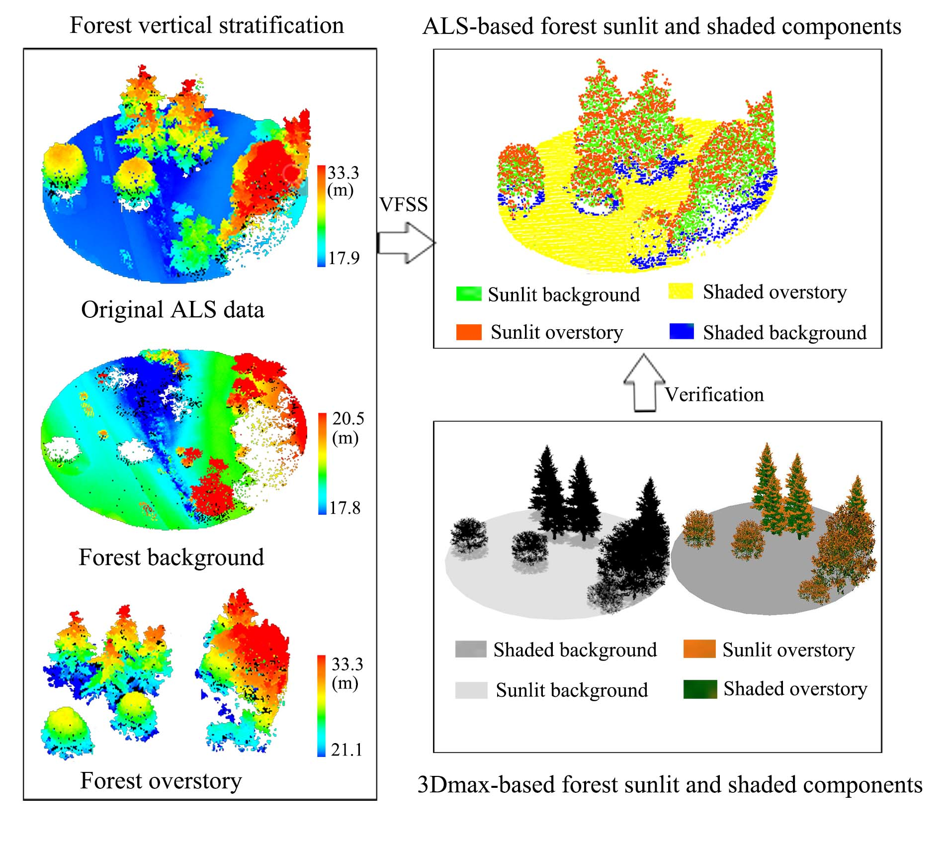
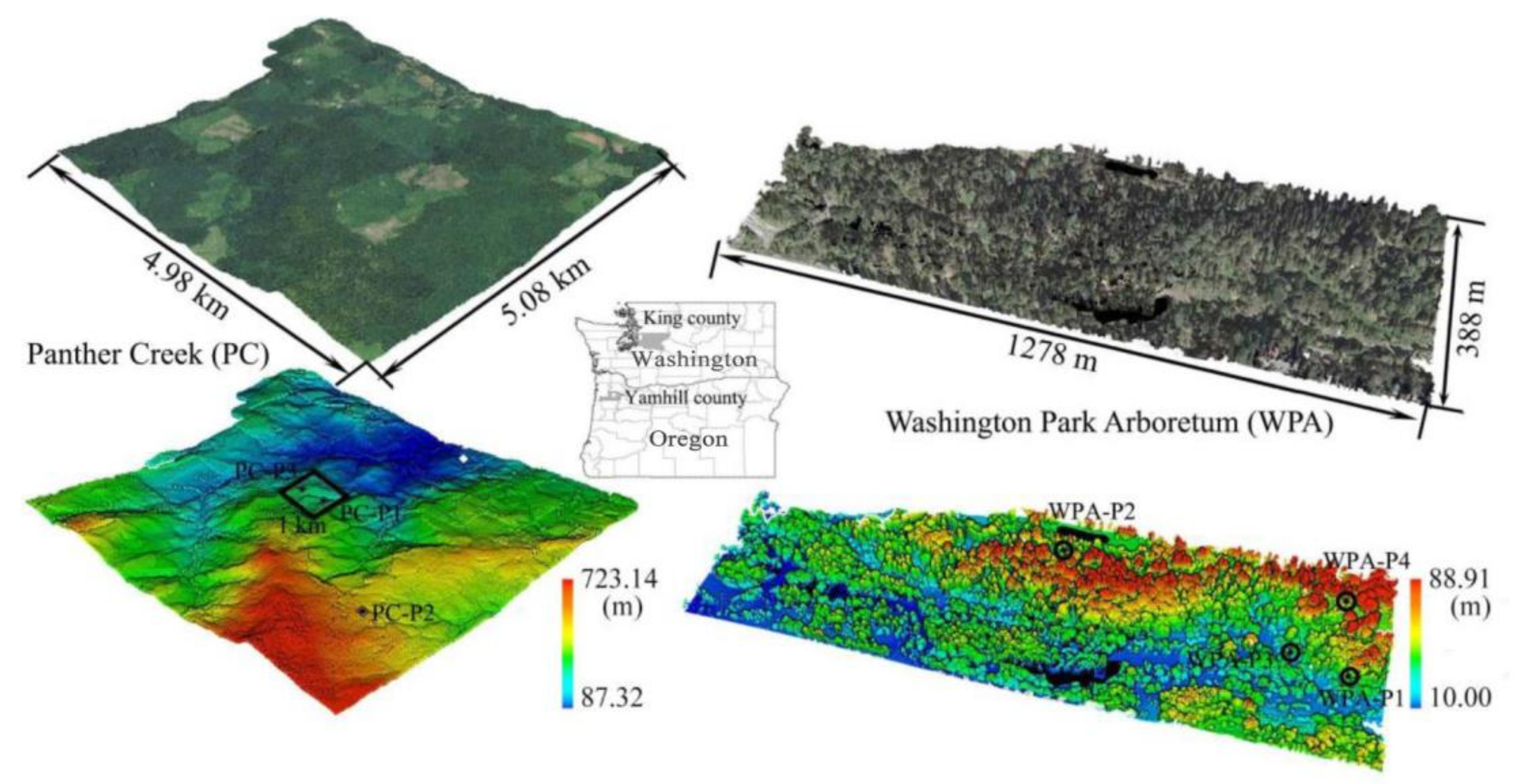
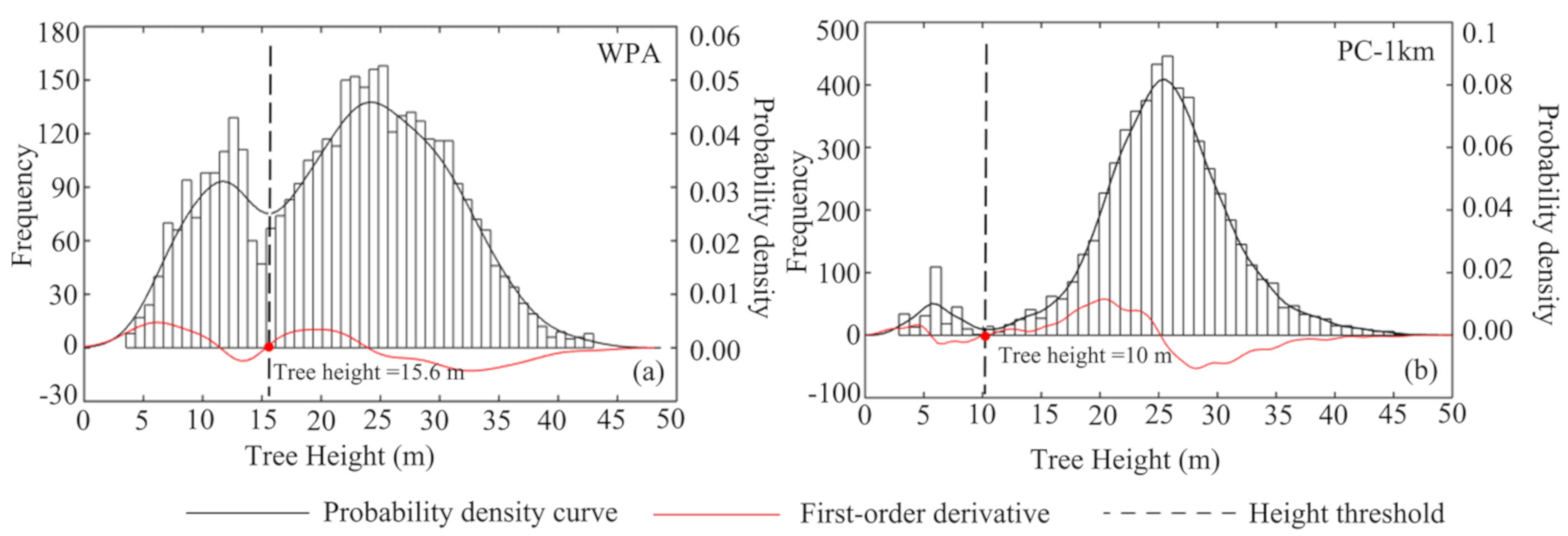
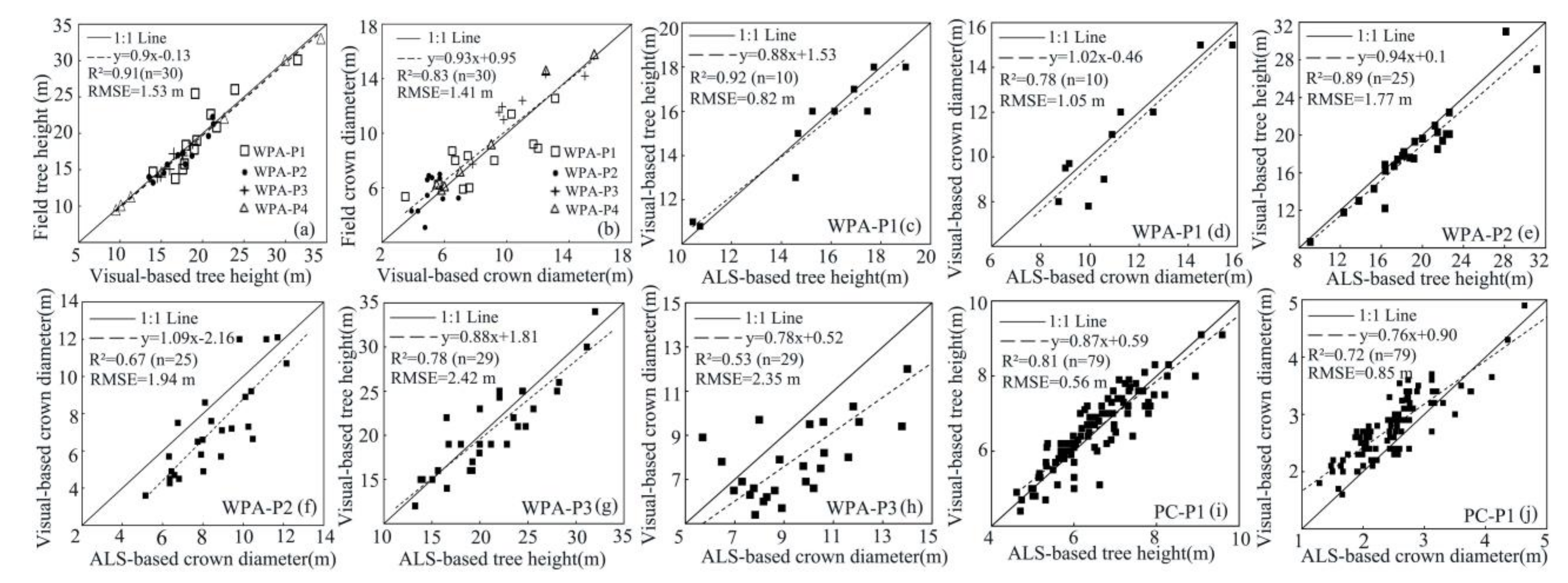
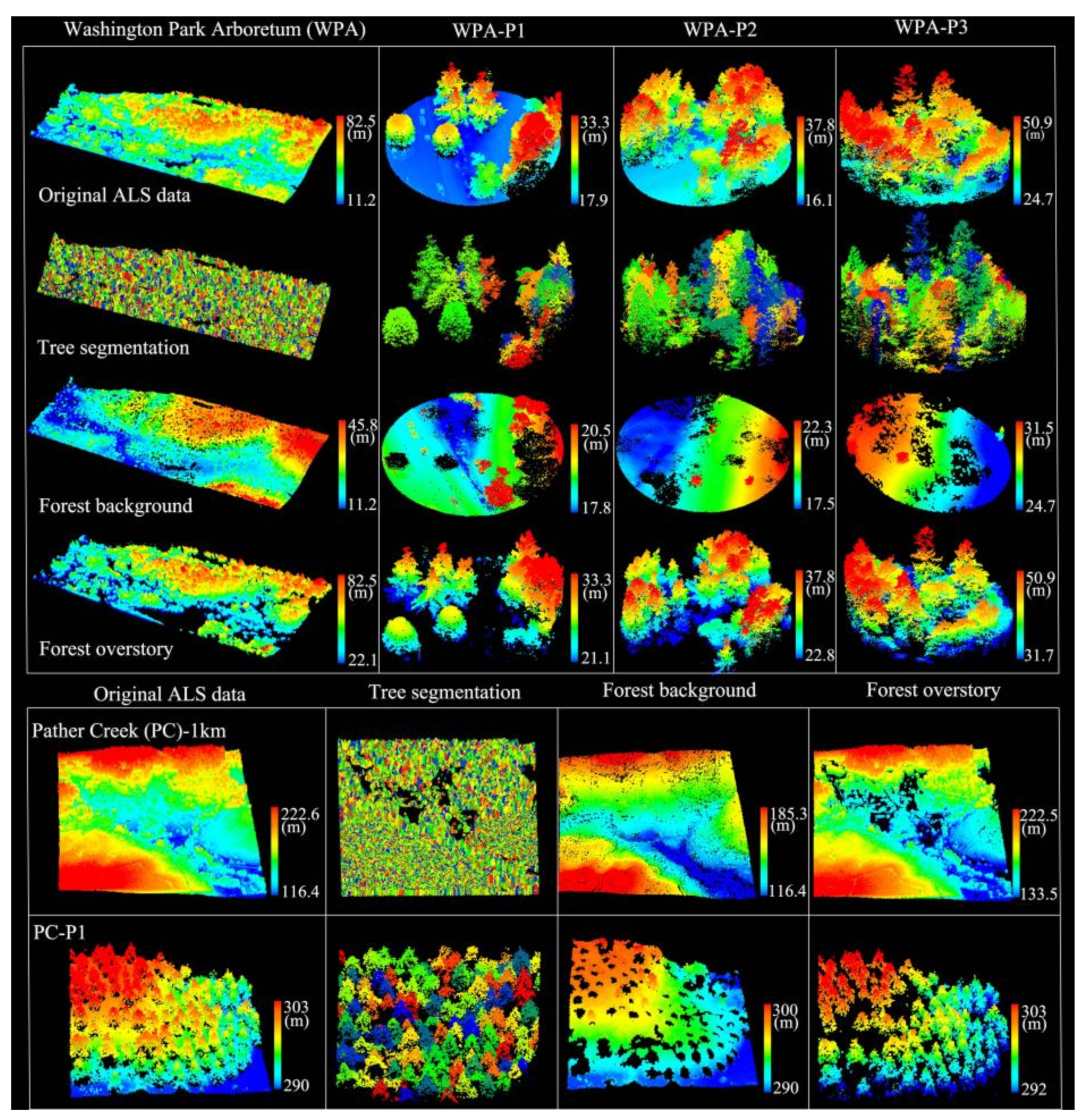
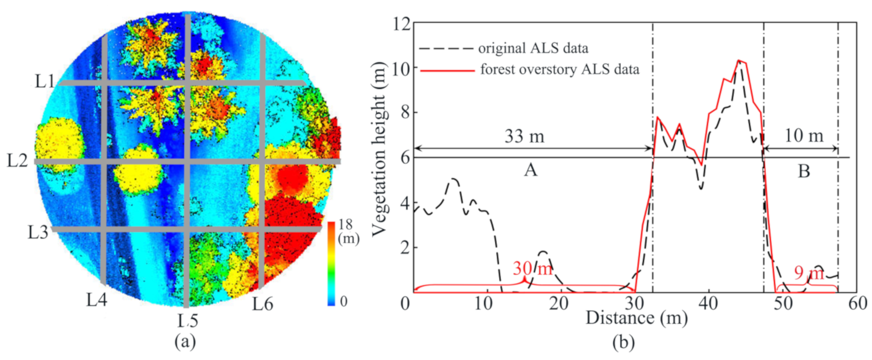
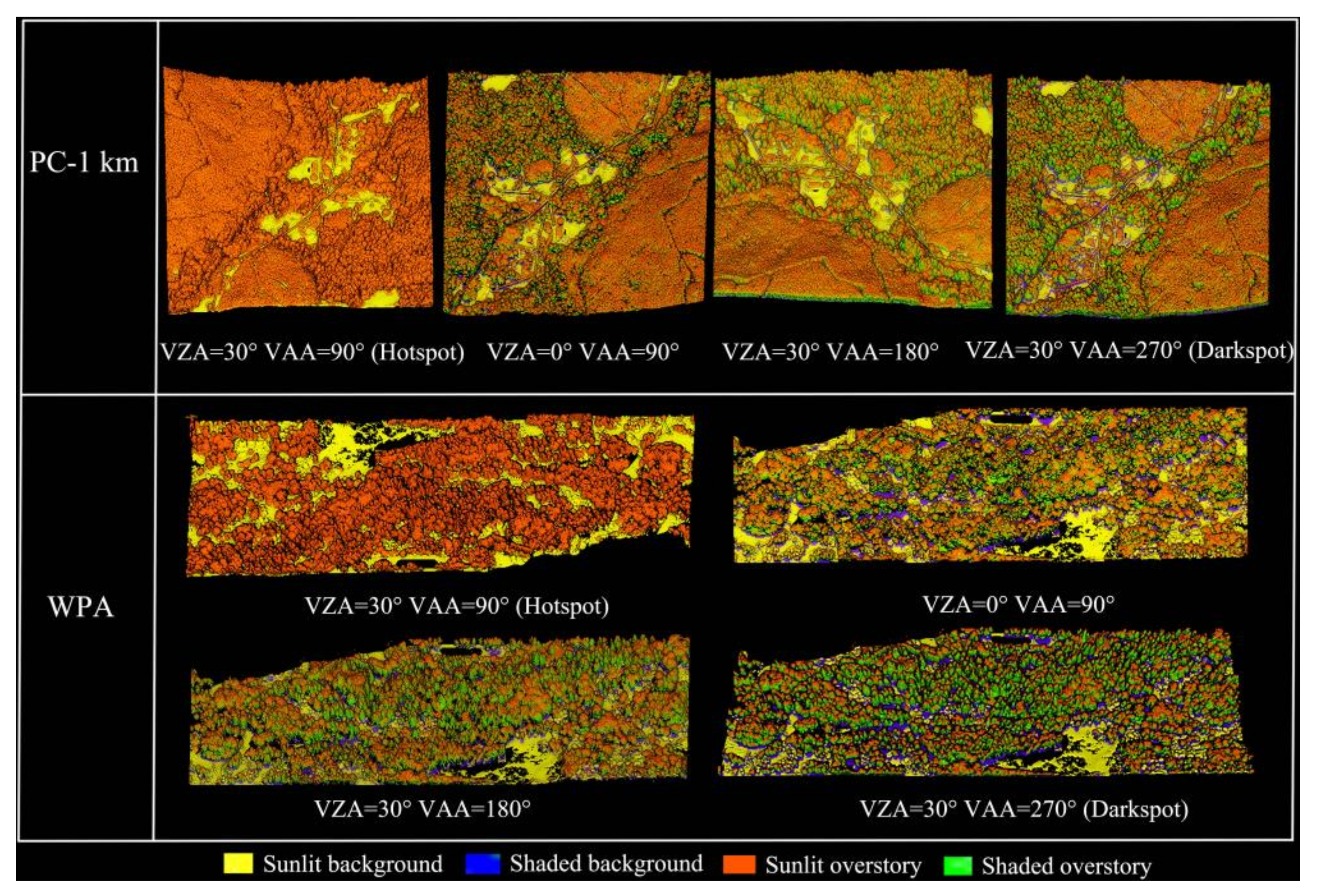
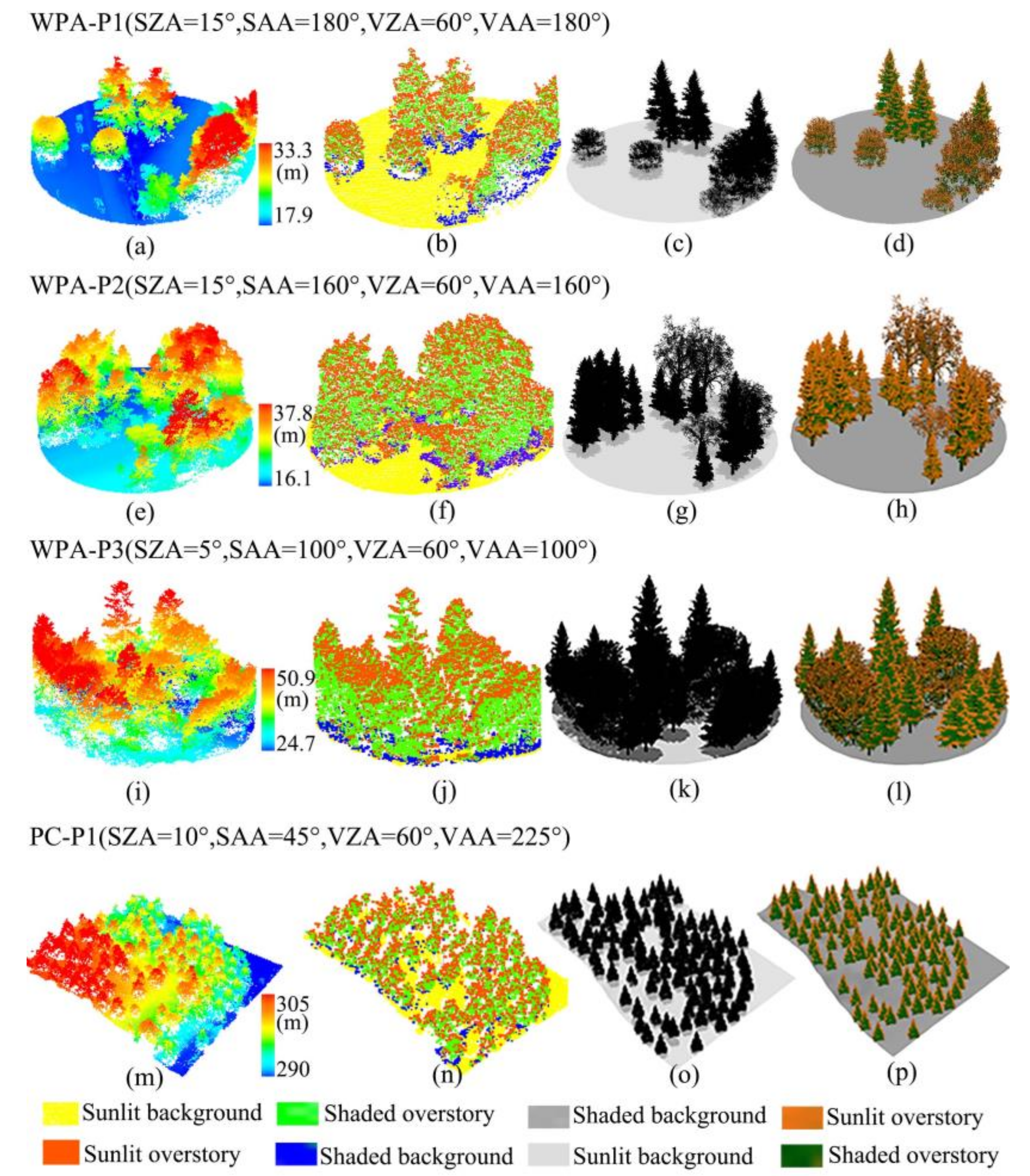
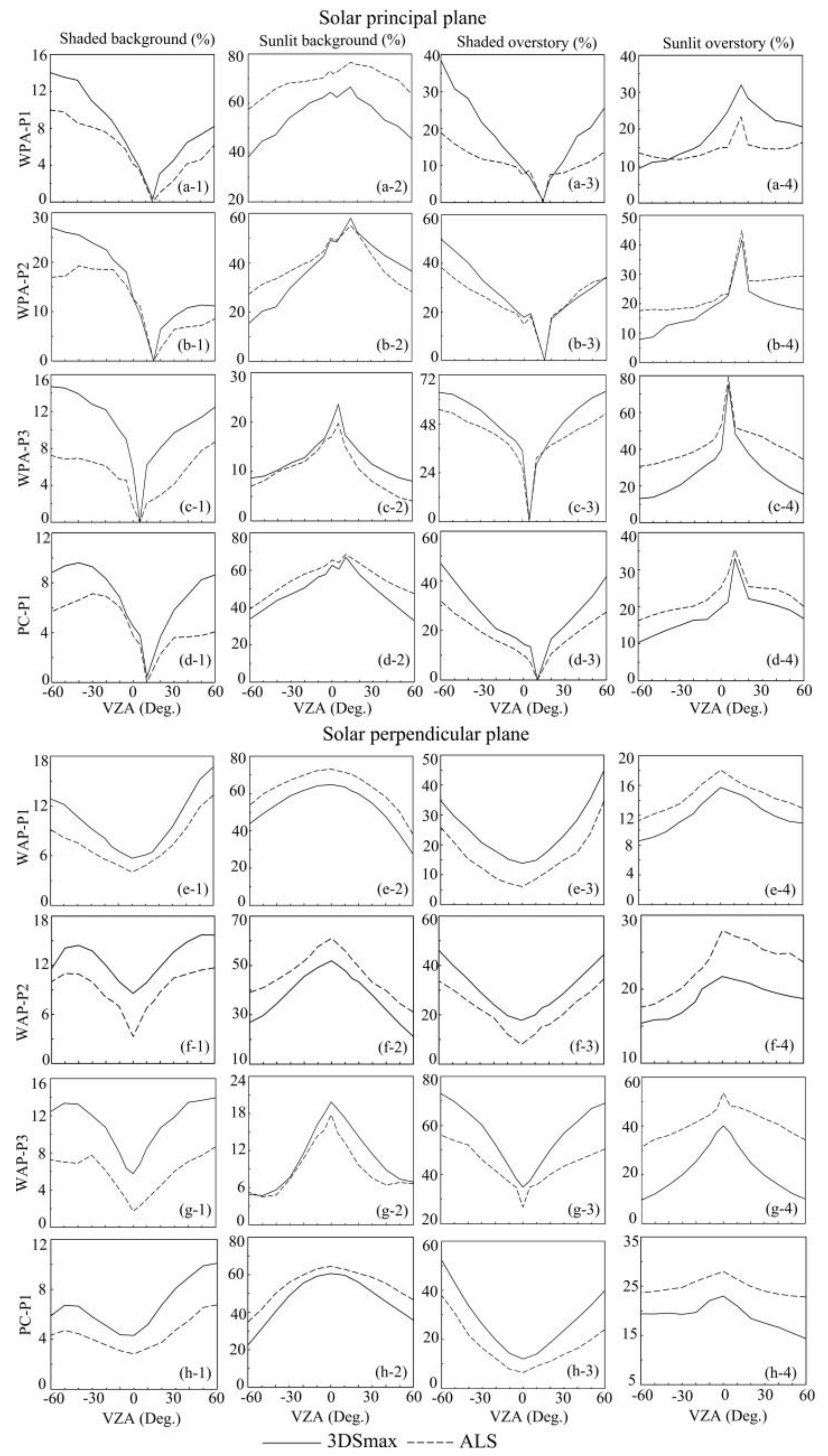
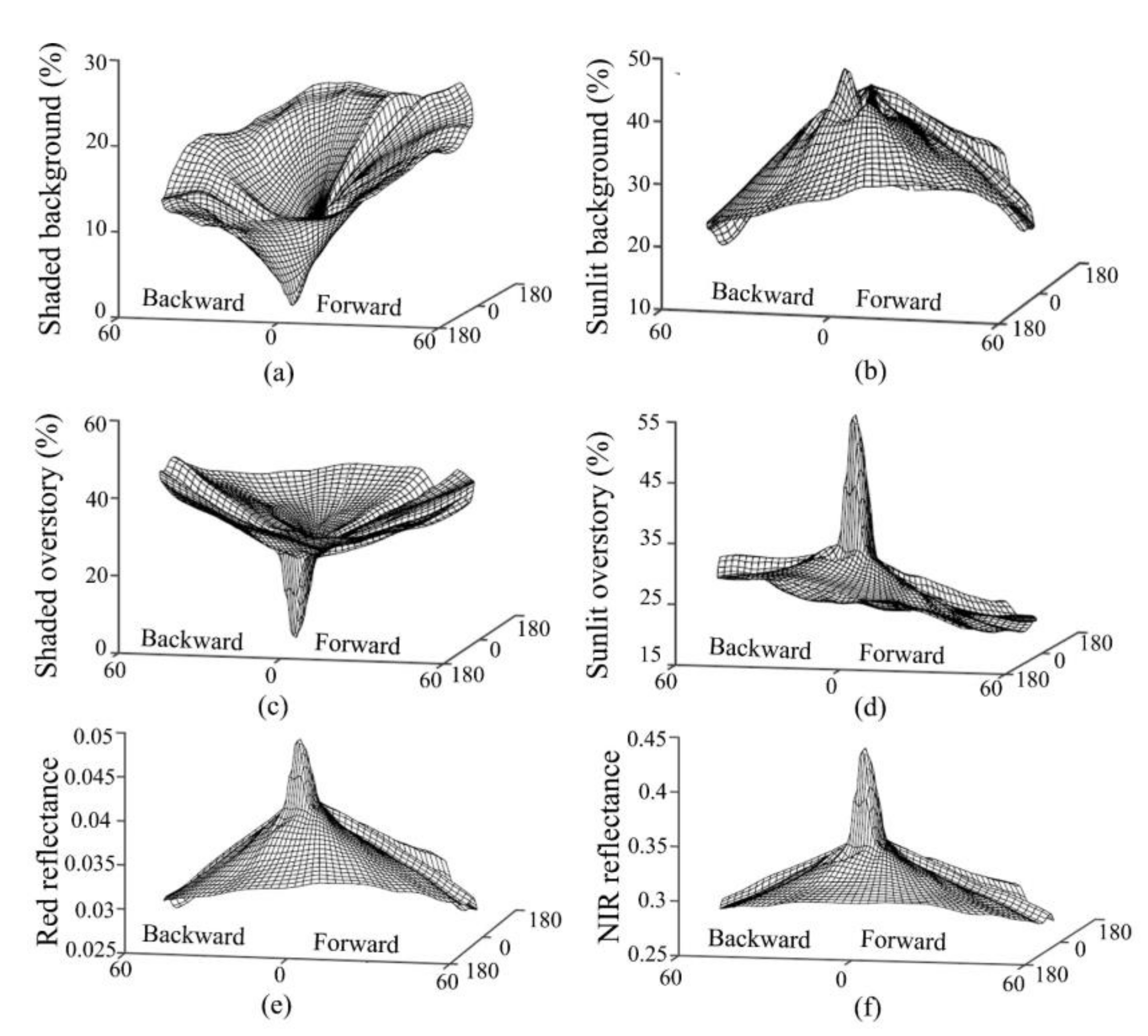
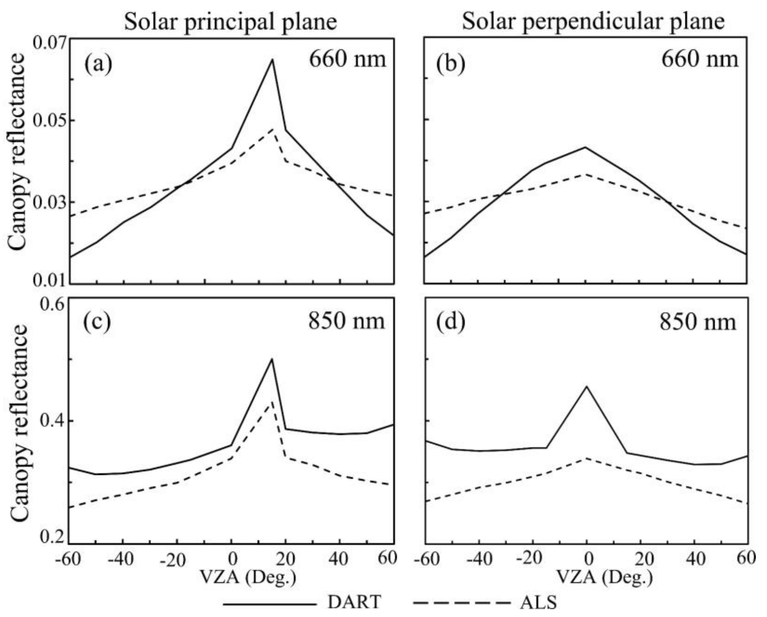
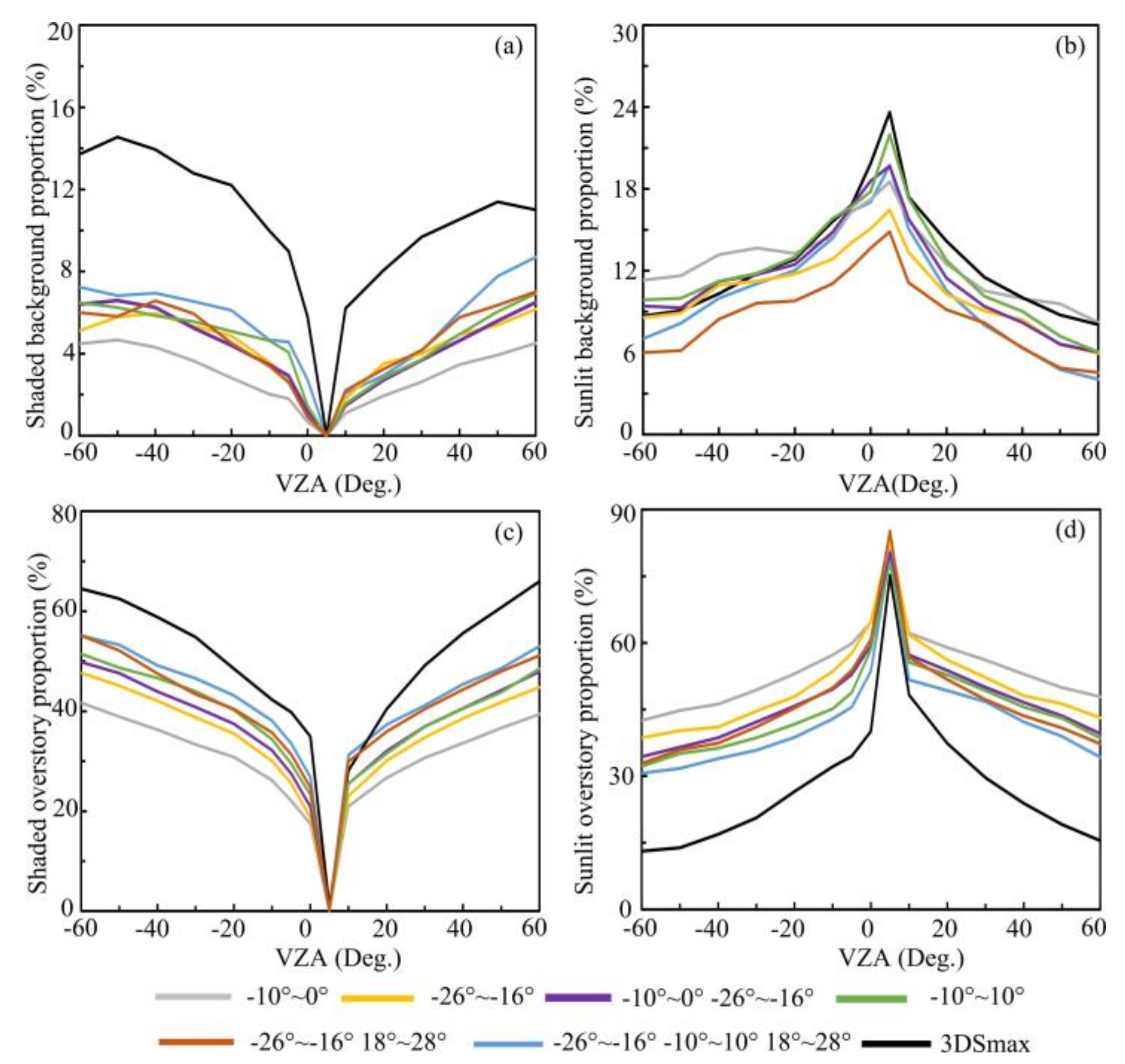
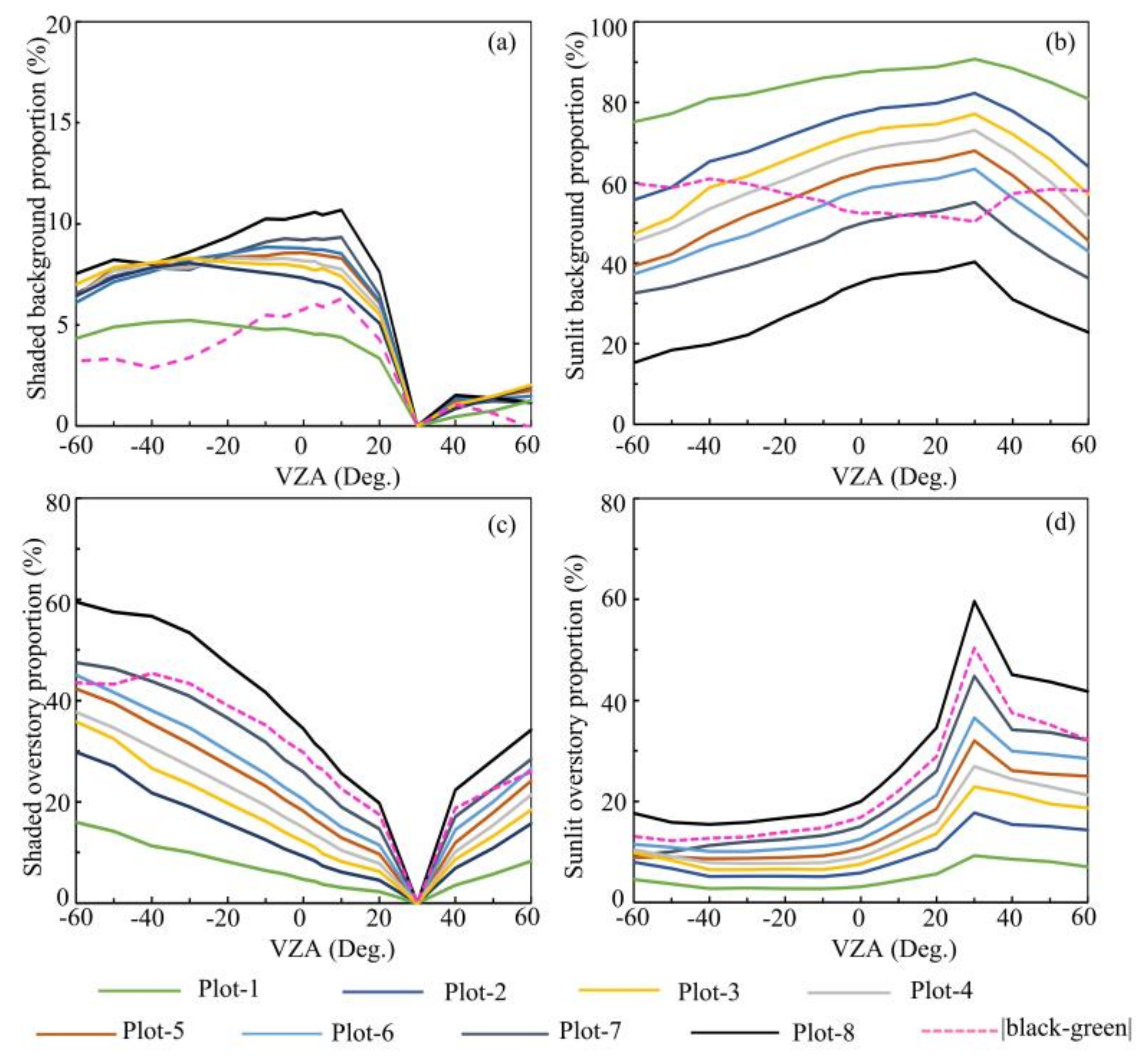
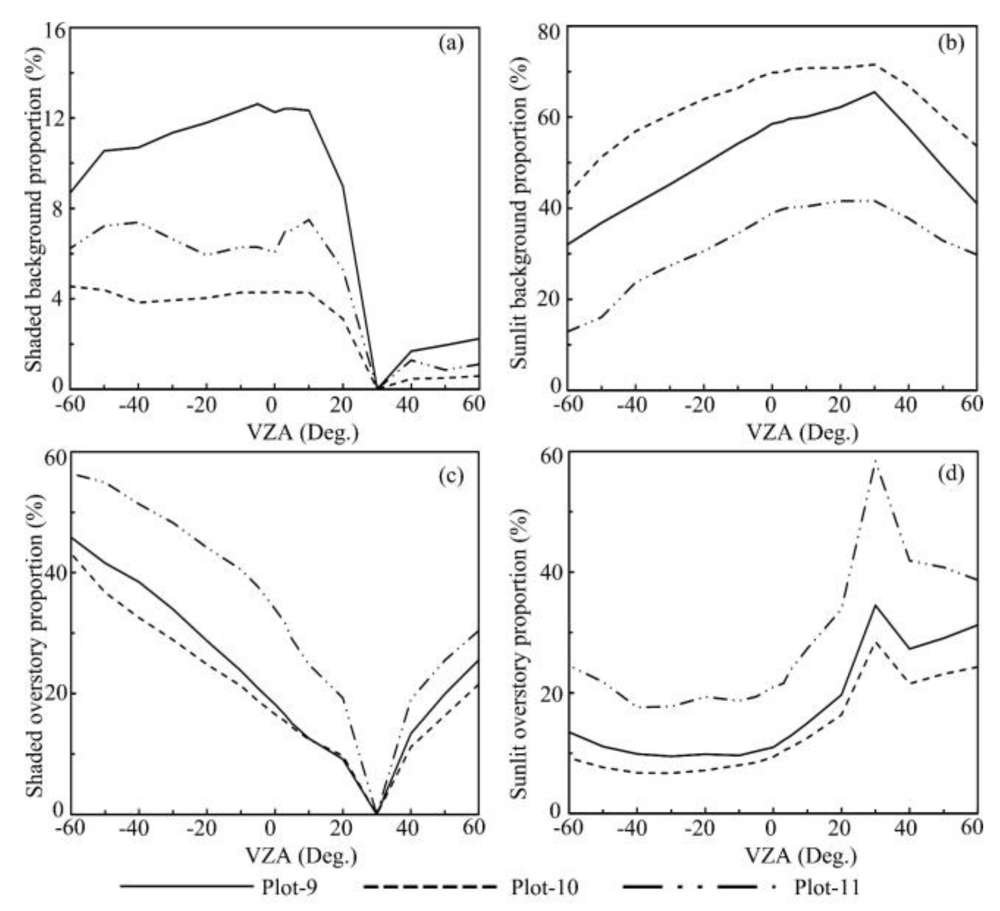
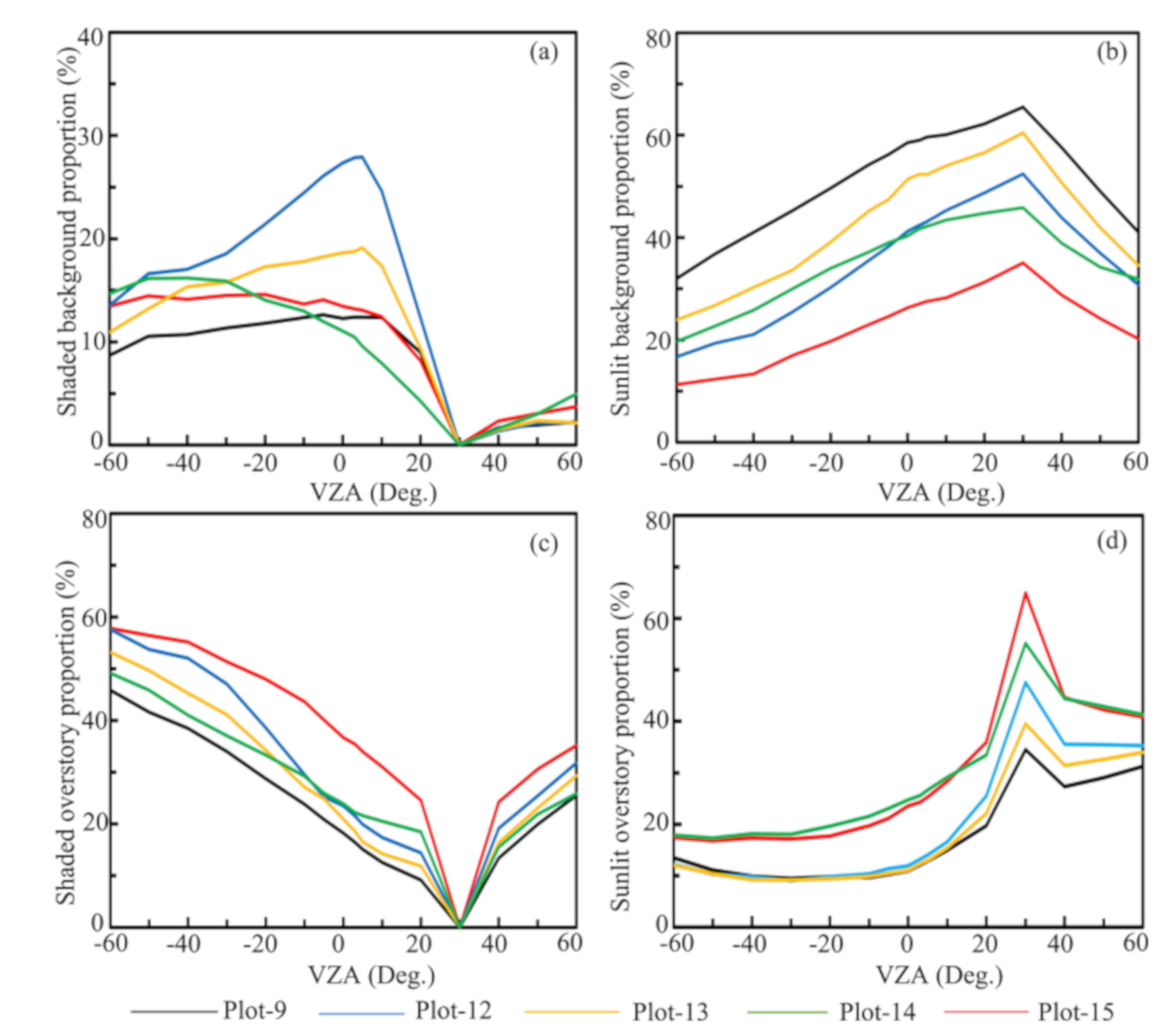
Table 1.
Characteristics of seven forest plots for forest plots in both Washington Park Arboretum (WPA) and Panther Creek (PC) sites.
Table 1.
Characteristics of seven forest plots for forest plots in both Washington Park Arboretum (WPA) and Panther Creek (PC) sites.
| Plot# | Forest Type | Density | Overpass Times | Number of Scan Angles | Scan Angle Range (°) | Tree Height (m) |
|---|---|---|---|---|---|---|
| WPA-P1 | Mixed | Low | 3 | 22 | -24 ~ -11, -8 ~ 0 | 6.0 -18.0 |
| WPA-P2 | Conifer | Medium | 2 | 32 | -29 ~ -7, -3 ~ 5 | 8.7 - 31.0 |
| WPA-P2E | Mixed | Medium | 5 | 57 | -29 ~ -7, -3 ~ 10, 18 ~ 28 | 3.7 - 25.4 |
| WPA-P3 | Mixed | High | 4 | 43 | -26 ~ -16, -10 ~ 10, 18 ~ 28 | 12.0 - 34.0 |
| WPA-P4 | Conifer | Medium | 1 | 13 | 7 ~ 19 | 13.0 - 27.0 |
| PC-P1 | Conifer | Low | 2 | 22 | -10 ~ -1, 2 ~ 12 | 4.5 - 9.8 |
| PC-P2 | Conifer | Medium | 2 | 24 | -8 ~ 5, -3 ~ 6 | 33.5 - 57.2 |
| PC-P3 | Conifer | Medium | 2 | 23 | -12 ~ -1, 3 ~ 13 | 18.6 - 38.8 |
Table 2.
Characteristics of 15 modeled forest plots based on aerial laser scanning data (ALS).
| Plot# | Tree Height (m) | Crown Diameter (m) | Stem No. | Canopy Cover (%) | Spatial Distribution Pattern | Crown Shape |
|---|---|---|---|---|---|---|
| 1 | 13 | 7.8 | 7 | 12 | regular | cone (conifer) |
| 2 | 13 | 7.8 | 14 | 23 | regular | cone (conifer) |
| 3 | 13 | 7.8 | 21 | 35 | regular | cone (conifer) |
| 4 | 13 | 7.8 | 28 | 46 | regular | cone (conifer) |
| 5 | 13 | 7.8 | 35 | 58 | regular | cone (conifer) |
| 6 | 13 | 7.8 | 43 | 71 | regular | cone (conifer) |
| 7 | 13 | 7.8 | 50 | 83 | regular | cone(conifer) |
| 8 | 13 | 7.8 | 56 | 93 | regular | cone(conifer) |
| 9 | 13 | 7.8 | 24 | 39 | regular | cone(conifer) |
| 10 | 13 | 7.8 | 42 | 37 | clumped | cone(conifer) |
| 11 | 13 | 7.8 | 42 | 71 | regular | cone(conifer) |
| 12 | 21 | 7.8 | 24 | 39 | regular | cone(conifer) |
| 13 | 21 / 13 | 7.8 | 24 | 39 | regular | cone(conifer) |
| 14 | 12 | 10.3 | 13 | 38 | regular | sphere(broadleaf) |
| 15 | 19 | 12.7 | 24 | 64 | regular | cone (conifer) |
Table 3.
Comparisons between the gap sizes obtained from stratified overstory and original ALS data and the root mean square errors of four forest component proportions between ALS and 3DSmax based in four forest plots (WPA-P1, WPA-P2, WPA-P3, and PC-P1).
Table 3.
Comparisons between the gap sizes obtained from stratified overstory and original ALS data and the root mean square errors of four forest component proportions between ALS and 3DSmax based in four forest plots (WPA-P1, WPA-P2, WPA-P3, and PC-P1).
| Plot# | WPA-P1 | WPA-P2 | WPA-P3 | PC-P1 | |
|---|---|---|---|---|---|
| Vertical stratification | Height threshold (m) | 6.0 | 6.9 | 5.4 | 3.5 |
| Original gap size (m) | 6.0 – 33.0 | 2.0 – 24.0 | 3.0 – 18.0 | 3.0 – 17.0 | |
| Overstorygap size (m) | 5.0 – 30.0 | 2.0- 22.0 | 1.0 – 13.0 | 3.0 – 15.0 | |
| Original gap size (m) | 137.0 | 179.0 | 114.0 | 144.0 | |
| Overstory gap size (m) | 116.0 | 143.0 | 64.0 | 125.0 | |
| Identification percentage (%) | 85.0 | 79.0 | 65.0 | 87.0 | |
| Gap size RMSE (m) | 2.3 | 2.7 | 4.3 | 1.8 | |
| Root mean square error (%) | Shaded background | 2.6 | 3.8 | 3.3 | 5.6 |
| Sunlit background | 12.1 | 7.0 | 2.7 | 9.8 | |
| Shaded overstory | 8.9 | 6.9 | 10.1 | 7.7 | |
| Sunlit overstory | 4.1 | 5.6 | 16.8 | 2.5 | |
| Forest background | 7.3 | 5.4 | 2.9 | 7.6 | |
| Forest overstory | 6.5 | 6.3 | 13.5 | 5.1 | |
| Background and overstory | 6.9 | 5.8 | 8.2 | 6.4 | |
Table 4.
Comparisons between the gap sizes obtained from stratified overstory and original ALS data and the root mean square errors of four forest component proportions between ALS- and 3DSmax-based in three forest plots (WPA-P4, PC-P2, and PC-P3).
Table 4.
Comparisons between the gap sizes obtained from stratified overstory and original ALS data and the root mean square errors of four forest component proportions between ALS- and 3DSmax-based in three forest plots (WPA-P4, PC-P2, and PC-P3).
| Plot# | WPA-P4 | PC-P2 | PC-P3 | |
|---|---|---|---|---|
| Vertical stratification | Height threshold (m) | 6.4 | 3.2 | 2.5 |
| Original gap size (m) | 5.0 – 17.0 | 3.0 – 10.0 | 3.0 – 9.0 | |
| Overstory gap size (m) | 4.0 – 16.0 | 1.0 – 7.0 | 1.0 – 6.0 | |
| Original gap size (m) | 143.0 | 75.0 | 53.0 | |
| Overstory gap size (m) | 102.0 | 56.0 | 36.0 | |
| Identification percentage (%) | 71.0 | 72.0 | 68.0 | |
| Gap size RMSE (m) | 3.9 | 2.5 | 2.9 | |
| Root mean square error (%) | Shaded background | 5.6 | 5.9 | 4.7 |
| Sunlit background | 9.7 | 8.1 | 8.9 | |
| Shaded overstory | 15.1 | 7.5 | 15.9 | |
| Sunlit overstory | 11.1 | 7.2 | 14.7 | |
| Forest background | 7.6 | 6.9 | 6.8 | |
| Forest overstory | 13.1 | 7.3 | 15.3 | |
| Background and overstory | 10.3 | 7.2 | 11.1 | |
Table 5.
Root mean square error of four forest component proportions between ALS- and 3DSmax-based results under different scan angles in WPA-P3.
Table 5.
Root mean square error of four forest component proportions between ALS- and 3DSmax-based results under different scan angles in WPA-P3.
| Root Mean Square Error (%) | |||||||
|---|---|---|---|---|---|---|---|
| Scan Angles (°) | Shaded Background | Sunlit Background | Shaded Overstory | Sunlit Overstory | Forest Background | Forest Overstory | Background and Overstory |
| -10° ~ 0° | 7.5 | 2.1 | 19.3 | 26.2 | 4.8 | 22.8 | 13.8 |
| -26° ~ -16° | 6.2 | 3.1 | 14.9 | 22.8 | 4.7 | 18.9 | 11.8 |
| -10° ~ 0° -26° ~ -16° | 6.2 | 2.7 | 12.9 | 19.6 | 4.5 | 16.2 | 10.4 |
| -10° ~ 10° | 5.9 | 1.3 | 11.2 | 17.3 | 3.6 | 14.3 | 9.0 |
| -26° ~ -16° 18° ~ 28° | 5.9 | 4.5 | 9.5 | 18.6 | 5.3 | 14.1 | 9.7 |
| -10° ~ 10° -26° ~ -16° 18° ~ 28° | 5.1 | 2.7 | 8.1 | 14.7 | 3.9 | 11.4 | 7.7 |
Table 6.
The comparison of four forest component proportions resulting from WPA-P2 and WPA-P2E plots.
Table 6.
The comparison of four forest component proportions resulting from WPA-P2 and WPA-P2E plots.
| Plane | View Azimuth Angle (°) | View Zenith Angle (°) | Four Forest Component Proportions Difference (%) | ||||
|---|---|---|---|---|---|---|---|
| Shaded Background | Sunlit Background | Shaded Overstory | Sunlit Overstory | Background and Overstory | |||
| Principal plane | 160 | 0 | 2.6 | 2.2 | 7.9 | 3.1 | 3.9 |
| 160 | 15* | 0.0 | 3.2 | 0.0 | 3.2 | 3.2 | |
| 160 | 20 | 0.1 | 2.7 | 11.8 | 8.9 | 5.9 | |
| 160 | 30 | 1.5 | 2.2 | 10.6 | 9.9 | 6.1 | |
| 160 | 40 | 4.8 | 4.9 | 11.7 | 11.6 | 8.3 | |
| 160 | 50 | 6.0 | 2.1 | 10.1 | 14.0 | 8.1 | |
| 160 | 60 | 6.5 | 12.3 | 4.6 | 23.4 | 11.7 | |
| 340 | 15 | 1.4 | 4.8 | 9.6 | 3.4 | 4.8 | |
| 340 | 20 | 0.7 | 4.2 | 8.5 | 4.7 | 4.5 | |
| 340 | 30 | 0.4 | 2.9 | 7.8 | 5.3 | 4.1 | |
| 340 | 40 | 2.1 | 0.9 | 6.2 | 7.4 | 4.2 | |
| 340 | 50 | 6.5 | 1.5 | 2.9 | 10.9 | 5.5 | |
| 340 | 60 | 13.7 | 8.3 | 3.7 | 18.5 | 11.0 | |
| Perpendicular plane | 70 | 15 | 0.0 | 5.9 | 11.3 | 5.4 | 5.7 |
| 70 | 20 | 0.4 | 6.1 | 11.3 | 5.5 | 5.8 | |
| 70 | 30 | 3.5 | 8.9 | 11.4 | 6.0 | 7.5 | |
| 70 | 40 | 6.9 | 8.6 | 10.6 | 8.8 | 8.7 | |
| 70 | 50 | 13.0 | 4.6 | 8.1 | 16.5 | 10.6 | |
| 70 | 60 | 14.4 | 1.2 | 8.1 | 23.6 | 11.8 | |
| 250 | 15 | 0.1 | 5.7 | 10.9 | 5.4 | 5.5 | |
| 250 | 20 | 1.1 | 6.8 | 10.6 | 4.9 | 5.8 | |
| 250 | 30 | 3.5 | 7.9 | 10.0 | 5.6 | 6.8 | |
| 250 | 40 | 4.6 | 7.5 | 8.7 | 5.8 | 6.6 | |
| 250 | 50 | 7.1 | 3.7 | 6.1 | 9.5 | 6.6 | |
| 250 | 60 | 7.3 | 3.2 | 3.3 | 13.8 | 6.9 | |
© 2020 by the authors. Licensee MDPI, Basel, Switzerland. This article is an open access article distributed under the terms and conditions of the Creative Commons Attribution (CC BY) license (http://creativecommons.org/licenses/by/4.0/).
Share and Cite
MDPI and ACS Style
Wang, X.; Zheng, G.; Yun, Z.; Xu, Z.; Moskal, L.M.; Tian, Q. Characterizing the Spatial Variations of Forest Sunlit and Shaded Components Using Discrete Aerial Lidar. Remote Sens. 2020, 12, 1071. https://doi.org/10.3390/rs12071071
AMA Style
Wang X, Zheng G, Yun Z, Xu Z, Moskal LM, Tian Q. Characterizing the Spatial Variations of Forest Sunlit and Shaded Components Using Discrete Aerial Lidar. Remote Sensing. 2020; 12(7):1071. https://doi.org/10.3390/rs12071071
Chicago/Turabian StyleWang, Xiaofei, Guang Zheng, Zengxin Yun, Zhaoshang Xu, L. Monika Moskal, and Qingjiu Tian. 2020. "Characterizing the Spatial Variations of Forest Sunlit and Shaded Components Using Discrete Aerial Lidar" Remote Sensing 12, no. 7: 1071. https://doi.org/10.3390/rs12071071
Note that from the first issue of 2016, this journal uses article numbers instead of page numbers. See further details here.