Estimation of Forest Growing Stock Volume with UAV Laser Scanning Data: Can It Be Done without Field Data?


Norwegian Institute for Bioeconomy Research (NIBIO), Division of Forest and Forest Resources, National Forest Inventory, Høgskoleveien 8, 1433 Ås, Norway
*
Author to whom correspondence should be addressed.
Remote Sens. 2020, 12(8), 1245; https://doi.org/10.3390/rs12081245
Submission received: 19 March 2020
/
Revised: 9 April 2020
/
Accepted: 13 April 2020
/
Published: 14 April 2020
(This article belongs to the Special Issue Lidar Remote Sensing of Forest Structure, Biomass and Dynamics)
Abstract
:Laser scanning data from unmanned aerial vehicles (UAV-LS) offer new opportunities to estimate forest growing stock volume () exclusively based on the UAV-LS data. We propose a method to measure tree attributes and using these measurements to estimate without the use of field data for calibration. The method consists of five steps: i) Using UAV-LS data, tree crowns are automatically identified and segmented wall-to-wall. ii) From all detected tree crowns, a sample is taken where diameter at breast height (DBH) can be recorded reliably as determined by visual assessment in the UAV-LS data. iii) Another sample of crowns is taken where tree species were identifiable from UAV image data. iv) DBH and tree species models are fit using the samples and applied to all detected tree crowns. v) Single tree volumes are predicted with existing allometric models using predicted species and DBH, and height directly obtained from UAV-LS. The method was applied to a Riegl-VUX data set with an average density of 1130 points m−2 and 3 cm orthomosaic acquired over an 8.8 ha managed boreal forest. The volumes of the identified trees were aggregated to estimate plot-, stand-, and forest-level volumes which were validated using 58 independently measured field plots. The root-mean-square deviance () decreased when increasing the spatial scale from the plot (32.2%) to stand (27.1%) and forest level (3.5%). The accuracy of the UAV-LS estimates varied given forest structure and was highest in open pine stands and lowest in dense birch or spruce stands. On the forest level, the estimates based on UAV-LS data were well within the 95% confidence interval of the intense field survey estimate, and both estimates had a similar precision. While the results are encouraging for further use of UAV-LS in the context of fully airborne forest inventories, future studies should confirm our findings in a variety of forest types and conditions.

1. Introduction
Forest growing stock volume (; m3 ha−1) is an essential measure used to characterise forest structure, value and is often used to estimate forest above-ground biomass (AGB; t ha−1). Maps and estimates of forest and its changes are central to understand the carbon and water cycles, for assessing the climate change mitigation potential of forests and to quantify ecosystem services [1]. Several earth observation missions, such as Global Ecosystem Dynamics Investigation (GEDI),
NASA-ISRO SAR Mission (NISAR), and BIOMASS, aim specifically at mapping forest AGB and will improve our ability to consistently map and estimate forest resources across the globe [2,3]. Still, all operational applications of remote sensing techniques for forest inventory require field observations for calibration of models and their validation [4]. Due to high costs of field work, the development of methods for forest inventories and mapping that only utilise remotely sensed data without the need for in-situ field data represent a breakthrough for the utility of RS data [5]. We will use the term ‘direct estimation’ to describe remote-sensing based estimates that are obtained without the use of in-situ field data for fitting or calibrating empirical models.
In the past decade, terrestrial laser scanning (TLS) emerged as a promising data source for directly estimating forest AGB [6,7,8]. Furthermore, airborne laser scanning (ALS) data have also been used to directly estimate AGB [5]. Recent technical development in miniaturised survey-grade laser scanning sensors suitable for unmanned aerial vehicles (UAV-LS) allows for the collection of detailed three-dimensional (3D) data similar to TLS data with the wall-to-wall characteristics of airborne data. Thanks to the combination of the wall-to-wall capabilities and the finely detailed representation of single trees, UAV-LS data opens new frontiers in direct forest measurement from remote sensing data [9].
UAV-LS data are particularly attractive as they allow for dense (1000–20,000 points m−2) sampling of the 3D structure of the forest canopy, including crowns, stems, branches, and understory vegetation. Thus, UAV-LS data have the potential to be used in a similar manner as TLS to obtain direct estimates of tree-level characteristics such as volume or AGB. While UAV-LS data have more occlusion than TLS data in the lower parts of the canopy, it can be collected on a much larger area and with only a fraction of the time for data acquisition. The possibility to use UAV-LS data for estimating AGB or growing stock is particularly attractive as calibration and validation datasets for space-borne earth observation programs [10]. In such applications, UAV-LS data may be used to estimate AGB or growing stock for the exact spatial extent and shape of the space-borne sensor footprint.
Early studies by Jaakkola et al. [11] and Wallace et al. [12] first introduced the use of UAV-LS for forest inventory. Since then, an increasing number of studies adopted single tree methods to assess biophysical properties such as tree height [13,14,15], tree crown properties [15,16,17], tree density [15], or diameter at breast height (DBH) measurements [14,18,19] and AGB [20,21]. The latter two variables are the most challenging and yet relevant, which potentially can justify the high costs of acquiring UAV-LS data. DBH is a relevant variable as it is widely used in forest inventory for valuation and simultaneously allows to obtain volumetric single tree estimates using existing allometric models. Despite the somewhat encouraging results in terms of DBH measurement accuracy (1–7 cm), the existing studies did not provide methods for how UAV-LS single tree measurements can be used to predict single tree volume. The exception is the recent study of Wang et al. [21] that adopted a tree-centric method [22] consisting of using measured height and DBH from UAV-LS data, with species information from a field-plot survey to predict single tree AGB using pre-existing allometric models. They obtained plot-level estimates by excluding the commission errors from the segmentation algorithm, which makes the method reliant on the availability of field data. A general finding of all UAV-LS studies is that DBH measurements are only possible for a sample of the entire population, including mainly dominant or isolated trees.
Based on the reported omission errors from UAV-LS data (15%–80%) and difficulties of measuring DBH for all trees [20,21], it is not foreseeable in the near future to obtain UAV-LS based AGB or growing stock predictions for all trees in a population. A key scientific challenge is, therefore, to develop methods for using the available UAV-LS single tree measurements into plot-, stand-, or forest-level estimates while accounting for the non-probability nature of the sampled trees.
Potential ways for direct estimation of AGB without the use of in-situ observations have been proposed [5,22,23,24] and consist of estimating single tree AGB by applying available allometric models using ALS-derived single tree variables (e.g., top height, crown area, crown base height) as predictors. While the approach developed by Ferraz et al. [5] is useful as it can be applied over large areas and can account for different vertical layers of the forest canopy, it was designed to segment tree crowns, and its applicability to discriminate between stems and understory vegetation in the lower parts of the canopy is unknown. The substantial increase in point density of UAV-LS data compared to ALS requires methods that, similar to TLS applications, can separate the stems from the other vegetation, especially in the lower parts of the canopy, thus allowing DBH measurements.
The objective of this study is to illustrate a model-based method to use a sample of trees with DBH, tree species and tree height measured from UAV-LS data to predict single tree and to use the predictions to estimate at the plot, stand, and forest levels. The proposed method relies solely on UAV-LS and field data (i.e., 58 plots) were used only for independent validation.
2. Materials
2.1. Study Area
The study area (59.65 N, 10.81 E) was located in south-eastern Norway and comprised 8.8 hectares of managed boreal forest. The study area has been subject to varying management and thus includes a variety of forest conditions in terms of forest cover, vertical distribution of the vegetation, and species composition. The vertical structure varied from single layer forests to multi-layered forests with continuous vegetation through the height profile. The forest cover varied from open single-story Scots pine (Pinus sylvestris L.) forests with low productivity (i.e., a minimum of 520 trees ha−1) to areas with full canopy cover (3440 trees ha−1) in highly productive Norway spruce (Picea abies (L.) Karst)-dominated stands. In most areas, the understory was characterised by a layer of birch (Betula pubescens and Betula pendula) ranging in height from 1 m to 5 m. Concerning the basal area, the dominant tree species were Scots pine (64% of the total), followed by Norway spruce (22%), and deciduous species (14%). In terms of tree density, according to the field data acquisition (see Section 2.2), the number of trees per hectare varied from a minimum of 400 to a maximum of 4400.
2.2. Field Data
Field data were acquired during 12 days in October 2017 by one field worker for a total cost of approximately 9900 Euros at the time of acquisition. The field data consisted of 58 systematically distributed field plots (Figure 1). The plots were located approximately on a 40 × 40 m grid. The systematic design was adopted in order to ensure a representative sample and a rather large sampling fraction. The field plots were circular and had a fixed area of 250 m2. The total area covered by the sample plots was approximately 1.5 hectares corresponding to a sampling fraction of 16.7% of the area of interest. This fraction was purposively large to estimate at stand and forest level with large precision and thus provide a suitable validation dataset.
The DBH (cm) and tree species were recorded for trees with DBH > 5 cm within each plot using the digital calliper DP II [25].Tree height (m) was measured for a subsample of 10 trees per plot using a Vertex Laser 5 [26]. The centre of each plot was measured using a Topcon GR-3 differential GPS [27].
For each plot, was predicted using the following procedure. The volume of each height sample tree was predicted using species-specific volume models [28,29,30] using DBH and height as predictor variables (see Annex 1 in Supplementary Materials for volume functions). The volume of the height sample trees was also predicted using the same models but with a predicted height according to standard height-DBH models [31,32]. The same models were also used to predict height and volume for trees with no height measurements. For the trees without height measurements, the volume was then adjusted by a plot and species-specific mean-of-ratios, calculated as the mean of the ratio of the volume of height sample trees using the true height and the predicted height. The plot-level volume was obtained as the sum of the individual trees’ volume within each plot scaled to per-hectare values. For the purpose of this study the area was manually delineated into 14 stands (Figure 1). The delineation was done according to tree species, canopy height and density from UAV-LS data. The stand area was on average 0.6 ha and in the range 0.2–1.1 ha. The forest level was defined as the union of all of the stands, or the entire area covered by the UAV-LS data. The stand- and forest-level volumes were estimated assuming simple random sampling using the plots available either within each stand or in the latter case using the entire set of field plots in the forest area. Summary statistics for the field data in terms of number of available observations, mean, minimum, and maximum are presented in Table 1.
2.3. Remotely Sensed Data
UAV-LS Data
UAV-LS data were acquired on 1 September 2017 by an external data provider for a cost of 10,500 Euros (costs inclusive of two UAV operators, equipment, licences, and data pre-processing). The data acquisition platform was a Camflight X8HL multirotor UAV [33] mounted with a Riegl-VUX-1 UAV laser scanning sensor [34] and Applanix AP 20 inertial navigation system and global navigation satellite system [35]. The data acquisition was conducted in two separate flights at 120 and 80 m above-ground level flown at 6 m sec−1. The total flight time was 37 minutes. The laser scanning sensor was configured to acquire data for with a scan angle ±45° from the nadir and to a measurement rate of 550 kHz. For both flights, perpendicular flight lines were flown (see Figure 1). The flight line spacing was equal to the flight altitude, thus ensuring an overlap between parallel flight lines of approximately 50%. Simultaneous to the UAV-LS data acquisition, a 24.3 megapixels SONY ILCE-6000 on-board camera acquired aerial imagery for the production of a 3 cm resolution orthomosaic and to colourise the point cloud. The weather conditions were optimal for UAV operations with wind speed < 1 m sec−1 and no cloud cover.
Pre-processing of the UAV-LS was performed by the contractor (Geomatikk AS) and included (1) calculation of the flight trajectory from inertial measurement unit; (2) computation of global x, y, and z coordinates from the trajectory and raw laser data using Riegl RiProcess [36]; (3) ground classification and flight line matching using Terrasolid Terrascan/Terramatch [37]; and (4) generation of a triangulated irregular network using the ground classified points to obtain relative tree heights above-ground. The reported standard deviation between the UAV-LS data and control surfaces placed in the area of interest before the UAV data acquisition was 1.95 cm, indicating a high level of geometrical accuracy. The UAV-LS data collected from 120 m and 80 m above ground were merged to obtain a point cloud with an average density of 1130 points m−2. A minimum = 594 points m−2 and a maximum = 1527 points m−2 were observed on the 58 validation plots. The two datasets were merged as the density of each separate acquisition was not deemed sufficient for DBH measurements. Figure 2 illustrates the point cloud from the Riegl VUX-1 to highlight the level of detail throughout the vertical canopy profile.
3. Methods
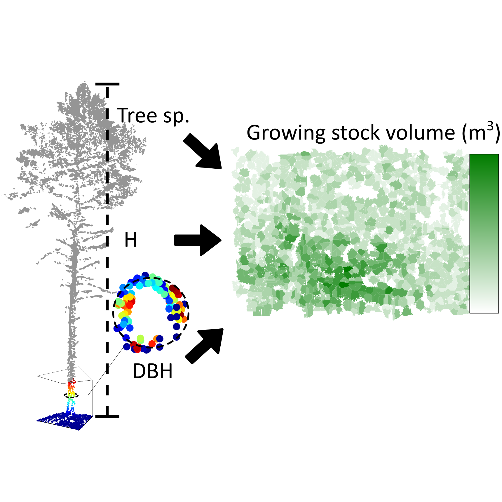
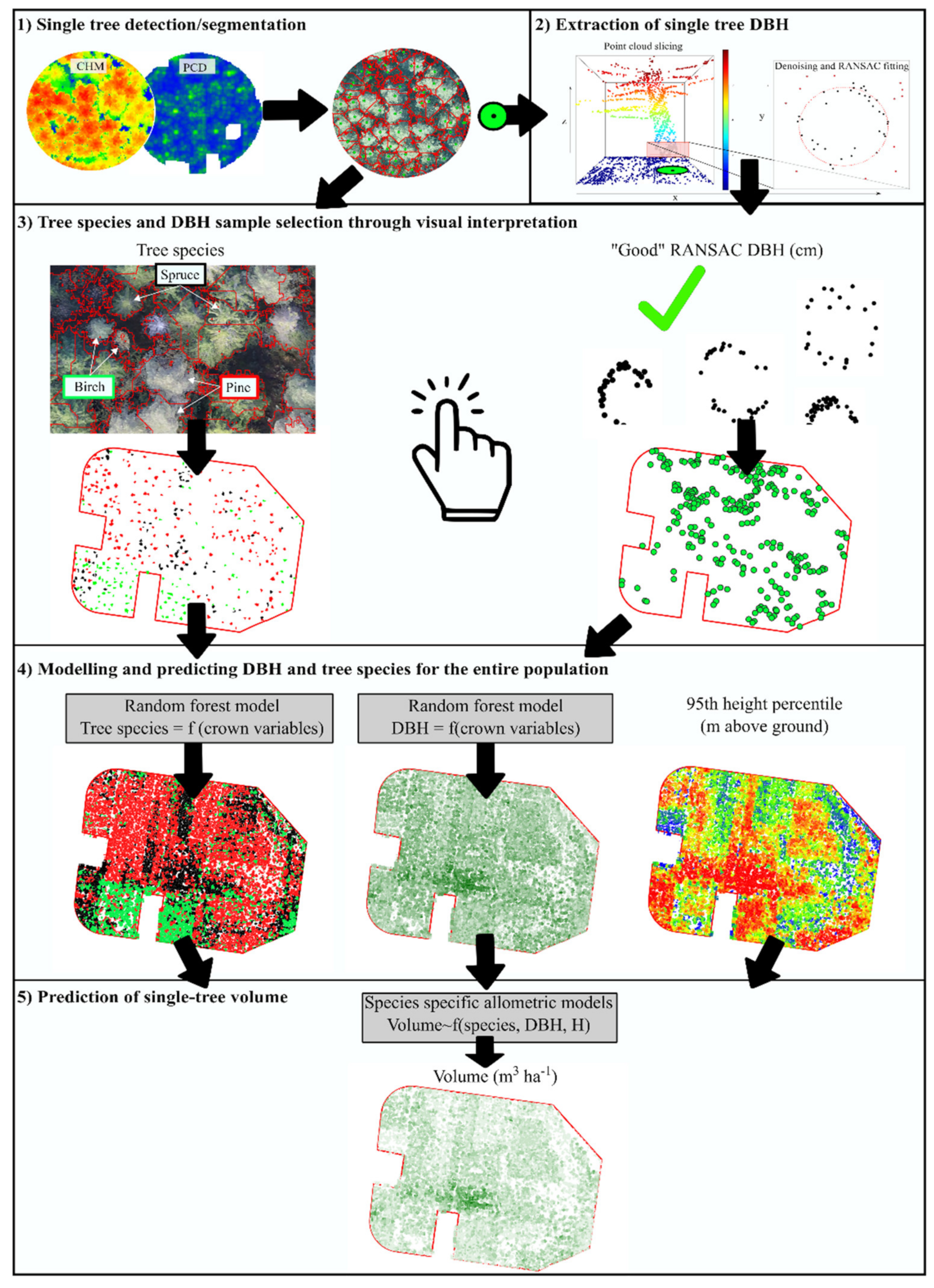
The proposed method consists of five steps (Figure 3): (1) single tree detection and segmentation, (2) manual selection of a sample of single tree DBH from the UAV-LS point cloud, (3) visual interpretation of a sample of crowns where tree species was identifiable from UAV data, (4) modelling and predicting DBH and tree species on all the detected tree crowns, and (5) prediction of single tree volume using existing species-specific allometric models using predicted DBH and UAV-LS derived height (i.e., 95th percentile of height values). The final output was the single tree (m3) directly estimated using UAV-LS data.
3.1. Step 1: Tree Detection and Segmentation
The detection and segmentation of single trees is step 1) in the proposed method (Figure 3). Prior to the detection of the single trees, two raster datasets were generated from the UAV-LS point cloud—namely, a canopy height model (CHM; pixels size = 0.1 m) and a horizontal point cloud density (PCD; pixels size = 0.2 m). The former was obtained by subtracting the digital terrain model (DTM) from a digital surface model (DSM), thus representing the top of the canopy. The resolution of the CHM was determined as the smallest pixel size without incurring in excessive no data values. While the selection of smaller pixel would not add relevant precision to the treetops’ locations, for sparse UAV-LS data, the pixel size may need to be increased based on the point density. The PCD is a raster of the percentage of returns within the cell in relation to the total number of returns in the study area. The PCD pixel size was twice of that of the CHM in order to reduce noise from isolated clusters of points. This type of raster product has been more often used in relation to TLS data [38,39,40]. However, with the capabilities of UAV-LS to retrieve stem returns, such raster products are also of interest for UAV-LS applications [14]. A local maxima approach was adopted for the location of single tree positions. This was implemented separately on the CHM (i.e., finding the treetops) and on the PCD (i.e., to find stems). The use of the latter was included to reduce typical omission errors caused by the missed detection of understory trees when using only the CHM. The window size for determining local maxima was set to 2 m × 2 m and 1 m × 1 m for the CHM and the PCD, respectively. The window size was determined by considering the minimum distance between two neighbouring treetops. In our case, 2 m × 2 m was a reasonably large to avoid detecting multiple treetops within a single crown (commission errors) while avoiding multiple trees being segmented as one (omission errors). The window size for the local maxima search was smaller for the PCD compared to the CHM because as the former includes data points from all trees and not only the dominant trees as in the CHM. Thus, assuming that the PCD describes a larger number of trees, it was justified to select a smaller window size. The positions of the detected trees using both raster layers were then merged by removing the duplicates (distance between two points < 0.5 m). This parameter describes the minimum distance between tree stems and was determined by a trial and error approach guided by the visualization of the detected trees in the point cloud.
A segmentation of the tree crowns corresponding to the detected trees was performed using the algorithm by Dalponte and Coomes [22] implemented in the R package lidR [41]. The parameters used were height threshold 2 m, threshold seed 0.3, threshold crown 0.4, and maximum crown diameter of 10 m. These parameters were selected after visual inspection of different settings on the detected tree crowns. For each tree crown, 93 explanatory variables were calculated from the UAV-LS point cloud, including height percentiles (, ,…,,); intensity percentiles (, ,…,); density variables (, ,…,); the slope () and intercept () of a linear regression line fitted to the density variables, crown geometry variables (projected crown area on a horizontal surface: , perimeter: , and their ratio: ); and spectral variables from the RGB values assigned to each point using the UAV orthomosaic such as band averages (, , ), standard deviations (, , ) and their ratios (, , ).
3.2. Step 2: Diameter Measurements
Step 2 that aims at individual tree diameter measurement consists of two processes including point clustering and circumference fitting for individual trees.
3.2.1. Point Cloud Clustering
The point cloud data were sliced for a height interval ranging between 0.8 m and 1.8 m. The returns within this slice included both stems as well noise from the understory vegetation and low branches. Noise removal was performed separately for each detected tree in Step 1 within a buffer of size of 0.3 m around the tree position. The 0.3 m threshold was determined by selecting the radius that would correspond to an un-realistically large DBH value (60 cm) in the study area. An unsupervised k-means clustering with k = 2 was used to discriminate between stem and noise returns. The covariates used in the k-means clustering were x, y coordinates, intensity, point density, average distance in the x, y, z space. The point density was defined as the PCD pixel value corresponding to each point’s location and was included in order to favour the removal of isolated points. The x, y and average x, y, z distances were computed as the row mean value of a distance matrix including all the points within the stem buffer using either only the x, y coordinates or including also the z values. These two variables were used to discriminate between clusters of scattered points (noise) and clusters of nearby points in the x, y, and z space (likely stems). Out of the two resulting clusters, the one with the smallest average x, y, z distance was selected as the stem.
3.2.2. Circumference Fitting
Based on the selected stem cluster, the DBH was estimated from circumferences fitted using the random sample consensus (RANSAC) algorithm implemented in the TreeLS R package [42]. The input to the algorithm is a matrix with x, y, and z coordinates for each detected tree. The remaining parameters are the length of stem segments to fit (; m), number of points to sample in each iteration (), the proportion of inlier points (), and the level of confidence desired (). In this study, we adopted equal to the height of the point cloud slice (1 m) extracted for DBH measurement. The value was dependent of the number of stem-classified points available in the 1 m vertical slice and was 10 for trees with more than 20 points and 50% of the number of points when these were less than 20 points. The proportion of inliers was set to = 0.7 as, after the previous denoising step, most points were assumed to be from the stem. Also, the confidence level value was set to a very high value (= 0.99) to ensure the selection of the best quality DBH measurements. These parameters were determined by a visualization of the fitted circumferences superimposed on the horizontal distribution of the stem points (see Figure 4).
3.3. Step 3: DBH and Tree Species Sample Selection
In Step 3 (Figure 3), we manually selected two separate samples of detected tree crowns—one sample with reliable DBH measurements and another sample with identifiable trees species. Out of all the trees with RANSAC measurements, we selected a sample (n = 305) of reliable DBH measurements by visual interpretation of the RANSAC inlier points. The reliability of DBH measurements was determined by the comparison between RANSAC measurements and diameter measured manually on the point cloud in a GIS environment (Figure 4). The manual selection of trees was performed with particular attention to:
- -
- Reduce the DBH measurement error, i.e., trees with little UAV-LS data occlusion and absence of branches at breast height (±1 m), with returns distributed in cylindrical shapes;
- -
- Include much of the variability in the study area, i.e., trees distributed across a wide range of DBH (5–50 cm), tree species, and geographically distributed throughout the area.
The second sample, consisting of tree crowns with associated tree species information, was collected through visual photo interpretation of a very high resolution (3 cm) orthomosaic (Figure 4) produced from the RGB images acquired simultaneously to the UAV-LS data. For a total of 393 detected tree crowns, the tree species could be easily identified as either spruce, pine, or deciduous. The sampling fraction of the DBH and tree species samples based on the total number of detected trees were 3.2% and 4.1%, respectively. The whole process of visually selecting the abovementioned samples required approximately four hours.
3.4. Step 4: Modelling and Predicting Tree DBH and Species
In Step 4 (Figure 3), the two samples described in the previous section were used to develop two separate Random Forests models [43] for DBH and tree species. The UAV-LS metrics calculated for each crown (Section 3.1) were used as explanatory variables. The default parameter settings for the Random Forest function [44] were used, i.e., the number of trees was 500, and number of variables randomly sampled as candidates at each split was equal to for the tree species classification and for the DBH regression models respectively, where was equal to the number of predictor variables. We selected as predictor variables only the 10 most important variables according to node purity for the DBH model and mean decreased Gini coefficient for the tree species model. The number of 10 variables was arbitrarily selected to avoid including too many variables. The models were then applied to the entire set of detected tree crowns to predict DBH and tree species.
3.5. Step 5: Predicting Volume for All Detected Trees
In Step 5 (Figure 3), for each tree crown the single tree predictions of tree species, DBH, and UAV-LS measured tree height (i.e., 95 height percentile) were used as predictors in the allometric models described in Section 2.2 (see Annex 1 in Supplementary Materials) to predict the single tree volume (m3).
The single-tree volume was then aggregated to plot, stand, and forest levels by summing up all of the single-tree values and dividing by the area to obtain per hectare values.
3.6. Validation
At plot, stand, and forest levels, the following statistics were used to compare the UAV-based estimates with the field data. The root-mean-square deviance () and mean difference () were calculated on all (plot, stand, and forest) levels. The term is used rather than root-mean-square error because estimates based on field data rather than true observations are compared to UAV-LS estimates on stand and forest level.
where is either the number of plots, the number of plots within a stand, or one. In the latter case, i.e., on the forest level, the is the absolute difference between the forest level estimate of the mean based on field plots and the forest level estimate based on UAV-LS. symbolises mean volume per hectare at the plot, stand, or forest level based on field data. symbolizes the mean volume per hectare at the plot, stand, or forest level based on UAV-LS data. Formally, are synthetic estimates [45] and fully rely on the fitted models for DBH and species.
Due to the lack of single tree positions in the field data, the detected trees could not be matched with field measured trees, and thus the validation on segment level was not possible.
We compared the with the uncertainty of the field data for estimating on the respective level. The standard deviation is the square root of the sample variance ():
where is the mean of the field-based observations on the respective levels. While the was used at the plot level, the standard error () was used for the stand and forest level:
In order to provide an estimate of the uncertainty of the UAV-LS estimates at the plot, stand, and forest levels, we adopted a non-parametric bootstrapping approach [46] to estimate the variance. Considering of total number of = 1000 iterations, at the 𝑏th iteration we i) selected a simple random sample with replacement of equal size to that of the original sets of data (i.e., sets for modelling either DBH and tree species), (ii) re-fit and predict volumes for all detected trees (Steps 4 and 5 in Figure 3), and iii) estimate the mean () for each level (plot, stand, or forest). Finally, we estimated the bootstrapping mean and variance according to
The standard error of the bootstrap estimates () was then calculated as the square root of for the plot, stand, and forest levels.
The distribution of absolute differences on plot level given dominant species, species mix, and, stem density were analysed to describe the influence of forest structure on the UAV-LS estimates.
4. Results
The results of the Random Forests model for the DBH model highlighted the importance of height percentiles, crown shape, and spectral variables to describe the DBH variation (Figure 5). For the tree species model, the most important variables were the spectral variables, followed by (i.e., the rate of decrease of point density when going from the ground level to the tree top), and two-point density variables corresponding to vertical slices taken at one-third of the total tree height (d30, d40).
The scatterplot of the DBH model’s predictions against the field measurements (Figure 6) revealed that despite a reasonably good model fit for the observations around the average, there was a tendency of over-predicting small DBH values and under-predicting large DBH values.
The accuracy assessment of the tree species model was performed by comparing out-of-bag predictions with observations (Table 2). The overall accuracy was 77.1% and the species-specific producer’s accuracy was 79.5%, 86.7%, and 57.8% for spruce, pine, and deciduous species. The poorer performance of the deciduous class was mainly described by the fact that 36% of the deciduous trees in the sample were classified as pine.
The plot-level validation was performed using = 58 field plots and the scatterplot of the UAV estimated against the field measured volume revealed a strong correlation between the two (Figure 7a). The was 103.4 m3 ha−1 or 32% of the mean, and despite the presence of two pine-dominated plots with large residuals, there were no substantial differences among the valuesby tree species (not shown). However, it was noteworthy that was underestimated for most of the spruce-dominated plots. The largest residuals were found for plots composed of a dominant layer of large pine trees and a co-dominant layer of spruce and birch. The bootstrap estimates revealed an average for the UAV-LS plot measurements across all plots of 31.5 m3 ha−1, corresponding to 9.7% of the mean value.
The stand-level validation was performed using = 14 stands. The scatterplot of the UAV stand estimates against the field estimated volume (Figure 7b) revealed that the averaging of plot or tree level values reduced the volume ranges and thus reduced the to 93.1 (= 28.9%). As for the plot-level validation, the was slightly underestimated for spruce-dominated stands while the same was not evident for the other tree species. It is, however, important to remember that for nearly 50% of the stands the uncertainty of the field estimates was rather large (see Figure 7) given that it was based on only three field plots for some stands. Furthermore, was of 26.0 m3 ha−1, or 7.6% of the mean on average.
The forest-level validation was performed by comparing the estimated mean based on the volume predictions for all UAV-detected tree crowns (n = 9111) with the design-based estimate using all field plots (n = 58). The mean volume from the UAV measurements was 3.5% larger than the field estimated mean volume (Table 3) but well within the 95% confidence interval of the design-based point estimate. Furthermore, the precision of the UAV estimate was similar (SE = 18.0 m3 ha−1) to the design-based estimate (SE = 18.6 m3 ha−1) (Figure 7).
The analysis of the plot-level absolute differences between the field measured and the UAV-LS estimated (Figure 8) revealed that the estimates were affected by tree density, dominant species, and species mix. The most accurate results were found for open (0–1000 trees ha−1) pine-dominated plots. The accuracy decreased with increasing tree density and was found to be smallest for deciduous-dominated plots. Concerning the effect of species mix on the accuracy of the predictions, we found larger accuracy in pure stands (i.e., stands where the for one of the tree species > 70% of total plot ) compared to mixed-species stands.
5. Discussion
This study shows that, by using UAV survey-grade laser scanning data, it is possible to produce model-based estimates of plot-, stand-, and forest-level growing stocks with a high level of correspondence to traditional design-based estimates with field measurements. Our findings confirmed the results by Ferraz et al. [5], who first demonstrated the possibility to use single tree measurements from laser scanning point clouds as inputs to existing allometric models to predict AGB at different scales.
The results of this study revealed that the precision of the UAV-LS estimates increased with the spatial scale from plot to stand and forest level and that in none of these cases, were there severe systematic errors. This findings were consistent with previous literature showing the predictive accuracy to increase when increasing the geographical scale due to averaging effects of errors [23,47,48]. At plot and stand level the was somewhat larger (32.2%) than what can be expected in area-based airborne laser scanning forest inventories in similar forests [49] and larger than reported by Ferraz et al. [5] for eucalyptus plantations (= 17.1%). At forest level, the UAV-based estimates were well within the 95% confidence interval of the estimates based on an intensive field survey and are thus not significantly different from the design-based estimate. Furthermore, the was on all levels smaller than the which means that the UAV-based estimates are more precise for estimating growing stock volume on the respective level. Based on the results from the bootstrapping, we found that the precision of the forest-level UAV-LS estimate was of the same magnitude of a design-based estimate using a dense network of field plots. It is essential to remember that our attempt to estimate the precision at forest-level for the UAV-LS estimate was limited by the availability of suitable variance estimators for a case where two Random Forests models are used to predict explanatory variables used then as predictors in allometric models.
The effect of the accuracy and precision of the UAV-LS estimates at different scales has implications on which applications may be most suitable for these data. For forest management, inventories the forest stand (1–10 hectares) represents the smallest management unit. According to the results of this study, the use of UAV-LS data can produce reliable measurements that could reduce the need for fieldwork for stand-level forest management inventories to the acquisition of some data for quality control. Furthermore, our results are encouraging for future use of UAV-LS data in calibration and validation of different types of space-borne remotely sensed data in a similar fashion to TLS data [50]. It is important to note that tree density, tree species, and tree species mix affected the accuracy of the UAV-LS plot estimates. The mentioned sources of variation in the accuracy directly affect the accuracy of DBH measurements from UAV-LS and the quality of the crown segmentation. In particular, the accuracy decreased with increasing forest structure complexity (i.e., dense and mixed species plots) and was largest for open pine-dominated plots. While it is rather intuitive that the occlusion rates and segmentation errors increase when increasing the tree density, the effect of different tree species on the ability to directly estimate using UAV-LS represents a non-trivial issue. While we present some first results under boreal managed forest conditions, it is important in future research to better understand the transferability of the proposed method to more complex forest structures.
This study expands from the studies by Jaakkola et al. [18], Brede et al. [14], and Wieser et al. [19] by including methods to utilise DBH measurements from UAV-LS data together with species and height information to model tree volume. The comparison of our results with previous studies using UAV-LS for direct measurement of tree properties [14,18,19] was not possible since none of these early studies assessed and because they were mostly conducted in uniform forest areas with relatively low tree density (400–805 trees ha−1) with limited understory vegetation. In this study, the measured tree density at plot level was in the range 400–4400 trees ha−1 covering a larger variety of forest structures than previous studies, ranging from open pine forest to pure spruce or deciduous plots and including a range of mixes between the three species.
In this study, to predict single tree volume, we used allometric models relying on the input predictions of DBH and tree species. Amongst the explanatory variables describing crown geometry only the ratio between crown area and perimeter (i.e., compactness index) was selected in the final model while the crown area was ranked only 21st. The latter is often an important explanatory variable to describe the DBH and its lack of importance in the DBH model may be due to a sub-optimal segmentation of the tree crowns or due to the large correlation of the crown area with other variables. Thus, better segmentation methods are likely to increase the importance of variables describing crown geometry and possibly improve the DBH model. Concerning the model’s predictive accuracy, the was 8 cm, which is slightly larger than what reported by Jaakkola et al. [18] (2.5–6.8 cm) in a similar study. However, it is important to highlight that the model had a tendency of predicting towards the mean, while under- and over-predicting large and small trees, respectively. Factors such as the crown segmentation quality and the error in DBH measurements from UAV-LS are potential error sources explaining the model performance and further studies should attempt to improve similar DBH models by reducing these sources of error. Nevertheless, the independent validation did not show serious systematic errors caused by DBH model, suggesting that the under-prediction for some of the trees may have been levelled out by the over-prediction of other trees. One important aspect to account for is that different tree species have a different probability of having a reliable DBH measurement from UAV-LS data. The branching and canopy structure characteristic of different tree species affect the amount of occlusion from UAV-LS returns at 1.3 m. This effect may partly explain why we observed a consistent under-estimation in spruce dominated plots and stands (see Figure 7 and Figure 8). Further research should thus explore ways to include species-specific probabilities of including a DBH measurement in the sample used to fit the DBH model and see how this affects species-specific estimates at different spatial scales.
Concerning the tree species model, seven of the 10 most important variables were calculated from the RGB imagery, highlighting the complementarity of the RGB and LS data. The simultaneous acquisition of RGB images with LS data is a common practice in UAV-LS acquisitions and hardly increases costs. Despite the poorer accuracy found for the deciduous class, the results of the classification were deemed satisfactory and the tree species map representative of the reality.
While the main focus of this study was not to assess the accuracy of the single tree detection and segmentation, it remains important to acknowledge that the results obtained were dependent on the choice of methods for tree crown detection, and segmentation, and for DBH measurement. As a means to ensure a large number of potential candidates of trees with UAV-LS DBH measurements, the local maxima detection was characterised by rather small window sizes. The tree-crown segmentation was done using the CHM, and thus, for the detected suppressed trees, both the crown delineation and height measurement were characterised by errors. The adoption of more advanced segmentation methods allowing users to discriminate dominant and dominated tree crowns could result in better predictor variables for each of the devised models.
An important aspect of this study was that our method relied on multiple parameter values (e.g., minimum distance between trees, minimum DBH) which were determined based either on general knowledge on the forest type (i.e., rare occurrence of DBH > 60 cm in managed boreal forests) or by a trial-and-error approach informed by the UAV-LS data. While such parametrization does not affect the repeatability of the study, which can be replicated using the same data and parameters used in this study, the reduction of parameter should be a focus of future research to enhance the transferability of the method to new data. While some parameters could be determined adaptively from the data itself as a function of, for example, point density, biophysically meaningful parameters are more difficult to estimate automatically. However, methods to predict the latter based on models fitted to a sample of trees have shown to be promising [23]. Ferraz et al. [23] proposed a 3D adaptive mean shift (AMS3D) method which allows users to segment single trees crowns and requires minimal parametrization. A key advantage of the method is the possibility to derive tree crown properties such as tree height, crown base height, crown volume, which can be directly plugged into existing allometric models to predict tree DBH and AGB. Because the AMS3D method was developed using sparse ALS data (approximately 10 points m−2) compared to the UAV-LS data used in this study (1300 points m−2), it was designed to segment the tree crowns rather than tree stems. The possibility to segment and measure tree stems is a key advantage of UAV-LS data over ALS data as it allows to directly quantify the stem volume, which is the largest portion of the tree biomass. As demonstrated by the complexity of the methods commonly used to segment single trees in TLS data, the retrieval of stem measurement from very dense point clouds may require additional or even different methods to those proposed by Ferraz et al. [23].
This study was limited by the lower point density (1130 points m−2) compared to previous UAV-LS literature, which was at the lower end of the range compared to similar studies using Riegl VUX-1 data (1500–18,000 points m−2) [14,19,20]. In practice, this meant that for many of the detected trees, there were not enough points at 1.3 m to be able to fit a circle and thus to derive DBH estimates. As shown by Schneider et al. [51], UAV-LS data are characterised by large occlusion rates in proximity to the ground. With an increased point density, the occlusion rates at breast height are reduced thus increasing the probability of reliable DBH measurements from the UAV-LS point cloud. The increase in the number of sample trees to be used to fit DBH models can potentially contribute to improving the model’s predictive accuracy.
A further limitation of this study was the fact that our methods relied on a semi-automated procedure, which included a manual step to visually select trees with reliable UAV-LS DBH measurements and to classify different tree species to use available allometric models. The development of more sophisticated methods to select reference data from the UAV-LS-detected trees could enable the collection of a larger sample of trees, for example, by analysing the whole vertical profile of the data and measure diameters at multiple heights [18] or fitting of quantitative structure models [52]. By becoming independent of allometric models, such an approach could be applied to a wide range of forest types. Furthermore, since the parameters of the proposed method were selected based on a trial-and-error approach, the applicability to different forest types than the ones in this study is unknown and could require tuning of the parameters.
Concerning the practical application of the proposed method, our study represents a first stepping-stone toward fully airborne forest inventories. Currently, because of the large costs and limited geographical coverage possible with survey-grade UAV-LS data, i.e., 1–10 km2 [10], these data should be seen as an alternative to field data (UAV-LS plots) rather than a large-scale mapping tool. In this regard, they could be used to calibrate models using other wall-to-wall remotely sensed data such as ALS or satellite data. An important advantage of UAV-LS over traditional field plots is that they can cover larger areas of any shape and thus can provide better training data for wall-to-wall remotely sensed data. However, UAV-LS is more sensitive to weather (e.g., wind and rain) than traditional field work and administrative regulations may restrict the use of UAVs in general, which needs to be considered under operational applications.
Although we assessed only GSV, UAV-LS data offers unique opportunities to derive a significantly larger pool of measurements compared to traditional field surveys. The possibility to sample the tree crown and upper stem can allow to expand well beyond the variables that are often measured using field data, including information about the shape of tree stems, the assortments obtainable and crown-related variables such as the effective leaf area index. Interestingly we found similar costs for the UAV-LS and field data collections, with the former also providing full-coverage data rather than a 16% sampling fraction by the field data. A fairer comparison of the cost–benefits of two data sources would need to better evaluate the full information potential of UAV-LS data and the development of costs under operational settings. In the future, thanks to technological advances, it is likely that costs for UAV-LS data capture will decrease while increasing their area coverage. As a result, the proposed method could become of interest also for mapping purposes over larger areas.
6. Conclusions
We analysed how very fine resolution 3D measurements from advanced survey-grade UAV-LS sensors can contribute to estimating forest and thus reduce the need for field measurements. The following conclusions can be drawn:
- -
- Forest growing stock volume can be estimated using UAV-LS and image data without the use of field data for calibration.
- -
- The accuracy of the UAV-LS estimates increased with the spatial scale. At the forest-scale, the UAV-LS estimates were well within the 95% confidence intervals of the estimates of an intense field survey and both estimates had similar precision.
- -
- The accuracy of the UAV-LS estimates varied given forest structure and was largest in open pine stands and smallest in dense birch or spruce stands.
While not conclusive, this study represents a first stepping-stone toward fully airborne inventories. Further efforts should aim at improving the proposed method across a variety of forest types and conditions.
Supplementary Materials
Available online at https://www.mdpi.com/2072-4292/12/8/1245/s1.
Author Contributions
Conceptualization, S.P., J.B., and R.A.; methodology, S.P., J.B., and R.A.; software, S.P.; validation, S.P.; formal analysis, S.P.; investigation, S.P.; resources, R.A.; data curation, S.P.; writing—original draft preparation, S.P.; writing—review and editing, S.P., J.B., and R.A.; visualization, S.P.; project administration, R.A.; funding acquisition, R.A. All authors have read and agreed to the published version of the manuscript.
Funding
This research was funded by the Norwegian Institute of Bioeconomy Research (NIBIO) within the Centre for Precision Forestry.
Conflicts of Interest
The authors declare no conflict of interest.
References
- Reichstein, M.; Carvalhais, N. Aspects of forest biomass in the earth system: Its role and major unknowns. Surv. Geophys. 2019, 40, 693–707. [Google Scholar] [CrossRef] [Green Version]
- Duncanson, L.; Armston, J.; Disney, M.; Avitabile, V.; Barbier, N.; Calders, K.; Carter, S.; Chave, J.; Herold, M.; Crowther, T.W.; et al. The importance of consistent global forest aboveground biomass product validation. Surv. Geophys. 2019, 40, 979–999. [Google Scholar] [CrossRef] [PubMed] [Green Version]
- Herold, M.; Carter, S.; Avitabile, V.; Espejo, A.B.; Jonckheere, I.; Lucas, R.; McRoberts, R.E.; Næsset, E.; Nightingale, J.; Petersen, R.; et al. The role and need for space-based forest biomass-related measurements in environmental management and policy. Surv. Geophys. 2019, 40, 757–778. [Google Scholar] [CrossRef] [Green Version]
- Chave, J.; Davies, S.J.; Phillips, O.L.; Lewis, S.L.; Sist, P.; Schepaschenko, D.; Armston, J.; Baker, T.R.; Coomes, D.; Disney, M.; et al. Ground data are essential for biomass remote sensing missions. Surv. Geophys. 2019, 40, 863–880. [Google Scholar] [CrossRef]
- Ferraz, A.; Saatchi, S.; Mallet, C.; Jacquemoud, S.; Gonçalves, G.; Silva, C.A.; Soares, P.; Tomé, M.; Pereira, L. Airborne lidar estimation of aboveground forest biomass in the absence of field inventory. Remote Sens. 2016, 8, 653. [Google Scholar] [CrossRef] [Green Version]
- Calders, K.; Newnham, G.; Burt, A.; Murphy, S.; Raumonen, P.; Herold, M.; Culvenor, D.; Avitabile, V.; Disney, M.; Armston, J.; et al. Nondestructive estimates of above-ground biomass using terrestrial laser scanning. Methods Ecol. Evol. 2015, 6, 198–208. [Google Scholar] [CrossRef]
- Wallace, L.; Hillman, S.; Reinke, K.; Hally, B. Non-destructive estimation of above-ground surface and near-surface biomass using 3d terrestrial remote sensing techniques. Methods Ecol. Evol. 2017, 8, 1607–1616. [Google Scholar] [CrossRef] [Green Version]
- Liang, X.; Hyyppä, J.; Kaartinen, H.; Lehtomäki, M.; Pyörälä, J.; Pfeifer, N.; Holopainen, M.; Brolly, G.; Francesco, P.; Hackenberg, J.; et al. International benchmarking of terrestrial laser scanning approaches for forest inventories. ISPRS J. Photogramm. Remote Sens. 2018, 144, 137–179. [Google Scholar] [CrossRef]
- Morsdorf, F.; Kükenbrink, D.; Schneider, F.D.; Abegg, M.; Schaepman, M.E. Close-range laser scanning in forests: Towards physically based semantics across scales. Interface Focus 2018, 8, 20170046. [Google Scholar] [CrossRef] [Green Version]
- Kellner, J.R.; Armston, J.; Birrer, M.; Cushman, K.C.; Duncanson, L.; Eck, C.; Falleger, C.; Imbach, B.; Král, K.; Krůček, M.; et al. New opportunities for forest remote sensing through ultra-high-density drone lidar. Surv. Geophys. 2019, 40, 959–977. [Google Scholar] [CrossRef] [Green Version]
- Jaakkola, A.; Hyyppä, J.; Kukko, A.; Yu, X.; Kaartinen, H.; Lehtomäki, M.; Lin, Y. A low-cost multi-sensoral mobile mapping system and its feasibility for tree measurements. ISPRS J. Photogramm. Remote Sens. 2010, 65, 514–522. [Google Scholar] [CrossRef]
- Wallace, L.; Lucieer, A.; Watson, C.; Turner, D. Development of a uav-lidar system with application to forest inventory. Remote Sens. 2012, 4, 1519. [Google Scholar] [CrossRef] [Green Version]
- Wallace, L.; Musk, R.; Lucieer, A. An assessment of the repeatability of automatic forest inventory metrics derived from uav-borne laser scanning data. IEEE Transact. Geosci. Remote Sens. 2014, 52, 7160–7169. [Google Scholar] [CrossRef]
- Brede, B.; Lau, A.; Bartholomeus, H.; Kooistra, L. Comparing riegl ricopter uav lidar derived canopy height and dbh with terrestrial lidar. Sensors 2017, 17, 2371. [Google Scholar] [CrossRef] [PubMed]
- Sankey, T.; Donager, J.; McVay, J.; Sankey, J.B. Uav lidar and hyperspectral fusion for forest monitoring in the southwestern USA. Remote Sens. Environ. 2017, 195, 30–43. [Google Scholar] [CrossRef]
- Wallace, L.; Lucieer, A.; Watson, C. Evaluating tree detection and segmentation routines on very high resolution uav lidar data. IEEE Transact. Geosci. Remote Sens. 2014, 52, 7619–7628. [Google Scholar] [CrossRef]
- Wallace, L.; Watson, C.; Lucieer, A. Detecting pruning of individual stems using airborne laser scanning data captured from an unmanned aerial vehicle. Int. J. Appl. Earth Obs. Geoinf. 2014, 30, 76–85. [Google Scholar] [CrossRef]
- Jaakkola, A.; Hyyppä, J.; Yu, X.; Kukko, A.; Kaartinen, H.; Liang, X.; Hyyppä, H.; Wang, Y. Autonomous collection of forest field reference—the outlook and a first step with uav laser scanning. Remote Sens. 2017, 9, 785. [Google Scholar] [CrossRef] [Green Version]
- Wieser, M.; Mandlburger, G.; Hollaus, M.; Otepka, J.; Glira, P.; Pfeifer, N. A case study of uas borne laser scanning for measurement of tree stem diameter. Remote Sens. 2017, 9, 1154. [Google Scholar] [CrossRef] [Green Version]
- Liang, X.; Wang, Y.; Pyörälä, J.; Lehtomäki, M.; Yu, X.; Kaartinen, H.; Kukko, A.; Honkavaara, E.; Issaoui, A.E.I.; Nevalainen, O.; et al. Forest in situ observations using unmanned aerial vehicle as an alternative of terrestrial measurements. For. Ecosyst. 2019, 6, 20. [Google Scholar] [CrossRef] [Green Version]
- Wang, Y.; Pyörälä, J.; Liang, X.; Lehtomäki, M.; Kukko, A.; Yu, X.; Kaartinen, H.; Hyyppä, J. In situ biomass estimation at tree and plot levels: What did data record and what did algorithms derive from terrestrial and aerial point clouds in boreal forest. Remote Sens. Environ. 2019, 232, 111309. [Google Scholar] [CrossRef]
- Dalponte, M.; Coomes, D.A. Tree-centric mapping of forest carbon density from airborne laser scanning and hyperspectral data. Methods Ecol. Evol. 2016, 7, 1236–1245. [Google Scholar] [CrossRef] [PubMed] [Green Version]
- Ferraz, A.; Saatchi, S.; Mallet, C.; Meyer, V. Lidar detection of individual tree size in tropical forests. Remote Sens. Environ. 2016, 183, 318–333. [Google Scholar] [CrossRef]
- Jucker, T.; Caspersen, J.; Chave, J.; Antin, C.; Barbier, N.; Bongers, F.; Dalponte, M.; van Ewijk, K.Y.; Forrester, D.I.; Haeni, M.; et al. Allometric equations for integrating remote sensing imagery into forest monitoring programmes. Global Change Biol. 2017, 23, 177–190. [Google Scholar] [CrossRef] [PubMed]
- Haglöf. The dp ii computer caliper, Långsele, Sweden. 2017. Available online: http://www.haglofcg.com/index.php/en/files/leaflets/29-dp-ii-product-sheet (accessed on 14 April 2020).
- Haglöf. The vl5 vertex laser, Långsele, Sweden. 2017. Available online: http://www.haglofcg.com/index.php/en/files/leaflets/46-vl5-product-sheet (accessed on 14 April 2020).
- Topcon. Topcon gr-3. Tokio, Japan. Available online: http://www.topconcare.com/en/hardware/gnss-receivers/gr_3/specifications/ (accessed on 14 April 2020).
- Braastad, H. Volume tables for birch. Meddr norske SkogforsVes 1966, 21, 23–78. [Google Scholar]
- Brantseg, A. Volume functions and tables for scots pine. Meddr norske SkogforsVes 1967, 22, 689–739. [Google Scholar]
- Vestjordet, E. Functions and tables for volume of standing trees. Norway spruce Meddr norske SkogforsVes 1967, 22, 539–574. [Google Scholar]
- Vestjordet, E. Merchantable volume of norway spruce and scots pine based on relative height and diameter at breast height or 2.5 m above stump level. Meddr norske SkogforsVes 1968, 25, 411–459. [Google Scholar]
- Fitje, A.; Vestjordet, E. Stand height curves and new tariff tables for norway spruce. MEDDELELSER FRA NORSK INSTITUTT FOR SKOGFORSKNING 1977, 34, 27–68. [Google Scholar]
- Nordic Unmanned. Camflight Sandnes, Norway. Available online: https://nordicunmanned.com/ (accessed on 5 March 2019).
- RIEGL. Riegl-vux-1uav data sheet, Horn, Austria. 2, 2017. Available online: http://www.riegl.com/uploads/tx_pxpriegldownloads/RIEGL_VUX-1UAV_Datasheet_2017-09-01_01.pdf (accessed on 23 November 2017).
- Trimble. Trimble ap20. Sunnyvale, CA, USA. Available online: https://www.applanix.com/downloads/products/specs/AP20_DS_NEW_0408_YW.pdf (accessed on 14 April 2020).
- RIEGL. Riprocess data processing software for riegl scan data, 2016, Horn, Austria. Available online: http://www.riegl.com/uploads/tx_pxpriegldownloads/11_Datasheet_RiProcess_2016-09-16.pdf (accessed on 19 January 2018).
- Terrasolid. Terrascan user guide, Helsinki, Finland. 2016. Available online: https://www.terrasolid.com/download/tscan.pdf (accessed on 19 January 2018).
- Gorte, B.; Pfeifer, N. Structuring laser-scanned trees using 3d mathematical morphology. Int. Arch. Photogramm. Remote Sens. 2004, 35, 929–933. [Google Scholar]
- Gorte, B.; Winterhalder, D. Reconstruction of laser-scanned trees using filter operations in the 3d raster domain. Int. Arch. Photogramm. Remote Sens. Spat. Inf. Sci. 2004, 36, W2. [Google Scholar]
- Olofsson, K.; Holmgren, J.; Olsson, H. Tree stem and height measurements using terrestrial laser scanning and the ransac algorithm. Remote Sens. 2014, 6, 4323. [Google Scholar] [CrossRef] [Green Version]
- Roussel, J.-R.; Auty, D.; De Boissieu, F.; Meador, A.S. Lidr: Airborne lidar data manipulation and visualization for forestry applications, 1.3.1. CRAN: 2017. Available online: https://CRAN.R-project.org/package=lidR (accessed on 14 April 2020).
- de Conto, T. Treels: Tree terrestrial laser scanning processing, 1.0. CRAN: 2017. 2017. Available online: https://github.com/tiagodc/TreeLS/ (accessed on 14 April 2020).
- Breiman, L. Random forests. Mach. Learn. 2001, 45, 5–32. [Google Scholar] [CrossRef] [Green Version]
- Liaw, A.; Wiener, M. Classification and regression by randomforest. R news 2002, 2, 18–22. [Google Scholar]
- Breidenbach, J.; Magnussen, S.; Rahlf, J.; Astrup, R. Unit-level and area-level small area estimation under heteroscedasticity using digital aerial photogrammetry data. Remote Sens. Environ. 2018, 212, 199–211. [Google Scholar] [CrossRef]
- Efron, B.; Tibshirani, R.J. An introduction to the bootstrap. Hall/CRC: Boca Raton, FL, USA, 1994. [Google Scholar]
- Goetz, S.; Dubayah, R. Advances in remote sensing technology and implications for measuring and monitoring forest carbon stocks and change. Carbon Manag. 2011, 2, 231–244. [Google Scholar] [CrossRef]
- Ferraz, A.; Bretar, F.; Jacquemoud, S.; Gonçalves, G.; Pereira, L.; Tomé, M.; Soares, P. 3-d mapping of a multi-layered mediterranean forest using als data. Remote Sens. Environ. 2012, 121, 210–223. [Google Scholar] [CrossRef]
- Næsset, E.; Gobakken, T.; Holmgren, J.; Hyyppä, H.; Hyyppä, J.; Maltamo, M.; Nilsson, M.; Olsson, H.; Persson, Å.; Söderman, U. Laser scanning of forest resources: The nordic experience. Scand. J. For. Res. 2004, 19, 482–499. [Google Scholar] [CrossRef]
- Disney, M.; Burt, A.; Calders, K.; Schaaf, C.; Stovall, A. Innovations in ground and airborne technologies as reference and for training and validation: Terrestrial laser scanning (tls). Surv. Geophys. 2019, 40, 937–958. [Google Scholar] [CrossRef] [Green Version]
- Schneider, F.D.; Kükenbrink, D.; Schaepman, M.E.; Schimel, D.S.; Morsdorf, F. Quantifying 3d structure and occlusion in dense tropical and temperate forests using close-range lidar. Agric. For. Meteorol. 2019, 268, 249–257. [Google Scholar] [CrossRef]
- Raumonen, P.; Kaasalainen, M.; Åkerblom, M.; Kaasalainen, S.; Kaartinen, H.; Vastaranta, M.; Holopainen, M.; Disney, M.; Lewis, P. Fast automatic precision tree models from terrestrial laser scanner data. Remote Sens. 2013, 5, 491. [Google Scholar] [CrossRef] [Green Version]
Figure 1.
Overview of the study area location and sampling design.

Figure 2.
Graphical overview of the laser scanning data from unmanned aerial vehicle (UAV-LS) data: (a) 2D representation of the 3D point cloud for one field plot, (b) point density distribution along the vertical profile, (c) vertical view of the coloured laser scanning point cloud using the RGB images, (d) cross-section of the point cloud and e) detail on one of the tree stems.

Figure 3.
Schematic representation of the proposed method to predict single tree (m3) from UAV-LS data. In step 3, the points represent the individual trees for which the diameter at breast height (DBH) was classified as reliable through a visual interpretation.
Figure 3.
Schematic representation of the proposed method to predict single tree (m3) from UAV-LS data. In step 3, the points represent the individual trees for which the diameter at breast height (DBH) was classified as reliable through a visual interpretation.

Figure 4.
Overview of the information acquired through a manual interpretation of the point cloud and orthomosaic for DBH measurements and tree species information. The polygons in blue, red, and green represent the segmented tree crowns and the small inner polygons represent small gaps (i.e., no returns) within that crown.

Figure 5.
Variable importance plot, including the ten most important variables for the Random Forests models for DBH and tree species.
Figure 5.
Variable importance plot, including the ten most important variables for the Random Forests models for DBH and tree species.

Figure 6.
Scatterplot of the UAV-LS measured against predicted DBH (cm). Each point represents a single tree where DBH measurement was feasible using the RANSAC algorithm.
Figure 6.
Scatterplot of the UAV-LS measured against predicted DBH (cm). Each point represents a single tree where DBH measurement was feasible using the RANSAC algorithm.

Figure 7.
Summary of the validation at the plot (a), stand (b), and forest levels (c). Other than for the forest-level validation, the remaining scatterplots represent the UAV estimated against the field reference volume. The error bars represent two of the field measurements (full) or the non-parametric bootstrap (dashed).

Figure 8.
Boxplots of the absolute difference (m3 ha−1) between the plot-level field measured and the UAV-LS estimated categorized according to (a) tree density, (b) dominant species, and (c) species mix.
Figure 8.
Boxplots of the absolute difference (m3 ha−1) between the plot-level field measured and the UAV-LS estimated categorized according to (a) tree density, (b) dominant species, and (c) species mix.


Table 1.
Summary statistics for growing stock volume at the different spatial scales (plot, stand, and forest levels).
Table 1.
Summary statistics for growing stock volume at the different spatial scales (plot, stand, and forest levels).
| Number | Mean (m3 ha−1) | Minimum (m3 ha−1) | Maximum (m3 ha−1) | |
|---|---|---|---|---|
| Plot | 58 | 321.22 | 93.15 | 910.71 |
| Stand | 14 | 321.22 | 144.83 | 596.27 |
| Forest | 1 | 321.22 | 321.22 | 321.22 |
Table 2.
Confusion matrix of tree species model.
| Reference | |||||
|---|---|---|---|---|---|
| Spruce | Pine | Deciduous | User’s accuracy | ||
| Predicted | Spruce | 70 | 10 | 7 | 80.4% |
| Pine | 13 | 170 | 39 | 76.6% | |
| Deciduous | 5 | 16 | 63 | 75% | |
| Producer’s accuracy | 79.5% | 86.7% | 57.8% | Overall accuracy 77.1% | |
Table 3.
Summary of the validation at the plot-, stand-, and forest-level volume estimates (m3 ha−1) in terms of and . For comparison, information about the variability () and uncertainty () of the field data was included.
Table 3.
Summary of the validation at the plot-, stand-, and forest-level volume estimates (m3 ha−1) in terms of and . For comparison, information about the variability () and uncertainty () of the field data was included.
| Field Data | |||||||
|---|---|---|---|---|---|---|---|
| Spatial Scale | Mean | / a | a | a | a | ||
| Plot | 321.2 | 160.1 | 103.4 | 32.2 | 10.2 | 3.2 | 31.6 |
| Stand | 321.2 | 150.1 | 93.1 | 28.9 | 15.9 | 4.9 | 26.0 |
| Forest | 321.2 | 18.6 | 11.4 | 3.5 | −11.4 | −3.5 | 18.0 |
a For the plot level, the standard deviation () is reported, while the average , , and MD are reported for the stand level, and is reported for the forest level.
© 2020 by the authors. Licensee MDPI, Basel, Switzerland. This article is an open access article distributed under the terms and conditions of the Creative Commons Attribution (CC BY) license (http://creativecommons.org/licenses/by/4.0/).
Share and Cite
MDPI and ACS Style
Puliti, S.; Breidenbach, J.; Astrup, R. Estimation of Forest Growing Stock Volume with UAV Laser Scanning Data: Can It Be Done without Field Data? Remote Sens. 2020, 12, 1245. https://doi.org/10.3390/rs12081245
AMA Style
Puliti S, Breidenbach J, Astrup R. Estimation of Forest Growing Stock Volume with UAV Laser Scanning Data: Can It Be Done without Field Data? Remote Sensing. 2020; 12(8):1245. https://doi.org/10.3390/rs12081245
Chicago/Turabian StylePuliti, Stefano, Johannes Breidenbach, and Rasmus Astrup. 2020. "Estimation of Forest Growing Stock Volume with UAV Laser Scanning Data: Can It Be Done without Field Data?" Remote Sensing 12, no. 8: 1245. https://doi.org/10.3390/rs12081245
Note that from the first issue of 2016, this journal uses article numbers instead of page numbers. See further details here.