Article

Compatibility of Aerial and Terrestrial LiDAR for Quantifying Forest Structural Diversity

1
Department of Forestry & Natural Resources, Purdue University, 715 W. State Street, West Lafayette, IN 47907, USA
2
Department of Biology, Virginia Commonwealth University, 1000 W. Cary Street, Richmond, VA 23284, USA
3
Department of Natural Resources and the Environment and Center for Environmental Sciences and Engineering, University of Connecticut,1376 Storrs Road, Storrs, CT 06269, USA
4
Division of Environmental and Ecological Engineering, Purdue University, 715 W. State Street, West Lafayette, IN 47907, USA
*
Author to whom correspondence should be addressed.
These authors contributed equally.
Remote Sens. 2020, 12(9), 1407; https://doi.org/10.3390/rs12091407
Submission received: 20 March 2020 / Revised: 25 April 2020 / Accepted: 27 April 2020 / Published: 29 April 2020
(This article belongs to the Special Issue Lidar Remote Sensing of Forest Structure, Biomass and Dynamics)

Abstract

:
Structural diversity is a key feature of forest ecosystems that influences ecosystem functions from local to macroscales. The ability to measure structural diversity in forests with varying ecological composition and management history can improve the understanding of linkages between forest structure and ecosystem functioning. Terrestrial LiDAR has often been used to provide a detailed characterization of structural diversity at local scales, but it is largely unknown whether these same structural features are detectable using aerial LiDAR data that are available across larger spatial scales. We used univariate and multivariate analyses to quantify cross-compatibility of structural diversity metrics from terrestrial versus aerial LiDAR in seven National Ecological Observatory Network sites across the eastern USA. We found strong univariate agreement between terrestrial and aerial LiDAR metrics of canopy height, openness, internal heterogeneity, and leaf area, but found marginal agreement between metrics that described heterogeneity of the outermost layer of the canopy. Terrestrial and aerial LiDAR both demonstrated the ability to distinguish forest sites from structural diversity metrics in multivariate space, but terrestrial LiDAR was able to resolve finer-scale detail within sites. Our findings indicated that aerial LiDAR could be of use in quantifying broad-scale variation in structural diversity across macroscales.

Graphical Abstract

1. Introduction

Forest structural diversity is the physical arrangement and variability of the living and non-living biotic elements within forest stands that support many essential ecosystem functions [1]. As a critical driver of forest function, estimates of structural diversity are a useful proxy for predicting forest ecosystem functions. For example, structural diversity can be used to predict light interception [2], microclimate [3], hydrology [4], and resilience to disturbance [5]. Forest structural diversity arises from the complex interactions of a range of abiotic and biotic factors that influence the growth and the quantity of vegetation [6,7,8]. A wide variety of structural diversity metrics can be estimated using methods that range from traditional forest inventory approaches (e.g., basal area [9]) to next-generation remote sensing techniques (e.g., canopy traits or multivariate structural types [7]). The complex and dynamic nature of forest structure has proven challenging to measure accurately across scales and forest structure types [10,11], but such measurements could substantially improve predictions of forest ecosystem functions [12].
LiDAR remote sensing may be particularly useful in quantifying structural diversity by providing detailed three-dimensional data on the vegetative features and canopy elements within forest stands, but each LiDAR platform has trade-offs in resolution [13]. A LiDAR is a useful tool for the multi-dimensional characterization of forest structure that has versatile terrestrial and aerial deployment platforms spanning a multiple of spatial extents and resolutions [14,15,16,17,18]. Terrestrial laser scanning (TLS) and aerial laser scanning (ALS) have both been shown to be effective at quantifying components of forest structural diversity [14,15,16,17,18,19,20]; however, each LiDAR platform has trade-offs for data resolution and spatial coverage. Stationary TLS instruments and ALS scan the forest from opposite angles, and occlusion by the canopy constrains the capacity of each to obtain data from portions of the canopy distal to the instrument [21] (Figure 1). TLS measures the forest from within, providing high-resolution data on complex, fine-scale internal features of canopy structural diversity [22]. However, TLS data are less reliable for the upper canopy due to occlusion by intervening foliage [23]. Conversely, ALS measures the forest from above, providing the highest level of detail on the outer canopy surface with the declining capacity to resolve canopy features with increasing canopy depth [23]. ALS can delineate vertical stratification and understory layers of vegetation [24], but the accuracy of measuring the sub-canopy with ALS can depend upon the orientation of the overstory [25] and the metrics being used [26,27]. Furthermore, it has been shown that ALS instrumentation specifications, such as point density, can influence the ability to access sub-canopy elements [28,29].
Despite past work examining whether it is possible to obtain similar estimates of structural diversity with high-density TLS data and low-density ALS data [23,30,31,32], little is known about how these compare across ecologically heterogeneous macroscales. TLS and ALS may not always be able to resolve the same aspects or metrics of structural diversity well due to their opposing viewing angles [23,33]. Previous studies within a single site or forest type dominated by one tree species demonstrated that TLS and ALS estimates of forest structural diversity were correlated [23,34,35,36]. However, forests vary in structure and species composition substantially from local to regional scales [37]. The ability to scale high-resolution TLS metrics of structural diversity with spatially extensive ALS data could help improve the understanding of links between structural diversity and ecosystem function across scales. It is, therefore, necessary to compare their ability to estimate forest structural diversity across different forest types that may vary in their structural types within ecologically heterogeneous macroscales.
We compared the quantification of structural diversity using metrics from TLS and ALS across seven forested sites in the eastern USA from the National Ecological Observatory Network (NEON) (Table 1, Figure 2). We focused on the types of structural diversity metrics (i.e., canopy structural traits) that could be measured by LiDAR methods. First, we examined the univariate correlations of computationally comparable ALS and TLS structural diversity metrics. Second, we tested for intercorrelations between ALS and TLS suites of structural diversity metrics. Third, we compared the multivariate suites of ALS and TLS structural diversity metrics to compare their relative abilities to categorize plots from different forest types. Our study results had implications for providing a reliable remote sensing toolkit for linking structural diversity and ecosystem functions in forest macrosystems.

2. Materials and Methods

2.1. LiDAR Data Collection and Structural Diversity Metrics

To evaluate the potential for combining TLS and ALS structural diversity metrics into a more comprehensive assessment of forest structural diversity at large spatial scales, we analyzed data acquired using both platforms within 40 m × 40 m distributed sampling plots (n = 88) at seven NEON sites in the eastern USA (Table 1, Figure 2). These sites were located in 6 ecoclimatic domains that span a wide gradient of structural diversity and forest community composition. Structural diversity metrics derived from both ALS and TLS were grouped into four different categories that all described traits of the canopy [10]. These categories include (1) canopy height, (2) canopy cover and openness, and (3) canopy heterogeneity (internal and external; [1]), and (4) vegetation area.
We measured canopy structural diversity with 21 different metrics (Table 2) from TLS data. TLS data were collected using a portable canopy LiDAR (a type of TLS) (Riegl LD90-3100VHS-FLP; Table 3) from each site in the summer of 2016. The system consisted of an upward-facing 900 nm laser rangefinder mounted on a wearable frame that was moved along a 40 m pre-defined transect through the plot. The data collected corresponded to a vertical two-dimensional cross-section through the canopy with approximately 500–2000 data points collected per linear meter (Figure 1). The full description of the design, operation, and validation of the TLS system is found in Parker et al. [22]. For this study, three parallel transects of 40 m each in length were measured per NEON plot (Figure 1; see [2] for data collection methods). In order to reduce seasonal differences in forest structural diversity, plots were sampled at each site or very near peak greenness; the exact dates of sampling for each site can be found in Atkins et al. [38]. This TLS data was then used to characterize canopy structural diversity from a suite of 21 metrics (Table 2) in the forestr 1.0.1 package [10] in R v.3.5.2 [39], which created 1 m2 bins of returns along the 40 m 2D LiDAR point cloud to quantify the 21 structural diversity metrics.
We derived a suite of 15 structural diversity metrics (Table 2) from level-1 discrete return ALS data (Product No. DP1.30003.001) that was collected by the NEON Aerial Observation Platform. This ALS consisted of a 1064 nm whiskbroom scanning laser (Optech ALTM Gemini; Table 3) flown over the study sites at 1000 m above ground level, producing a three-dimensional point cloud with a final point density of 1–4 points m2 (Table 3). Detailed methods on the NEON ALS data collection methods and all data can be found on the NEON Data Portal [40]. ALS data were collected for each site in 2016 (TALL, OSBS, GRSM, HARV, UNDE; definitions in Table 1) or 2017 (SCBI, SERC). All NEON Aerial Observation Platform data were collected during peak growing season (maximum canopy greenness). The exact dates for data collection of ALS data used here are available through the NEON data portal [40]. Extreme outlier points were visually screened in the 1 km2.laz files provided by NEON, and if outliers were found, they were manually filtered out using the readLAS function in the lidR package [41]. Return heights were corrected for topographic variation using a digital terrain model (DTM). The DTM was created from the grid_terrain function and was then used to correct return heights for topographic variation in the lasnormlize function of the lidR package [41]. A 100 m buffer zone was included around each plot center to minimize potential edge effects when correcting for topographic variation. A point cloud encompassing the 1600 m2 plot area was then clipped from the buffer point cloud. We used the lidR [41] and rLiDAR R packages [42] to measure 15 structural diversity metrics (Table 2). The definitions and R functions used to calculate each of the 15 structural diversity metrics are found in Supplementary Materials Table S1. There were fewer ALS than TLS metrics because the point density of ALS is much lower than TLS. Therefore, low-density ALS cannot be used to describe some of the TLS metrics that require fine-scale data on the absence of laser pulses intersecting vegetation in the subcanopy (e.g., the porousness of gaps between vegetative materials, such as leaves [10]). Finally, we compared the data collection methods of ALS and TLS by measuring the distance at which structural diversity metrics stabilized from slices of varying widths taken from ALS data (see the Supplementary Materials Section 1). The analysis supported our approach of averaging multiple 2D canopy slices of TLS data to estimate plot structural diversity so that we could then compare these values to whole plot ALS metrics of structural diversity.

2.2. Data Analysis

To investigate the univariate strength and direction of correlations between ALS and TLS structural diversity metrics, we calculated a non-parametric Spearman’s correlation coefficient (r) between equivalently estimated structural diversity metrics and each pairwise combination of metrics between LiDAR platforms. To facilitate interpretation, we considered an | r | ≥ 0.7 as a strong correlation, | r | ≥ 0.5 as a moderate correlation, and a | r | ≤ 0.5 as a weak correlation.
We performed multivariate analyses to assess differentiation in the clustering of plots from different sites based on all the structural diversity metrics provided by the two LiDAR methods. First, we performed non-metric multidimensional scaling (NMS) ordination on plot-level data sets of the TLS and ALS suites of structural diversity metrics. Ordinations were conducted in the software PC-ORD v.5.31 [43] with Sorensen’s distance measure and the ‘‘slow-and-thorough’’ auto-pilot setting, using 250 runs of real data and 250 Monte Carlo randomizations to assess the robustness of the solution [44]. Ordinations were conducted on matrices with all metrics first relativized to the maximum value that the metric obtained to scale all metrics equivalently. We tested for differences among groupings in each data set (TLS, ALS) in multivariate suites of canopy structural metrics using multiple response permutation procedure (MRPP) with Sorensen’s distance measure in PC-ORD [44]. We performed hierarchical agglomerative clustering on matrices of structural diversity metrics to determine the clustering of plots into canopy structural types [7]. Clustering was performed with PC-ORD using Ward’s method and Euclidean distance measures [44]. The optimal cluster grouping level was determined by conducting indicator species analysis and deriving mean p-values for indicator values across all metrics for each level of grouping [44]. The grouping level with the lowest mean p-value was selected as the optimal grouping level or cluster for the data [44]. Finally, we compared the classification of plots between the ALS and TLS-derived classifications by creating a confusion matrix with TLS classifications utilized as the “ground-truth” data for assessing the classification produced by the ALS system.

3. Results

3.1. Univariate Comparison of ALS and TLS Metrics

Many metrics from ALS and TLS were correlated (r = 0.44–0.92) within and across structural diversity categories (Figure 3). First, there were significant moderate to strong correlations of r > 0.6 among eight metrics that had equivalent measurements of the same structural aspect of canopies (Table 4). The only exception was in the category of external heterogeneity, where there was a weak significant correlation between ALS and TLS metrics of top rugosity (r = 0.44), but not rumple (r = 0.09) (Table 4, Figure 3). Second, ALS and TLS metrics within the same category of structural diversity, but not necessarily the equivalent measurement of the same metric, varied in how strongly they were correlated (Figure 3). Height and vegetation area metrics were both moderately to strongly positively correlated (Figure 3). Cover and openness metrics were strongly correlated between TLS and ALS (Figure 3). When comparing ALS and TLS, heterogeneity metrics were much more variable in their correlation strength, which varied from neutral to strongly positively correlated (Figure 3). Third, there was significant and frequent intercorrelation among metrics of structural diversity from different categories (Figure 3). Overall, this analysis suggested that ALS-derived metrics of structural diversity could provide statistically similar estimates of structural diversity compared to TLS, though the accuracy of these estimates varied depending on the specific structural metric.

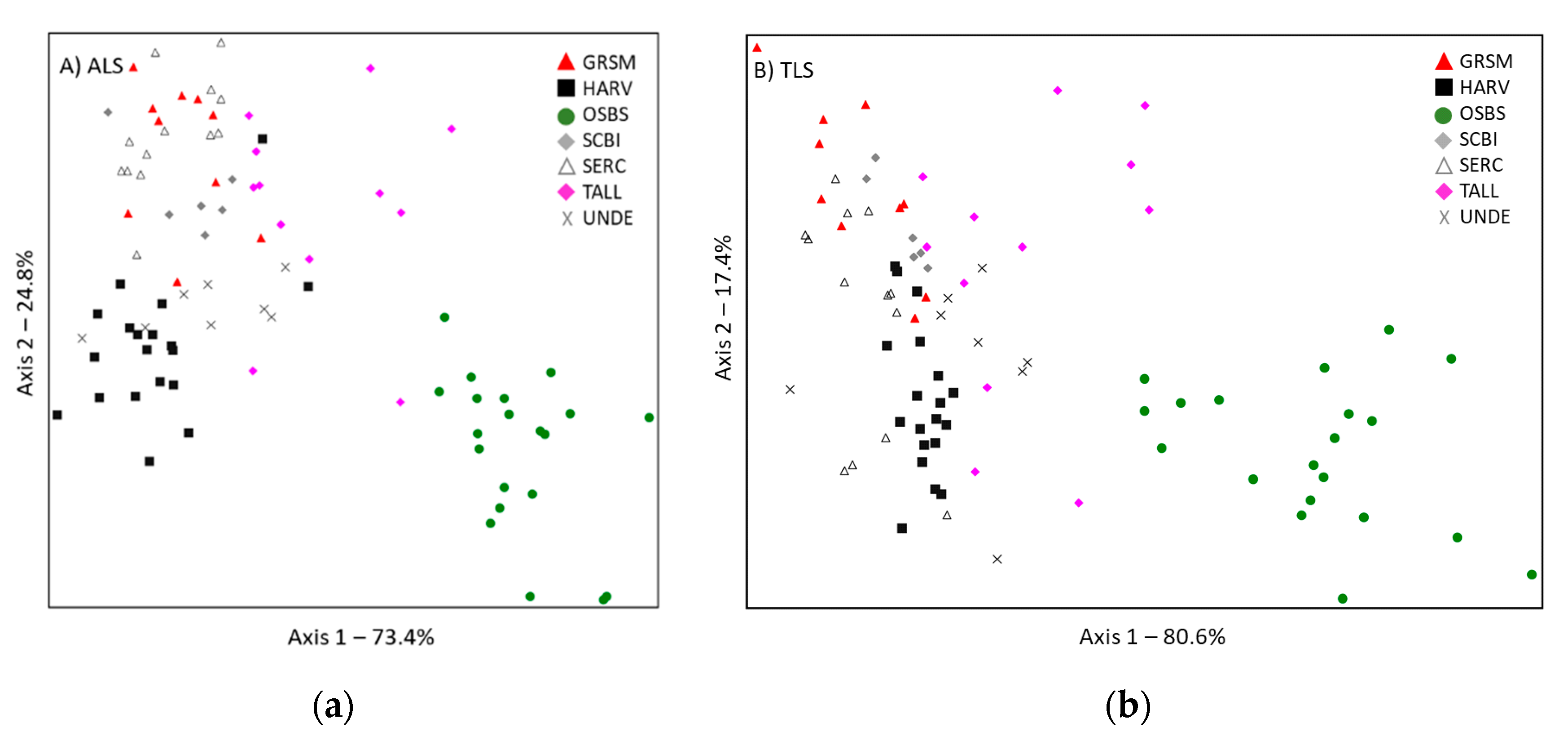
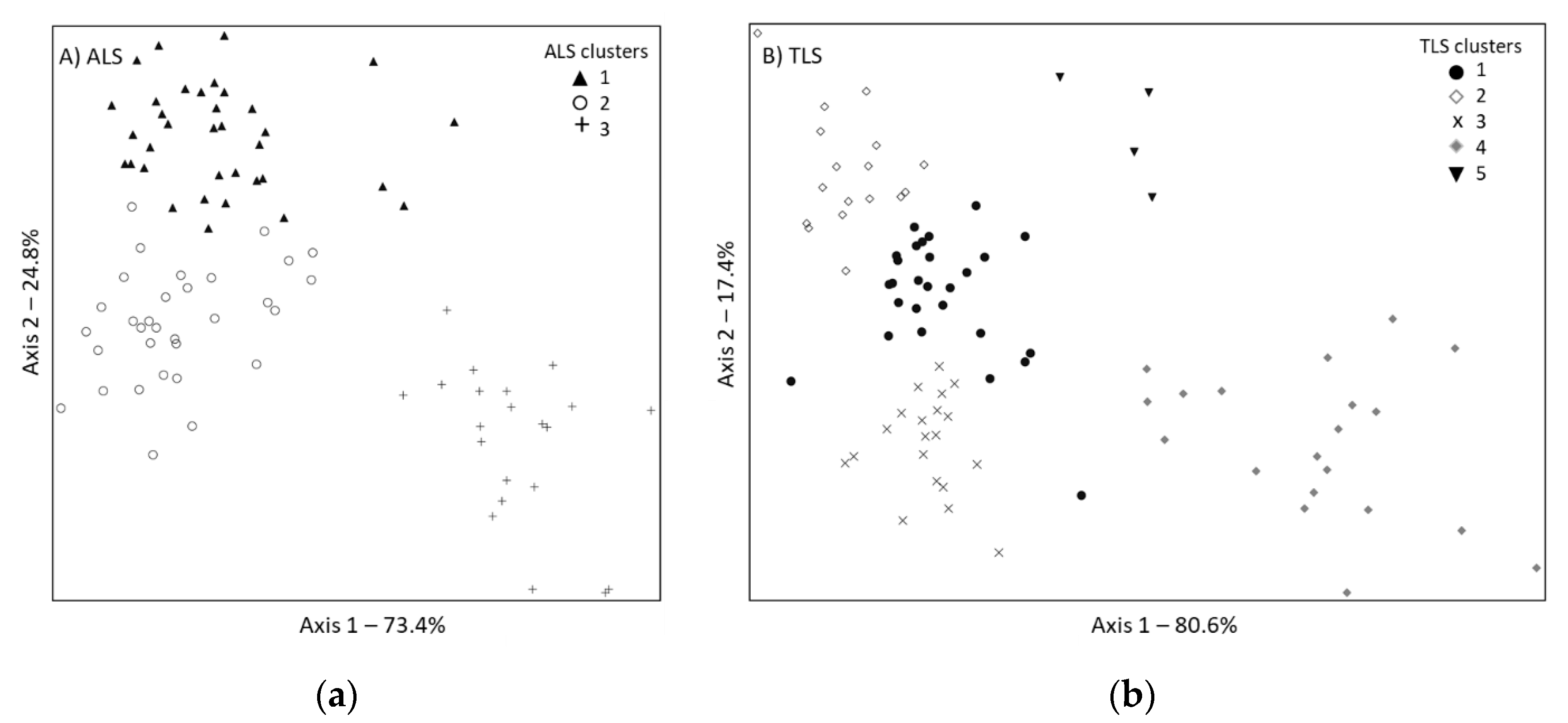
3.2. Multivariate Comparison of ALS and TLS Classifications

There was strong agreement in the general multivariate classification of plots from different forest sites by ALS and TLS metrics of structural diversity (Figure 4), demonstrating the ability of both systems to resolve forest type differences at the macroscale. NMS ordination of structural diversity derived from ALS data had a two-dimensional solution with mean stress of 7.811, which was significant relative to randomized data (p = 0.004) and explained a 98.2% of the variation in the original data matrix (Figure 4a). The first axis explained 73.4% of the variation and was driven most strongly by the vegetation area index (VAI) and maximum canopy height. The second axis explained an additional 24.8% of the variation and was most strongly driven by vertical variation in canopy height. There was a relatively strong separation between sites in the ALS-based ordination space (Figure 4a), and MRPP analysis indicated significant differences among sites in structural diversity (A = 0.50, p < 0.001). Classification of the TLS structural diversity metrics was also explained in two dimensions of multivariate structural space (Figure 4b). The NMS ordination based on TLS structural diversity metrics had a two-dimensional solution that was significant relative to randomized data (p = 0.004; mean stress = 8.665) and explained a 97.9% of the variation in the original data matrix. The first axis explained 80.6% of the variation and was driven by vegetation area and openness. The second axis explained an additional 17.4% of the variation and was driven by canopy height and internal heterogeneity. NMS ordination of structural diversity derived from TLS data illustrated differentiation among sites (MRPP analysis A = 0.45, p < 0.001). Both ALS and TLS suites of structural diversity metrics provided a similar two-dimensional characterization of plots from different sites (Figure 4a,b), indicating that both LiDAR systems were able to resolve differences in structural diversity of plots from different forest types at a sub-continental scale.
While there was broad agreement in the clustering of plots from structurally similar forest sites that vary by height and openness from ALS and TLS metrics of structural diversity, the finer resolution of TLS data provided a greater ability to distinguish plots from within sites that have subtle differences in structural diversity (Figure 5, Table 5). Hierarchical agglomerative clustering of TLS and ALS structural metrics produced different numbers of clusters in structural diversity space, indicating that, as expected, TLS and ALS were sensitive to different canopy structural features. ALS structural diversity metrics were clustered into three groups (based on iterative indicator species analysis conducted on grouping levels; minimum average p-value in three cluster solutions: p = 0.0002) (Table 5). These three groups separated plots from sites approximately by geography (latitude) with groups of northern (medium height and high canopy cover), mid-Atlantic/Appalachian (tallest height and high canopy cover), and southern sites (lowest height and open canopy) (Figure 5a). In contrast, TLS structural diversity metrics grouped canopies into five clusters (minimum mean p-value from Indicator species analysis [ISA] – p = 0.001) (Table 5). These clusters split the plots from the following groups of sites: HARV/SERC, GRSM/SERC, UNDE/SCBI, OSBS, and a subset of TALL (Figure 5b). The additional groupings distinguished by the TLS data were related to plots with very tall canopy but low complexity (cluster 5 – TALL site), plots with short canopy but high VAI (cluster 3 – largely at HARV and UNDE), and plots with extreme vertical complexity (cluster 2 – largely GRSM and SERC). A comparison of the groupings of plots into clusters using the two different data sets illustrated both substantial agreement in some regards and separation in others (Table 5). The two classification systems agreed to place the OSBS plots into a distinct cluster group, while the other two ALS clusters aggregated plots largely from 2 or 3 of the TLS clusters, respectively. The ability of the TLS to split plots from different sites into clusters with plots from other sites illustrated that TLS permitted the characterization of within-site variability of structural diversity versus the purely among-site variation that was represented in the ALS ordination and clustering (Figure 5a,b).

4. Discussion

Despite terrestrial and aerial LiDAR systems having trade-offs in their resolution and spatial extent for the characterization of structural diversity, the results of our study showed broad agreement between ALS and TLS in the potential to quantify canopy structural diversity across a variety of forest types at a sub-continental scale. We showed robust concurrence among equivalent measures of canopy height, cover and openness, vegetation area, and internal heterogeneity. We also showed that ALS delineated the multivariate canopy structural types among forest sites at a sub-continental scale. Our results demonstrated that low resolution, large footprint ALS systems might be a useful tool for classifying forests by structural diversity at landscape to sub-continental scales. However, TLS-derived metrics may be required to resolve fine-scale structural variation within forest types, such as that related to disturbance history, management, or successional development [34,45]. Previous studies have focused on comparisons of ALS and TLS at a single site or forest type in a localized region, but consistent with our results, these have found that ALS and TLS are comparable in their capacity to delineate features, such as canopy height, cover, and vertical stratification [23,34,35,36]. TLS systems are a well-established method to provide high resolution, functionally meaningful measurements of structural diversity in forest ecosystems at the stand-scale [2,19,20,22,35,46], but these results demonstrate that ALS could potentially be used to scale the characterization of canopy structural diversity to much broader spatial extents.
The effects of occlusion that plague both bottom-up TLS and top-down ALS methods did not prevent robust agreement for 8 of the 10 equivalent metrics tested here but did result in a low agreement for two metrics of external heterogeneity. The top-down view of ALS versus the bottom-up viewing angle of TLS resulted in a difference in laser beam attenuation that might mean these systems saw non-overlapping portions of the canopy volume (Figure 1). Specifically, ALS typically exhibits decreased capacity to resolve sub-canopy vegetation relative to TLS due to increased attenuation. However, ALS has been shown to be able to resolve layer differences in multi-level forest canopies in combination with robust predictive models [47]. Meanwhile, TLS exhibits a decreased ability to clearly characterize upper canopy elements relative to ALS, also due to increased attenuation [36]. The partial occlusion of the canopy surface in TLS data was apparent in our study, as univariate analyses illustrated only partial agreement among measures of external canopy heterogeneity that estimated structural diversity at the outer canopy surface. A similar issue was observed by Hilker et al. [23], who found that while TLS accurately measured canopy height from the top 10% of points, it underestimated total canopy height by approximately a meter. This suggests a need for caution in relying on the portable canopy TLS [22] for measuring outer canopy features (e.g., external heterogeneity), whereas ALS seems better suited for this category of structural diversity metric. Nevertheless, the broad agreement we observed between ALS and TLS methods for quantifying most categories of structural diversity metrics supported the use of ALS to scale up functionally relevant measurements of canopy structure and further suggested that structural metrics derived from ALS could serve as a reasonable proxy for TLS-derived metrics (e.g., [47]). Recent advances in new LiDAR technologies (e.g., full-waveform LiDAR, Geiger mode, or United States Geological Survey level-1 aggregates of a nominal pulse density 8 pts/m) and new computational algorithms are beginning to help reduce occlusion issues that hinder ALS, which may result in an even stronger agreement between ALS and TLS for measuring structural diversity. ALS is useful for measuring structural diversity metrics; however, future research that incorporates these technological and computational advances could further improve the measurement of forest structural diversity.
The relatively low resolution of ALS is sufficient to distinguish between different forest sites based on multivariate structural diversity, but TLS is better suited to resolving within site variation. In our study, there was a similar placement of plots from different forest types in multivariate space based on ALS and TLS structural diversity metrics. These seven forest sites spanned an ecological gradient across six of NEON’s ecoclimatic domains, which might enhance our ability to identify unique clusters of structural diversity types. However, there were both similarities and differences in the hierarchical agglomerative clustering by TLS (five clusters) and ALS (three clusters). For example, OSBS, a pine savannah characterized by open canopies and short trees, was always placed in its own cluster by both LiDAR platforms. This illustrated the ability to clearly delineate general structural types among different forests for ALS or TLS. Forest sites with denser canopies, dominated by deciduous species (which tend to have broader, rounded crowns), did not cluster similarly and were split among four TLS clusters and two from ALS. This indicated that studies seeking to investigate fine-scale differences in structural diversity within a forest type or single site should rely on TLS to accurately characterize the sub-canopy structure. There are ecological and management circumstances for which it is desirable to resolve fine-scale structural variation and its role in forest ecosystem function; for example, to understand differences in a local disturbance on the same forest type [34] or to assess the effects of forest management actions [48]. However, previous studies have demonstrated that at larger scales, greater variation in structural diversity occurs across forest types and sites rather than within sites [2,18,49]. For example, canopy structural types defined using multi-dimensional metrics of three-dimensional forest structure are useful for predicting forest productivity [7]. The applicability of ALS to delineate structural diversity types in forest transitional zones has yet to be rigorously tested, but we hypothesized that the within-type structural variability might be high, while the among-type variability would be low for different forest types. Transitional forest types on a landscape-level would likely create additional clusters to those that we found in the ALS multivariate analysis here. We suggest that the derivation of some canopy traits and general canopy structural types across landscapes is feasible with ALS and that ALS could be an appropriate choice for characterizing broad-scale forest variation in forest macrosystem studies (e.g., [50]). We also caution users of ALS to keep the context of structural attributes of forests in mind because resolving structural diversity in the sub-canopy of open canopies will be easier than dense, closed canopies that pose occlusion issues for low-density ALS.

5. Conclusions

The TLS and ALS systems were compared here, with each providing unique benefits for remotely sensing forest structural diversity, and both could be robustly applied across different forest types at a sub-continental scale. The portable canopy LiDAR TLS system we examined was extremely portable and efficient at collecting within-canopy structural diversity data at stand scales—making this TLS system useful in small-scale structural diversity analyses where higher point densities are needed. The ALS system had the capacity to measure structural diversity at broader scales, which was advantageous for investigating spatial and temporal dynamics or testing compatibility to model simulations that use space-borne remote sensing data at larger extents than is feasible to measure with TLS systems. Furthermore, future studies should also compare remotely sensed measures of structural diversity with forest-inventory-based structural diversity metrics (e.g., [9]) because forest managers often make management decisions based predominantly on inventory metrics. Advances in the open-source coding and the accessibility of ALS, from organizations, such as NEON, have a distinct capacity to quantify forest canopy structural diversity at scales that have not been possible until recently. These improvements allow for the incorporation of more comprehensive structural information in ecological models, forest management, and strategic decision making for forest macrosystems. Understanding the limitations and shortcomings of ALS and TLS LiDAR systems, and how we can utilize the complementary strengths of these systems, is a critical step forward for further understanding the complex dynamics that link forest structural diversity with macroscale patterns of ecosystem functioning.

Supplementary Materials

The following are available online at https://www.mdpi.com/2072-4292/12/9/1407/s1, Table S1. Derivation of structural diversity metrics from aerial laser scanning (ALS). Supplementary methods: 1. Spatial stability of ALS metrics estimated from the TLS 2D canopy slice approach, Figure S1: Breakpoint analysis for VAI, mean outer canopy height, and maximum canopy height, Figure S2: Breakpoint analysis for top rugosity, the standard deviation of the standard deviation of height, entropy, VCI, the standard deviation of height, and rumple, Figure S3: Breakpoint analysis for cover fraction, deep gaps, deep gap fraction, and gap fraction profile.

Author Contributions

S.F. and B.S.H. conceived the idea. F.W.W. and E.A.L. wrote the initial draft. E.A.L., F.W.W., J.W.A., and S.F. conducted analyses. All authors have read and agreed to the published version of the manuscript.

Funding

Funding for this work was supported by NSF award #1638702 to S. Fei and B. Hardiman, NSF award #1924942 to S. Fei, B. Hardiman, and E. LaRue, NSF award # 1926538 to B. Hardiman, and USDA Forest Service award #19-JV-11242305-102 to S. Fei.

Acknowledgments

We thank three anonymous reviewers for improving the manuscript.

Conflicts of Interest

The authors declare no conflict of interest.

References

  1. LaRue, E.A.; Hardiman, B.S.; Elliott, J.M.; Fei, S. Structural diversity as a predictor of ecosystem function. Environ. Res. Lett. 2019, 14, 114011. [Google Scholar] [CrossRef]
  2. Atkins, J.W.; Bohrer, G.; Fahey, R.T.; Hardiman, B.S.; Morin, T.H.; Stovall, A.E.L.; Gough, C.M. Quantifying vegetation and canopy structural complexity from TLS data using the forestr r package. Methods Ecol. Evol. 2018, 9, 2057–2066. [Google Scholar] [CrossRef]
  3. Niinemets, U. Photosynthesis and resource distribution through plant canopies. Plant Cell Environ. 2007, 30, 1052–1071. [Google Scholar] [CrossRef] [PubMed]
  4. Matheny, A.M.; Bohrer, G.; Garrity, S.R.; Morin, T.H.; Howard, C.J.; Vogel, C.S. Observations of stem water storage in trees of opposing hydraulic strategies. Ecosphere 2015, 6, 1–13. [Google Scholar] [CrossRef] [Green Version]
  5. Hardiman, B.S.; Gough, C.M.; Halperin, A.; Hofmeister, K.L.; Nave, L.E.; Bohrer, G.; Curtis, P.S. Maintaining high rates of carbon storage in old forests: A mechanism linking canopy structure to forest function. For. Ecol. Manag. 2013, 298, 111–119. [Google Scholar] [CrossRef]
  6. Fotis, A.T.; Morin, T.H.; Fahey, R.T.; Hardiman, B.S.; Bohrer, G.; Curtis, P.S. Forest structure in space and time: Biotic and abiotic determinants of canopy complexity and their effects on net primary productivity. Agric. For. Meteorol. 2018, 250, 181–191. [Google Scholar] [CrossRef]
  7. Fahey, R.T.; Atkins, J.W.; Gough, C.M.; Hardiman, B.S.; Nave, L.E.; Tallant, J.M.; Nadehoffer, K.J.; Vogel, C.; Scheuermann, C.M.; Stuart-Haëntjens, E.; et al. Defining a spectrum of integrative trait-based vegetation canopy structural types. Ecol. Lett. 2019, 22, 2049–2059. [Google Scholar] [CrossRef]
  8. Ehbrecht, M.; Schall, P.; Ammer, C.; Seidel, D. Quantifying stand structural complexity and its relationship with forest management, tree species diversity and microclimate. Agric. For. Meteorol. 2017, 242, 1–9. [Google Scholar] [CrossRef]
  9. McElhinny, C.; Gibbons, P.; Brack, C.; Bauhus, J. Forest and woodland stand structural complexity: Its definition and measurement. For. Ecol. Manag. 2005, 218, 1–24. [Google Scholar] [CrossRef]
  10. Atkins, J.W.; Bohrer, G.; Fahey, R.T.; Hardiman, B.S.; Gough, C.M.; Morin, T.H.; Stovall, A.; Zimmerman, N. Forestr: Ecosystem and Canopy Structural Complexity Metrics from LiDAR; R Package Version 1.0.1; 2018; Available online: https://cran.r-project.org/web/packages/forestr/ (accessed on 1 January 2018).
  11. Wilkes, P.; Disney, M.; Vicari, M.B.; Calders, K.; Burt, A. Estimating urban above ground biomass with multi-scale LiDAR. Carbon Balanc. Manag. 2018, 13, 10. [Google Scholar] [CrossRef]
  12. Fisher, R.A.; Koven, C.D.; Anderegg, W.R.L.; Christoffersen, B.O.; Dietze, M.C.; Farrior, C.E.; Moorcroft, P.R. Vegetation demographics in Earth System Models: A review of progress and priorities. Glob. Chang. Biol. 2018, 24, 35–54. [Google Scholar] [CrossRef] [PubMed] [Green Version]
  13. Shiklomanov, A.N.; Bradley, B.A.; Dahlin, K.M.; M Fox, A.; Gough, C.M.; Hoffman, F.M.; M Middleton, E.; Serbin, S.P.; Smallman, L.; Smith, W.K. Enhancing global change experiments through integration of remote-sensing techniques. Front. Ecol. Environ. 2019, 17, 215–224. [Google Scholar] [CrossRef] [Green Version]
  14. Lefsky, M.A.; Cohen, W.B.; Harding, D.J.; Parker, G.G.; Acker, S.A.; Gower, S.T. LiDAR remote sensing of above-ground biomass in three biomes. Glob. Ecol. Biogeogr. 2002, 11, 393–399. [Google Scholar] [CrossRef] [Green Version]
  15. Lim, K.; Treitz, P.; Wulder, M.; St-Onge, B.; Flood, M. LiDAR remote sensing of forest structure. Prog. Phys. Geogr. Earth Environ. 2003, 1, 88–106. [Google Scholar] [CrossRef] [Green Version]
  16. Nguyen, H.T.; Hutyra, L.R.; Hardiman, B.S.; Raciti, S.M. Characterizing forest structure variations across an intact tropical peat dome using field samplings and airborne LiDAR. Ecol. Appl. 2016, 26, 587–601. [Google Scholar] [CrossRef] [PubMed]
  17. Disney, M.I.; Boni Vicari, M.; Burt, A.; Calders, K.; Lewis, L.; Raumonen, P.; Wilkes, P. Weighing trees with lasers: Advances, challenges and opportunities. Interface Focus 2018, 8, 20170048. [Google Scholar] [CrossRef] [Green Version]
  18. LaRue, E.A.; Atkins, J.W.; Dahlin, K.; Fahey, R.; Fei, S.; Gough, C.; Hardirnan, B.S. Linking Landsat to terrestrial LiDAR: Vegetation metrics of forest greenness are correlated with canopy structural complexity. Int. J. Appl. Earth Obs. Geoinf. 2018, 73, 420–427. [Google Scholar] [CrossRef]
  19. Paynter, I.; Genest, D.; Saenz, E.; Peri, F.; Boucher, P.; Li, Z.; Strahler, A.; Schaaf, C. Classifying ecosystems with metaproperties from terrestrial laser scanner data. Methods Ecol. Evol. 2018, 9, 210–222. [Google Scholar] [CrossRef] [Green Version]
  20. Newnham, G.J.; Armston, J.D.; Calders, K.; Disney, M.I.; Lovell, J.L.; Schaaf, C.B.; Strahler, A.H.; Danson, F.M. Terrestrial Laser Scanning for Plot-Scale Forest Measurement. Curr. For. Rep. 2015, 1, 239–251. [Google Scholar] [CrossRef] [Green Version]
  21. Lefsky, M.A.; Cohen, W.B.; Parker, G.G.; Harding, D.J. LiDAR remote sensing for ecosystem studies. Bioscience 2002, 52, 19–30. [Google Scholar] [CrossRef]
  22. Parker, G.G.; Harding, D.J.; Berger, M.L. A portable LiDAR system for rapid determination of forest canopy structure. J. Appl. Ecol. 2004, 41, 755–767. [Google Scholar] [CrossRef]
  23. Hilker, T.; Coops, N.C.; Newnham, G.J.; van Leeuwen, M.; Wulder, M.A.; Stewart, J.; Culvenor, D.S. Comparison of terrestrial and airborne LiDAR in describing stand structure of a thinned lodgepole pine forest. J. For. 2012, 110, 97–104. [Google Scholar] [CrossRef]
  24. Wing, B.M.; Ritchie, M.W.; Boston, K.; Cohen, W.B.; Gitelman, A.; Olsen, M.J. Prediction of understory vegetation cover with airborne lidar in an interior ponderosa pine forest. Remote Sens. Environ. 2012, 124, 730–741. [Google Scholar] [CrossRef]
  25. Ferraz, A.; Bretar, F.; Jacquemoud, S.; Gonçalves, G.; Pereira, L.; Tomé, M.; Soares, P. 3-D mapping of a multi-layered Mediterranean forest using ALS data. Remote Sens. Environ. 2012, 121, 210–223. [Google Scholar] [CrossRef]
  26. Campbell, M.J.; Dennison, P.E.; Hudak, A.T.; Parham, L.M.; Butler, B.W. Quantifying understory vegetation density using small-footprint airborne lidar. Remote Sens. Environ. 2018, 215, 330–342. [Google Scholar] [CrossRef]
  27. Venier, L.A.; Swystun, T.; Mazerolle, M.J.; Kreutzweiser, D.P.; Wainio-Keizer, K.L.; McIlwrick, K.A.; Woods, M.E.; Wang, X. Modelling vegetation understory cover using LiDAR metrics. PLoS ONE 2019, 14, e0220096. [Google Scholar] [CrossRef] [Green Version]
  28. Hamraz, H.; Contreras, M.A.; Zhang, J. Forest understory trees can be segmented accurately within sufficiently dense airborne laser scanning point clouds. Sci. Rep. 2017, 7, 1–9. [Google Scholar] [CrossRef] [Green Version]
  29. Hamraz, H.; Contreras, M.A.; Zhang, J. Vertical stratification of forest canopy for segmentation of understory trees within small-footprint airborne LiDAR point clouds. ISPRS J. Photogramm. Remote Sens. 2017, 130, 385–392. [Google Scholar] [CrossRef] [Green Version]
  30. Kankare, V.; Vauhkonen, J.; Tanhuanpää, T.; Holopainen, M.; Vastaranta, M.; Joensuu, M.; Krooks, A.; Hyyppä, J.; Hyyppä, H.; Alho, P.; et al. Accuracy in estimation of timber assortments and stem distribution—A comparison of airborne and terrestrial laser scanning techniques. ISPRS J. Photogramm. Remote Sens. 2014, 97, 89–97. [Google Scholar] [CrossRef]
  31. Trochta, J.; Kruček, M.; Vrška, T.; Kraâl, K. 3D Forest: An application for descriptions of three-dimensional forest structures using terrestrial LiDAR. PLoS ONE 2017, 12, e0176871. [Google Scholar] [CrossRef] [Green Version]
  32. Wang, Y.; Lehtomäki, M.; Liang, X.; Pyörälä, J.; Kukko, A.; Jaakkola, A.; Liu, J.; Feng, Z.; Chen, R.; Hyyppä, J. Is field-measured tree height as reliable as believed—A comparison study of tree height estimates from field measurement, airborne laser scanning and terrestrial laser scanning in a boreal forest. ISPRS J. Photogramm. Remote Sens. 2019, 147, 132–145. [Google Scholar] [CrossRef]
  33. Liang, X.; Wang, Y.; Pyörälä, J.; Lehtomäki, M.; Yu, X.; Kaartinen, H.; Kukko, A.; Honkavaara, E.; Issaoui, A.E.I.; Nevalainen, O.; et al. Forest in situ observations using unmanned aerial vehicle as an alternative of terrestrial measurements. For. Ecosyst. 2019, 6, 20. [Google Scholar] [CrossRef] [Green Version]
  34. Listopad, C.M.C.S.; Drake, J.B.; Masters, R.E.; Weishampel, J.F. Portable and airborne small footprint LiDAR: Forest canopy structure estimation of fire managed plots. Remote Sens. 2011, 3, 1284–1307. [Google Scholar] [CrossRef] [Green Version]
  35. Hopkinson, C.; Lovell, J.; Chasmer, L.; Jupp, D.; Kljun, N.; van Gorsel, E. Integrating terrestrial and airborne LiDAR to calibrate a 3D canopy model of effective leaf area index. Remote Sens. Environ. 2013, 136, 301–314. [Google Scholar] [CrossRef]
  36. Hilker, T.; van Leeuwen, M.; Coops, N.C.; Wulder, M.A.; Newnham, G.J.; Jupp, D.L.B.; Culvenor, D.S. Comparing canopy metrics derived from terrestrial and airborne laser scanning in a Douglas-fir dominated forest stand. Trees Struct. Funct. 2010, 24, 819–832. [Google Scholar] [CrossRef]
  37. Braun, L. Deciduous Forests of Eastern North America; Hafner: New York, NY, USA, 1950. [Google Scholar]
  38. Atkins, J.W.; Fahey, R.T.; Hardiman, B.S.; Gough, C.M. Forest Canopy Structural Complexity and Light Absorption Relationships at the Subcontinental Scale. J. Geophys. Res. Biogeosci. 2018, 123, 1387–1405. [Google Scholar] [CrossRef]
  39. Team, R.D.C. R: A Language and Environment for Statistical Computing; R Foundation for Statistical Computing: Vienna, Austria, 2019; ISBN 3-900051-07-0. Available online: http://www.R-project.org (accessed on 30 July 2018).
  40. National Ecological Observatory Network. Data Products: DP1.30003.001; Battelle: Boulder, CO, USA, 2019; Available online: http://data.neonscience.org (accessed on 1 January 2019).
  41. Roussel, J.R.; Auty, D. LidR: Airborne LiDAR Data Manipulation and Visualization for Forestry Applications; R Package Version, Version 1.3.1; 2018; Available online: https://cran.r-project.org/web/packages/lidR (accessed on 30 July 2018).
  42. Silva, C.A.; Crookston, N.L.; Hudak, A.T.; Vierling, L.A.; Klauberg, C.; Cardil, A. rLiDAR: LiDAR Data Processing and Visualization; R Package Version 0.1.1; 2017; Available online: https://cran.r-project.org/web/packages/rLiDAR (accessed on 30 August 2018).
  43. McCune, B.; Mefford, M.J. PC-ORD. Multivariate Analysis of Ecological Data, Version 5.0 for Windows; MjM Software: Gleneden Beach, OR, USA, 2006. [Google Scholar]
  44. Mccune, B.; Grace, J. Analysis of Ecological Communities; MJM Software Design: Gleneden Beach, OR, USA, 2002. [Google Scholar]
  45. Meadows, M.E.; Hill, T.R. Issues in Biogeography: Diversity in theory and practice. S. Afr. Geogr. J. 2012, 6245, 116–124. [Google Scholar] [CrossRef]
  46. Paynter, I.; Saenz, E.; Genest, D.; Peri, F.; Erb, A.; Li, Z.; Wiggin, K.; Muir, J.; Raumonen, P.; Schaaf, E.S.; et al. Observing ecosystems with lightweight, rapid-scanning terrestrial lidar scanners. Remote Sens. Ecol. Conserv. 2016, 2, 174–189. [Google Scholar] [CrossRef]
  47. Mund, J.-P.; Wilke, R.; Körner, M.; Schultz, A. Detecting Multi-layered Forest Stands Using High Density Airborne LiDAR Data. J. Geogr. Inf. Sci. 2015, 1, 178–188. [Google Scholar] [CrossRef]
  48. Donager, J.J.; Sankey, T.T.; Sankey, J.B.; Sanchez Meador, A.J.; Springer, A.E.; Bailey, J.D. Examining forest structure with terrestrial lidar: Suggestions and novel techniques based on comparisons between scanners and forest treatments. Earth Space Sci. 2018, 5, 753–776. [Google Scholar] [CrossRef] [Green Version]
  49. Gough, C.M.; Atkins, J.W.; Fahey, R.T.; Hardiman, B.S. High rates of primary production in structurally complex forests. Ecology 2019, 100, e02864. [Google Scholar] [CrossRef] [PubMed] [Green Version]
  50. Kleindl, W.; Stoy, P.; Binford, M.W.; Desai, A.R.; Dietze, M.C.; Schultz, C.A.; Starr, G.; Staudhammer, C.L.; Wood David, J.A. Toward a Social-Ecological Theory of Forest Macrosystems for Improved Ecosystem Management. Forests 2018, 9, 200. [Google Scholar] [CrossRef] [Green Version]
Figure 1. Comparison of aerial laser scanning (ALS) and terrestrial laser scanning (TLS) point clouds for the Great Smoky Mountains site of the National Ecological Observatory Network at plot 053 (40 × 40 m) from oblique, overhead, and side angles. Vertical profiles of return heights from raw LiDAR returns demonstrate the occlusion experienced by both LiDAR methods as a result of their respective view angles (return density refers to the proportion of total points or relative densities of returns from each platform).
Remotesensing 12 01407 g001
Figure 2. Seven forested sites (see Table 1 for site descriptions) from the National Ecological Observatory Network across the eastern USA measured by aerial laser scanning (ALS) and terrestrial laser scanning (TLS).
Remotesensing 12 01407 g002
Figure 3. Pairwise Spearman correlation coefficients between aerial laser scanning (ALS) (Y-axis) and terrestrial laser scanning (TLS) metrics (X-axis). Boxes show the paired correlation coefficient results, and the colors of the squares indicate the strength of each correlation; an X indicates a relationship was not significant at α < 0.05.
Remotesensing 12 01407 g003
Figure 4. Non-metric multidimensional scaling ordination, illustrating variation in multivariate classification of plots across seven forest sites from structural diversity as measured using (a) aerial laser scanning (ALS) and (b) terrestrial laser scanning (TLS). Site ID abbreviations can be found in Table 1.
Remotesensing 12 01407 g004
Figure 5. Illustration of canopy structural type groupings derived from hierarchical agglomerative clustering overlaid on non-metric multidimensional scaling ordination of structural diversity across seven studied forest sites; (a) illustrates cluster groups derived from aerial laser scanning (ALS) data and (b) cluster groups from terrestrial laser scanning (TLS) data.
Remotesensing 12 01407 g005
Table 1. Seven forested National Ecological Observatory Network sites measured using both terrestrial laser scanning (TLS) and aerial laser scanning (ALS).
Site (ID)Ecoclimatic DomainDominant Forest TypeNPlots
Harvard Forest (HARV)NortheastMixed temperate19
Smithsonian Conservation Biology Institute (SCBI)Mid-AtlanticMixed temperate6
Smithsonian Environmental Research Center (SERC)Mid-AtlanticTemperate deciduous13
Ordway-Swisher Biological Station (OSBS)SoutheastPine Savannah20
University of Notre Dame Environmental Research Center East (UNDE)Great LakesMixed temperate8
Great Smoky Mountain National Park (GRSM)Appalachians and Cumberland PlateauTemperate rainforest10
Talladega National Forest (TALL)Ozarks ComplexPine savannah12
Table 2. Categories of forest structural diversity and metrics from terrestrial laser scanning (TLS) and aerial laser scanning (ALS) platforms. Details on the derivation and R functions used to calculate structural metrics can be found in Atkins et al. [10] for TLS and Supplementary Materials Table S1 for ALS. The abbreviations of metric names are listed in parentheses.
CategoryALS MetricTLS Metric
HeightMean canopy height (H), Mean outer canopy height (MOCH), Maximum canopy height (Hmax) Mean leaf height (Mean H), Mean outer canopy height (MOCH), Maximum canopy height (Max.can.ht), Mean of squared leaf height model (Mode.2), Mode.el (Model.el), Mean height of maximum VAI (Max.el), Root mean square height (meanHRMS), Mean height variability (meanHvar), SD of mean height (Height.2)
Cover and opennessDeep gaps (DG), Deep gap fraction (DGF), Cover fraction (CF), Gap fraction profile (GFP)Deep gaps (DG), Deep gap fraction (DGF), Sky fraction (SF), Cover fraction (CF)
HeterogeneityExternal Top rugosity (TR), Rumple (Rumple)Top rugosity (TR), Rumple (Rumple)
Internal SD of vertical SD of height (StdStd), Entropy (Entropy), Height SD (HSD: rLiDAR), Height SD (StdH: lidR), Vertical complexity index (VCI)Canopy rugosity (Rugosity), Mean of vertical SD (MeanStd), SD of vertical SD (StdStd), Effective number of layers (ENL)
Vegetation areaVegetation area index (VAI)Mean VAI (Mean.VAI), Mean peak VAI (Mean.peak.VAI)
Table 3. LiDAR system specifications for aerial laser scanning (ALS) and terrestrial laser scanning (TLS) platforms.
System SpecificationsOptech ALTM Gemini (ALS)Riegl LD90-3100VHS-FLP (TLS)
Returns per PulseFourFive
Wavelength1064 nm900 nm
Measurement Range150–4000 m60 m (ρ ≥ 0.1)–200 m (ρ ≥ 0.8)
Range Accuracy (typical)± 5–30 cm±2.5 cm
Bean Divergence Angle0.25 mrad × 0.8 mrad3 mrad × 5 mrad
Measurement Rate (per second)0–70 (programmable)2000
Average Point Density1–4 points per m2500–2000 points per linear meter
Laser Product ClassificationClass IV (US FDA 21 CFR)IEC 60825–1:2007 (Eye-safe)
Table 4. Spearman correlations between equivalently estimated structural diversity metrics with terrestrial laser scanning (TLS) and aerial laser scanning (ALS).
CategoryALSTLSr
HeightMOCHMOCH0.80 *
HH0.72 *
HmaxMax.can.ht0.92 *
Cover and opennessDGFDGF0.66 *
CFCF0.74 *
External heterogeneityRumpleRumple0.09
TRTR0.44 *
Internal heterogeneityStdHMeanStd0.61 *
StdStdRugosity0.74 *
Vegetation areaVAIVAI0.87 *
* values were significant at α < 0.05
Table 5. Comparison of plot assignment to groupings derived from hierarchical agglomerative clustering of aerial laser scanning (ALS) and terrestrial laser scanning (TLS), illustrating structural diversity variation in multivariate space between LiDAR platforms. Cluster name indicates which plot was assigned to a given TLS or ALS cluster. Numbers indicate how many plots were assigned to each cluster.
ClusterTLS1TLS2TLS3TLS4TLS5Total
ALS1121540435
ALS2142160032
ALS310020021
Total27172020488

