Article

Assessing Soil Cover Levels during the Non-Growing Season Using Multitemporal Satellite Imagery and Spectral Unmixing Techniques

1
Center for Remote Sensing Applications (CRSA), Mohammed VI Polytechnic University (UM6P), Ben Guerir 43150, Morocco
2
Guelph Science and Technology Branch, Agriculture and Agri-Food Canada (AAFC), Guelph, ON N1G 4S9, Canada
3
Department of Geography, Environment & Geomatics, University of Guelph, Guelph, ON N1G 2W1, Canada
4
Ottawa Research and Development Centre, AAFC, Ottawa, ON K1A 0C6, Canada
5
Geomatics, AAFC, Regina, SK S4P 0M3, Canada
*
Author to whom correspondence should be addressed.
Remote Sens. 2020, 12(9), 1397; https://doi.org/10.3390/rs12091397
Submission received: 26 February 2020 / Revised: 16 April 2020 / Accepted: 25 April 2020 / Published: 28 April 2020
(This article belongs to the Special Issue Remote Sensing of Crop Residue and Non-photosynthetic Vegetation)

Abstract

:
Growing cover or winter crops and retaining crop residue on agricultural lands are considered beneficial management practices to address soil health and water quality. Remote sensing is a valuable tool to assess and map crop residue cover and cover crops. The objective of this study is to evaluate the performance of linear spectral unmixing for estimating soil cover in the non-growing season (November–May) over the Canadian Lake Erie Basin using seasonal multitemporal satellite imagery. Soil cover ground measurements and multispectral Landsat-8 imagery were acquired for two areas throughout the 2015–2016 non-growing season. Vertical soil cover photos were collected from up to 40 residue and 30 cover crop fields for each area (e.g., Elgin and Essex sites) when harvest, cloud, and snow conditions permitted. Images and data were reviewed and compiled to represent a complete coverage of the basin for three time periods (post-harvest, pre-planting, and post-planting). The correlations between field measured and satellite imagery estimated soil covers (e.g., residue and green) were evaluated by coefficient of determination (R2) and root mean square error (RMSE). Overall, spectral unmixing of satellite imagery is well suited for estimating soil cover in the non-growing season. Spectral unmixing using three-endmembers (i.e., corn residue-soil-green cover; soybean residue-soil-green cover) showed higher correlations with field measured soil cover than spectral unmixing using two- or four-endmembers. For the nine non-growing season images analyzed, the residue and green cover fractions derived from linear spectral unmixing using corn residue-soil-green cover endmembers were highly correlated with the field-measured data (mean R2 of 0.70 and 0.86, respectively). The results of this study support the use of remote sensing and spectral unmixing techniques for monitoring performance metrics for government initiatives, such as the Canada-Ontario Lake Erie Action Plan, and as input for sustainability indicators that both require knowledge about non-growing season land management over a large area.

Graphical Abstract

1. Introduction

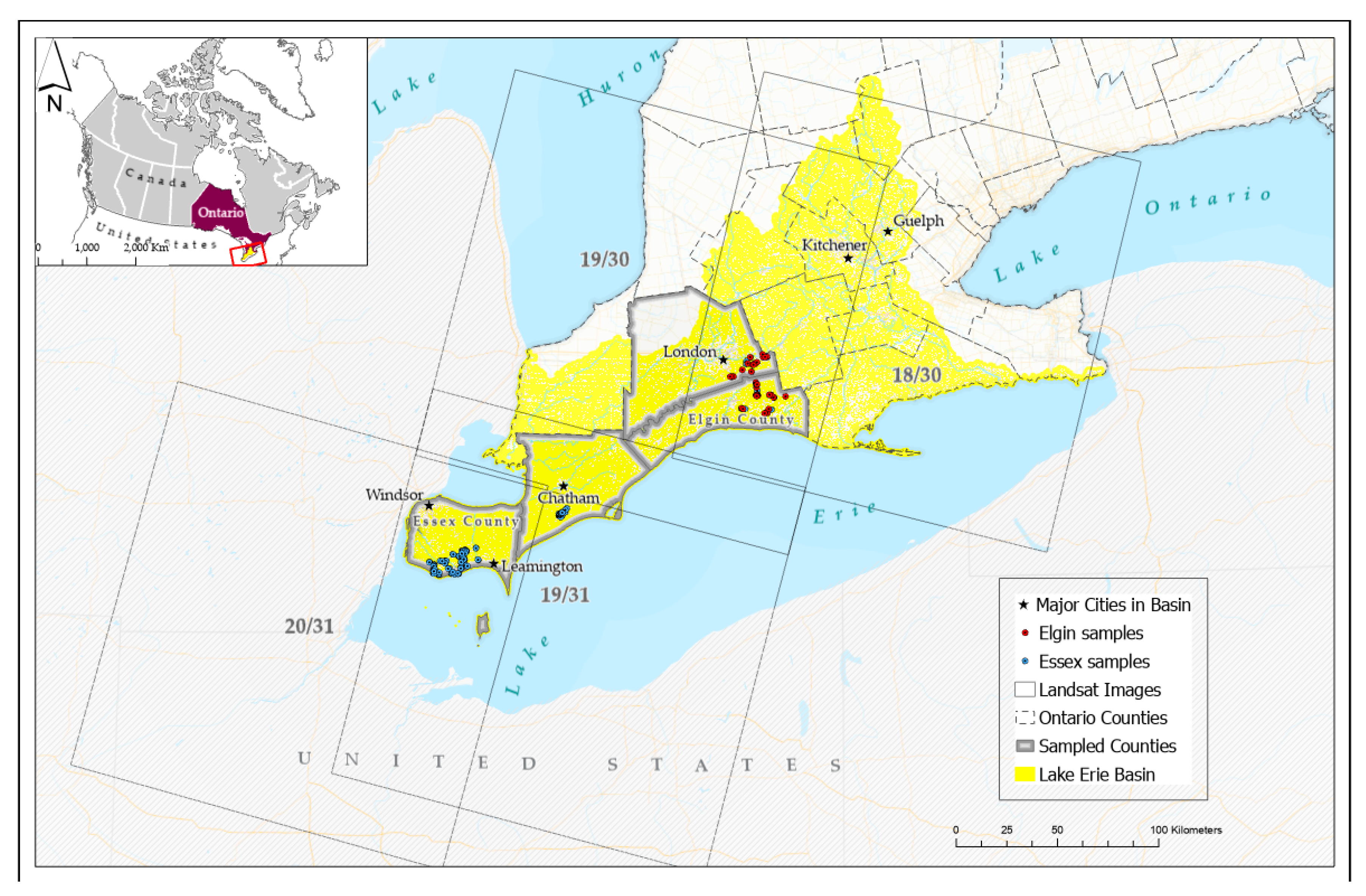
Information about soil cover at a regional scale is important to support modeling and monitoring of agricultural activities, as well as policy and program implementation. There is particular interest in the management of agricultural land in the Lake Erie basin during the non-growing season as this is when most of the non-point source nutrient run-off and loadings to the lake occur. Both crop residues (dead or non-photosynthetic vegetation) and cover/winter crops (living) are considered beneficial for facilitating infiltration and reducing soil erosion and nutrient loss [1,2,3]. Several organizations (e.g., Ontario Ministry of Agriculture, Food and Rural Affairs (OMAFRA), Agriculture and Agri-Food Canada (AAFC), and United States Department of Agriculture (USDA)) are promoting cover crops and retaining crop residue as beneficial management practices (BMPs) to address soil health and water quality and wish to track adoption of these practices [4,5,6]. There is also the question of whether fall tillage/bare soil area may be increasing in the Canadian portion of the basin after years of increases in reduced tillage. Census reporting of no-tillage land preparation for seeding increased from 1991 until 2011, but in 2016 conventional tillage, which incorporates most of the crop residue into the soil, did show an increase [7]. Therefore, improved datasets are needed for agricultural land in the Lake Erie region, that account for the dynamic land cover that changes from year-to-year as a result of adopted crop and tillage rotations. At the Lake Erie Basin scale, these changes in rotations and tillage practices (e.g., no-till or reduced tillage) can collectively have an effect on Great Lakes water quality [8,9,10]).
Crop residue cover is currently measured in the field using one or more conventional methods such as line-transect, meter stick, photographic comparison, hand-held app, or photographic-grid [11,12,13,14]. However, most of these methods are time consuming, labor intensive, and cannot provide continuous data over large areas, as percent residue cover is estimated over spatially and temporally disconnected fields. In the United States, the Conservation Technology Information Center (CTIC) has been instrumental in tracking changes in land management through the Crop Residue Management (CRM) survey which involved county level road-side surveys from 1998–2004 and again in 2006 and 2008 [15]. The CTIC, with Applied Geosolutions and The Nature Conservancy, have now implemented the Operational Tillage Information System (OpTIS) [16,17], a remote sensing-based survey of both tillage and cover crop acres for 645 counties in and around the U.S. Corn Belt Land Resources Region-M, including some in the Lake Erie Basin. To our knowledge, there are no current non-growing season soil cover data or maps (e.g., bare soil, residue, or living crop) for the Canadian Lake Erie Basin. Therefore, it is important to develop methodologies for on-going monitoring of soil cover (cover/winter crops and crop residue) at large scales to meet the needs of land management decision makers.
Many studies have found medium-resolution remote sensing imagery (e.g., Landsat products) to be appropriate for residue and cover crop mapping over large areas [18,19,20,21,22,23,24,25,26,27] given its high overall data quality (e.g., temporal, spatial, and radiometric resolutions). Most of these studies used spectral indices (e.g., the minimum normalized difference tillage index (NDTI) and the Normalized Difference Vegetated Index (NDVI)) to map crop residue cover [28]. Pacheco and McNairn [29] used linear spectral unmixing analysis with multispectral images (e.g., Landsat-5 TM and SPOT-4 and -5) to estimate the fractional abundance of a specific residue type (e.g., corn percentage (%) vs. soybean %) within a single pixel. The authors [
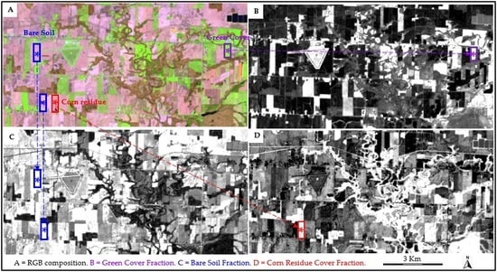
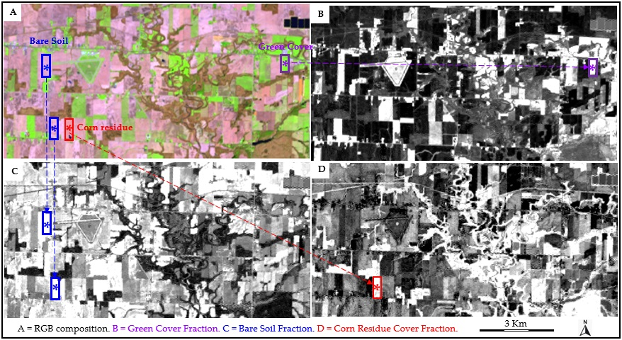
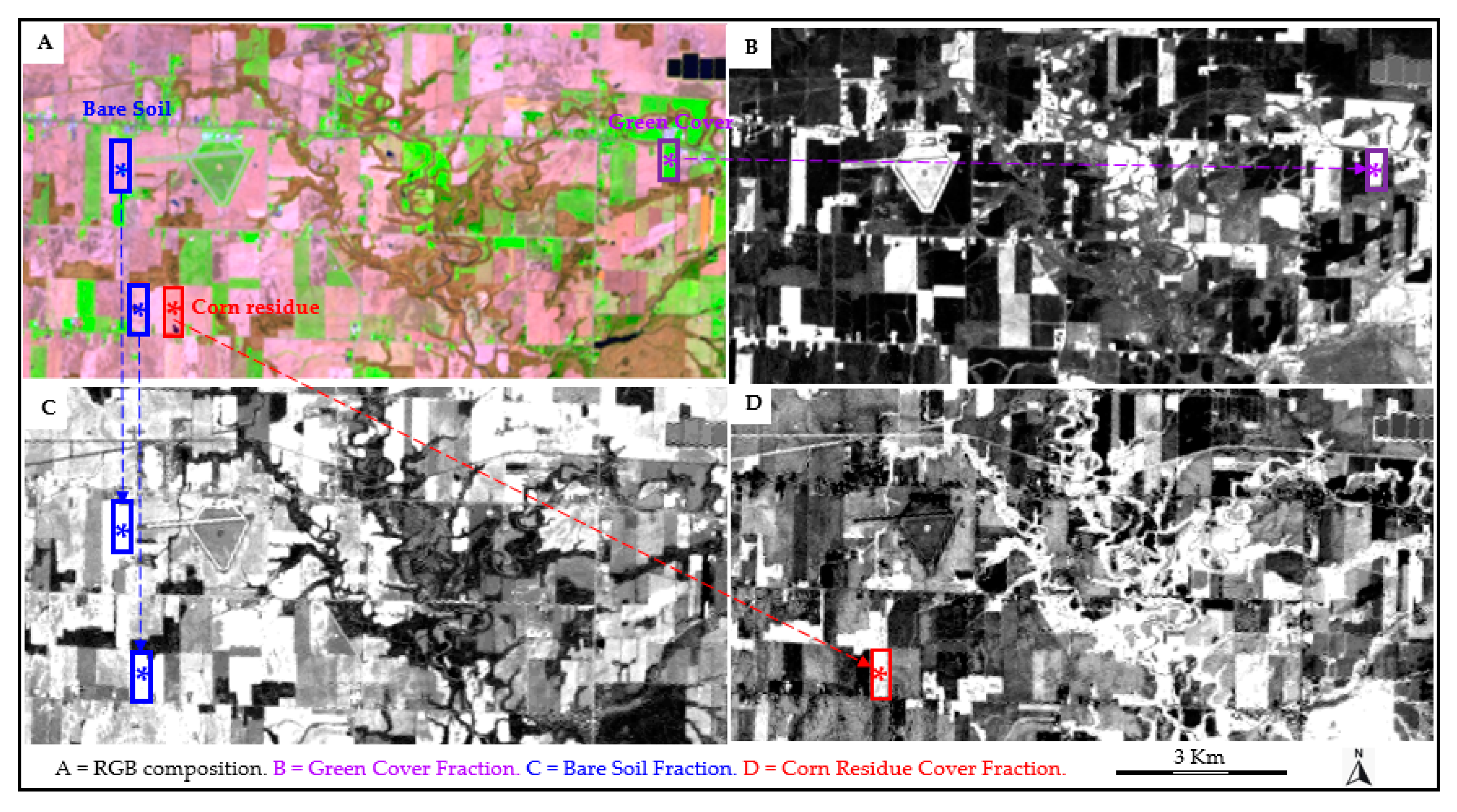
29], thus, demonstrated that the linear spectral unmixing analysis technique is an alternative approach to estimate percent crop residue cover. Unlike spectral indices, spectral unmixing analysis uses the information from all available spectral bands to establish the contribution of soil covers (e.g., crop residue(s), bare soil, green vegetative cover) to total reflectance and generates fraction maps as outputs, which provide the proportion (0 to 1) of each soil cover present in each pixel [29].
In some studies, where only one type of soil cover is studied, pixels or fields have been screened in or out of the study based on a threshold of green cover [30] to improve results. Spectral unmixing which includes both residue and green cover endmembers may be one way to overcome these interference issues and determine both pieces of soil cover information simultaneously [
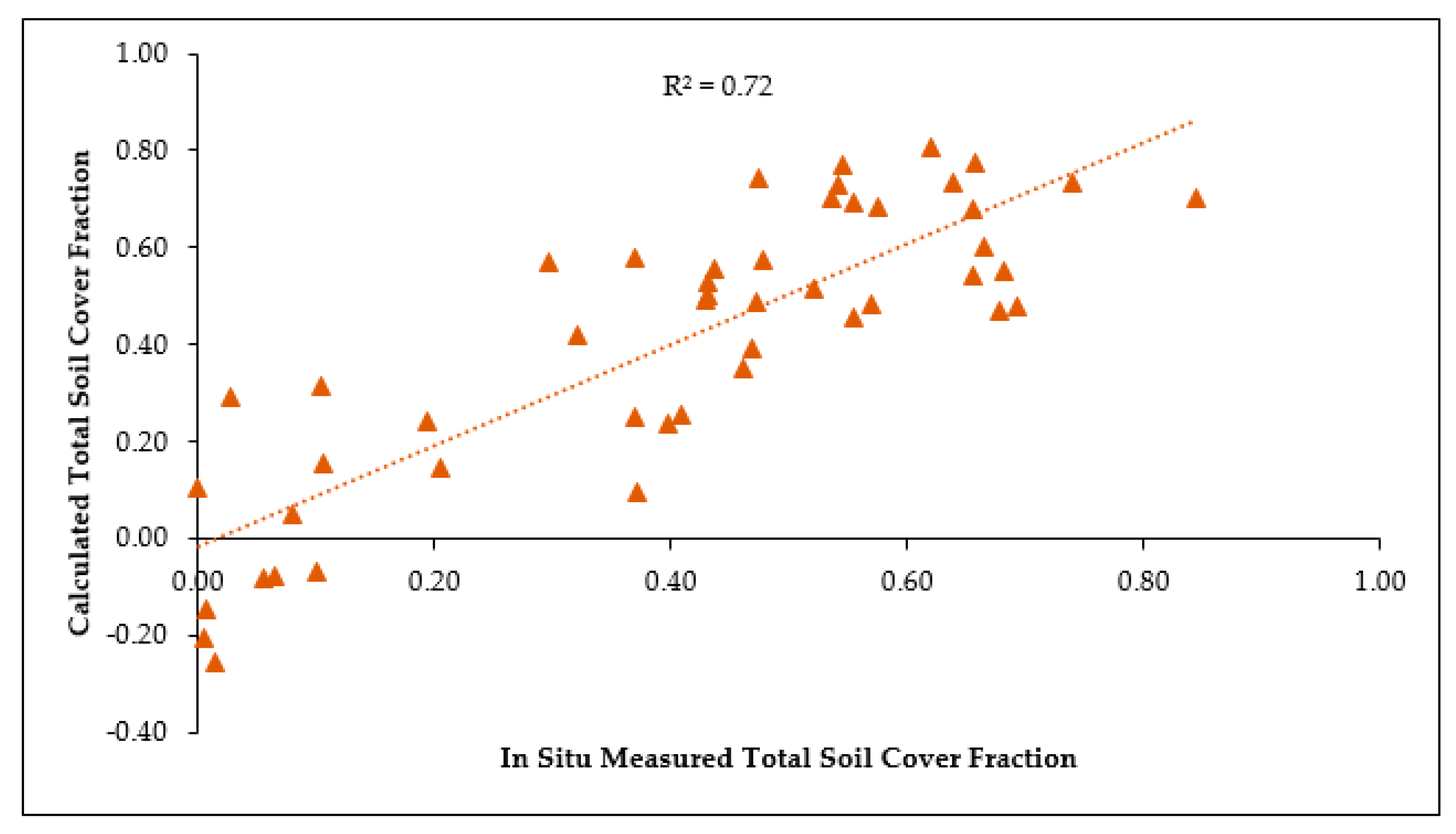
31,32,33], and thereby determine a total soil cover (i.e., total cover = residue + green fraction). In addition, most of the previous medium-resolution remote sensing imagery approaches aimed to map crop residue cover using a single imagery-date; a few studies have used multitemporal remote sensing datasets to monitor crop residue cover changes through time [28,34,35,36,37]. Other studies used multitemporal remote sensing datasets and then selected the minimum NDTI from over the time period [28,36].
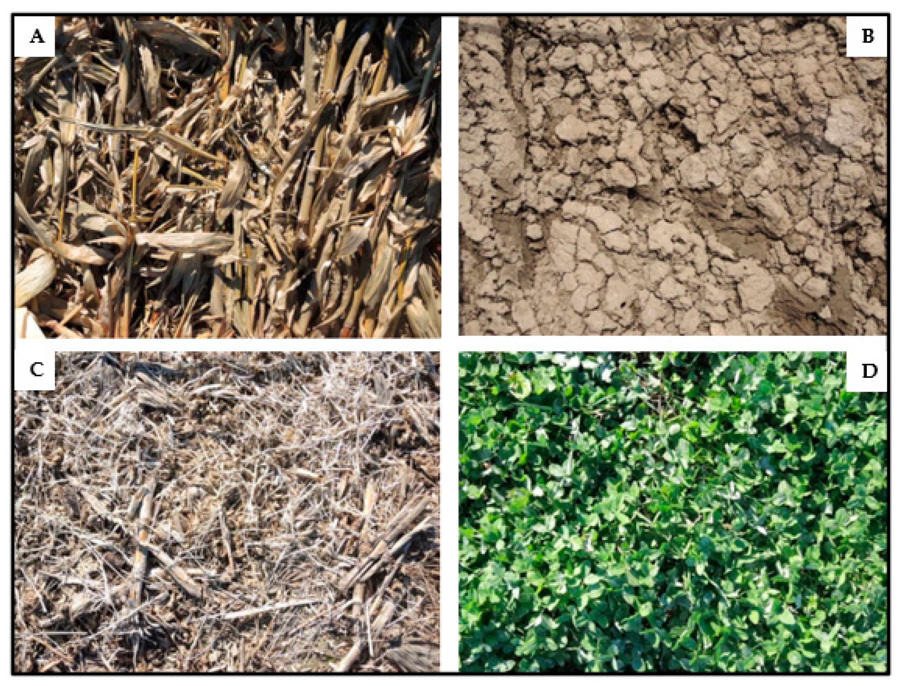
The main objective of this study was to test and evaluate the performance of the linear spectral unmixing analysis technique for estimating soil cover (e.g., bare soil, crop residue, or living crop) using seasonal multitemporal Landsat-8 imagery and to validate against ground measurements over the Canadian Lake Erie Basin. We hypothesize that linear spectral unmixing can be an appropriate technique to map residue and green cover simultaneously, over large geographic regions. More specifically, this study aimed to (i) quantify soil cover fractions for the 2015–2016 non-growing season; (ii) compare the performance of the different possible unmixing endmember combinations; (iii) compare the performance of the best unmixing endmember combination to spectral indices results in relation to ground data; and (iv) evaluate the overall accuracy of residue, green and total cover estimates and classes using the unmixing results.

2. Materials and Methods

2.1. Study Area

This study was conducted in two areas (referred to as Elgin and Essex Counties hereafter; Figure 1), located in the Lake Erie Basin of southwestern Ontario, Canada (Figure 1). The investigated areas are primarily agricultural, with corn (Zea mays L.), soybean (Glycine max L.), and winter wheat (Triticum aestivum L.) as the dominant crops grown in rotation. Other common crops include oats (Avena sativa L.), barley (Hordeum vulgare L.), red clover (Trifolium pratense L.), and alfalfa (Medicago sativa L.). The topography is generally characterized by a combination of flat and rolling terrains, occasionally interspersed with steep ravines; soils in the sample area range from clay to sand [38]. Southwestern Ontario has the greatest proportion of tillable land in the province with a total of 3,026,576 ha [39] and an estimated biomass of residue (from three common crops: corn, soybean, and winter wheat) that could be removed annually ranging between 6963 and 7223 kg/ha [40].
The climate is characterized by long moderate winters (November–April) and warm, humid summers with December, January, and February as the coldest months (mean temperatures are −3.2 °C and −2.3 °C for Elgin and Essex, respectively); and June, July, and August as the warmest months (mean temperatures are 20.1 °C and 21.3 °C for Elgin and Essex, respectively). The mean annual temperatures for Elgin and Essex are 8.7 °C and 9.6 °C, respectively; while total respective annual precipitations are 993 mm and 901 mm. In both counties, about one-third of precipitation falls during the peak vegetative growth period, between early May and August. The remaining two-thirds of the precipitation falls during the non-growing season as fall or spring rain, or winter snow. This is of significance as it means that the bulk of the precipitation occurs when the landscape is less vegetated and most vulnerable to soil erosion from runoff during snowmelt or rainfall events, and emphasizes why retaining sufficient soil cover is an important and effective soil management practice in this region [9]. The climate data were obtained from the St. Thomas and Kingsville stations (Environment Canada, 2011 [41]), which are the closest weather stations to Elgin and Essex, respectively.

2.2. Field Data Collection and Processing

Soil cover (crop residue and cover/winter crop) quantitative observations were gathered from privately owned farms during the 2015–2016 non-growing season (November–May). Soil cover data were collected from up to 40 residue and 30 cover crop fields for each area (e.g., Elgin and Essex) when harvest, cloud, and snow conditions permitted. For each field, a 30 m × 30 m sampling area was established at least 100 m away from any field boundaries and roads. This 900 m2 area corresponded to a single pixel of a Landsat image, from which soil cover was to be estimated. Tillage intensity varied from conventional, where most residues were buried, to no-till where all residue was left on the surface.
For each crop type, the sampling areas were selected to represent a range of crop residue and living green cover levels as well as soil types (e.g., sandy and clay fields in both investigated areas). For each sampling area, three vertical downward-looking (nadir) photographs were taken using a Nikon COOLPIX P7800 digital camera with 12.2 MP resolution and 7.1x optical zoom. A 75 × 100 cm quadrat was placed on the ground with its longest side perpendicular to tillage direction, or planting direction if there was no tillage. The camera was extended at chest height (i.e., 1.4 m) above the quadrat and the zoom used to expand the outside boundary of the quadrat so that it was just within the camera field of view. Positions of all the sampling areas were recorded using a Trimble handheld Global Positioning System (GPS) to allow direct comparison with the remote sensing imagery. Once photographs of the quadrat were taken, percent cover (residue or green) from those photographs was derived using a uniformly spaced 10 by 10 digital grid (i.e., 100 intersections). First, the digital grid was super-imposed on each digital photograph, as in Laamrani et al. [13,14]. Second, the number of grid intersections, which fell on residue or green cover, was counted. The respective percent cover was then calculated as the ratio of number intersections falling on either residue or green cover, to the total intersections. The cover measurements for the three photos were averaged, giving one residue and one green cover measurement for each sample area, roughly representing a pixel (i.e., 900 m2 area) for each field.

2.3. Multitemporal Landsat-8 Image Acquisition

To monitor soil cover through time and determine what changes in residue and green crop covers are taking place, geo-rectified multispectral Landsat-8 Level 1 images were obtained from the USGS Global Visualization Viewer. Four Landsat-8 scenes/tiles were required to cover the spatial extent of the Lake Erie Basin (Figure 1). Table 1 provides spectral bands and acquisition characteristics of the Landsat–8 images used in this study along with their corresponding path and row. Acquisition dates are in Table 2. All the images used in this study were atmospherically corrected (e.g., Top of Atmosphere (TOA) reflectance; Haze Removal; and Atmospheric and Topographic Correction (ATCOR)-Ground Reflectance) in PCI Geomatica 2015 software [42] through the use of ATCOR algorithm [43]. As mentioned in Pacheco and McNairn [29], ATCOR applies an atmospheric look-up table (LUT) based on a large database containing the results of radiative transfer calculations from the MODTRAN-4 radiative transfer code. The optical depth of atmospheric aerosols was calculated by comparing modeled at-sensor radiance with measured radiance in the red band of areas with dark-dense vegetation. This correction was then applied on a per-pixel basis. The reflectance values at ground level were calculated using ATCOR in PCI Geomatica 2015 software [42]. (More details on this processing done in Geomatica are provided in https://www.pcigeomatics.com/pdf/geomatica/tutorials/Geomatica_2015_ATCOR.pdf). Cloud masks for each image were generated using the Quality Assessment Band (BQA) and Landsat-8 QA tool available from USGS (https://landsat.usgs.gov/landsat-qa-tools).
The images in this seasonal multitemporal dataset were collected between November and May, which corresponded to the non-growing season in southwestern Ontario. During the 2015–2016 non-growing season, ground data were collected during 839 field visits for 34 satellite image passes when cloud cover was forecast to be <50% over the area. For efficiency, images were grouped into three time periods (e.g., post-harvest, pre-planting and post-planting) for the 2015–2016 season. Then the four best images in terms of minimal cloud cover were selected from each of these three time periods for a total of 12 possible images (4 areas × 3 time periods). Even with this strategy, cloud cover obscured some imagery leading to only 9 out of 12 images being of sufficient quality for further analysis. The atmospherically corrected images were compiled to represent as complete coverage as possible of the basin for the investigated time periods (Table 2). The ground residue cover observations (e.g., digital vertical photographs) were collected on the same day as Landsat-8 imagery acquisition. Green cover observations were made within 1 day of acquisition dates except as noted in Table 2. It was assumed that changes in green cover fractions occurred less quickly than residue, since residue cover can change abruptly due to tillage. Photos collected during 374 field visits were used to determine in situ soil cover measures for pixels (i.e., 900 m2 areas) in these nine images.

2.4. Spectral Unmixing Analysis and Endmember Selection

A linear spectral unmixing approach was used for this study to determine the percentage of soil cover. Spectral unmixing analysis is a technique that was developed to extract information from hyperspectral data composed of hundreds of narrow bands. Spectral unmixing is based on the assumption that each pixel is a physical mixture of several components weighted by surface abundance, and the spectrum of the mixture is a linear combination of the endmember reflectance spectra [44]. In other words, linear spectral unmixing is a technique that is used on mixed pixels that contain reflectance from multiple surface types (e.g., vegetation, residue, or soil) to determine the proportion of each surface type present in each pixel. Pacheco and McNairn [29] demonstrated that spectral unmixing can also be applied to multispectral data as long as the number of derived fractions (or endmembers) is equal to or less than the number of bands of the sensor plus one. To derive residue and green cover percentage from the Landsat-8 images, ENVI software was used to compute the reflectance of bands 2–7 [45].
Prior to running spectral unmixing, four different endmembers (corn residue, soybean residue, green cover, and bare soil) were identified from the field data (Figure 2) and used to generate pure endmember spectral signatures. To generate the purest possible endmembers, one to two spectra were extracted from each Landsat-8 image, for pixel(s) with the highest cover determined by the ground data. Some of the endmembers were pure, having 100% residue cover (e.g., corn), 100% green cover, or 100% bare soil; while others were only partially pure (e.g., >90%). If pure endmembers were unavailable (e.g., soybean), pixels with the highest residue were identified from the field data and used as the endmember for the unmixing with appropriate weighting. Image-specific endmembers were extracted for each Landsat image as recommended by Pacheco and McNairn [29].
In this study, we tested the spectral unmixing analysis technique using up to four different endmembers: two crop residues (corn, soybean), bare soil, and green cover. This provided five meaningful possible endmember combinations (Table 3).
Unmixing yielded images of the estimated fraction cover of each endmember, per pixel (Table 3; Figure 3). As a result, a set of unmixed images was generated for each Landsat-8 image and endmember combination. The pixel locations of residue and green cover in situ measures were determined for each unmixed image. For each of these pixels, the fraction of cover (residue and green) as estimated by unmixing, was statistically compared to in situ measures using linear regression (Section 2.4).

2.5. Spectral Indices

Normalized Difference Vegetated Index (NDVI, [46]) and Normalized Difference Tillage Index (NDTI, [47]) values were also calculated for each image and extracted for each location of in situ measurements. The NDVI is computed as (NIR − R)/(NIR + R); where NIR and R are the amount of near-infrared and red light, respectively, reflected by a surface. In this study, the NDVI was used for testing the relationship between spectral reflectance and the green cover. NDTI was computed as (SWIR1 − SWIR2)/(SWIR1 + SWIR2) (see Table 1 for bands). In this study, the NDTI was used for testing the relationship between spectral reflectance and the crop residue cover. NDTI has proven to be an effective indicator for estimating residue cover as it exploits the difference in reflectance between the two Landsat shortwave infrared (SWIR) bands centered near 1600 nm and 2300 nm [30,37].

2.6. Statistical Analyses

Crop residue and green cover measurements derived from field ground truthing (i.e., the digital photographic grid counting method) were compared to the fractions estimated by unmixing, using linear regression models. Accuracy measures include the coefficient of determination (R2) and root mean squared error (RMSE). R2 was used to explore the strength of the relationship between measured and estimated crop residue and green covers, while RMSE determined the magnitude of the error of estimation. p-values were determined and significance was declared at α = 0.05. Statistical analyses were conducted in R (Version 3.6.0 for Windows; R Development Core Team [48]).

3. Results and Discussion

3.1. Impact of Input Endmember Combination on Spectral Linear Unmixing Performance

Linear regression results conducted using the measured soil cover (RES = residue cover of any crop type; GR = green cover of any crop type) and the unmixed fraction (y) on image 18/30 2016-04-18 are outlined in Table 4. A comparison of the performance of the five endmember combinations (shown in Table 3) demonstrated that the three endmember unmixing (e.g., corn residue-soil-green cover; soybean residue-soil-green cover) delivered the highest accuracies with coefficients of determination (R2) of 0.71, 0.72, 0.83, and 0.82 for 3EndCR, 3EndSB, 3EndCRGr, and 3EndSBGr, respectively (Table 4). Unmixing using 2 endmembers resulted in a non-significant correlation between estimated corn (2EndCR) and soybean (2EndSB) fractions and measured residue cover for all crop types. Unmixing using 4 endmembers had a significant correlation between measured residue and 4EndSB but not 4EndCR; however, both had a very low R2 when compared to measured residue cover. The RMSE was substantially smaller, particularly for residue estimates, when using three endmember combinations compared to two or four endmember combinations. Given these results, all remaining images were unmixed using 3 endmember combinations. As shown in Table 4, unmixing performed equally well when using either corn (R2 = 0.71) or soybean (R2 = 0.72) endmembers to estimate any crop residue cover. These results are, in general, consistent with Pacheco and McNairn [29] who found significant relationships between unmixing residue fractions and in situ residue measures; results are inconsistent in that [29] reported that two endmember spectral unmixing had significant results and individual endmembers were needed for corn and soybean residue. We were not able identify the exact mechanism for the differences observed in this study; however, it should be noted that there are several differences between these studies as different software was used for the spectral unmixing, no sites with green cover were included in [29], soil types were more uniform in the study area used by [29], and the level and degradation of soybean residues may have been different across our regions within eastern (Ottawa region) and southwestern (Elgin/Essex region) Ontario.
Given the inconsistency with the results of Pacheco and McNairn, we selected one Landsat image to test the impact of selecting corn (Table 5a) or soybean (Table 5b) as the residue endmember in the 3 endmember unmixing combination and compared to a range of residue types and soil cover. The results provided in Table 5 illustrate that using the corn endmember (Table 5a) delivers similar accuracies as using the soybean endmember (Table 5b) for the 3 endmember unmixing. Moreover, the correlation coefficient between the 3EndCR and 3EndSB residue fraction results for the nine images for the 2015–2016 season ranged from 0.49–0.99, with 8 out of 9 values >0.85 (data not shown), indicating the residue fraction results using soybean and corn endmembers are highly related to each other and may be why there is little difference with respect to which crop residue type is used in 3 endmember unmixing.
Figure 4 shows in situ soil cover measurements that were compared to unmixing results using three endmembers. As with results from Table 5, Figure 4 illustrates the consistency between corn and soybean 3 endmember unmixing results, in particular for the green fraction (Figure 4B). There is more separation between corn and soybean endmember results for the residue fraction (Figure 4A) than for the green fraction (Figure 4B). When reviewing the 3 endmember unmixing results for the nine images in the 2015–2016 non-growing season, there is no consistent pattern whether corn or soybean endmembers produce higher R2 or smaller RMSE with either residue or green cover; but the unmixing results using either corn or soybean endmembers are always relatively close and related to each other. On several fields, particularly those with no-till and conservation tillage, there can be residues present from several years of cropping. For many of the fields in the study area both soybean and corn residues were visible simultaneously (see Figure 2 bottom left showing both soybean and corn residue). It is very difficult to find fields with only one type of crop residue present. Corn residue in particular is retained through several cropping seasons. From a practical standpoint the results suggest that it is feasible to use endmembers from fields with 100% corn residue to represent all crop residue types (at least for the corn, soybean, winter wheat, alfalfa, grasses, and other cover crop (small number) residues used in this study).

3.2. Comparison between Three Endmember Unmixing and Spectral Indices

Data are shown for one Landsat-8 image (18/30 2016-04-18) for illustration purposes. Table 6 summarizes the linear regression results for all nine images selected to represent the 2015–2016 non-growing season. The smaller range and values for the corn endmember RMSE also suggest its use as an endmember for all residue types in this region, at least when using ENVI unmixing algorithms. For the spectral unmixing results, there was never any evidence of a “threshold” beyond which linear relationships with ground measures did not hold. Figure 4A illustrates the constant linear relationship for the unmixing residue fractions at all residue cover levels but not for NDTI, which shows a lot of scatter below a level of 0.35 residue cover.
NDVI proved to be a good estimator of the fraction of green cover. Figure 4B shows that NDVI results are highly correlated (R2 = 0.83) to the in situ green cover data, as well as to the green unmixing fraction (3EndCRGr and 3EndSBGr, R2 > 0.95). In this study region, NDTI is not a good estimator of residue cover; in fact in this study slopes were 0 or negative and R2 did not go above 0.57, compared to a minimum R2 of 0.52 for the three endmember corn unmixing results. The NDTI appears to be more accurate because of the small RMSE, but this is largely because of the smaller absolute and range in values generated by the index compared to the unmixing fraction results, which more directly relate to soil cover percentage on the ground. NDTI’s effectiveness can be altered by variable crop residue and soil conditions (e.g., degradation, moisture content, soil brightness, amount of green vegetation) [46] and may be why it did not perform as well in our conditions. Separate unmixing and regression analyses controlling for soil type (which influences soil moisture) were initially conducted but no significant improvements were found. As we sampled during the non-growing season the soils may have been more homogeneously at or near field capacity or potentially in a frozen condition making the soil type/moisture factor less critical in our analyses or for the range of residue and green cover sampled.
The three endmember spectral unmixing resulted in lower R2 and higher RMSE for crop residue cover than other studies which have utilized similar spectral unmixing techniques i.e., [28,40,49], analyses of indices [30] or more complicated classification techniques [37,50]. This is also true for the green cover fractions [51]. The improvement in fit, however, in these other studies has come at the expense of time for more complex computational or statistical analyses and/or for collection and analysis of supplementary data (e.g., soil moisture, spectrometer measurements, etc.). For a routine and broadscale assessment for the Lake Erie basin, the spectral unmixing technique results here have errors similar to other routine broadscale assessments, e.g., OpTIS ([16,17]) being conducted.

3.3. Class Assessment and Accuracy of Soil Cover Fractions and Total Cover

For a regional assessment of Ontario agricultural policies and recommendations for better management practices [4], we are most interested to determine whether 30% cover is being maintained year-round because it reflects the ability of the soil to resist soil erosion and promote infiltration and soil health, important regional imperatives for Great Lakes water quality and agricultural sustainability [5,6]. The application of 3 endmember unmixing to Landsat-8 imagery delivered estimates of residue cover (corn and soybean) and green cover but did not necessarily provide a 1:1 relationship with in situ residue or green cover measurements or always return values between 0 and 1. Therefore, the fraction results could not be used directly to represent soil cover fractions on the ground. The significant linear relationships found were used to define the breakpoints in fraction values between soil cover classes (Table 7 and Figure 5). Substituting the percentage cover X values from Table 7 for (x) in the linear equations provided fraction breakpoints in the unmixing raster results (y) by which to classify each pixel in the raster. For Figure 5A, these class breakpoint fractions are 0.19, 0.41, and 0.73 for residue cover; for Figure 5B the class breakpoint fractions are 0.19, 0.44, and 0.81 for green cover. The assigned classes using these breakpoints were then compared to ground truth data using a confusion matrix; overall accuracy (OA) results are provided for all nine images in Table 8.
The accuracy of the residue and green cover fractions, as determined from the unmixing of individual images for the 2015–2016 season, was assessed using a dataset generated from these relationships to estimate total cover. For each pixel a fraction on the ground for both (i) residue cover and (ii) green cover was calculated using the linear relationship from the 3EndCR and 3EndCRGr unmixing results. These estimated values were added together to generate a total soil cover value for each pixel in the image (e.g., total cover = estimated residue + estimated green fraction). The total cover estimated values for each field point compared to the total cover in situ calculated by the addition of the residue plus green cover in situ measure. Figure 6 illustrates the relationship between total cover calculated by linear regression and total cover measured by the addition of residue and green cover counts on the ground. The fit of the total cover data is lower (R2 = 0.67) than the residue cover or green cover relationships separately (Figure 5) but is not so different from that for the residue (R2 = 0.71). The summing of the in situ measured cover values shifts points towards the right on the x–axis in Figure 6 compared to Figure 5. The shift to the right will particularly occur for soybean residue fields planted with winter wheat that has begun to grow in April, the pre-plant period. While deriving an estimate of total cover from the two linear relationships introduces more variability, it is an important variable to understand from a soil management and water quality perspective. As either type of soil cover can protect the soil, total cover is one way of combining the information to analyze changes simultaneously at a large scale, without ignoring or undervaluing one of the cover types. The inverse of total cover, i.e., bare soil fraction by difference, is itself a useful performance metric and could be calculated for reporting as well.
The total cover estimated fractions and in situ measures were classified according to Table 7. Individual image accuracy results from linear regression (RMSE) and confusion matrix (overall accuracy, OA) for unmixing residue and green fractions, and calculated total cover compared to ground truth data are illustrated in Table 8.
Table 8 shows that the green cover had the highest overall accuracies, ranging from 0.77 to 0.95 compared to residue cover (0.44 to 0.85), indicating that the unmixing method performed better for green cover. The total cover showed the same relative pattern between images for OA but exhibited lower overall accuracies compared to those obtained separately for residue and green covers (e.g., 0.62 vs. 0.85 for post-harvest 19/30 image, Table 8). The RMSE for total cover improved over that for residue cover alone for most images. The fact that the in situ green fraction was not measured on the day of the satellite acquisition (e.g., the day after or the nearest dates to satellite pass dates) does not seem to negatively affect the accuracy of results. However, it is ideal to obtain field validation datasets on satellite pass dates to avoid any possible land cover changes (e.g., tillage), especially during the pre-planting period.
The spectral unmixing method tested in this study was an efficient and relatively accurate way to analyze both residue cover and green cover simultaneously. In this study only small datasets were required and used as training sets to generate spectral signatures for the different soil cover endmembers (e.g., corn and soybean residue covers, bare soil, and green cover), making this approach less resource-intensive. Nonetheless, analysis of the sources of unmixing errors showed that overall errors were higher for soybean and could be attributed to spectral confusion between soil and soybean cover, and/or between soybean and corn residues. These findings are similar to those obtained by Pacheco and McNairn [29].

4. Conclusions

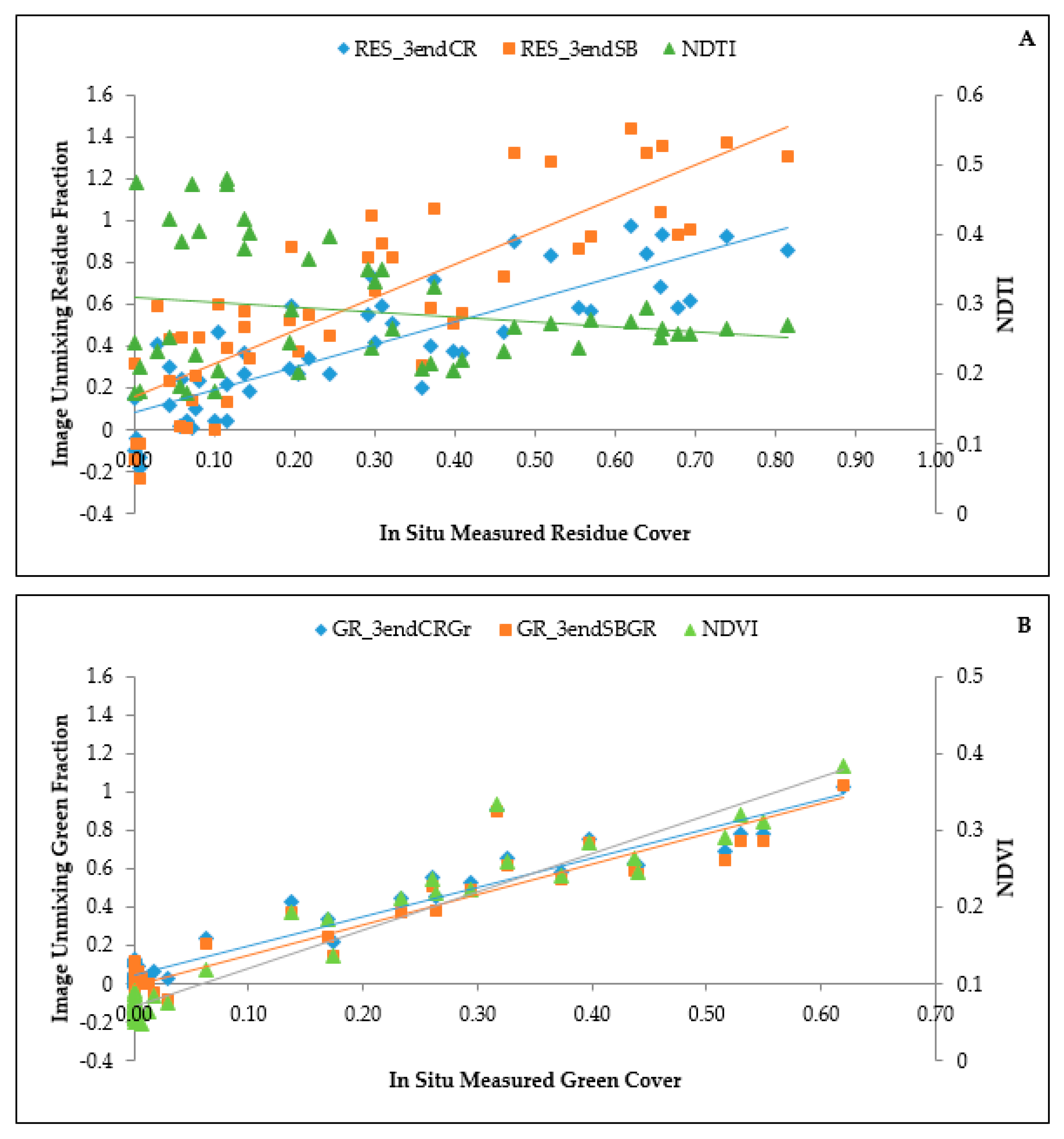
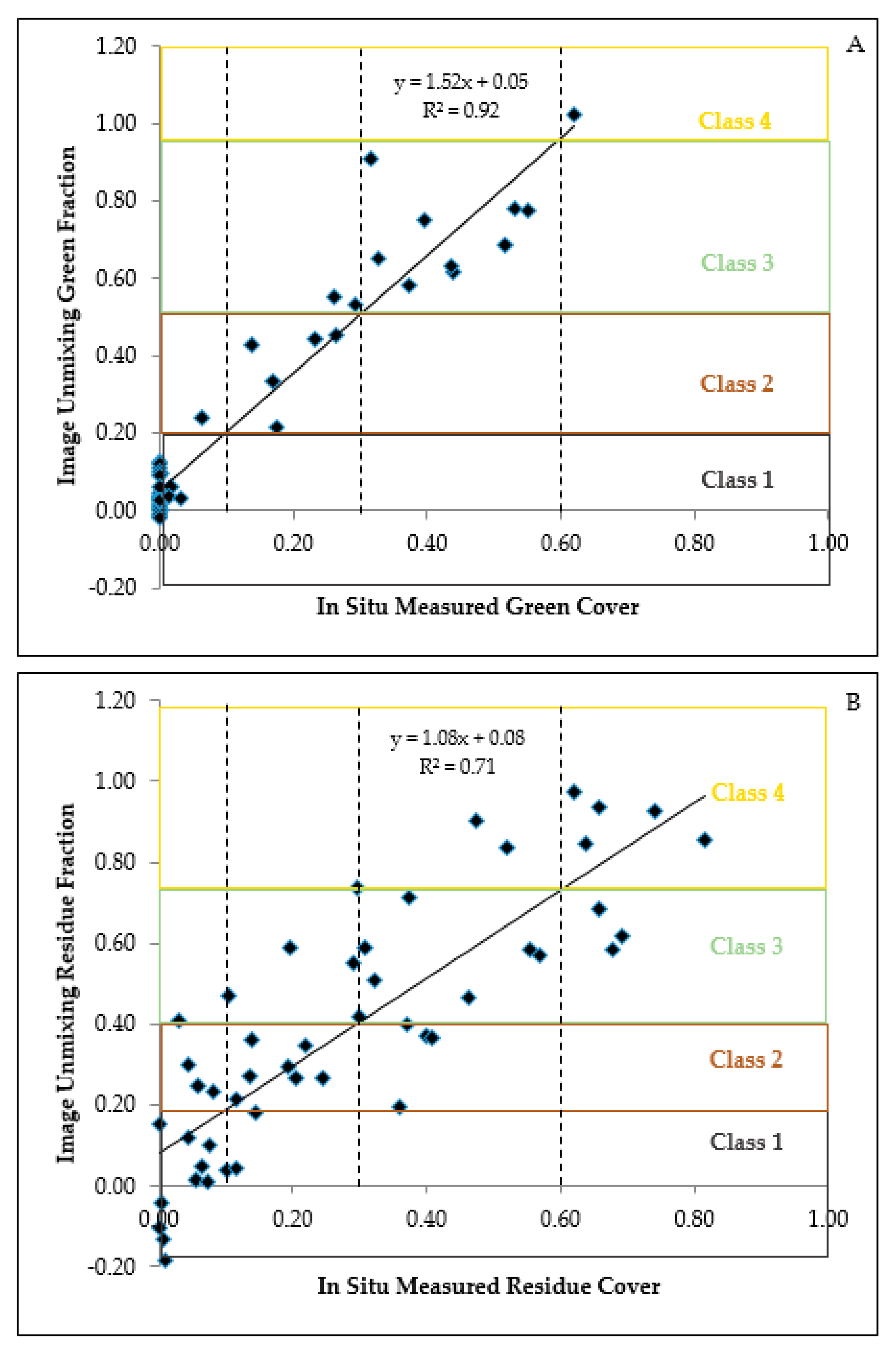
In this paper, accuracy assessments of spectral unmixing data derived from Landsat-8 imagery were made using field data collected during the 2015-2016 post-harvest, pre-planting, and post-planting time periods. The overall accuracies of green and residue covers varied from 77%–95% and 44%–85%, respectively. The analysis indicated that the crop residue type selected for 3 endmember unmixing was not critical; both soybean and corn residue endmembers provided similar and reasonable unmixing results for residue cover and green cover estimates, though which crop endmember had the better fit varied by image and date. It is reasonable to regularly use corn residue as an endmember to avoid having to adjust soybean spectral signatures because of the unlikelihood of finding a 100% pure soybean residue endmember. The results from this study could support the development of operational map products that could be used for performance metrics for the Canada-Ontario Lake Erie Action Plan and as inputs for sustainability indicators that both require knowledge about non-growing season land management over a large area. Soil cover maps of residue and green fractions that have this level of detail are not routinely produced for the Lake Erie Basin, and the spectral signatures generated from this study could be used and validated as baselines for the monitoring of soil cover for other time periods. A thorough study of the spatial patterns of change of soil cover in relation to error levels should be performed to fully assess the advantages and limitations of spectral unmixing for change detection both within and beyond one season.
Overall, spectral unmixing has proved to be cost and time effective. It produced reasonably accurate soil cover classification (e.g., corn and soybean residue cover, green cover and total cover) results of individual imagery and provided a quantitative assessment of the fraction of key selected soil covers in the Canadian Lake Erie basin. However, using satellite imagery to map crop residues showed some limitations possibly due to the inherent difficulties in separating the crop residue spectral signatures from that of soil and the insufficient coverage due to the presence of clouds. Given our relatively large data set of field observations available for model evaluation, further research into the application of nonlinear unmixing approaches should be undertaken [51]. Future work should also benefit from the availability of Sentinel 2A and B satellite images with a revisit time of 5 days, for improving soil cover monitoring. Sentinel 2A and B improved temporal resolution will allow for more frequently available data than Landsat-8 and, therefore, will increase the opportunity for the capture of more optically useful images with minimal cloud cover. This in turn will help in achieving sufficient progress in soil cover mapping, measuring, and estimating spatial variability in crop residue and cover crops over large areas.

Author Contributions

Conceptualization, A.L., P.J., H.M., and A.A.B.; Data curation, A.L, J.H., K.P., and M.B.; Formal analysis, A.L., P.J., A.A.B., J.H., K.P., and M.B.; Funding acquisition, P.J.; Investigation, A.L. and P.J.; Methodology, P.J., H.M., and A.L.; Project administration, P.J.; Supervision, P.J. and H.M.; Validation, K.P., and J.H.; Writing—original draft, A.L. and P.J.; Writing—review & editing of original draft, H.M., A.A.B., J.H., K.P., and M.B.; revising the manuscript according to the academic editor and reviewers’ comments, A.L., P.J., and A.A.B. All the authors have read and agreed to the published version of the manuscript. Dr. Joosse has been designated for handling correspondence at all stages of refereeing and publication as she has received an official invitation to submit this work to a special issue of remote sensing—MDPI journal. All authors have read and agreed to the published version of the manuscript.

Funding

This research was funded in part by Agriculture and Agri-Food Canada Growing Forward 2 funding and Ontario Ministry of Agriculture Food and Rural Affairs, Best Management Practices Verification and Demonstration (BMPVD) funding. The views expressed in this publication are those of the authors and do not necessarily reflect those of the Province of Ontario or the Government of Canada.

Acknowledgments

The authors would like to thank all the farmers for access to their land for this study, Natalie Feisthauer from Agriculture and Agri-Food Canada–STB Guelph, and many students from the Universities of Waterloo and Guelph who assisted with fieldwork and processing the data. Jaison Ambadan from the University of Guelph assisted with creation of some of the plots. Thanks also to Peter Doris and Jennifer Birchmore from OMAFRA for their participation on the project steering committee. We also thank the academic editor and four anonymous reviewers for their helpful comments, which greatly improved earlier versions of the manuscript.

Conflicts of Interest

The authors declare no conflict of interest.

Disclaimer

The use: evaluation and reference to particular products by the authors of this manuscript should not be regarded as an endorsement by AAFC, UM6P, or the University of Guelph.

References

  1. Mailapalli, D.R.; Burger, M.; Horwath, W.R.; Wallender, W.W. Crop residue biomass effects on agricultural runoff. Appl. Environ. Soil Sci. 2013, 2013, 1–8. [Google Scholar] [CrossRef] [Green Version]
  2. Enciso, J.; Nelson, S.D.; Perea, H.; Uddameri, V.; Kannan, N.; Gregory, A. Impact of residue management and subsurface drainage on non-point source pollution in the Arroyo Colorado. Sustain. Water Qual. Ecol. 2014, 3–4, 25–32. [Google Scholar]
  3. Lal, R. Sequestering carbon and increasing productivity by conservation agriculture. J. Soil Water Conserv. 2015, 70, 55A–62A. [Google Scholar] [CrossRef] [Green Version]
  4. Ontario Ministry of Agriculture, Food and Rural Affairs (OMAFRA). New Horizons: Ontario’s Agricultural Soil Health and Conservation Strategy. 2018. Available online: http://www.omafra.gov.on.ca/english/landuse/soil-strategy.pdf (accessed on 31 March 2020).
  5. Canada-Ontario Lake Erie Action Plan. Published by Environment and Climate Change Canada and the Ontario Ministry of the Environment and Climate Change. February 2018. Available online: https://www.canada.ca/content/dam/eccc/documents/pdf/great-lakes-protection/dap/action_plan.pdf (accessed on 31 March 2020).
  6. USDA. Environmental Quality Incentives Program. Natural Resources Conservation Service. Available online: https://www.nrcs.usda.gov/wps/portal/nrcs/main/national/programs/financial/eqip (accessed on 31 March 2020).
  7. Statistics Canada. Table: 32-10-0162-01, Selected Land Management Practices and Tillage Practices Used to Prepare Land for Seeding, Historical Data. Available online: https://doi.org/10.25318/3210016201-eng (accessed on 31 March 2020).
  8. Joosse, P.J.; Baker, D.B. Context for re-evaluating agricultural source phosphorus loadings to the Great Lakes. Can. J. Soil Sci. 2011, 91, 317–327. [Google Scholar] [CrossRef]
  9. Molder, B.; Cockburn, J.; Berg, A.; Lindsay, J.; Woodrow, K. Sediment-assisted nutrient transfer from a small, no-till, tile drained watershed in Southwestern Ontario, Canada. Agric. Water Manag. 2015, 152, 31–40. [Google Scholar] [CrossRef]
  10. Jarvie, H.P.; Johnson, L.T.; Sharpley, A.N.; Smith, D.R.; Bruulsema, T.W.; Confesor, R. Increased soluble phosphorus loads to Lake Erie: Unintended consequences of conservation practices? J. Environ. Qual. 2016, 46, 123–132. [Google Scholar] [CrossRef] [Green Version]
  11. Morrison, J.E., Jr.; Huang, C.H.; Lightle, D.T.; Daughtry, C.S.T. Residue measurement techniques. J. Soil Water Conserv. 1993, 48, 478–483. [Google Scholar]
  12. Dickey, E.C.; Shelton, D.P.; Meyer, G.E.; Fairbanks, K.T. Determining crop residue cover with electronic image analysis. Biol. Syst. Eng. 1989, 238. Available online: https://digitalcommons.unl.edu/biosysengfacpub/238 (accessed on 31 March 2020).
  13. Laamrani, A.; Joosse, P.; Feisthauer, N. Determining the number of measurements required to estimate crop residue cover by different methods. J. Soil Water Conserv. 2017, 72, 471–479. [Google Scholar] [CrossRef] [Green Version]
  14. Laamrani, A.; Pardo Lara, R.; Berg, A.A.; Branson, D.; Joosse, P. Using a Mobile Device “App” and Proximal Remote Sensing Technologies to Assess Soil Cover Fractions on Agricultural Fields. Sensors 2018, 18, 708. [Google Scholar] [CrossRef] [Green Version]
  15. Crop Residue Management Survey (CRM). Conservation Technology Information Centre. 2008. Available online: https://www.ctic.org/resource_display/?id=255 (accessed on 31 March 2020).
  16. Operational Tillage Information System (OpTIS). Available online: https://www.ctic.org/OpTIS (accessed on 31 March 2020).
  17. Mapping Conservation Practices and Outcomes in the Corn Belt. Final Report. Conservation Technology Information Centre, 22 November 2019. Available online: https://www.ctic.org/files/FinalReport_CBPPP_CTIC-TNC_v5.pdf (accessed on 31 March 2020).
  18. Mcnairn, H.; Protz, R. Mapping corn residue cover on agricultural fields in Oxford County, Ontario, using Thematic Mapper. Can. J. Remote Sens. 1993, 19, 152–159. [Google Scholar] [CrossRef]
  19. Daughtry, C.S.T.; Hunt, E.R., Jr.; McMurtrey, J.E., III. Assessing crop residue cover using shortwave infrared reflectance. Remote Sens. Environ. 2004, 90, 126–134. [Google Scholar] [CrossRef]
  20. Sullivan, D.G.; Strickland, T.C.; Masters, M.H. Satellite mapping of conservation tillage adoption in the Little River experimental watershed, Georgia. J. Soil Water Conserv. 2008, 63, 112–119. [Google Scholar] [CrossRef]
  21. Daughtry, C.S.T.; Hunt, E.R., Jr. Mitigating the effects of soil and residue water contents on remotely sensed estimates of crop residue cover. Remote Sens. Environ. 2008, 112, 1647–1657. [Google Scholar] [CrossRef]
  22. Serbin, G.; Hunt, E.R.; Daughtry, C.S.T.; McCarty, G.W.; Doraiswamy, P.C. An improved ASTER index for remote sensing of crop residue. Remote Sens. 2009, 1, 971–991. [Google Scholar] [CrossRef] [Green Version]
  23. Galloza, M.S.; Crawford, M.M.; Heathman, G.C. Crop residue modeling and mapping using Landsat, ALI, Hyperion, airborne remote sensing data. IEEE J. Sel. Top. Appl. 2013, 6, 446–456. [Google Scholar] [CrossRef]
  24. Bannari, A.; Staenz, K.; Champagne, C.; Khurshid, K.S. Spatial variability mapping of crop residue using hyperion (EO-1) hyperspectral data. Remote Sens. 2015, 7, 8107–8127. [Google Scholar] [CrossRef] [Green Version]
  25. Jin, X.; Ma, J.; Wen, Z.; Song, K. Estimation of maize residue cover using Landsat-8 OLI image spectral information and textural features. Remote Sens. 2015, 7, 14559–14575. [Google Scholar] [CrossRef] [Green Version]
  26. Rundquist, S.; Carlson, S. Mapping Cover Crops on Corn and Soybeans in Illinois, Indiana and Iowa, 2015–2016. March 2017. Available online: https://www.agri-pulse.com/ext/resources/pdfs/EWG_CoverCropReport_C05.pdf (accessed on 31 March 2020).
  27. Seifert, C.A.; Azzari, G.; Lobell, D.B. Satellite detection of cover crops and their effects on crop yield in the Midwestern United States. Environ. Res. Lett. 2018, 13, 064033. [Google Scholar] [CrossRef]
  28. Sharma, V.; Irmak, S.; Kilic, A.; Sharma, V.; Gilley, J.E.; Meyer, G.E.; Knezevic, S.Z.; Marx, D. Quantification and Mapping of Surface Residue Cover for Maize and Soybean Fields in South Central Nebraska. Trans. ASABE 2016, 59, 925–939. [Google Scholar]
  29. Pacheco, A.; McNairn, H. Evaluating multispectral remote sensing and spectral unmixing analysis for crop residue mapping. Remote Sens. Environ. 2010, 114, 2219–2228. [Google Scholar] [CrossRef]
  30. Hively, W.D.; Lamb, B.T.; Daughtry, C.S.T.; Shermeyer, J.; McCarty, G.W.; Quemada, M. Mapping Crop Residue and Tillage Intensity Using WorldView-3 Satellite Shortwave Infrared Residue Indices. Remote Sens. 2018, 10, 1657. [Google Scholar] [CrossRef] [Green Version]
  31. Daughtry, C.S.T.; Hunt, E.R.; Doraiswamy, P.C.; McMurtrey, J.E. Remote Sensing the Spatial Distribution of Crop Residues. Agron. J. 2005, 97, 864–871. [Google Scholar] [CrossRef]
  32. Wang, G.; Wang, J.; Zou, X.; Chai, G.; Wu, M.; Wang, Z. Estimating the fractional cover of photosynthetic vegetation, non-photosynthetic vegetation and bare soil from MODIS data: Assessing the applicability of the NDVI-DFI model in the typical Xilingol grasslands. Int. J. Appl. Earth Obs. Geoinf. 2019, 76, 154–166. [Google Scholar] [CrossRef]
  33. Yue, J.; Tian, Q.; Tang, S.; Xu, K.; Zhou, C. A dynamic soil endmember spectrum selection approach for soil and crop residue linear spectral unmixing analysis. Int. J. Appl. Earth Obs. Geoinf. 2019, 78, 306–317. [Google Scholar] [CrossRef]
  34. Sonmez, N.K.; Slater, B. Measuring intensity of tillage and plant residue cover using remote sensing. Eur. J. Remote Sens. 2016, 49, 121–135. [Google Scholar] [CrossRef] [Green Version]
  35. Zheng, B.; Campbell, J.B.; de Beurs, K.M. Remote sensing of crop residue cover using multi-temporal Landsat imagery. Remote Sens. Environ. 2012, 117, 177–183. [Google Scholar] [CrossRef]
  36. Zheng, B.; Campbell, J.B.; Serbin, G.; Daughtry, C.S.T. Multitemporal remote sensing of crop residue cover and tillage practices: A validation of the minNDTI strategy in the United States. J. Soil Water Conserv. 2013, 68, 120–131. [Google Scholar] [CrossRef]
  37. Hively, W.D.; Shermeyer, J.; Lamb, B.T.; Daughtry, C.T.; Quemada, M.; Keppler, J. Mapping Crop Residue by Combining Landsat and WorldView-3 Satellite Imagery. Remote Sens. 2019, 11, 1857. [Google Scholar] [CrossRef] [Green Version]
  38. Schut, L.W. Soils of Elgin County; Agric. Canada Research Branch: Toronto, ON, Canada, 1992. [Google Scholar]
  39. Kludze, H.; Deen, B.; Dutta, A. Report on Literature Review of Agronomic Practices for Energy Crop Production under Ontario Conditions; University of Guelph: Guelph, ON, Canada, 2011; Available online: https://ofa.on.ca/wp-content/uploads/2017/11/OFA-PROJECT-FINAL-REPORT-JULY-04-2011-RAAC1.pdf (accessed on 31 March 2020).
  40. Kludze, H.; Deen, B.; Weersink, A.; van Acker, R.; Janovicek, K.; De Laporte, A.; McDonald, A. Estimating sustainable crop residue removal rates and costs based on soil organic matter dynamics and rotational complexity. Biomass Bioenergy 2013, 56, 607–618. [Google Scholar] [CrossRef]
  41. Environment Canada. Canadian Climate Normals 1971–2000 St. Thomas Weather Station. Government of Canada, 2011. Available online: http://climate.weather.gc.ca/climate_normals (accessed on 18 February 2020).
  42. PCI Geomatica 2015 Software. Richmond Hill, ON, Canada. Available online: https://www.pcigeomatics.com/pressnews/2015_PCI_Geomatica-15.pdf (accessed on 31 March 2020).
  43. Richter, R.; Schläpfer, D. Atmospheric/Topographic Correction for Satellite Imagery; ATCOR-2/3 User Guide, Version 9.0.0; DLR Report DLR-IB; ReSe Applications Schläpfer: Langeggweg, Switzerland, 2015. [Google Scholar]
  44. Boardman, J.M.; Kruse, F.A.; Green, R.O. Mapping target signature via partial unmixing of AVIRIS data. In Summaries of the Fifth JPL Airborne Earth Science Workshop; JPL Publication 95–1; NASA Jet Propulsion Laboratory: Pasadena, CA, USA, 1995; pp. 23–26. [Google Scholar]
  45. ENVI Image Analysis Software; Harris Geospatial Solutions, Inc.: Broomfield, CO, USA; Available online: https://www.harrisgeospatial.com/Software-Technology/ENVI (accessed on 31 March 2020).
  46. Rouse, J.W.; Haas, R.W.; Schell, J.A.; Deering, D.W.; Harlan, J.C. Monitoring vegetation systems in the Great Plains with ERTS. In Third Earth Resources Technology Satellite–1 Syposium; Freden, S.C., Mercanti, E.P., Becker, M., Eds.; Technical Presentations, NASA SP-351; NASA: Washington, DC, USA, 1974; Volume I, pp. 309–317. [Google Scholar]
  47. van Deventer, P.; Ward, D.; Gowda, P.H.M.; Lyon, J.G. Using thematic mapper data to identify contrasting soil plains and tillage practices. Photogramm. Eng. Remote Sens. 1997, 63, 87–93. [Google Scholar]
  48. R Development Core Team. A Language and Environment for Statistical Computing; R Foundation for Statistical Computing: Vienna, Austria; Available online: http://www.r-project.org/ (accessed on 31 March 2020).
  49. Fisk, C.; Clarke, K.D.; Lewis, M.M. Comparison of hyperspectral versus traditional field measurements of fractional ground cover in the Australian arid zone. Remote Sens. 2019, 11, 2825. [Google Scholar] [CrossRef] [Green Version]
  50. Koirala, B.; Khodadadzadeh, M.; Contreras, C.; Zahiri, Z.; Gloaguen, R.; Scheunders, P. A supervised method for nonlinear hyperspectral unmixing. Remote Sens. 2019, 11, 2458. [Google Scholar] [CrossRef] [Green Version]
  51. Fisk, C.; Clarke, K.D.; Delean, S.; Lewis, M.M. Distinguishing photosynthetic and non-photosynthetic vegetation: How do traditional observations and spectral classification compare? Remote Sens. 2019, 11, 2589. [Google Scholar] [CrossRef] [Green Version]
Figure 1. Map of the study area including major cities (black stars) and the Landsat images required to cover the Canadian Lake Erie basin (squares outlined in gray). Numbers in the middle of each image (e.g., 18/30) refer to the Landsat path and row, respectively. The same path indicates same day acquisition (e.g., 19/31 and 19/30).
Remotesensing 12 01397 g001
Figure 2. Examples of the pure endmembers used in this study: corn residue (A), bare soil (B), soybean residue (C), and green cover (D; alfalfa in this case).
Remotesensing 12 01397 g002
Figure 3. Example of ground truthing fields with close up of an area in the Elgin site. Fields representing some of the endmembers used in unmixing are shown with asterix on (A) for the pre-planting 2016-04-18 image (SWIR1 (7), SWIR1 (6), blue (2) in RGB). Resulting unmixed raster images of green cover (B), bare soil (C), and corn residue (D). In each image (BD), fractions vary from 0 to 1, with the highest fractions displayed in white.
Remotesensing 12 01397 g003
Figure 4. Unmixing fraction results using soybean or corn three end member combinations and index results for Image 18/30 2016-04-18 (n = 49). (A) Residue fraction and normalized difference tillage index (NDTI) compared to measured residue cover (B) Green fraction and Normalized Difference Vegetated Index (NDVI) compared to measured green cover.
Remotesensing 12 01397 g004
Figure 5. Illustration of breakpoints in fraction values used to define common soil cover (e.g., green cover (A) or residue (B)) classes. Data from the 18/30 2016-04-18 image (n = 49).
Remotesensing 12 01397 g005
Figure 6. Comparison of total soil cover calculated from linear relationships for separate residue and green cover (Figure 5) and in situ residue and green cover data summed together. Data from the 18/30 2016-04-18 image (n = 49).
Remotesensing 12 01397 g006
Table 1. Acquisition characteristics and spectral bands of the satellite scenes used in the study.
Mission, SensorPath/Row (Area)Spectral Bands 1Spatial Resolution (m)
Band 2 (blue)30
Landsat-818/30 (Elgin)Band 3 (green)30
Operational19/30 (Elgin)Band 4 (red)30
Land Imager20/31 (Essex)Band 5 (NIR)30
(OLI)20/31 (Essex)Band 6 (SWIR1)30
Band 7 (SWIR2)30
1 Bands 1 (Coastal), 8 (Panchromatic), 9 (Cirrus), 10 (TIRS1), and 11 (TIRS2) were not used in this study. NIR = Near-infrared; SWIR = Short Wave Infrared.
Table 2. Dates of Landsat-8 images used to derive soil cover percentage for different periods.
Year/Practice PeriodElginEssex
18/3019/3019/3120/31
2015–2016Post-harvestnd *Nov-1-15Nov-1-15Nov-8-15
Pre-plantingApr-18-16Apr-25-16 ŦApr-16-16
Post-plantingMay-27-16 ŦMay-27-16 ŦMay-18-16
* nd—No ground data were collected due to cloud cover over the investigated area. † Ground data were collected but corresponding imagery was covered by clouds. Ŧ Green cover data collected 3–8 days prior to image acquisition.
Table 3. Endmember combinations used in spectral unmixing and resulting fraction images analyzed.
# of EndmembersInput Endmember CombinationsOutput Fraction Image (Raster)Labels Hereafter
2Corn residue (CR) + Bare soilResidue fraction using CR residue as one of 2 endmembers2EndCR
2Soybean residue (SB) + Bare SoilResidue fraction using SB residue as one of 2 endmembers2EndSB
3CR residue + Bare Soil + Green cover (Gr)Residue fraction using CR residue as one of 3 endmembers3EndCR
Gr fraction using CR residue as one of 3 endmembers3EndCRGr
3SB residue + Bare soil + GrResidue fraction using SB residue as one of 3 endmembers3EndSB
GR fraction using soybean residue as one of 3 endmembers3EndSBGr
4CR residue + SB residue + Bare soil + GrCR residue fraction using 4 endmembers4EndCR
SB residue fraction using 4 endmembers4EndSB
Gr fraction using 4 endmembers4EndGr
Table 4. Summary of unmixing results estimated using 2, 3, and 4 endmember combinations correlated with in situ measured residue or green cover for image 18/30 2016-04-18 (n = 49).
Unmixed Fraction (y) In Situ Measured Soil Cover (x)SlopeInterceptR2RMSE
2EndCRRES0.350.670.030.49
2EndSBRES0.020.830.000.62
3EndCRRES1.080.080.71 †0.16
3EndSBRES1.580.160.72 †0.23
4EndCRRES−1.922.420.061.86
4EndSBRES3.10−2.420.12 *1.97
3EndCRGrGR1.520.050.92 †0.08
3EndSBGrGR1.58−0.010.91 †0.09
4EndGrGR1.660.110.80 †0.15
RES = residue cover of any crop type and GR = green cover of any crop type. R2 = Coefficient of determination. RMSE = root mean squared error. * and † refer to relationships with p-value < 0.05 and <0.001, respectively.
Table 5. Comparison between subsets of field residue cover measurements (x) and unmixed residue fractions (y) for different crop residue type endmembers used in 3 endmember unmixing of image 18/30 2016-04-18.
5a. CR Residue Fraction (3EndCR)nRMSER2InterceptSlope
CR residue, no Gr cover130.130.67 †−0.031.20
SB residue, no Gr cover40.160.490.181.13
Bare, CR, SB, no Gr cover 260.150.80 †0.011.17
All Residue types, no Gr cover280.180.73 †0.051.12
Residue for All Fields 490.170.71 †0.081.08
5b. SB Residue Fraction (3EndSB)
CR residue, no Gr cover 130.190.68 †−0.021.76
SB residue, no Gr cover40.220.580.151.82
Bare, CR, SB, no Gr cover 260.230.80 †0.041.72
All Residue types, no Gr cover 280.240.75 †0.091.66
Residue for All Fields 490.230.72 †0.161.58
n = number of sampling areas used; CR = corn; SB = Soybean; Gr = Green. † refer to relationships with p-value < 0.001.
Table 6. Range (minimum (Min) and maximum (Max) values) and mean of linear regression parameters between unmixing fraction or index values compared to ground truth residue cover (RES) or green cover (GR) measures for nine 2015–2016 non-growing season images cited in Table 2.
RasterR2RMSE
MinMaxMeanMinMaxMean
RES_3endCR0.520.870.700.140.330.21
RES_3endSB0.390.860.700.170.460.26
RES_NDTI0.000.570.160.020.120.05 *
GR_3endCRGr0.760.960.870.060.170.11
GR_3endSBGr0.760.960.870.050.170.11
GR_NDVI0.800.980.890.020.120.05 *
* Note, these are Index values.
Table 7. Breakpoints in fraction values between common soil cover (e.g., residue and/or green cover) classes.
ClassPercentage CoverX for Breakpoints in Linear EquationsInterpretation
1<10% Essentially bare soil
210–30%0.1Inadequate cover for erosion protection
330–60%0.3Conservation tillage, adequate cover
4>60%0.6No-tillage, high cover
Table 8. Individual image accuracy results for linear regression (point fractions) and confusion matrix (fraction classes) for unmixing residue and green cover fractions (using corn residue + green cover + bare soil endmembers) and calculated total cover compared to in situ measures, respectively.
2015–2016 Non-growing SeasonnResidue CoverGreen CoverTotal Cover
RMSEOARMSEOARMSEOA
Post-Harvest_19/30390.270.850.120.900.200.62
Post-Harvest_19/31550.140.730.090.930.110.60
Post-Harvest_20/31430.210.670.060.880.130.72
Pre-Planting_20/31470.160.600.160.870.070.64
Pre-Planting_18/30490.170.590.080.940.150.61
Pre-Planting_19/30460.210.440.140.830.220.48
Post-planting_20/31470.140.810.080.900.120.72
Post-planting_19/30380.290.550.170.770.180.50
Post-planting_19/31550.330.530.110.950.140.46
OA = Overall accuracy calculated from the confusion matrix.

