A Change-Driven Image Foveation Approach for Tracking Plant Phenology
by
 , , and
Ewerton Silva
1, 
Ricardo da S. Torres
2,*,
Bruna Alberton
3,
Leonor Patricia C. Morellato
3 and
Thiago S. F. Silva
4
1
Institute of Computing, University of Campinas, Campinas 13083-852, Brazil
2
Department of ICT and Natural Sciences, Norwegian University of Science and Technology, Larsgårdsvegen 2, 6009 Ålesund, Norway
3
Department of Botany, Institute of Biosciences, São Paulo State University, Rio Claro 13506-900, Brazil
4
Biological and Environmental Sciences, Faculty of Natural Resources, University of Stirling, Stirling FK9 4LA, UK
*
Author to whom correspondence should be addressed.
Remote Sens. 2020, 12(9), 1409; https://doi.org/10.3390/rs12091409
Submission received: 28 March 2020
/
Revised: 23 April 2020
/
Accepted: 26 April 2020
/
Published: 29 April 2020
(This article belongs to the Section Remote Sensing Communications)
Abstract
:One of the challenges in remote phenology studies lies in how to efficiently manage large volumes of data obtained as long-term sequences of high-resolution images. A promising approach is known as image foveation, which is able to reduce the computational resources used (i.e., memory storage) in several applications. In this paper, we propose an image foveation approach towards plant phenology tracking where relevant changes within an image time series guide the creation of foveal models used to resample unseen images. By doing so, images are taken to a space-variant domain where regions vary in resolution according to their contextual relevance for the application. We performed our validation on a dataset of vegetation image sequences previously used in plant phenology studies.

1. Introduction
Vision stands out among other long-evolved biological sensing mechanisms because of its complexity and effectiveness. Unlike conventional digital cameras, the human retina is designed to perceive in a non-uniform manner. While the fovea centralis extracts high-resolution data, the retinal periphery perceives with a gradually-decreasing resolution. By operating with less data and relying on saccades [1], the brain processes these space-variant images more efficiently [2,3]. This scheme has been applied to image-based tasks, such as computer vision [4,5,6,7,8] and image compression [9,10,11].
As a rich source of data, digital images have triggered scientific advances in several areas. In plant phenology, where life cycle events are investigated along with their relationships to climate [12,13], knowledge of plant and vegetation dynamics over time is essential to understand ecosystem processes such as carbon and water exchange [14]. Manual on-the-ground data sampling and investigation can be coupled with hardware/software apparatuses to better capture, manage, and process multimedia data (e.g., images and videos), thus supporting phenological studies in several ways [15]. For the past decades, image-based phenological studies have been successfully developed using satellite-based imaging [16], near-surface cameras [14,15] and more recently, unmanned aerial vehicles [17].
A technical challenge imposed by phenological imaging is related to the memory space occupied, given the need for frequent and extensive imaging. Although hardware technology is continuously advancing in terms of storage capacity, some computing environments still face restrictions on data volumes, such as near real-time data processing applications and bandwidth-limited remote data transfer. For uses such as phenological monitoring, redundancy in image sequences due to invariant or slow-changing pixels contributes largely to the storage issue. Another significant feature of uniform high-resolution images is that they provide detailed data about relevant and non-relevant regions, without distinction, as a result of the underlying acquisition process in traditional cameras. In foveated vision systems, such an issue relates to the task of finding fixation points (i.e., foveal centers) across one or more images, which enables a space-variant image representation to be devised. When applying models of human vision, however, one must be aware of the difficulty in predicting human fixations, as these vary strongly between different subjects and tasks. Thus, as an extra challenge, algorithms to find appropriate fixation points should be application-dependent, as there is no optimal routine that covers all possible vision tasks [18].
Inspired by foveation and human perception, some approaches have attempted to address these challenges. Niu et al. [9] proposed a foveal imaging system comprising a set of lenses and a scanning microlens to produce images where a region is locally magnified and the remaining regions stay unchanged. The authors claim the system is suitable for object tracking and monitoring applications due to its dynamic foveal mechanism. However, peripheral resolution cannot be degraded and different microlenses are necessary to vary the structural foveal arrangement. Shi et al. [10] introduced a foveation-oriented approach to compress remote sensing images in which good image quality levels can be retained for inspection tasks. Nonetheless, such a study only considers a central fovea, and different fixation points are not investigated, which could be convenient in real scenarios. Bektas et al. [11] took human perception concepts into account to compress geographical images in a perceptually lossless manner. By applying models of visual perception, the approach favored data reduction and user experience in tasks involving visual interpretation of images. The study conducted experiments with real users that had their eye’s tracked while performing searching tasks in a sequence of images. The results showed that few participants noticed the degradation artifacts caused by processing the images with the models. However, the participants were only assigned the task of looking for a circular map symbol in each image, therefore not delving into specific tasks such as identifying and recognizing places, structures, and other contextual elements.
The interesting balance between efficiency and resource allocation provided by foveal images has led us to further explore this idea. Here, we demonstrate an image representation approach that resembles the human retina in plant phenology tracking. Our method combines segmentation and image foveation to create foveal models and images with varying degrees of spatial resolution. Such variation depends on a contextual relevance that, in our validation scope, is determined by a phenological metric and a behavior pattern of choice. We show that our models yield storage savings, while also retaining efficiency in commonly adopted settings of the phenology research field.
This paper is organized as follows. Section 2 describes our approach for devising image models based on a change-driven strategy and on foveation concepts. Section 3 shows the adopted dataset, as well as the steps needed to create the models and to reconstruct images on top of these models. Section 4 presents experimental details regarding the validation steps, shows the results, and discuss them. Section 5 concludes the paper and highlights topics for further investigation.
2. Proposed Approach
Figure 1 shows the complete workflow of our approach. First, a set of images captured over a time period is used for training. Then, the following steps are performed:
- Binary Map: This step creates a binary map encoding a phenological event, and segments the image space into foveal and peripheral regions. For such, we employ a motion history histogram (MHH) [19] to create a frequency map representing the spatial occurrence of binary behavior patterns over a sequence of binary change maps (CM). A CM encodes a desired change, which is determined by a phenological metric, between two RGB images. For instance, the metric of Increase (Equation (1)) can be used to encode a Green-up event by capturing increases in the green-channel pixel values (leaves) of a certain plant individual over time.In Equation (1), stands for the change map of two consecutive images from the sequence (the first one at timestamp t), and refers to the -pixel value in the t-th image. Note that a sequence of N images yields CMs.The successful use of CMs to depict changes on plant phenology was developed and tested using data derived from ground-based direct visual observation, and relying on MHHs to detect and represent temporal changes in arbitrary temporal multivariate numerical data [20]. Here, we applied the proposed binary encoding approach to characterize phenological events. The MHH stores the frequency each pixel featured a specific behavior in the CM sequence. For instance, a “short” Increase behavior can be modeled as 0110, which refers to an increase of the values of a specific pixel in two consecutive images. Figure 2 exemplifies the idea of detecting binary patterns in a series of typical phenological images. However, we use a binarized version of MHH as we are only interested in pixel positions where a pattern was detected with a frequency greater than a threshold sigma (). Figure 3 illustrates the complete process.
- Gaussian Kernel Density Estimation (KDE): After delineating foveal and peripheral regions, the next step estimates a 2-d non-parametric probability density function from the binary map using a KDE. The final artifact of this process is a 2-d real-valued matrix representing the corresponding function and matching the size of the map. However, as an inverse analogy to the distribution of cones in the retina, we adjusted the function such that its values increase with the distance to the fovea(s), thus resembling an upside-down 2-d mixture of Gaussians. In Figure 1, the red and blue regions indicate high and low values, respectively.
- Foveal Model: We used the non-parametric function and a Hilbert curve in a pixel-sampling procedure to create a foveal model. The Hilbert curve maps a 1-d parameter space to a higher-dimensional space (i.e., 2-d), thus creating a sequential order by visiting each midpoint of a square once. Unlike a usual raster-scan approach, the Hilbert curve favors the preservation of locality properties inherent in multidimensional data, as it traverses neighboring regions prior to visiting distant ones [21].The proposed method initially divides the image space into four squares around its center. Given that the Euclidean distances of the square’s midpoint to its two closest neighbors are greater than the value of the non-parametric function at the midpoint, each square is then recursively divided into four equal-sized squares. This can be envisioned as a gradual refinement process in which more pixels are sampled the closer these are to a fovea. The stop condition occurs when trying to reach subpixel positions, when a square is not refined any further. The final curve is not homogeneous (see Figure 1), with its vertices constituting the non-uniform sampling scheme.
- Space-Variant Region of Interest (sROI): Although the foveal model may contain regions of variable interest, one might choose only a subset of them. Having a gradually-decreasing resolution from the foveal centers towards peripheral regions could be helpful in specific circumstances. Instead of using a delimiting rectangular window or a binary mask over a uniform image, a space-variant model allows us to deal with a non-uniformly constrained region of interest, which we refer hereafter as sROI, that may represent a phenological behavior of a given plant individual over time.
After a “training” step, a new set of images taken in a different time period but from the same area can be used to test the foveal models and their extracted sROIs. Images can be taken as a set of sparse points, or be reconstructed by several methods (e.g., voronoi diagrams, quad-trees) that provide a 2-d space-variant representation. From that, data can be extracted and processed (e.g., phenological visual rhythms and interest-point/statistical descriptors). By using space-variant images, memory storage may be reduced given some image are represented at different resolutions and contain less data.
3. Materials and Methods
In this section, we detail the experimental procedure adopted, including the dataset used, how foveal models are generated, and the image reconstruction (or resampling) step.
3.1. Dataset
The dataset employed contains daily sequences of RGB images (in JPEG format) with pixels. The sequence covers the years from 2012 to 2015: where, everyday, an average of six images were captured for every hour (between 6 am to 6 pm). Binary masks of field-identified individual plants are also available. The images were produced with a digital hemispherical lens camera (Mobotix Q 24, Mobotix AG—Germany), which was placed on a monitoring tower far above the canopy and recorded the phenology of a Cerrado (neotropical savanna) area at Itirapina, São Paulo, Brazil [15,22]. Our study occurred during the transition between the dry and the wet season, a period when most of the plant species are producing new leaves. According to [22], in which a dataset from the same area was used, leaf flush periods occur from the end of August to the beginning of October. Thus, for most experiments, we considered the day of the year (DOY) ranging between 241 and 273. The sunrise, sunset, and solar elevation angle were 6:23 h, 18:01 h, 47.2° (DOY 241), and 05:52 h, 18:10 h, 59° (DOY 273), respectively.
3.2. Foveal Models
To generate the models, we used the 2012 image dataset, which was preprocessed as follows. First, we removed unwanted elements, such as the camera tower and the information inserted by the camera’s software. Then, images were down-scaled to 25% of their original size ( pixels) to favor the creation of well-structured models (i.e., with a few, smooth foveal regions). Using scale-space inspections, enabled with gaussian pyramid decompositions, we noticed that images at lower scale levels (i.e., with reduced sizes) provide more satisfactory models, as it removes most noise-like data. Each image was then converted into its green chromatic coordinate (GCC) representation. The GCC is a common index used for near-surface phenology that reflects a measurement of the proportion of green color signal on an RGB image pixel or region [15,22,23]. Finally, we calculated the 90th percentile of each day to encapsulate relevant daily data into a single image and, possibly, minimize the impact of lighting changes (e.g., intensity, angles) on the time series [23].
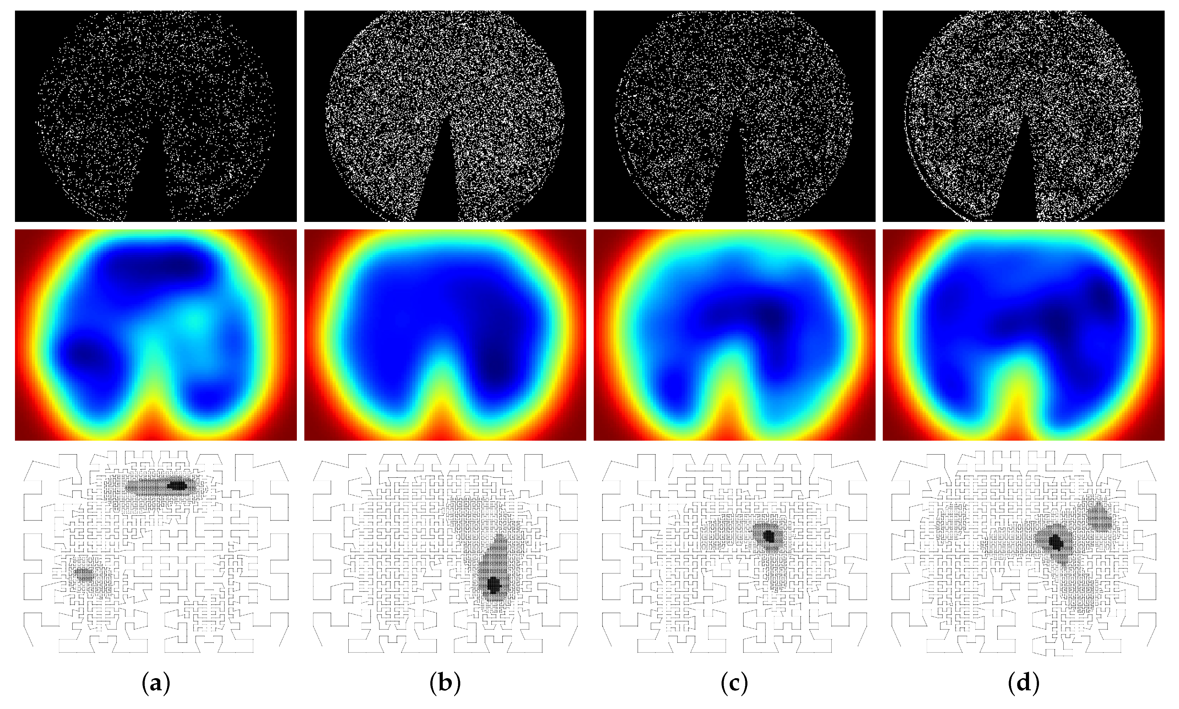
We selected four binary patterns typifying different behaviors of a phenological change of Increase (see Section 2) encoded in MHHs. The 010, 0110, 01110, and 011110 patterns (ordered from the shortest to the longest) indicate how pixels behave in terms of frequencies of continuous changes (sequences of “1”s) bounded by steady states (bordering “0”s) throughout the image series. Although other temporal patterns could be contemplated, we have chosen these because, together with the Increase metric, they are capable of encoding the Green-up change. For each pattern, we used different values of sigma (; found empirically) to binarize the MHHs. Finally, the models generated (i.e., their points) were re-scaled back to the original, high-resolution size. Figure 4 shows the MHHs, KDE implicit functions, and foveal models generated for each pattern. The “spreading” aspect of MHHs also allows us to identify all regions that respond to a particular event.
3.3. Image Reconstruction
A plausible approach consists in returning to the 2-d space by means of a reconstruction step. When doing this, the image is essentially uniform, but its contents get represented in a space-variant domain. Figure 5 illustrates the procedure we adopted in this paper, which relies on calculating a voronoi diagram for the set of points comprising each model, then reconstructing the image by drawing voronoi cells filled with the same RGB color of the cell’s central pixel in the captured scene. This creates a foveal image that has greater content heterogeneity in foveal regions, as these carry higher resolutions compared to peripheral ones.
4. Results
In this section, we present a validation for the proposed workflow. We assess the effectiveness of foveal models in terms of time series’ correlation rates of an appropriate vegetation index and memory storage usage induced by models.
4.1. Evaluation for Reconstructed Images and ROIs
In plant phenology, monitoring variations in plant individual features, such as those related to color and shape, are paramount to understand the phenophases that these individuals undergo, and, consequently, the associated ecosystem processes [15]. A suitable measure to determine these variations in digital images over time is the mean GCC of image pixels or regions. Thus, we validated the foveal models from Section 3.2 by comparing regions from original and reconstructed images having plant individuals known to undergo the same phenological change (i.e., Increase) encoded in the models. We used individuals of the Aspidosperma tomentosum and Caryocar brasiliensis species (for details see [22]).
We tested the models with high-resolution images from the years of 2013, 2014, and 2015. The top panels of Figure 6-top show the mean GCC time series regarding the tested years for original and foveal images with each model. To measure the similarity between the original and foveal time series, we calculated the Pearson Correlation value between series (Figure 6-bottom panels). The high positive correlation results suggest that the reconstructed visual information is still significant even under varying resolution and degradation levels caused by the space-variant representation. Additionally, models encoding the 010 and 0110 patterns seem more effective at incorporating visual information from Aspidosperma tomentosum individuals, whereas the 011110 pattern is more effective for Caryocar brasiliensis. Figure 7 presents examples of the phenological images used in the experiments, and their masked, reconstructed, and mask-reconstructed versions for a visual inspection.
We also conducted image quality evaluations. Table 1 shows the root mean squared error (RMSE), mean absolute error (MAE), structural similarity index (SSIM), and peak signal-to-noise ratio (PSNR) results for reconstructed images using each model (binary pattern). PSNR and SSIM are two image quality metrics commonly used in the literature to compare different image compression/reconstruction schemes. The PSNR is calculated as the signal peak divided by the strength of the noise, whereas the SSIM quantifies (in the range) the similarity between two images by considering perceptual differences, which include the structural divergences between the depicted objects (e.g., along their edges) caused by image degradation [24]. As expected, SSIM and PSNR values are low, due to the large voronoi cells in peripheral areas. However, RMSE and MAE values were acceptable, indicating that the degradation, although severe in some regions, does not shift the error rates too much, thereby suggesting that foveal images may still be accurate for some analyses, such as plant phenology tracking (as shown in the present study).
4.2. Evaluation for sROIs
Instead of image reconstructions, a subset of the 1-d points from a Hilbert curve can be used. The curve embedded in each foveal model is non-homogeneous and presents variable point densities across the 2-d space it fills. By considering the curve as a sequence of points, such variability can also be verified, but it is necessary to know the refinement level each point in the sequence belongs to. In essence, a new refinement level is obtained every time a recursive call is performed during the model generation (see the algorithmic description in Section 2—step 3), thereby dividing a square area (at the n-th level) into four equal-sized squares, each of which will then belong to the -th level. Points at lower levels are associated with poorly refined regions and coarser resolutions, while points at higher levels are associated with deeper refinements and finer resolutions. In this vein, we introduce the concept of minimum refinement levels (MRLs) to constrain a sequence to a subset comprising all points at and above a certain desired level. We also refer to this MRL-constrained sequence as sROI. In Figure 8, we use (i) different colors to represent distinct refinement levels and (ii) a quad-tree layout we believe is convenient for visualizing the refinement steps leading to the non-homogeneous aspect of the curve. For instance, the 6th MRL includes points at the 6th, 7th, and 8th refinement levels.
The neighborhood preservation property of the Hilbert curve allows us to compare mean GCC correlations from ROIs and sROIs directly. The ROI, in this case, refers to the binary masks of each individual provided by the dataset. Figure 9 shows time series and correlation values for sROIs at the 6th and 8th MRLs of each model. Since sROIs enclose many regions conforming to the event encoded in their models, low correlation values are expected (Figure 9—bottom panels). Moreover, the correlation analyses showed a reverse behavior of some models across distinct species. For example, in the 2013 data, the 010 pattern is positively correlated with Aspidosperma tomentosum, but negatively correlated with Caryocar brasiliensis.
4.3. Storage Usage
A benefit of adopting space-variant image representations is the reduced data volumes. First, our image reconstruction process essentially compresses the images in a space-variant manner. Thus, it is enough to compare the size of these images with the ones obtained with other compression methods. We compared the original image, JPEG images with five quality factors varying from 90 (best) to 10 (worst), and the four foveal models from Section 3 (Figure 10). Our foveal models generated resampled-image sizes that are similar to those obtained via more aggressive JPEG compression actions, i.e., by applying qualities 30 and 10. Additionally, there is a significant difference between the image sizes obtained with our foveal models and with JPEG quality factors above 30, which produce images with less degradation at the cost of higher storage sizes. In contrast, we observed a reduction of around 99% in the number of points (pixels) for the images generated from the foveal models in comparison to the original image (Table 2). The same holds for bytes.
Compared to ROIs and sROIs, the voronoi reconstruction leads to a higher impact on memory storage rates, since more data is required to represent a foveal image in a 2-d uniform cartesian grid. However, as foveal images show greater visual homogeneity in peripheral regions—due to large super-pixel-like artifacts (i.e., voronoi cells)—additional standard compression techniques can also be applied to decrease the storage sizes even further. Moreover, there is no need to save voronoi cells’ vertices, as these can be calculated by voronoi algorithms, but this may require extra and repetitive computational processing. Finally, the combined results of Table 2 and Section 4.2 suggest that the usage of full or MRL-constrained sROIs in phenology tracking (as substitutes for 2-d images) is a valid and viable approach that aims to reduce the manipulated data sizes.
5. Conclusions
We have introduced a change-driven image foveation approach to deal with large volumes of data from phenological images. Several phenology applications must be aware of storage limitations, such as real-time expert processing systems, very-high-resolution imaging sensors, and low-bandwidth remote data transmission. As global long-term and widespread databases of phenological imaging become available, efficient storage with minimal loss will be necessary. To solve these problems, we propose to create foveal models that are able to encode phenological metrics and a behavior pattern. MHHs and a Hilbert curve provide the fixation points/regions and the varying-resolution aspect of the models, respectively. We then propose that these models be applied to create foveal images having less, but also most of the relevant data.
We evaluated model correlation rates for mean GCC time series (2-d and 1-d scenarios), visual quality, and memory storage. Our results show a reduction in the amount of stored data and a viable new image representation, both in terms of quality and relevant-data preservation. In the image compression spectrum, our approach is also valuable as it reaches similar image storage sizes to those obtained with a simple JPEG compression technique using low-quality factors. Although the compressed images show visual artifacts, our compression proceeds in a semantics-wise manner as determined and encoded by the foveal models.
Data variability may represent a challenge to any remote sensing approach targeting vegetation tracking, and we have employed foveation precisely to account for such variation. Although our foveal models may be static and built on top of the behavior seen in a specific year, their resolution-degrading configuration still correlates well with those from subsequent years. For a very long time series, however, our approach might have some natural drawbacks, as climate and anthropogenic issues contribute to amplify uncertainties over time. We leave this investigation for future works.
Finally, examining space-variant imaging sensors and Field Programmable Gate Array devices that are able to handle foveation at the hardware level are promising research venues, as these could boost the autonomy of the image acquisition process, particularly in remote areas. In this context, evaluating energy consumption levels of different foveation procedures, performed on variable hardware and software platforms, could be interesting goals for future studies.
Author Contributions
E.S., R.d.S.T., and T.S.F.S. conceptualized the study and worked on the methodology. E.S. developed the proper software and conducted the majority of the writing, drafting, and production of data visualizations for the paper, being extensively supported by R.d.S.T., T.S.F.S., B.A., and L.P.C.M., which also contributed to the writing, review, and editing process. R.d.S.T., T.S.F.S., B.A., and L.P.C.M. provided the main data resources for allowing the investigation. B.A. and L.P.C.M. worked on the data curation process. All authors were involved in the validation process: E.S. performed the proper validation and, along with R.d.S.T. and T.S.F.S., discussed the relevance of the study to the computing and remote sensing fields, whereas B.A., and L.P.C.M. performed examinations of the results regarding the plant phenology field. Finally, R.d.S.T., L.P.C.M., and T.S.F.S. supervized and administrated all steps of the study, being also responsible for the funding acquisition. All authors have read and agreed to the published version of the manuscript.
Funding
This research was funded by CNPq (grants #307560/2016-3, #311820/2018-2, and #310144/2015-9), São Paulo Research Foundation—FAPESP (grants #2014/12236-1, #2014/00215-0, #2015/24494-8, #2016/50250-1, #2016/01413-5, and #2017/20945-0) and the FAPESP-Microsoft Virtual Institute (grants #2013/50155-0 and #2014/50715-9). This study was financed in part by the Coordenação de Aperfeiçoamento de Pessoal de Nível Superior—Brasil (CAPES)—Finance Code 001.
Conflicts of Interest
The authors declare no conflict of interest.
References
- Zhao, M.; Gersch, T.M.; Schnitzer, B.S.; Dosher, B.A.; Kowler, E. Eye movements and attention: The role of pre-saccadic shifts of attention in perception, memory and the control of saccades. Vis. Res. 2012, 74, 40–60. [Google Scholar] [CrossRef] [PubMed] [Green Version]
- Wandell, B.A. Foundations of Vision; Sinauer Associates, Incorporated: Sunderland, MA, USA, 1995. [Google Scholar]
- Bolduc, M.; Levine, M.D. A Review of Biologically Motivated Space-Variant Data Reduction Models for Robotic Vision. Comput. Vis. Image Underst. 1998, 69, 170–184. [Google Scholar] [CrossRef] [Green Version]
- Jurie, F. A new log-polar mapping for space variant imaging. Pattern Recognit. 1999, 32, 865–875. [Google Scholar] [CrossRef]
- Traver, J.V.; Bernardino, A.; Moreno, P.; Santos-Victor, J. Appearance-Based Object Detection in Space-Variant Images: A Multi-model Approach. In Image Analysis and Recognition: ICIAR 2004; Springer: Berlin/Heidelberg, Germany, 2004; pp. 538–546. [Google Scholar]
- Traver, V.J.; Bernardino, A. A review of log-polar imaging for visual perception in robotics. Robot. Auton. Syst. 2010, 58, 378–398. [Google Scholar] [CrossRef]
- Scassellati, B. Eye Finding via Face Detection for a Foveated, Active Vision System. In Proceedings of the Fifteenth National/Tenth Conference on Artificial Intelligence/Innovative Applications of Artificial Intelligence, American Association for Artificial Intelligence (AAAI ’98/IAAI ’98), Madison, WI, USA, 27–29 July 1998; pp. 969–976. [Google Scholar]
- Pardo, F.; Llorens, I.; Micó, F.; Boluda, J.A. Space variant vision and pipelined architecture for time to impact computation. In Proceedings of the 5th International Workshop on Computer Architectures for Machine Perception, Padova, Italy, 11–13 September 2000; pp. 122–126. [Google Scholar]
- Niu, Y.; Chang, J.; Lv, F.; Shen, B.; Chen, W. Low-cost dynamic real-time foveated imager. Appl. Opt. 2017, 56, 7915–7920. [Google Scholar] [CrossRef] [PubMed]
- Shi, C.; Zhang, J.; Zhang, Y. A Novel Vision-Based Adaptive Scanning for the Compression of Remote Sensing Images. IEEE Trans. Geosci. Remote Sens. 2016, 54, 1336–1348. [Google Scholar] [CrossRef]
- Bektas, K.; Cöltekin, A.; Krüger, J.; Duchowski, A.T. A Testbed Combining Visual Perception Models for Geographic Gaze Contingent Displays; Bertini, E., Kennedy, J., Puppo, E., Eds.; Eurographics Conference on Visualization (EuroVis)—Short Papers; The Eurographics Association: Norrköping, Sweden, 2015. [Google Scholar] [CrossRef]
- Morellato, L.P.C.; Alberton, B.; Alvarado, S.T.; Borges, B.; Buisson, E.; Camargo, M.G.G.; Cancian, L.F.; Carstensen, D.W.; Escobar, D.F.; Leite, P.T.; et al. Linking plant phenology to conservation biology. Biol. Conserv. 2016, 195, 60–72. [Google Scholar] [CrossRef] [Green Version]
- Schwartz, M.D. Phenology: An Integrative Environmental Science; Springer: Berlin, Germany, 2013. [Google Scholar]
- Richardson, A.D.; Braswell, B.H.; Hollinger, D.Y.; Jenkins, J.P.; Ollinger, S.V. Near-surface remote sensing of spatial and temporal variation in canopy phenology. Ecol. Appl. 2009, 19, 1417–1428. [Google Scholar] [CrossRef] [PubMed]
- Alberton, B.; da S. Torres, R.; Cancian, L.F.; Borges, B.D.; Almeida, J.; Mariano, G.C.; dos Santos, J.; Morellato, L.P.C. Introducing digital cameras to monitor plant phenology in the tropics: Applications for conservation. Perspect. Ecol. Conserv. 2017, 15, 82–90. [Google Scholar] [CrossRef]
- Reed, B.C.; Schwartz, M.D.; Xiao, X. Remote Sensing Phenology: Status and the Way Forward. In Phenology of Ecosystem Processes; Noormets, A., Ed.; Springer: New York, NY, USA, 2009; pp. 231–246. [Google Scholar] [CrossRef]
- Klosterman, S.; Melaas, E.; Wang, J.A.; Martinez, A.; Frederick, S.; O’Keefe, J.; Orwig, D.A.; Wang, Z.; Sun, Q.; Schaaf, C.; et al. Fine-scale perspectives on landscape phenology from unmanned aerial vehicle (UAV) photography. Agric. For. Meteorol. 2018, 248, 397–407. [Google Scholar] [CrossRef]
- Floren, A.; Bovik, A.C. Chapter 14—Foveated Image and Video Processing and Search. In Academic Press Library in Signal Processing; Trussell, J., Srivastava, A., Roy-Chowdhury, A.K., Srivastava, A., Naylor, P.A., Chellappa, R., Theodoridis, S., Eds.; Elsevier: Amsterdam, The Netherlands, 2014; Volume 4, pp. 349–401. [Google Scholar]
- Meng, H.; Pears, N.; Freeman, M.; Bailey, C. Motion History Histograms for Human Action Recognition. In Embedded Computer Vision; Kisačanin, B., Bhattacharyya, S.S., Chai, S., Eds.; Springer: London, UK, 2009; pp. 139–162. [Google Scholar]
- Mariano, G.C.; Soares, N.C.; Morellato, L.P.C.; Torres, R.D.S. Change Frequency Heatmaps for Temporal Multivariate Phenological Data Analysis. In Proceedings of the 2017 IEEE 13th International Conference on e-Science (e-Science), Auckland, New Zealand, 24–27 October 2017; pp. 305–314. [Google Scholar]
- Bader, M. Space-Filling Curves: An Introduction with Applications in Scientific Computing, 1st ed.; Springer: Berlin, Germany, 2013; Volume 1. [Google Scholar]
- Alberton, B.; Almeida, J.; Helm, R.; Torres, R.D.S.; Menzel, A.; Morellato, L.P.C. Using phenological cameras to track the green up in a cerrado savanna and its on-the-ground validation. Ecol. Inform. 2014, 19, 62–70. [Google Scholar] [CrossRef]
- Sonnentag, O.; Hufkens, K.; Teshera-Sterne, C.; Young, A.M.; Friedl, M.; Braswell, B.H.; Milliman, T.; O’Keefe, J.; Richardson, A.D. Digital repeat photography for phenological research in forest ecosystems. Agric. For. Meteorol. 2012, 152, 159–177. [Google Scholar] [CrossRef]
- Wang, Z.; Bovik, A.C.; Sheikh, H.R.; Simoncelli, E.P. Image quality assessment: From error visibility to structural similarity. IEEE Trans. Image Process. 2004, 13, 600–612. [Google Scholar] [CrossRef] [PubMed] [Green Version]
Figure 1.
Proposed workflow to generate foveal models and resample phenological images.

Figure 2.
Example of the detection of the 010 and 0110 binary patterns using a series of typical phenological images. Both sides of the figure show the same image series and zoomed-in regions (i.e., the same location in each image). For illustration purposes, the analysis is done only for two pixels from the focused region. Nevertheless, the complete procedure requires the analysis of all image pixels.

Figure 3.
Pipeline of the Binarized MHH generation. This example illustrates the entire process applied to detect a specific pattern throughout the image series. First, two consecutive images and from an image series are compared according to a phenological metric (in this example, the pixel Increase). The comparison yields a binary change map spotting out the pixels that conform to the metric. As comparisons proceed (i.e., as i increases) all change maps (CMs) are inspected towards detecting pixels that change according to a behavior pattern (in this example, 010). Finally, the MHH is gradually updated upon detections. Suppose a pixel at position is found to follow the desired pattern (in this example, green border cells) at a certain point of the examinations. In such a case, would increase by one. After the entire time series has been processed, the MHH is binarized by means of a predefined threshold sigma ().

Figure 4.
MHHs (top), Kernel Density Estimation (KDE) implicit functions (middle), and foveal models (bottom) generated for the (a) 010, (b) 0110, (c) 01110, and (d) 011110 patterns considering the 2012 images.
Figure 4.
MHHs (top), Kernel Density Estimation (KDE) implicit functions (middle), and foveal models (bottom) generated for the (a) 010, (b) 0110, (c) 01110, and (d) 011110 patterns considering the 2012 images.

Figure 5.
Example of image reconstruction. The original image (left) is reconstructed (right) using a voronoi diagram (middle) obtained from a model. Each voronoi cell is filled, in the right image, with the same RGB color of the cell’s central pixel in the left image.
Figure 5.
Example of image reconstruction. The original image (left) is reconstructed (right) using a voronoi diagram (middle) obtained from a model. Each voronoi cell is filled, in the right image, with the same RGB color of the cell’s central pixel in the left image.

Figure 6.
Mean green chromatic coordinate (GCC) time series and correlation results for Aspidosperma tomentosum and Caryocar brasiliensis individuals, considering original and foveal images with each model.
Figure 6.
Mean green chromatic coordinate (GCC) time series and correlation results for Aspidosperma tomentosum and Caryocar brasiliensis individuals, considering original and foveal images with each model.

Figure 7.
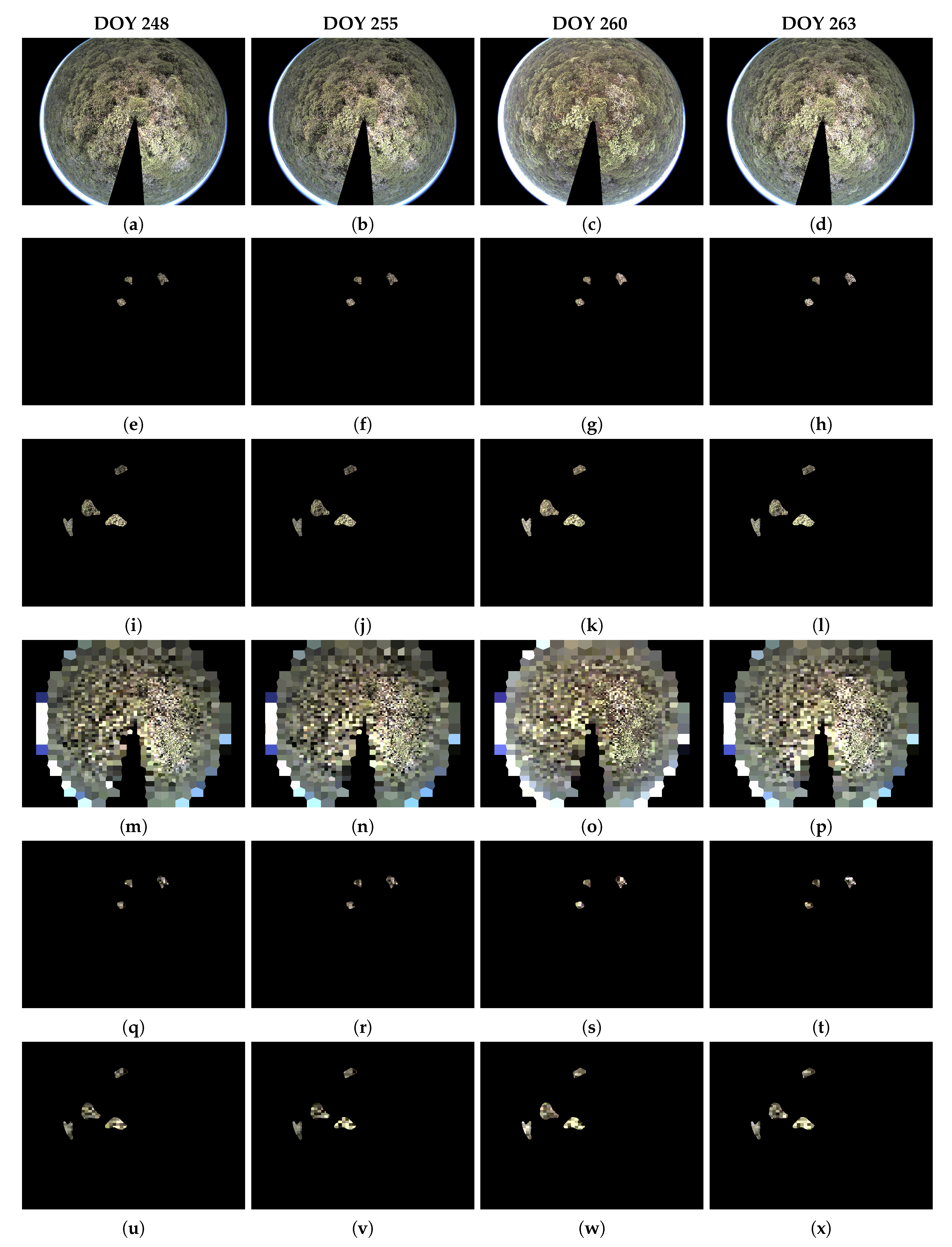
Examples of phenological images from 2013. The days of the year (DOYs) 248, 255, 260, and 263 are column-wise organized. Each row depicts the following: (a–d) original images; masked images containing only the (e–h) Aspidosperma tomentosum and (i–l) Caryocar brasiliensis individuals; (m–p) images reconstructed with the model for the 0110 pattern; and masked-reconstructed images containing only the (q–t) Aspidosperma tomentosum and (u–x) Caryocar brasiliensis individuals.
Figure 7.
Examples of phenological images from 2013. The days of the year (DOYs) 248, 255, 260, and 263 are column-wise organized. Each row depicts the following: (a–d) original images; masked images containing only the (e–h) Aspidosperma tomentosum and (i–l) Caryocar brasiliensis individuals; (m–p) images reconstructed with the model for the 0110 pattern; and masked-reconstructed images containing only the (q–t) Aspidosperma tomentosum and (u–x) Caryocar brasiliensis individuals.

Figure 8.
Space-Variant Region of Interest (sROI) in a quad-tree scheme at the 2nd (left), 6th (middle), and 8th (right) minimum refinement levels (MRLs). Each level is represented in a distinct color. In this case, the lowest MRL is the 2nd, meaning that at least two recursive refinements were performed for any of the four points of the initial curve. The 2nd MRL therefore includes all points of the model. Nevertheless, the highest refinement level of the depicted model is the 8th one. Thus, the 6th MRL comprises the points at the 6th, 7th, and 8th refinement levels, whereas the 8th MRL includes only the points of its own level.

Figure 9.
Mean GCC time series and correlation results for ROIs and sROIs at the 6th and 8th MRLs. Both Aspidosperma tomentosum and Caryocar brasiliensis plant species were considered.
Figure 9.
Mean GCC time series and correlation results for ROIs and sROIs at the 6th and 8th MRLs. Both Aspidosperma tomentosum and Caryocar brasiliensis plant species were considered.

Figure 10.
Comparison of the storage sizes (in kilobytes, KB) of compressed images with our change-driven approach and with the usual JPEG compression process. The models evaluated were the ones generated by the 010, 0110, 01110, and 011110 binary patterns, whereas the JPEG quality factors considered were 10, 30, 50, 70, and 90. The graph shows the mean size of the compressed images.


Table 1.
Results for reconstructed images using the four models respective to the 010, 0110, 01110, and 011110 binary patterns. The considered metrics are root mean squared error (RMSE), mean absolute error (MAE), structural similarity index (SSIM), and peak signal-to-noise ratio (PSNR).
Table 1.
Results for reconstructed images using the four models respective to the 010, 0110, 01110, and 011110 binary patterns. The considered metrics are root mean squared error (RMSE), mean absolute error (MAE), structural similarity index (SSIM), and peak signal-to-noise ratio (PSNR).
| Metric/Pattern | 010 | 0110 | 01110 | 011110 |
|---|---|---|---|---|
| RMSE | 0.2532 | 0.2493 | 0.2509 | 0.2414 |
| MAE | 0.1580 | 0.1555 | 0.1570 | 0.1508 |
| SSIM | 0.3837 | 0.3862 | 0.3836 | 0.3833 |
| PSNR | 11.9327 | 12.0676 | 12.0135 | 12.3479 |
Table 2.
Storage results for full models and sROIs at the 6th-MRL, which includes regions at the 6th, 7th, and 8th refinement levels.
Table 2.
Storage results for full models and sROIs at the 6th-MRL, which includes regions at the 6th, 7th, and 8th refinement levels.
| Storage Results | 010 | 0110 | 01110 | 011110 | ||||
|---|---|---|---|---|---|---|---|---|
| Full | sROI | Full | sROI | Full | sROI | Full | sROI | |
| Number of points (pixels) | 4123 | 2954 | 4954 | 3606 | 3286 | 2069 | 5629 | 4187 |
| Approx. size (in kilobytes) | 12.07 | 8.65 | 14.51 | 10.56 | 9.62 | 6.06 | 16.49 | 12.26 |
| Original image size | (1280 × 960) pixels × 3 bytes = 3600 kilobytes | |||||||
| Approx. reduction in size (%) | 99.66 | 99.75 | 99.59 | 99.70 | 99.73 | 99.83 | 99.54 | 99.65 |
© 2020 by the authors. Licensee MDPI, Basel, Switzerland. This article is an open access article distributed under the terms and conditions of the Creative Commons Attribution (CC BY) license (http://creativecommons.org/licenses/by/4.0/).
Share and Cite
MDPI and ACS Style
Silva, E.; Torres, R.d.S.; Alberton, B.; Morellato, L.P.C.; Silva, T.S.F. A Change-Driven Image Foveation Approach for Tracking Plant Phenology. Remote Sens. 2020, 12, 1409. https://doi.org/10.3390/rs12091409
AMA Style
Silva E, Torres RdS, Alberton B, Morellato LPC, Silva TSF. A Change-Driven Image Foveation Approach for Tracking Plant Phenology. Remote Sensing. 2020; 12(9):1409. https://doi.org/10.3390/rs12091409
Chicago/Turabian StyleSilva, Ewerton, Ricardo da S. Torres, Bruna Alberton, Leonor Patricia C. Morellato, and Thiago S. F. Silva. 2020. "A Change-Driven Image Foveation Approach for Tracking Plant Phenology" Remote Sensing 12, no. 9: 1409. https://doi.org/10.3390/rs12091409
Note that from the first issue of 2016, this journal uses article numbers instead of page numbers. See further details here.