Automated Procurement of Training Data for Machine Learning Algorithm on Ship Detection Using AIS Information


1
School of Earth and Environmental Sciences, Seoul National University, Seoul 08826, Korea
2
Water Resources Satellite Research Center, K-water Research Institute, Daejeon 34045, Korea
*
Author to whom correspondence should be addressed.
Remote Sens. 2020, 12(9), 1443; https://doi.org/10.3390/rs12091443
Submission received: 15 March 2020
/
Revised: 28 April 2020
/
Accepted: 29 April 2020
/
Published: 2 May 2020
(This article belongs to the Special Issue Towards Practical Application of Artificial Intelligence in Remote Sensing)
Abstract
:Development of convolutional neural network (CNN) optimized for object detection, led to significant developments in ship detection. Although training data critically affect the performance of the CNN-based training model, previous studies focused mostly on enhancing the architecture of the training model. This study developed a sophisticated and automatic methodology to generate verified and robust training data by employing synthetic aperture radar (SAR) images and automatic identification system (AIS) data. The extraction of training data initiated from interpolating the discretely received AIS positions to the exact position of the ship at the time of image acquisition. The interpolation was conducted by applying a Kalman filter, followed by compensating the Doppler frequency shift. The bounding box for the ship was constructed tightly considering the installation of the AIS equipment and the exact size of the ship. From 18 Sentinel-1 SAR images using a completely automated procedure, 7489 training data were obtained, compared with a different set of training data from visual interpretation. The ship detection model trained using the automatic training data obtained 0.7713 of overall detection performance from 3 Sentinel-1 SAR images, which exceeded that of manual training data, evading the artificial structures of harbors and azimuth ambiguity ghost signals from detection.
1. Introduction
Surveillance over coastal regions was regarded as a crucial role not only in monitoring maritime traffic but also in ensuring safety and securing resources [1]. One of the most prominent issues for coastal monitoring is ship detection and classification because it is critical to solving the economic and marital concerns in these regions [2]. Traditionally, various remote sensing platforms are widely considered as effective detection apparatus owing to their high accuracy and accessibility [3,4,5]. Among them, synthetic aperture radar (SAR) imaging was considered a powerful tool since it is not affected by weather and sunlight conditions [6]. Within SAR images, the signatures of ships tended to have high backscattering coefficients, and they are discernable from background oceanic conditions [7].
A number of previous studies on conventional ship detection have focused on the implementation of such spectral characteristics, identifying ships from the ocean, which generally had low backscattering. An attempt was made to estimate the radar cross section (RCS) of vessels in the SAR image, which depends on the incidence angle and the length of the target vessel [8]. Detections using compact polarimetry were also attempted, in which the sharp trade-off between swath width and the number of polarizations was mitigated [9,10]. Several studies further considered statistical approaches and the contrast between vessels and oceanic background: sampling the effective sub-band region from full bandwidth under the preprocessing stage [11], comparison between renowned spectral algorithms and methodologies applied on vessel detection [12], and principal component analysis (PCA) for ship context analysis on the identical type of warship-destroyer [13]. However, discriminating vessels with their spectral characteristics caused a danger of inducing misdetection on oceanic features that resemble the SAR scattering of vessels such as sea clusters, surface waves, and artificial structures in inshore regions.
Along with a constant false alarm rate (CFAR) [14], machine learning has emerged as an advanced technique for ship detection including artificial neural network (ANN), support vector machine (SVM) [15], and convolutional neural network (CNN), which is considered as an optimized machine learning algorithm for image classification and object detection. Majority of studies using CNN for ship detection focused on improving the parameters for high performance and time-efficiency, such as the squeeze and excitation rank faster R-CNN (SER-faster R-CNN) [16], Grid-CNN [17], single shot multi-box detector with a multiresolution input (MR-SSD) [18] and hierarchical CNN (H-CNN) [19].
Studies on vessel detection were often accompanied by an automated identification system (AIS). Given that AIS information is transmitted from a navigation sensor inside the corresponding vessel to a terrestrial ground station, features provided by AIS have acted as reliable pieces of information for ship tracking and monitoring. However, AIS information often provided by each ship was often generated in a discrete fashion; therefore, its accurate interpolation for a specific time was widely tested. Research introducing a contrast between different interpolation methods, including linear interpolation, Kalman filter, and circular interpolation, which uses a matched circle passing the previous three AIS positions, was conducted [20]. AIS information was combined with the SAR image in order to compare the length, width, and heading of the AIS data with SAR vessel signatures [21,22]. Mitigating the discrepancy between the length and width of each ship between AIS data and SAR signature was proposed by implementing transfer learning [23] and the application of SVM [24].
Major performance enhancement of the object detection model could be accomplished by alleviation of the detection model or acquiring verified and sufficient quantity of training data. Studies using SAR images, CNN-based object detection model, and AIS information have often focused on enhancing the detection model instead of mass acquisition of training data due to its time-consuming procedure of procuring it [25,26]. Given the difficulty of obtaining training data of ship by visual interpretation, the previous studies on such an issue mostly implemented SAR images with small coverage and few vessels [17,18,19]. AIS information was therefore widely implemented for performance evaluation after the object detection.
In contrast, an attempt to gather reliable information on the signature of ships in SAR images was achieved by the OpenSARShip database [27]. This database was constructed by projecting discrete AIS positions to SAR images, yielding chips of vessels. OpenSARShip database was established by searching the ship within a 300 m radius centered at the interpolated AIS location corresponding SAR acquisition time. In the 300 m radius, the ship that shows the least length and distance error was selected as the ship signature that matches the AIS data. However, while making a contrast between the length and width of a ship in each SAR image and those in AIS information, the length and width of each ship in the SAR image were gathered manually depending on visual interpretation. In addition, in the vicinity of harbors where ships are densely dislocated in a 300 m radius, it could cause ambiguity when AIS projection was misconducted, especially in the case of SAR image with low spatial resolution.
Conventional studies on ship detection using SAR images suggested that it is necessary to (i) utilize the widely accessible SAR data for generality and acute application and (ii) augment the detection performance in low-resolution SAR image by procuring robust and qualified training data in a renewable manner.
Sentinel-1 is the first satellite of the Copernicus Program conducted by European Space Agency (ESA), equipped with all-weather C-band SAR. Sentinel-1A and Sentinel-1B are currently operating in 12 days of temporal resolution. Since the launch of Sentinel-1A in April 2014, it has continued to obtain SAR images including the ocean. Since the mid-latitude regions including the Korean Peninsula are mainly obtained in the Interferometric Wide (IW) mode of Sentinel-1, the swath width is 250 km and the spatial resolution is about 20 m. Though it is relatively low resolution for the SAR data, the development of the ship detection algorithm using this data could be effective since it regularly provides SAR data with worldwide coverage without charge. In particular, the monitoring of ships entering and leaving the harbor is important for logistics and ship safety. Due to the relatively low resolution of Sentinel-1 IW mode data, it is necessary to collect verified training data when developing a ship detection algorithm for machine learning.
Sentinel-1 satellites offer a high temporal resolution of 6 days when constellated and a large coverage without charges; this makes Sentinel-1 one of the most widely and easily accessible SAR image data. Owing to the wide coverage of IW mode, the spatial resolution of that is relatively lower than that of commercial SAR satellites such as Cosmo-Skymed and TerraSAR-X. Under the condition of low spatial resolution, a group of ships dislocated with high density can contain the interference signal from artificial structures or other ships in the vicinity. It was expected that this condition inevitably hinders the model from accurately distinguishing each ship from one another or from other artificial structures.
Given the inhospitable spatial resolution and necessity to properly detect vessels in inshore regions, it was crucial to establish accurate training dataset with respect to reliable criteria on each ship’s position without manual interference. Therefore, this study aims to (i) obtain verified training data of ships from SAR images by applying a completely automated algorithm for extracting training data and to (ii) minimize the loss of training data using AIS information in order to fundamentally improve the performance of ship detection in inshore regions.
The remainder of this manuscript is organized as follows. Section 2 briefly introduces SAR image data and AIS information, both applied to test the proposed method of training data extraction. Section 3 describes the explicit procedure of training data extraction. In Section 4 and Section 5, the results of machine learning are presented and evaluated, and the concluding remarks are provided in Section 6.
2. Data Acquisition
The coverage area of SAR satellite images included major harbors and coastal regions with maneuvering vessels to retrieve as high of a number of training data as possible. In this study, the southeastern region of the Korean peninsula was selected as the research area, especially for Busan and Ulsan harbor, which are ranked among the largest harbors of Korea including the substantial quantity of the vessels. The coverage of 21 Sentinel-1 images is depicted in Figure 1 and Table 1, including two different SAR paths: ascending path for Sentinel-1A and descending path for Sentinel-1B, respectively. It is necessary for each SAR image to contain a configuration on which is eligible for AIS information to be projected. As the spatial referencing object is required for the geographic reference from a given SAR image, radiometric and geometric calibration were required for each SAR image such that the information of every pixel represents the exact backscattering coefficient from the corresponding group of scatterer and matches the image with the exact position on the Earth. Following the customary condition of being obtained in mid-latitude, SAR images were obtained in the IW mode with 250 km of swath and 20 m of spatial resolution [28]. In the presence of complex and a number of harbor facilities, training data for machine learning must be obtained precisely to detect only ships from a low resolution SAR image.
Geometrical and orbital parameters required for calculating the positions of SAR satellite can be obtained from SAR ancillary data. The following information is required for the calculation: the exact acquisition time span, heading angle of the satellite path, and state vectors that determined the position and velocity of the satellite in a geocentric coordinate.
AIS information was offered by the Ministry of Oceans and Fisheries, Korea exclusively for the research. It included signals from ships located within the coverage of the SAR image, which is represented by (i) the position of the ships for each discrete moment in latitude and longitude; (ii) velocity in terms of course over ground (COG) and speed over ground (SOG), which each explains the maneuvering angle of the ship with respect to the north pole and the velocity towards COG; and (iii) the position of the AIS sensor inside the ship, which depends on the type and usage of each vessel in DimA-D as explained in Figure 2. The temporal coverage of AIS acquisition was fixed to 10 minutes, which securely contains the time span of SAR acquisition.
3. Methodology
The entire procedure of retrieving training data from SAR image was comprised of four stages: (3.1) accurate interpolation of discrete AIS information on precise satellite time using the Kalman filter; (3.2) compensation of the Doppler frequency shift caused by the movement of each ship; (3.3) derivation of training data from predicted AIS position; and (3.4) ship detection by implementing the detection algorithm based on a modified conventional object detection algorithm. The conclusive output of the methodology followed the commonly employed data format in object detection, (X, Y, W, and H) and was plotted on each SAR image. The schematic description of the procedure is denoted in Figure 3.
3.1. Accurate Interpolation of Discrete AIS Data
AIS information received at the ground station dictated how each vessel maneuvered. However, as AIS signal was transmitted in a discrete fashion and it seldom corresponded to the exact moment of SAR image acquisition, therefore effective and precise estimation on the position of each vessel was necessary. In addition, AIS sensor itself may include measurement error terms, which could separate the appearance of each ship’s position from authentic location [29]. For both accomplishments on interpolation of discrete AIS information and minimization of measurement error, this study implemented the Kalman filter to estimate the state of the system in the near future based on the previous states and it improved the performance by implementing a dynamic linear model [20]. Previous and estimated states were provided as a vector called the state vector: a 4 × 1 vector composed of the coordinates of the location of the ship inside the image (x, y) and velocity towards each direction . Often controlled by the discrete time system, the Kalman filter could be applied to course estimation using discrete AIS data [20,29].
The Kalman filter is composed of two-stage procedures: prediction and estimation. In the prediction stage, the Kalman filter predicts the state vector and process error covariance of the next stage from the previously estimated state vector and the previous state process covariance.
A priori state vector is calculated using a linear combination of the position and velocity terms from the previous phase AIS signal information arranged in the form of state vector: . The connection between two state vectors is accomplished by transition matrix which adds the velocity term to the position, with additional terms modifying the position and velocity using acceleration of the system () and process noise expressed in . The process error covariance of previous phase is determined by standard deviation square of each state vector component and covariance between them. From , a priori covariance matrix of the next phase is derived using the time interval from , accompanied by process noise covariance . Predictions using (1) and (2) were evaluated and renewed in the estimation stage in (3), (4), and (5). By applying real measurement data, the system amends both state vector and error covariance using measurement renovation matrix called Kalman gain.
Kalman gain determines the strength of revising the state vector and error covariance, which is driven by measurement transformation matrix and measurement covariance . From the derived , a priori state vector is modified with respect to the new AIS information from the next time step: . A new state vector , a posteriori state vector, is implemented as in the next iteration. The new process error covariance also acts as in the following phase.
Even though the general procedure of the Kalman filter customized for AIS signals was proposed in [20], estimating position of vessels in SAR images using the Kalman filter has another research obstacle that needs to be overcome. Since the SAR image is not generated in an instant, the exact time of interpolation cannot be clearly defined for each ship. As the image formation for Sentinel-1 IW mode (the terrain observation with progressive scans mode) is a zero-Doppler geometry, the acquisition time of a pixel can be described as:
where the acquisition time of a pixel T can be denoted using the initiation time of acquisition , pulse repetition interval (PRI), the order of the azimuth line n where the target pixel is situated, and the number of looks L [30]. The exact acquisition time of every position in a SAR image can be derived based on (6). In order to resolve the issue of the uncertainty of target interpolation time for each vessel, a simple iteration was conducted given the fact that receiving time of the AIS signal is much longer than the acquisition time of the SAR image.
Determining the target interpolation time initiated from interpolating a target ship with respect to the center acquisition time of the SAR image, the average of initiation and termination of SAR data acquisitions. As the position of each ship in the center acquisition time was already driven, the acquisition time for the first interpolation position was saved for the following step. For every new acquisition time corresponding to the ship position on the SAR azimuth line, the AIS position of the target ship was interpolated again to reflect the order of azimuth line. This sequence was repeatedly conducted until the interpolation showed no difference in pixel migration. This iterative algorithm was implemented for every ship from which the ground station received the AIS signal.
As the Kalman filter should be employed recursively, the AIS position and velocity of each vessel before the respective target interpolation time were used to optimize the filter parameters with respect to each ship’s movement. For each stage of prediction and estimation of AIS information, (1)–(5) were consecutively conducted and repeated. The initial value of parameters followed the suggestions of [20], besides and where AIS information including the position and velocity of each ship was used. For the final stage of the recursive procedure where the time of receiving the AIS data was the closest to the target interpolation time, became the result of interpolation, which replaces the absent AIS information. After conducting the entire procedure of the Kalman filter, the position of each ship was conclusively predicted for each target time.
3.2. Doppler Frequency Shift Compensation
Every moving target in the SAR image is prone to the Doppler frequency shift where a target moving with a certain velocity is shifted towards the cross-range direction in the SAR image [31,32,33,34]. The amount of the shift can be described by radial velocity , slant range R, and satellite velocity as shown in Figure 4 and Equation (7).
The term radial velocity states the velocity component of the moving scatterer towards the radar satellite. It can be calculated using COG and SOG from the interpolated AIS position accompanied by the heading angle of the satellite , as described in
In (7), for each ship could be properly defined using the output of the Kalman filter in the form of state vector. In contrast, an additional investigation was required to derive and . For the accurate estimation of and for every ship possible, contemplation on the geocentric positions of both satellite and the AIS sensor was determined.
Since the SAR image was not constructed in a stationary state, the movement of a satellite in a cross-range needs to be considered. A speculation was made that the necessity of determining the exact position of the satellite with respect to the target slow time could be resolved by restoring the elliptic satellite orbit. State vectors were chosen among parameters, which explain the specification of each SAR image. These vectors, taken in the vicinity of acquisition time of the SAR image, shared an identical style with that of the state vector in Kalman filter but only in three-dimensions.
A simple way to express elliptic satellite orbits in perceptible fashion is using orbital elements [35]. Often referred to as Kepler parameters, this set of elements comprises of 6 parameters, which corresponded to a single elliptic orbit: eccentricity, semi-major axis, inclination, the longitude of ascending node, the argument of periapsis and true anomaly. Therefore, deriving this set of elements could virtually substitute the construction of the orbit. From a given state vector that contains the spatial position and velocity, it was possible to organize a set of 6 elements [36]. Given the assumption that the SAR satellite maneuvers an ideal elliptic path, averaging every retrieved set of elements into a single group of Kepler parameters has an identical effect as reconstructing the average movement of the satellite. Once the orbit of the satellite is restored, the geocentric position of the satellite for every moment of slow time can be securely defined, considering the cross-range resolution and PRI of Sentinel-1. The output of the procedure was composed of the geocentric position and velocity , for every desired position was calculated by adding 3 components of velocity vectors.
For estimating the slant range between the satellite and the ground scatterer, the position of each ground scatterer should be transformed from image pixel coordinates to geocentric coordinates. As this research was implementing SAR images after geometric calibration, it was possible to transform each AIS sensor’s exact position into geocentric coordinates using World Geodetic System 1984 (WGS84). The slant range R for ships equipped with AIS sensors could be determined by calculating the distance between 2 geocentric coordinate positions. Subsequent step concluded the correction using (7), by migrating the AIS position towards cross-range direction.
3.3. Extraction of Bounding Box
The accurate position of the AIS sensor inside each ship was plotted on the corresponding SAR image based on the procedure presented in the previous stages. From this point, it was possible to create a bounding box for each vessel using AIS information. Among the given AIS information, the size of ship is provided in meters and represented by DimA, DimB, DimC, and DimD, which denote the distance from the AIS sensor to bow, stem, port, and starboard of the ship, respectively. Since every ship with AIS information has its own ship identification number, this acted as a parameter indicating the AIS sensor position for each ship by connecting the location of each ship with the specification.
For cases where , four variables denoting the bounding box, position of left-upper point inside the SAR image (X, Y), width (W), and height (H), were equated as
where, and respectively explain the position of AIS sensor transformed into pixel coordinate that has undergone interpolation and Doppler frequency shift correction.
Figure 5 describes the calculation of (X, Y, W, and H) for the other cases of the range of COG besides . Ships, which did not follow the rectangular form, could also be fitted inside a rectangular envelope using DimA–D, which makes this procedure independent from the shape of each ship. However, while constructing the bounding box for each vessel, the extent of each bounding box could be rounded and therefore reduced such that the bounding box cannot reflect the signal from the corresponding ship. Mitigation of this issue was conducted by expanding each bounding box for a pixel in every direction with respect to the coordinates of the SAR image. Masking the terrestrial regions using SRTM DEM followed in order to remove false AIS signals from the ground. Given that the southeastern Korean peninsula did not undergo significant land subsidence or reclamation for last 20 years, which could cause insufficient removal of false AIS signals, this study accepted SRTM DEM as a proper apparatus for land masking. This methodology was applied and repeated for all Sentinel-1 SAR images listed in Table 1.
3.4. Object Detection Algorithm
As the objective of the research was to alleviate the performance of ship detection by enhancing the quality of training data, the extracted training data was trained and tested using an object detection algorithm. CNN is renowned as an effective algorithm for image classification and target detection due to its repeated structure of convolution and pooling that allows the extraction of feature information from the entire image. The objective of this study was to confirm the detection performance superiority of AIS-assisted training data over manual training data; importing the conventional CNN-based object detector and testing both datasets could accomplish such objective. Ships inside the SAR image were imprinted with large variety in terms of magnitude and size. This study required the detector, which could detect the objects regardless of their size. The object detector aiming for such purpose was proposed by [37] such that it could effectively discern the target, originally text, from each image.
The object detection architecture implemented for this research was divided into two stems: feature extraction and feature merging. Unlike general object detectors, the architecture adopted additional stem to concatenate the extracted feature backwards. As the features of large objects demands information from the final stage of the network and vice versa [37], the concatenation conducted during the feature merging stage consolidates the features from various objects.
The feature extraction was initiated by dividing the full-scale SAR image into 512 patches × 512 patches. Each subimage in the 3 channels of dual polarimetry and incidence angle was provided as an input to the feature extraction, where the extraction algorithm with high efficiency replaced the initial feature extraction framework [38]. The extraction stem consisted of 4 convolution blocks, each of which contains 3 to 6 residual convolution groups including 3 convolution layers with a residual bottleneck, which connects the initiation and termination of the 3 layers. These residual learning structures implementing shortcut connections were proven to significantly reduce the degradation, where deep layers of the network cause the model’s saturation of accuracy [38].
Initial patches were progressively reduced into smaller patches but much deeper channels including extracted features as they passed through each convolution block, with major features of each subimage. The feature extraction stem left 4 resulting feature matrices with reduced magnitude and expanded number of channels as the extraction proceeds, each respectively corresponding to one of the 4 convolution blocks. After having completed the feature extraction, the resultants of each convolution block were merged backwards. Concatenation between the adjacent 2 resultants was conducted while adjusting the difference in the number of pixels by interpolation. The merged feature matrices were reduced in size by following the convolution layers. After 3 consecutive feature merging procedures, the model underwent a final convolution layer by transforming 32 channels of feature maps into a single score map and bounding boxes with 4 constituents, (X, Y, W, and H) were projected on each SAR image. The final projection of the detection results was compared with ground truth training data previously extracted using AIS information. Figure 6 describes the entire architecture of the CNN-based object detection algorithm, containing 4 residual convolution blocks in the feature extraction stem, 3 concatenations in feature merging stem, and the output in the form of a score map and bounding box for each detected target.
4. Results
The SAR image itself acts as a training data, Sentinel-1 IW mode SAR images in this case that consist of the dual polarization: VV and VH. Along with those polarizations, it was considered that additional contemplation on the backscattering coefficient depending on the changes of the incidence angle was also necessary. The incidence angle was therefore added as an equivalent band along with VV and VH polarizations for SAR images.
For SAR images where the extracted training data were applied, 21 Sentinel-1 SAR images in the vicinity of the southeast Korean peninsula were used. Among those images, 18 images containing 7489 vessels with AIS sensors were used for training, and three images, acquired on 26/06/2018, 08/07/2018, and 20/07/2018, containing a total of 1179 vessels based on AIS information and annotation by experts were used for testing. Since the ships without AIS information was present in the test images, additional annotation for those three images followed. As the previous usages of AIS information on CNN-based ship detection were mainly concentrated on verification [15,17], this study abided by the previous stance of AIS information; a speculation was made that AIS information included a majority of ships dislocated in the test images. In addition, given that the false annotation on ground truth could deteriorate the detection performance severely, it focused on minimizing the addition of false annotation on ground truth. As the ships in SAR images have high backscattering coefficient, objects illustrating strong backscatter, higher that −10 dB were selected. Among the candidates of vessels, the scattering objects following the appearance of a typical ship, having the length more than twice as long as the width, were selected. In case of sorting out a group of radar scatterer interferometer (RFI) showing high backscattering coefficient from manual annotation, more than five scatterers with identical heading angle within 50 pixels were eradicated from manual training dataset. In addition, bright scatterers in the SAR image could derive azimuthal ambiguity signals in certain distances [19] following (17). Signals separated from strong main signals in such distances and in pairs were sorted out. Moreover, it was speculated that the V-shaped wake could only be created by a moving vessel. Regardless of its form, the bright scatterer, with a higher backscattering coefficient than −10 dB, near V-shaped wake were selected as a vessel. As AIS information corresponding to the test images was implemented for performance evaluation, the geographic concurrence of the training and the test images is not required in further application.
Parameters, which were used to evaluate the detection in the testing stage, include precision and recall [16]:
where denotes accurately detected number of vessels, denotes the number of ground truth vessels in test image, and denotes the number of total detection. The F1 score, which states the harmonic average of precision and recall, represents the overall performance of the detection model.
The index that determines whether the detected ship is accurate or not is explained via the intersection over union (IoU), denoted as,
where defines the area of intersection between the ground truth bounding box and the detection result expressed as the bounding box and defines the area of union between the two bounding boxes [17]. In case of object detection, IoU over 0.5 was considered as precise detection [17]. In contrast, as current research implemented SAR images, which have relatively low spatial resolution of 20 m, small vessels or fishing ships are likely to be illustrated in few pixels. Given the small bounding box of ground truth, even a trivial offset between the ground truth and the detection result could cause a large drop in IoU. Therefore, the threshold of IoU was applied as 0.2 such that the detection on small vessels could be stably conducted.
Ascertainment of the training data from AIS information was conducted by a benchmark training data on identical set of 18 training SAR images using visual interpretation, discerning the spectral characteristics of each vessel. Due to complex artificial superstructures of each ship, vessels often tend to have strong and significantly high backscattering compared to the surrounding ocean [7]. Therefore, in manual procurement objects with high backscattering coefficient, higher than −10 dB, were annotated as vessels. In addition, as moving ships in offshore regions were often accompanied by V-shaped wakes, bright scattering feature near the V-shaped wake’s convergence was included in manual training dataset. Unlike the appending the ground truth dataset for three test SAR images, this procurement procedure did not consider the shape of bright scatterer since small vessels or fishing ships might show such characters in 20 m of spatial resolution. In coastal region, features emitting bright signals were excluded from manual annotation in case of confusion with jetty, piers, or other artificial facilities of harbor. In order to ensure that the number of training data does not affect the detection performance, the number of manual extractions was maintained to be similar to the number of automatic extraction proposed in this study.
Both training datasets were trained by the model and tested to the equal sets of SAR images listed in Table 1. For three evaluation parameters in three SAR images for testing, the CNN-based algorithm trained using the proposed method showed 80.28% precision, 74.22% recall, and 0.7713 F1 score among 1179 ground truth bounding boxes, a total predication of 1090 ships, and 875 accurately matched ships. In contrast, the CNN-based algorithm trained using the data retrieved by visual interpretation showed 59.03% precision, 66.24% recall, and 0.6243 F1 score with a total prediction of 1323 ships and 781 accurately matching ships as shown in Table 2. It was clearly observed that the performance of detection for all three parameters was greater in the automatically extracted training data rather than in the manually extracted training data, as the example illustrations described in Figure 8.
Besides from the performance assessment by the CNN-based detection algorithm, this study additionally implemented another method of assessing the training dataset in offshore regions. An algorithm was devised to validate the training data procurement algorithm, especially for interpolation. From the SAR image dataset, two ships showing obvious backscattering and isolated dislocation were selected. Those ships were cropped and binarized by the threshold of , which was an identical threshold for additional annotation of ground truth data. Among the pixels that exceeded such value, scatterers that had the same or less than 15 pixels were regarded as oceanic ship-like scatterers and sorted out. As this procedure left verified backscattering signals from the ship, it was speculated that the median point of surviving pixels indicates the center of the target vessel and its anticipated training data bounding box, which was figured to have identical width and height with extracted bounding box from the proposed algorithm. Brief illustrations of the assessment were described in Figure 7, where the bounding boxes from the proposed training data extraction algorithm were evaluated by IoU in (16). Relatively low spatial resolution of Sentinel-1 SAR image also affected the evaluation, where in Figure 7d, horizontal offset of 2 pixels resulted in approximately 82% of IoU due to the small imprint of the ship in the SAR image.
5. Discussion
Ship detection in SAR images using the CNN-based object detection algorithm often focused on improving the efficiency of the training architecture due to the difficulties in procuring verified training data [39,40,41]. In case of implementing effective training architecture, training data was obtained without scientific contemplation by visual interpretation. The attempt to resolve the issue was previously conducted using AIS information, establishing a dataset containing training data of ships using a semi-automated extraction from AIS information [27]. Previous AIS projection on SAR images often contained domain transfer [24] or implementation of statistical approaches [5] since they mainly focused on the position of the AIS sensor. As fundamental enhancement of performance from procurement of verified and precise training data was yet to be resolved, this research suggested a connection of AIS information and ships inside SAR images in order to obtain mass quantity of training data. Unlike the conventional usage of AIS information of ascertaining the accuracy of detection outcome, training data was directly procured without any chance of human interference. Given that the accuracy of training data could be secured under precise position of the AIS sensor with respect to the target interpolation time, this research suggested an iterative algorithm, which determines the exact interpolation time for each ship.
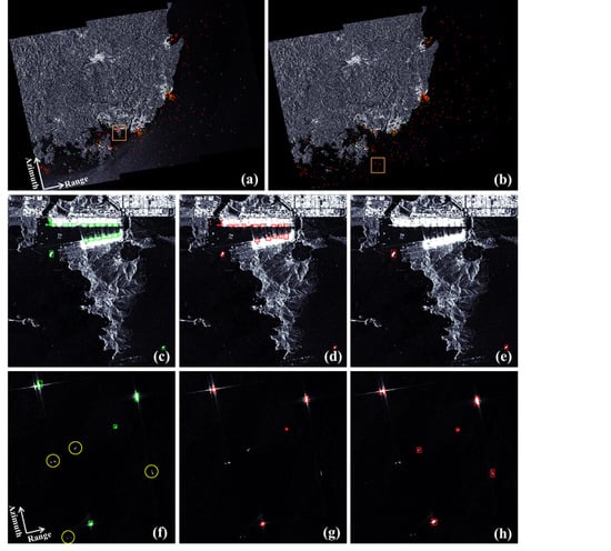
The detection results in Table 2 suggested that the performance of the object detection model implementing training data obtained using the proposed algorithm, 0.7713 overall and 0.7916 in the particular image, significantly exceeded that of training data obtained from visual interpretation, 0.6243 overall and 0.6820 in the particular image. Previous ship detections using SAR images were mostly conducted in different conditions: higher spatial resolution such that superstructure of each ship was discernable [18], covering in open ocean where dislocation of the ship was sparse [33], and having relatively narrow coverage in which included small number of ships compared to this research [15,42]. Under those conditions, the model was able to obtain the overall performance around or higher than 0.9 [15,17,18,19,42] when accompanied by customized detection architecture. This study, however, obtained similar performance with [16], which used two Sentinel-1 images containing 1348 ships with 10 m of spatial resolution for testing while implementing a conventional detection model. Therefore, it could be inferred that the detection performance approximating 0.8 was due to the training dataset from the proposed training data procurement algorithm. Figure 8 illustrates the comparison of detection depending on the training dataset. The magnified region of interest in Figure 8 was selected as inshore region (Figure 8c–e) and the region with severe ghost signals from adjacent ships (Figure 8f–h). The major originality of the research lies on the possibility of discerning ships in port and evading the ghost ambiguity signals from adjacent ships. Accordingly, as the difference between procuring two datasets were concentrated in ships from inshore regions where the ships were difficult to interpret due to a strong scatterer from artificial structures from coastal regions, the detection performance of the AIS-assisted dataset surpassed that from visual interpretation as in Figure 8.
Strong scatterers in the SAR image create ambiguous ghost signals of which the scattering pattern resemble the main signal and separated in certain azimuthal distance equated as,
where denotes azimuthal separation, denotes the order of azimuth ambiguity signal, denotes the pulse repetition interval, denotes the wavelength of the radar system, denotes slant range between the SAR satellite and the scatterer, and denotes the satellite velocity [19]. Given that the offsets between measured azimuthal separations in Figure 8f-h and calculated separations using (17) were bounded around a spatial resolution, four ship-like signals in Figure 8f-h were defined as ghost signals from adjacent ships. Despite the previous studies presented a decline of detection performance in coastal and harbor regions [43] and similarity of the ship and its ghost signals [44], the detection in the regions abided by the overall performance of the full SAR image.
Conventional bottlenecks related to ship detection included (i) detection of AIS deprived vessels, such as illegal fishing ships or ships with martial purposes, (ii) detection of ships with high density of dislocation, especially in inshore regions or pier, (iii) keeping the model from detecting objects, which express high backscattering coefficient besides ships, and (iv) difficulty in procuring mass training data for ships, which is highly time-consuming and inefficient procedure. On the first issue, most ships without AIS information were properly detected by the model, which was trained by AIS-annotated vessels. Secondly, due to the retrieval of training data from near coastal and inshore regions, the model managed to detect a number of ships docked in piers and harbors. In addition, the model was able to discriminate ship lookalikes in coastal regions such as artificial structures in harbors, islands, and sea clusters and excluded those from detection. Azimuth ambiguity ghost signals from ships and land, which may be possible for a chance of appearance in SAR images depending on the pulse repetition interval [19], were also effectively removed from training data construction with respect to AIS signal. Last but not least, the issue of obtaining training data from the satellite image was resolved, as the proposed algorithm suggested the methodology of directly connecting SAR satellite image with AIS information, interpolation of AIS information on proper moment of acquirement, calibrating the offset caused by frequency shift, extraction of bounding box using AIS sensor’s interior position in each vessel and expanding it for proper quantity. When accompanied by AIS information, it was shown that training data for detecting ships could be driven without any intervention of human knowledge.
Current research aroused unresolved obstacles in ship detection. As AIS information was directly derived in the extraction stage, ships with an inaccurate interior position of AIS sensor or even without it may inevitably cause pollution of the training dataset and deterioration of detection performance. The research included the stage of expansion of bounding box for a pixel in every direction to relieve this issue to a certain degree, but it cannot perfectly remove the contamination of bounding box caused by false AIS information. In addition, the effect of each vessel’s artificial structure on construction of SAR images was not considered. The interior structure of the vessel such as bridge, funnel, and forecastle could affect the SAR image during preprocessing and cause expansion of imprinted expression of the ship on SAR images. Accommodation of this effect could be partially conducted by expanding the bounding box to a single pixel, but not be perfected without considering each vessel’s internal structure and geometric conditions. Moreover, due to the relatively low spatial resolution of Sentinel-1 SAR images, ships smaller than a resolution pixel could not be annotated in test images nor easily detected in training images.
Subsequent studies could focus on resolving these limitations of the research. Quantification of the requisite expansion for each bounding box could be determined from additional characters of each ship’s movement. Scattering characteristics of vessels imprinted in SAR imageries could also be mitigated considering their structures, which often depend on their usages. In addition, detailed AIS information of each ship could be used for ship classification, recognizing the ships with respect to their types or usages. This algorithm of implementing AIS information with satellite images could be applied to ship detection in other remote sensing imageries such as optical and infrared images containing ships.
6. Conclusions
This research automated the entire procedure of extracting the bounding box from ships in SAR images by exploiting AIS information without intervention from artificial visual interpretation. Introducing the Kalman filter for accurate prediction on each vessel’s position, restoring satellite orbit for determination and quantification of the Doppler frequency shift and defining the boundary of bounding box using the interior position of the AIS sensor helped create an accurate and renewable procedure of bounding box retrieval. Each bounding box was then expanded by a pixel in every direction considering the effect of rounding in the spatial resolution. Training dataset obtained by applying the proposed extraction methodology and manually extracted training dataset were compared and the results indicated that the proposed method can act as an effective methodology in procuring training data of ships from SAR images, especially from coastal area where ships are not easily discernable by human intelligence. Not only for SAR images, but the proposed methodology can also be applied to ship detection in optical images when leaving the procedure untouched except for the stage of Doppler frequency shift. Further research on this issue includes ship classification as AIS information contains the usage and type of each vessel.
Author Contributions
Conceptualization, D.-j.K.; methodology, J.S., D.-j.K. and K.-m.K.; software, J.S. and K.-m.K.; validation, J.S. and K.-m.K.; formal analysis, J.S.; investigation, J.S.; resources, J.S.; data curation, J.S.; writing—original draft preparation, J.S.; writing—review and editing, J.S., D.-j.K. and K.-m.K.; visualization, J.S.; supervision, D.-j.K.; project administration, D.-j.K.; funding acquisition, D.-j.K. All authors have read and agreed to the published version of the manuscript.
Funding
This study was supported by a grant (no.20009742) of Disaster-Safety Industry Promotion Program funded by Ministry of Interior and Safety (MOIS, Korea) and in part by the “UAV-based Marine Safety, Illegal Fishing and Marine Ecosystem Management Technology Development (no:20190497)” funded by the Ministry of Ocean and Fisheries (MOF, Korea).
Acknowledgments
We thank the Ministry of Oceans and Fisheries (MOF), Korea for providing AIS data. Sentinel-1 data used in this study are provided by ESA through the Sentinel-1 Scientific Data Hub.
Conflicts of Interest
The authors declare no conflict of interest.
References
- Gao, G.; Shi, G. Ship Detection in Dual-Channel ATI-SAR Based on the Notch Filter. IEEE Trans. Geosci. Remote Sens. 2017, 55, 4795–4810. [Google Scholar] [CrossRef]
- Crisp, D.J. The State-of-art in Ship Detection in Synthetic Aperture Radar Imagery. Org. Lett. 2004, 35, 2165–2168. [Google Scholar]
- Rao, N.S.; Ali, M.M.; Rao, M.V.; Ramana, I.V. Estimation of Ship Velocities from MODIS and OCM. IEEE Geosci. Remote Sens. Lett. 2005, 2, 437–439. [Google Scholar]
- Pelich, R.; Longépé, N.; Mercier, G.; Hajduch, G.; Garello, R. AIS-Based Evaluation of Target Detectors and SAR Sensors Characteristics for Maritime Surveillance. IEEE J. Sel. Topics Appl. Earth Observ. Remote Sens. 2015, 8, 3892–3901. [Google Scholar] [CrossRef] [Green Version]
- Velotto, D.; Bentes, C.; Tings, B.; Lehner, S. First Comparison of Sentinel-1 TerraSAR-X data in the Framework of Maritime Targets Detection: South Italy Case. IEEE J. Ocean. Eng. 2016, 41, 993–1006. [Google Scholar] [CrossRef]
- Cumming, I.G.; Wong, F.W. Digital Processing of Synthetic Aperture Radar Data: Algorithms and Implementation. Artech House 2005, 1, 3. [Google Scholar]
- Li, H.; Perrie, W.; He, Y.; Lehner, H.; Brusch, S. Target Detection on the Ocean with the Relative Phase of Compact Polarimetry SAR. IEEE Trans. Geosci. Remote Sens. 2013, 51, 3299–3305. [Google Scholar] [CrossRef]
- Vachon, P.W.; Campbell, J.W.M.; Bjerkelund, C.A.; Dobson, F.W.; Rey, M.T. Ship Detection by the RADARSAT SAR: Validation of Detection Model Predictions. Can. J. Remote Sens. 1997, 23, 48–59. [Google Scholar] [CrossRef]
- Atteia, G.E.; Collins, M.J. On the Use of Compact Polarimetry SAR for Ship Detection. ISPRS J. Photogramm. Remote Sens. 2013, 80, 1–9. [Google Scholar] [CrossRef]
- Velotto, D.; Nunziata, F.; Migliaccio, M.; Lehner, S. Dual-Polarimetric TerraSAR-X SAR Data for Target at Sea Observation. IEEE Geosci. Remote Sens. Lett. 2013, 10, 1114–1118. [Google Scholar] [CrossRef]
- Brekke, C.; Anfinsen, S.N.; Larsen, Y. Subband Extraction Strategies in Ship Detection with the Subaperture Cross-Correlation Magnitude. IEEE Geosci. Remote Sens. Lett. 2013, 10, 786–790. [Google Scholar] [CrossRef] [Green Version]
- Marino, A.; Sanjuan-Ferrer, M.J.; Hajnsek, I.; Ouchi, K. Ship Detection with Spectral Analysis of SAR: A Comparison of New and Well-Known Algorithms. Remote Sens. 2015, 7, 5416–5439. [Google Scholar] [CrossRef]
- Zhu, J.; Qiu, X.; Pan, Z.; Zhang, Y.; Lei, B. An Improved Shape Contexts Base Ship Classification in SAR Images. Remote Sens. 2017, 9, 145. [Google Scholar] [CrossRef] [Green Version]
- Pappas, O.; Achim, A.; Bell, D. Superpixel-Level CFAR Detectors for Ship Detection in SAR Imagery. IEEE Geosci. Remote Sens. Lett. 2018, 15, 1397–1401. [Google Scholar] [CrossRef] [Green Version]
- Hwang, J.; Jung, H. Automatic Ship Detection Using the ANN and SVM from X-band SAR Satellite Images. Remote Sens. 2018, 10, 1799. [Google Scholar] [CrossRef] [Green Version]
- Lin, Z.; Ji, K.; Leng, X.; Kuang, G. Squeeze and Excitation Rank Faster R-CNN for Ship Detection in SAR Images. IEEE Geosci. Remote Sens. Lett. 2019, 16, 751–755. [Google Scholar] [CrossRef]
- Zhang, T.; Zhang, X. High-Speed Ship Detection in SAR Images Based on a Grid-CNN. Remote Sens. 2019, 11, 1206. [Google Scholar] [CrossRef] [Green Version]
- Ma, M.; Chen, J.; Liu, W.; Yang, W. Ship Classification and Detection Based on CNN Using GF-3 SAR Images. Remote Sens. 2018, 10, 2043. [Google Scholar] [CrossRef] [Green Version]
- Wang, J.; Zheng, T.; Lei, P.; Bai, X. A Hierarchical CNN-Based Ship Target Detection Method in Spaceborne SAR Imagery. Remote Sens. 2019, 11, 620. [Google Scholar] [CrossRef] [Green Version]
- Czapiewska, A.; Sadowski, J. Algorithms for Ship Movement Prediction for Location Data Compression. Int. J. Mar. Navig. Saf. Sea Trans. 2015, 9, 75–81. [Google Scholar]
- Zhao, Z.; Ji, K.; Xing, X.; Zou, H.; Zhou, S. Ship Surveillance by Integration of Space-Borne SAR and AIS-Review of Current Research. J. Navig. 2013, 67, 177–189. [Google Scholar] [CrossRef]
- Brusch, S.; Lehner, S.; Fritz, T.; Soccorsi, M.; Soloviev, A.; van Schie, B. Ship Surveillance with TerraSAR-X. IEEE Trans. Geosci. Remote Sens. 2011, 49, 1092–1103. [Google Scholar] [CrossRef]
- Xu, Y.; Lang, H.; Niu, L.; Ge, C. Discriminative Adaptation Regularization Framework-Based Transfer Learning for Ship Classification in SAR images. IEEE Geosci. Remote Sens. Lett. 2019, 16, 1–5. [Google Scholar] [CrossRef]
- Lang, H.; Wu, H.; Xu, Y. Ship Classification in SAR Images Improved by AIS Knowledge Transfer. IEEE Geosci. Remote Sens. Lett. 2018, 15, 439–443. [Google Scholar] [CrossRef]
- Wang, Y.; Wang, C.; Zhang, H. Ship Classification in High-Resolution SAR Images Using Deep Learning of Small Datasets. Sensors 2018, 18, 2929. [Google Scholar] [CrossRef] [Green Version]
- Lu, C.; Li, W. Ship Classification in High-Resolution SAR Images via Transfer Learning with Small Training Dataset. Sensors 2018, 19, 63. [Google Scholar] [CrossRef] [Green Version]
- Huang, L.; Liu, B.; Li, B.; Guo, W.; Yu, W.; Zhang, Z.; Yu, W. OpenSARShip: A Dataset Dedicated to Sentinel-1 Ship Interpretation. IEEE J. Sel. Topics Appl. Earth Observ. Remote Sens. 2018, 11, 195–208. [Google Scholar] [CrossRef]
- Jung, H.; Lu, Z.; Zhang, L. Feasibility of Along-Track Displacement Measurement from Sentinel-1 Interferometric Wide-Swath Mode. IEEE Trans. Geosci. Remote Sens. 2013, 51, 573–578. [Google Scholar] [CrossRef]
- Jakolski, K. AIS Dynamic Data Estimation Based on Discrete Kalman Filter Algorithm. Sci. J. Pol. Nav. Acad. 2017, 4, 211. [Google Scholar]
- Capaldo, P.; Fratarcangeli, F.; Nascetti, A.; Manzzoni, A.; Porfiri, M.; Crespi, M. Centimeter Range Measurement Using Amplitude Data of TerraSAR-X Imagery. In Proceedings of the ISPRS Technical Commission VII Symposium, Istanbul, Turkey, 29 September–2 October 2014; pp. 55–61. [Google Scholar]
- Vachon, P.W.; Campbell, J.W.M.; Gray, A.L.; Dobson, F.W. Validation of Along-Track Interferometric SAR Measurements of Ocean Surface Waves. IEEE Trans. Geosci. Remote Sens. 1999, 37, 150–162. [Google Scholar] [CrossRef]
- Kim, D.; Moon, W.M.; Moller, D.; Imel, D.A. Measurements of Ocean Surface Waves and Currents Using L-and C-Band Along-Track Interferometric SAR. IEEE Trans. Geosci. Remote Sens. 2003, 41, 2821–2832. [Google Scholar]
- Kang, K.; Kim, D. Ship Velocity Estimation from Ship Wakes Detected Using Convolutional Neural Networks. IEEE J. Sel. Topics Appl. Earth Observ. Remote Sens. 2019, 12, 4379–4388. [Google Scholar] [CrossRef]
- Raney, R.K. Synthetic Aperture Imaging Radar and Moving Targets. IEEE Trans. Aerosp. Electron. Syst. 1971, AES-7, 499–505. [Google Scholar] [CrossRef]
- Sengupta, P.; Vadali, S.R.; Alfriend, K.T. Satellite Orbit Design and Maintenance for Terrestrial Coverage. J. Spacecr. Rocket. 2010, 47, 177–187. [Google Scholar] [CrossRef]
- Montenbruck, O. An Epoch State Filter for Use with Analytical Orbit Models of Low Earth Satellites. Aerosp. Sci. Technol. 2000, 4, 277–287. [Google Scholar] [CrossRef]
- Zhou, X.; Yao, C.; Wen, H.; Wang, Y.; Zhou, S.; He, W.; Liang, J. EAST: An Efficient and Accurate Scene Text Detector. In Proceedings of the IEEE Conference on Computer Vision and Pattern Recognition, Honolulu, HI, USA, 21–26 July 2017; pp. 2642–2651. [Google Scholar]
- He, K.; Zhang, X.; Ren, S.; Sun, J. Deep Residual Learning for Image Recognition. In Proceedings of the IEEE Conference on Computer Vision and Pattern Recognition, Las Vegas, NV, USA, 27–30 June 2016; pp. 770–778. [Google Scholar]
- Ai, J.; Tian, R.; Luo, Q.; Jin, J.; Tang, B. Multi-Scale Rotation-Invariant Haar-Like Feature Integrated CNN-Based Ship Detection Algorithm of Multi-Target Environment in SAR Imagery. IEEE Trans. Geosci. Remote Sens. 2019, 57, 10070–10087. [Google Scholar] [CrossRef]
- Li, Q.; Mou, L.; Liu, Q.; Wang, Y.; Zhu, X. HSF-Net: Multiscale Deep Feature Embedding for Ship Detection in Optical Remote Sensing Imagery. IEEE Trans. Geosci. Remote Sens. 2018, 56, 7147–7161. [Google Scholar] [CrossRef]
- Li, X.; Wang, S. Object Detection Using Convolution Neural Network in a Coarse-to-Fine Manner. IEEE Geosci. Remote Sens. Lett. 2017, 14, 2037–2041. [Google Scholar] [CrossRef]
- Hwang, J.; Chae, S.; Kim, D.; Jung, H. Application of Artificial Neural Networks to Ship Detection from X-Band Kompsat-5 Imagery. Appl. Sci. 2017, 7, 961. [Google Scholar] [CrossRef]
- Cui, Z.; Li, Q.; Cao, Z.; Liu, N. Dense Attention Pyramid Networks for Multi-Scale Ship Detection in SAR Images. IEEE Trans. Geosci. Remote Sens. 2019, 57, 8983–8997. [Google Scholar] [CrossRef]
- Chen, J.; Wang, K.; Yang, W.; Liu, W. Accurate Reconstruction and Suppression for Azimuth Ambiguities in Spaceborne Stripmap SAR Images. IEEE Geosci. Remote Sens. Lett. 2017, 14, 102–106. [Google Scholar] [CrossRef] [Green Version]
Figure 1.
Study area and data coverage in vicinity of Korea Strait. Red boxes describe the regions of Sentinel-1 images for training data extraction containing both ascending (Sentinel-1A) and descending (Sentinel-1B) paths.
Figure 1.
Study area and data coverage in vicinity of Korea Strait. Red boxes describe the regions of Sentinel-1 images for training data extraction containing both ascending (Sentinel-1A) and descending (Sentinel-1B) paths.

Figure 2.
Diagram indicating the parameters related to the movement of vessel: (a) the movement of a vessel and (b) the interior position of the automatic identification system (AIS) sensor inside each vessel.
Figure 2.
Diagram indicating the parameters related to the movement of vessel: (a) the movement of a vessel and (b) the interior position of the automatic identification system (AIS) sensor inside each vessel.

Figure 3.
Flowchart of the proposed training data bounding box extraction algorithm using SAR image data and AIS information.
Figure 3.
Flowchart of the proposed training data bounding box extraction algorithm using SAR image data and AIS information.

Figure 4.
Schematic expression of slant range between the SAR satellite and the target ship (), satellite velocity (), and radial velocity ().
Figure 4.
Schematic expression of slant range between the SAR satellite and the target ship (), satellite velocity (), and radial velocity ().

Figure 5.
Descriptions of calculating X, Y, W, and H from the AIS position. Each figure respectively indicates the case where (a) ; (b) ; (c) ; and (d) . (X, Y) denotes the left-upper coordinate of the bounding box, where W and H respectively denotes the width and height of it.
Figure 5.
Descriptions of calculating X, Y, W, and H from the AIS position. Each figure respectively indicates the case where (a) ; (b) ; (c) ; and (d) . (X, Y) denotes the left-upper coordinate of the bounding box, where W and H respectively denotes the width and height of it.

Figure 6.
Schematic overview of the object detection architecture applied for this research.

Figure 7.
Descriptions on the assessment of training data bounding boxes in offshore regions. (a,c) each illustrates the cropped SAR image after binarization implementing threshold and scatterer sorting, where (b,d) respectively describes the green bounding box from the training data procurement from the training data procurement algorithm and red bounding box from the training data assessment algorithm.

Figure 8.
Illustration of contrast between detection results from 2 different training datasets. Green and red bounding boxes respectively denote the ground truth data of ships and the detection results. (a,b) each describes the complete detection result of the target SAR images each taken in 08/07/2018 and 20/07/2018, where orange boxes denotes the coverage of enlarged regions in (c–h), respectively. (d,g) denote the detection using automatically procured training data, where (e,h) denote that from manual training data. Yellow circles in (f) indicate the ghost signals from adjacent ship.


Table 1.
Synthetic aperture radar (SAR) satellite images for training data procurement.
| Satellite | Path | Type, Mode | Acquisition Time (UTC) | Mean Incidence Angle | Usage |
|---|---|---|---|---|---|
| Sentinel-1A | Ascending | GRDH, IW | 26/06/2018 09:23:00~09:23:29 | 38.9605° | Test |
| Sentinel-1A | Ascending | GRDH, IW | 08/07/2018 09:23:00~09:23:29 | 38.9164° | Test |
| Sentinel-1A | Ascending | GRDH, IW | 20/07/2018 09:23:01~09:23:30 | 38.9164° | Test |
| Sentinel-1A | Ascending | GRDH, IW | 01/08/2018 09:23:02~09:23:31 | 38.9327° | Training |
| Sentinel-1A | Ascending | GRDH, IW | 18/09/2018 09:23:04~09:23:33 | 38.9418° | Training |
| Sentinel-1A | Ascending | GRDH, IW | 30/09/2018 09:23:04~09:23:33 | 38.9419° | Training |
| Sentinel-1A | Ascending | GRDH, IW | 12/10/2018 09:23:05~09:23:34 | 38.9397° | Training |
| Sentinel-1A | Ascending | GRDH, IW | 24/10/2018 09:23:05~09:23:34 | 38.9387° | Training |
| Sentinel-1A | Ascending | GRDH, IW | 17/11/2018 09:23:04~09:23:33 | 39.0335° | Training |
| Sentinel-1A | Ascending | GRDH, IW | 29/11/2018 09:23:04~09:23:33 | 38.9633° | Training |
| Sentinel-1A | Ascending | GRDH, IW | 11/12/2018 09:23:03~09:23:32 | 38.9883° | Training |
| Sentinel-1A | Ascending | GRDH, IW | 23/12/2018 09:23:03~09:23:32 | 38.9524° | Training |
| Sentinel-1A | Ascending | GRDH, IW | 16/01/2019 09:23:02~09:23:31 | 38.9532° | Training |
| Sentinel-1B | Descending | GRDH, IW | 12/09/2018 21:23:52~21:24:26 | 39.2235° | Training |
| Sentinel-1B | Descending | GRDH, IW | 24/09/2018 21:23:53~21:24:26 | 39.2208° | Training |
| Sentinel-1B | Descending | GRDH, IW | 18/10/2018 21:23:53~21:24:27 | 39.2183° | Training |
| Sentinel-1B | Descending | GRDH, IW | 30/10/2018 21:23:53~21:24:27 | 39.2175° | Training |
| Sentinel-1B | Descending | GRDH, IW | 11/11/2018 21:23:53~21:24:26 | 39.2173° | Training |
| Sentinel-1B | Descending | GRDH, IW | 23/11/2018 21:23:53~21:24:26 | 39.2174° | Training |
| Sentinel-1B | Descending | GRDH, IW | 05/12/2018 21:23:52~21:24:26 | 39.2170° | Training |
| Sentinel-1B | Descending | GRDH, IW | 17/12/2018 21:23:52~21:24:25 | 39.2165° | Training |
Table 2.
Comparison on the detection performances using two different training datasets.
| Training Data | Acquisition Date | Precision (%) | Recall (%) | F1 Score |
|---|---|---|---|---|
| Automated | Overall | 80.28 | 74.22 | 0.7713 |
| 26/06/2018 | 79.62 | 71.75 | 0.7548 | |
| 08/07/2018 | 82.31 | 76.25 | 0.7916 | |
| 20/07/2018 | 78.74 | 74.26 | 0.7643 | |
| Manual | Overall | 59.03 | 66.24 | 0.6243 |
| 26/06/2018 | 69.50 | 66.95 | 0.6820 | |
| 08/07/2018 | 68.69 | 64.61 | 0.6659 | |
| 20/07/2018 | 46.42 | 67.33 | 0.5495 |
© 2020 by the authors. Licensee MDPI, Basel, Switzerland. This article is an open access article distributed under the terms and conditions of the Creative Commons Attribution (CC BY) license (http://creativecommons.org/licenses/by/4.0/).
Share and Cite
MDPI and ACS Style
Song, J.; Kim, D.-j.; Kang, K.-m. Automated Procurement of Training Data for Machine Learning Algorithm on Ship Detection Using AIS Information. Remote Sens. 2020, 12, 1443. https://doi.org/10.3390/rs12091443
AMA Style
Song J, Kim D-j, Kang K-m. Automated Procurement of Training Data for Machine Learning Algorithm on Ship Detection Using AIS Information. Remote Sensing. 2020; 12(9):1443. https://doi.org/10.3390/rs12091443
Chicago/Turabian StyleSong, Juyoung, Duk-jin Kim, and Ki-mook Kang. 2020. "Automated Procurement of Training Data for Machine Learning Algorithm on Ship Detection Using AIS Information" Remote Sensing 12, no. 9: 1443. https://doi.org/10.3390/rs12091443
Note that from the first issue of 2016, this journal uses article numbers instead of page numbers. See further details here.