YOLOv3-Based Matching Approach for Roof Region Detection from Drone Images
by
 , , ,
, , ,
Chia-Cheng Yeh
1,2 ,
,
Yang-Lang Chang
2,
Mohammad Alkhaleefah
2,
Pai-Hui Hsu
3,
Weiyong Eng
4,
Voon-Chet Koo
4,
Bormin Huang
2,5 and
Lena Chang
6,* 1
National Science and Technology Center for Disaster Reduction, New Taipei 23143, Taiwan
2
Department of Electrical Engineering, National Taipei University of Technology, Taipei 10608, Taiwan
3
Department of Civil Engineering, National Taiwan University, Taipei 10617, Taiwan
4
Faculty of Engineering and Technology, Multimedia University, Melaka 76450, Malaysia
5
The School of Information Science and Technology Southwest Jiaotong University, Chengdu 611756, China
6
Department of Communications, Navigation and Control Engineering, National Taiwan Ocean University, Keelung 20248, Taiwan
*
Author to whom correspondence should be addressed.
Remote Sens. 2021, 13(1), 127; https://doi.org/10.3390/rs13010127
Submission received: 16 November 2020
/
Revised: 19 December 2020
/
Accepted: 21 December 2020
/
Published: 1 January 2021
(This article belongs to the Special Issue GPU Computing for Geoscience and Remote Sensing)
Abstract
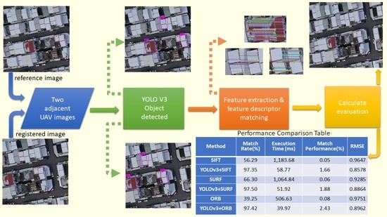
:Due to the large data volume, the UAV image stitching and matching suffers from high computational cost. The traditional feature extraction algorithms—such as Scale-Invariant Feature Transform (SIFT), Speeded Up Robust Features (SURF), and Oriented FAST Rotated BRIEF (ORB)—require heavy computation to extract and describe features in high-resolution UAV images. To overcome this issue, You Only Look Once version 3 (YOLOv3) combined with the traditional feature point matching algorithms is utilized to extract descriptive features from the drone dataset of residential areas for roof detection. Unlike the traditional feature extraction algorithms, YOLOv3 performs the feature extraction solely on the proposed candidate regions instead of the entire image, thus the complexity of the image matching is reduced significantly. Then, all the extracted features are fed into Structural Similarity Index Measure (SSIM) to identify the corresponding roof region pair between consecutive image sequences. In addition, the candidate corresponding roof pair by our architecture serves as the coarse matching region pair and limits the search range of features matching to only the detected roof region. This further improves the feature matching consistency and reduces the chances of wrong feature matching. Analytical results show that the proposed method is 13× faster than the traditional image matching methods with comparable performance.
1. Introduction
Image registration is a traditional computer vision problem for applications in various domains ranging from military, medical, surveillance, robotics, as well as remote sensing [1]. With advances in robotics, cameras can be effortlessly mounted on a UAV to capture the ground images from a top view. A UAV is often operated in a lawn-mower scanning pattern to capture a region of interests (ROI). These captured ROI images are then stitched together to provide an overview representation of the entire region. Drones are relatively low-cost and can be operated in remote areas.
The process of image stitching is useful in a number of tasks, such as disaster prevention, environment change detection, road surveillance, land monitoring, and land measurement. The task of image matching can be divided into two sub-tasks: feature detection and feature description. Researchers have extensively used advanced handcraft feature descriptor algorithms, such as SIFT [2,3], SURF [4,5], and ORB [6]. In the task of feature detection, the distinctive and repetitive features are first detected and input into a non-ambiguous matching algorithm [7,8]. These features are further summarized by region descriptor algorithms such as SIFT, SURF, or ORB. These handcrafted descriptors work by summarizing the histogram of gradient in the region surrounding the feature. SIFT is the pioneer in the work of descriptor handcrafting that is robust to scale and orientation changes. SURF and ORB are approximate and fast versions of SIFT. Features are then matched based on several measures such as brute force matching and Flann-based matching, which is based on the nearest descriptor distance and the matches that satisfy a ratio test as suggested by Lowe et al. [2]. As the raw matches based on these measures often contain outliers, the Random Sample Consensus (RANSAC) [9] is often adopted to perform a match consistency check to filter the outliers. The drone image motion is generally caused by the movement of the camera. Hence, the camera motion can be modeled as a global motion in which every pixel in the image shares a single motion. The global motion is generally modeled as a transformation matrix, which can be estimated by as few as four matching pairs.
Recent advances in deep learning and convolutional neural networks have been applied in various fields such as natural language processing and subsequently in computer vision, especially in the tasks of object detection and object classification [10,11]. The concept of the convolutional neural network was first introduced in LeNet [12]. AlexNet [13] made it well-known after winning the 2012 ImageNet Large-Scale Visual Recognition Challenge (ILSVRC) [14]. Various studies have shown that training a deep network on a large dataset can lead to a better testing accuracy [13,14,15,16]. The advances in the hardware such as the graphics processing unit (GPU) made it possible to process larger data in a shorter time. Recent deep learning methods specifically YOLOv3 [17] have shown consistent good results for object detection and classification.
The most straightforward idea for enhancing the computational time of the drone image registration is the use of high-performance computing (HPC) approach. This study introduces a novel method to integrate the GPU-based deep learning algorithm into traditional image matching methods. The use of a GPU is a significant recent advance for making the training stage of deep network methods more practical [18,19,20,21]. The proposed method generates robust candidate regions by adopting YOLOv3 [17] and performs the traditional image matching only on the candidate regions. Similar to Fast R-CNN [22,23], the use of candidate regions are applied for the image matching tasks instead of image classification.
Structural similarity (SSIM) is then adopted to determine the similarity of the candidates’ regions. The mismatched regions are then filtered and the overlaps are matched to confirm the corresponding relationship of the overlapping regions on two adjacent images. The traditional feature extraction algorithm is then run to extract features from the matched regions and match the features. The search region is thus limited to very small area of the image, reducing the matching error. In the urban, the roof is an important information infrastructure [20]. Therefore, it led to a significant reduction in the computational requirements as the image matching is only performed on the candidate roof regions which is well suited for real-time image registration applications. In this paper, it is shown that our proposed method has achieved 13× faster than the traditional methods of SIFT, SURF, and ORB.
2. Traditional Image Stitching Methods and Deep Learning
Image stitching has been long studied in the fields of computer vision and remote sensing. Traditional image matching methods involve handcrafting descriptors that are robust to photometric and geometric variations at some distinctive repetitive feature locations. The computational cost of the image stitching process rises linearly with the image size as more features are detected and matched for the image stitching. Recent advances in convolutional neural networks and deep learning have shown remarkable results in the field of language processing and image processing. Deep learning has revolutionized high-level computer vision tasks such as object detection and classification. However, further research is needed on adapting deep learning methods in low-level computer vision tasks such as image matching.
2.1. Traditional Image Matching
Traditional image matching methods can be classified as feature-based or pixel-based matching. For drone image registration, the motion is only caused by the movement of the drone. This motion can be approximated by only a single global motion, shared by all the pixels in the image. Hence, feature-based matching is popular in drone image registration. Moreover, feature-based matching is robust to photometric and geometric variations. Only a few distinctive repetitive feature points are detected, and their descriptors are matched. Well-known feature detection methods include the Harris corner detector [7], Hessian affine region detector [24], and Shi Tomasi feature detector [8]. Feature descriptors are handcrafted, such as SIFT [2], SURF [4], and ORB are based on the histogram of gradient (HOG) for a local region surrounding a keypoint location and also the pixel gradient. SIFT [2] is a pioneering feature descriptor, and is the basis for the faster approximate variants SURF [4] and ORB [6].
2.1.1. Scale-Invariant Feature Transform (SIFT)
David Lowe presented the Scale-Invariant Feature Transform (SIFT) algorithm in 1999 [2]. SIFT is perhaps one of the earliest works on providing a comprehensive keypoint detection and feature descriptor extraction technique. The SIFT algorithm has four basic steps.
First, building a multi-resolution pyramid over the input image, and applies difference of Gaussians (DoG), as shown in Equation (1)
In Equation (1), denotes a constant multiplicative factor, .
Secondly, a keypoint localization where the keypoint candidates are localized and refined by eliminating the low contrast points.
Thirdly, to characterize the image at each keypoint, the Gaussian smoothed image L at each level of the pyramid is processed with the closest scale, hence all the computations are performed in a scale-invariant manner. At each pixel L(x,y), the gradient magnitude
and orientation
of the feature points in the image can be calculated as shown in Equation (2) and Equation (3).
The final step of the SIFT algorithm is the local image descriptors where location, scale, and orientation are determined for each keypoint.
2.1.2. Speeded Up Robust Features (SURF)
Herbert Bay et al. presented a novel image feature detection and extraction algorithm called Speeded Up Robust Features (SURF) [4]. SURF is based on the Hessian matrix which can find feature points [4]. Hessian matrix is a square matrix of second-order partial derivatives of a scalar-valued function. It describes the local curvature of a function of many variables. The Hessian matrix measures the local change around each point. It chooses the points at the maximum determinant. Given a point in image I, the Hessian matrix at point and scale
is defined as
where denotes the convolution of the Gaussian second-order derivative
with image I at point ,
, and
are defined similarly. For orientation assignment, it uses wavelet responses in both horizontal and vertical directions by applying adequate Gaussian weights. For feature description also SURF uses the wavelet responses. A neighborhood around the keypoint is selected and divided into subregions and then for each subregion the wavelet responses are taken and represented to get SURF feature descriptor. The sign of Laplacian which is already computed in the detection is used for underlying interest points. The sign of the Laplacian distinguishes bright blobs on dark backgrounds from the reverse case. In matching cases, the features are compared only if they have same type of contrast (based on sign) which allows faster matching [5].
2.1.3. Oriented FAST and Rotated BRIEF(ORB)
Oriented FAST and Rotated BRIEF (ORB) is a computed feature extractor and descriptor algorithm presented by Ethan Rublee [6].
ORB is a fusion of the FAST keypoint detector and BRIEF descriptor with some modifications. Initially to determine the keypoints, it uses FAST, as shown in Equation (5).
FAST corner detector uses a circle of 16 pixels to classify whether a candidate point p is actually a corner or not. Each pixel in the circle is labeled from integer number 1 to 16 clockwise.
is the intensity of candidate pixel p. is the intensity of number 1 to 16. Corner Response Function () gives a numerical value for the corner strength at a pixel location based on the image intensity in the local neighborhoods. The is a threshold intensity value. Then a Harris corner measure is applied to find top N points among them. FAST does not compute the orientation and is rotation variant. It computes the intensity weighted centroid of the patch with located corner at center. The direction of the vector from this corner point to centroid gives the orientation. Moments are computed to improve the rotation invariance. The descriptor BRIEF poorly performs if there is an in-plane rotation. In ORB, a rotation matrix is computed using the orientation of patch and then the BRIEF descriptors are steered according to the orientation [6].
2.1.4. RANdom SAmple Consensus (RANSAC)
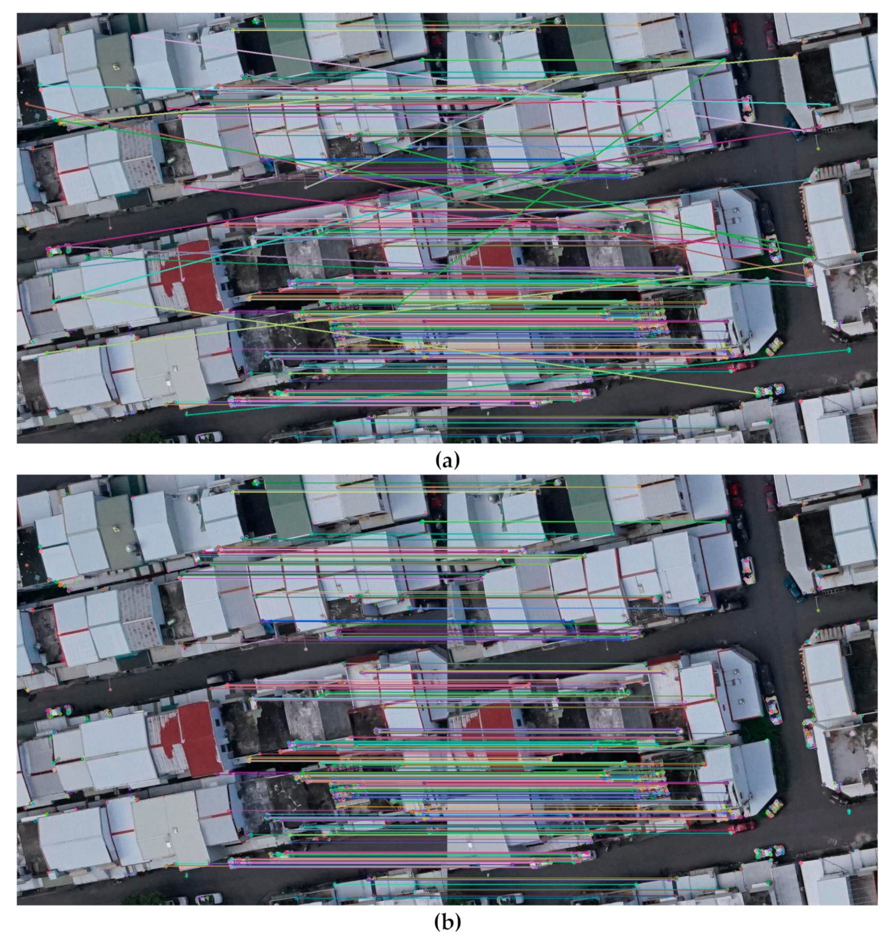
These descriptors between image pairs are then matched against each other to identify the best match with the minimum distance by brute force method. As the matches often contain outliers, a consistency check such as RANSAC [9] is often used to remove inconsistent matches. Figure 1 shows the match points of an input image pair after adopting the RANSAC algorithm [9]. The consistent matches are then used to model a transformation matrix for estimating a global motion for every pixel.
2.2. Deep Learning Algorithms
The development of neural networks-based systems have drastically increased and demonstrated extraordinary performance [22]. The neural networks-based methods have recently emerged as potential alternatives to the traditional methods [24,25]. The recent success of deep learning in computer vision has led to the adoption of the convolutional neural network (CNN) in low-level computer vision tasks such as image matching. Hardware advances such as GPU enable training of a very deep CNN that incorporates hundreds of layers [11].
Object Detection Network
Most current object detection frameworks are either one-stage or two-stage. Regions with convolutional neural network (R-CNN) [26], fast R-CNN [22], and faster R-CNN [27,28] are two-stage object detection frameworks. Two-stage object detectors often achieve high object detection accuracy at a high computational cost. One-stage object detectors, including single shot multibox detector (SSD) [29] and YOLOv3 [17], they formulate the object detection of an input image as a regression problem that outputs class probabilities as well as bounding box coordinates. One-stage object detectors have gained popularity recently, as they achieve comparable object detection accuracy and better speed than two-stage object detectors. Specifically, YOLOv3 [17] has reported achieving consistent high accuracy in object detection. On a Pascal Titan X, YOLOv3 [17] runs in real time at 30 FPS, and has a mAP-50 of 57.9% on COCO test-dev.
3. Proposed Method
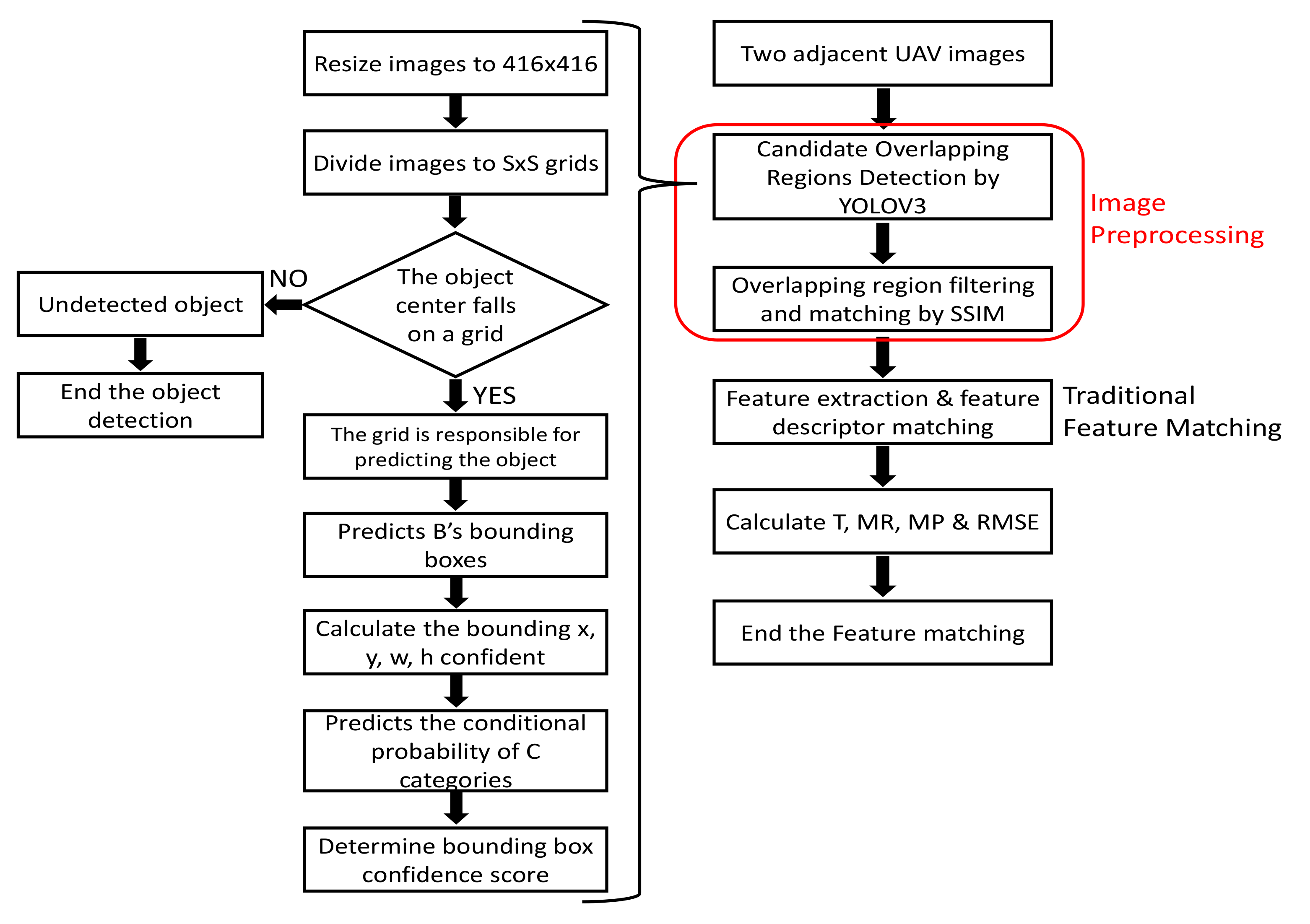
This study presents a novel method to generate a few plausible candidate regions using YOLOv3 [17] object detection for two subsequent drone images on NVIDIA TITAN Xp. The proposed method performs traditional image matching procedures, such as feature extraction and description methods, only in the candidate roof region, thus significantly reducing complexity compared to conventional methods (such as SIFT [2], SURF [4], and ORB [6]). Figure 2 shows the complete flow chart of the algorithm.
All the default YOLOv3 [17] parameter settings were applied, except that the network was only trained for a single class “roof”. The image was divided into S × S grid cells of 13 × 13, 26 × 26 and 52 × 52 for detection on the corresponding scales. Each grid cell is responsible for outputting three bounding boxes, B = 3. Each bounding box outputs five parameters x, y, w, h, and confidence (refers Equation (6)) which define the bounding box location as well as a confidence score indicating the likelihood that the bounding box contains an object.
denotes the probability that the box contains an object. If a cell has no object, then the confidence scores should be 0, otherwise the confidence score should equal the intersection over union (IOU) between the predicted box and ground truth. IOU is a ratio between the intersection and the union of the predicted boxes and the ground truth boxes, when IOU exceeds the threshold, the bounding box is correct, as shown in Equation (7). This standard is used to measure the correlation between ground truth, and prediction,
; a higher value represents a higher correlation.
IOU is frequently adopted as an evaluation metric to measure the accuracy of an object detector. The importance of IOU is not limited to assigning anchor boxes during preparation of the training dataset but is also very useful when adopting the non-max suppression algorithm for cleaning up whenever multiple boxes are predicted for the same object. The IOU is assigned to 0.5 (the default threshold is usually 0.5), which means that at least half of the ground truth and the predicted box cover the same region. When IOU is greater than 50% threshold, the test case is predicted as containing an object.
Each grid cell is assigned 1 conditional class probability,
, which is the probability that the object belongs to the class “roof” given an object is presence. The class confidence score for each prediction box is then calculated as Equation (8), which gives the classification confidence as well as the localization confidence.
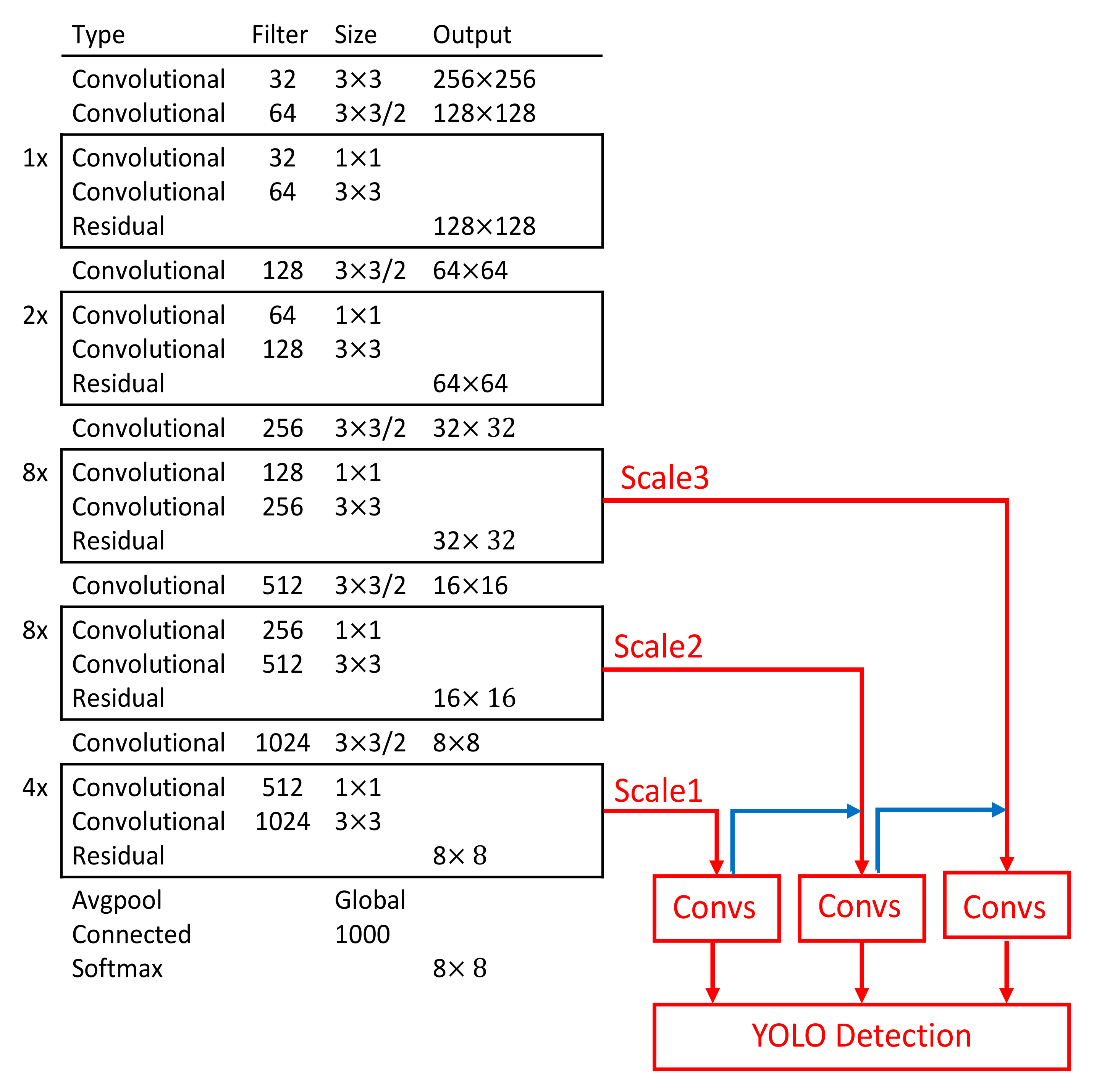
The detection output tensor is of size S × S × B × (5 + C). The value 5 is for the four bounding attributes and one confidence score. Figure 3 shows the detection process using YOLOv3 [17]. Figure 4 shows a backbone network adopted in YOLOv3 [17] for a multiscale object detection. This study adopted the network model for a single class object “roof”. The object “roof” became our candidate regions.
3.1. Dataset and Training Process
3.1.1. Experiment Environment
The experiment environment includes Intel(R) core (TM) i7-8770 @3.2GHz (CPU) and 24 GB of memory, NVIDIA GeForce TITAN Xp GPU with 24 GB memory and using CUDA 9.0. Table 1 shows the hardware and software configurations for the training process.
3.1.2. The Datasets
To evaluate the effectiveness of this research method, we used a set of real images acquired by a UAV equipped with imaging sensors spanning the visible range. The camera is SONY a7R, characterized by a Exmor R full frame CMOS sensor with 36.4 megapixels. All images have been acquired from the National Science and Technology Center for Disaster Reduction, New Taipei, on 13 October 2016, at 10:00 a.m. The images are characterized by three channels (RGB) with 8 bits of radiometric resolution and a spatial resolution of 25 cm ground sample distance (GSD). Table 2 shows the UAV platform and sensor characteristics.
In this study, the dataset comprises 99 drone images with 6000 × 4000 pixel size, captured in the Xizhi District, New Taipei City, Taiwan. As YOLOv3 [17] is designed to train and test the images of 416 × 416 pixel size, the original images were cropped into 1000 × 1000 pixel size with overlapping areas of 70% between the subsequent images. The cropped images were then randomly split into training and testing data at ratio 9:1.
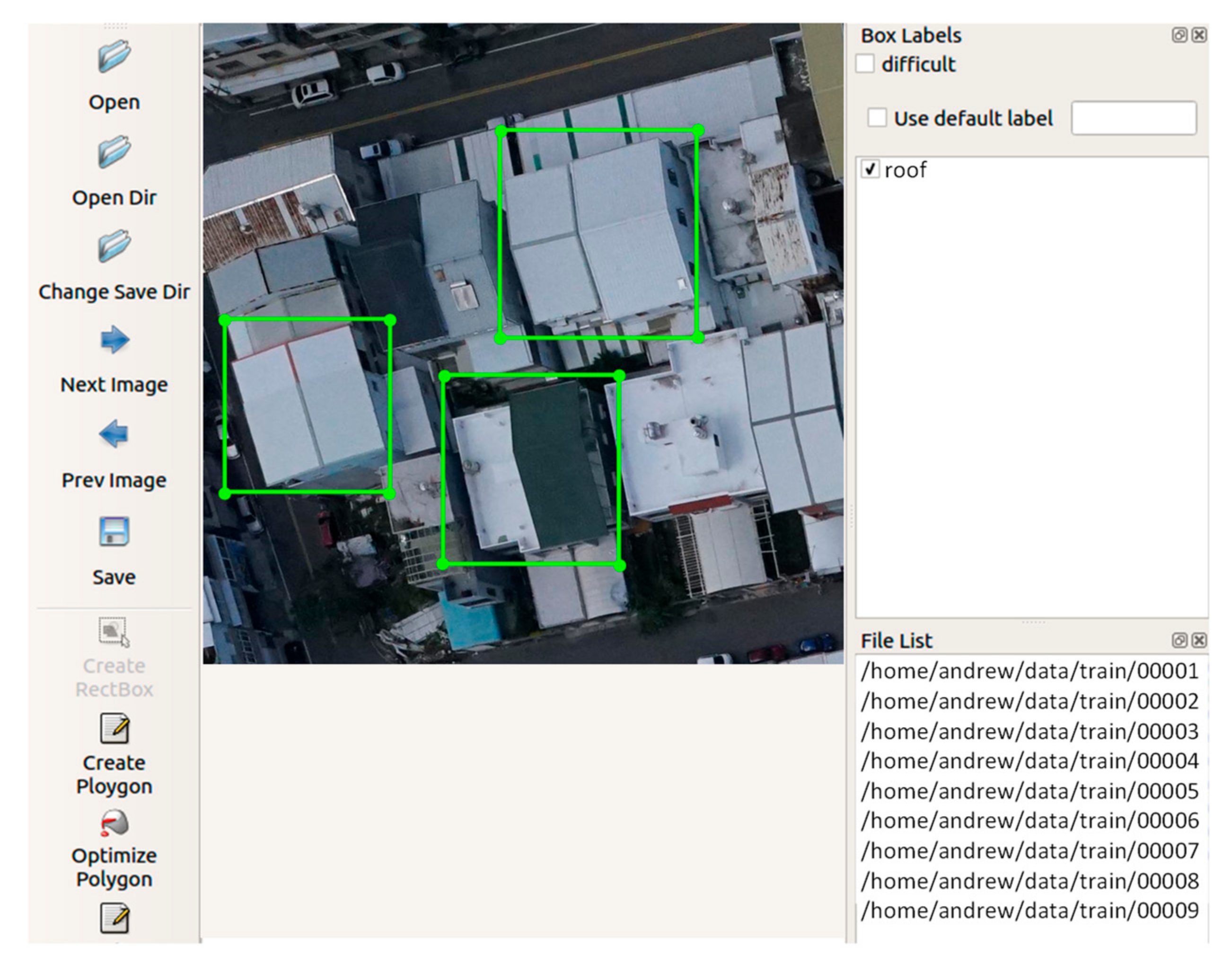
In order to train the network to output the location of the object, all the ground truth objects in the images need to be labeled first. We used the LabelImg open source project on GitHub (tzutalin.github) [29], which is currently the most widely used annotation tool. An open-source software application “LabelImg” [29] was adopted to create the ground truth bounding boxes for the object detection task. Figure 5 shows a screenshot of the process of creating the ground truth bounding boxes using the labelImg software. As the drone images mostly covered the residential areas, only a single class of object “roof” was labeled. The annotations of training images in the XML format were used directly in the YOLOv3 end-to-end training network.
3.2. Evaluation Methods
The precision is the ratio of true positives (true predictions) to the total number of predicted positives
TP denotes the number of true positives. FP denotes the number of false positives and FN is the number of false negatives. The recall is the ratio of true positives to the total of ground truth positives.
The average precision (AP) is the area under the precision–recall curve, and denotes the precision value at .
The loss function is a function that maps an event or value of one or more variables onto a real number intuitively representing some ‘cost’ associated with the event. Therefore, the performance of the training model can be measured by calculating the loss function.
YOLOv3 uses multiple logistic classifiers instead of Softmax to classify each box, since Softmax is not suitable for multi-label classification, and increasing the number of independent multiple logistic classifiers does not decrease the classification accuracy. Therefore, the optimization loss function can be expressed as shown in Equation (12).
In Equation (12), the loss function term1 () calculates the loss related to the predicted bounding box position (x, y). term2 () calculates the loss related to the predicted box width and height (w, h). Terms term3 () and term4 ( ) compute each bounding box predictor and the loss associated with the confidence score.
is the confidence score, and
is the intersection over union of the predicted box with the ground true.
is expressed in Equation (13). The final term () is the classification loss.
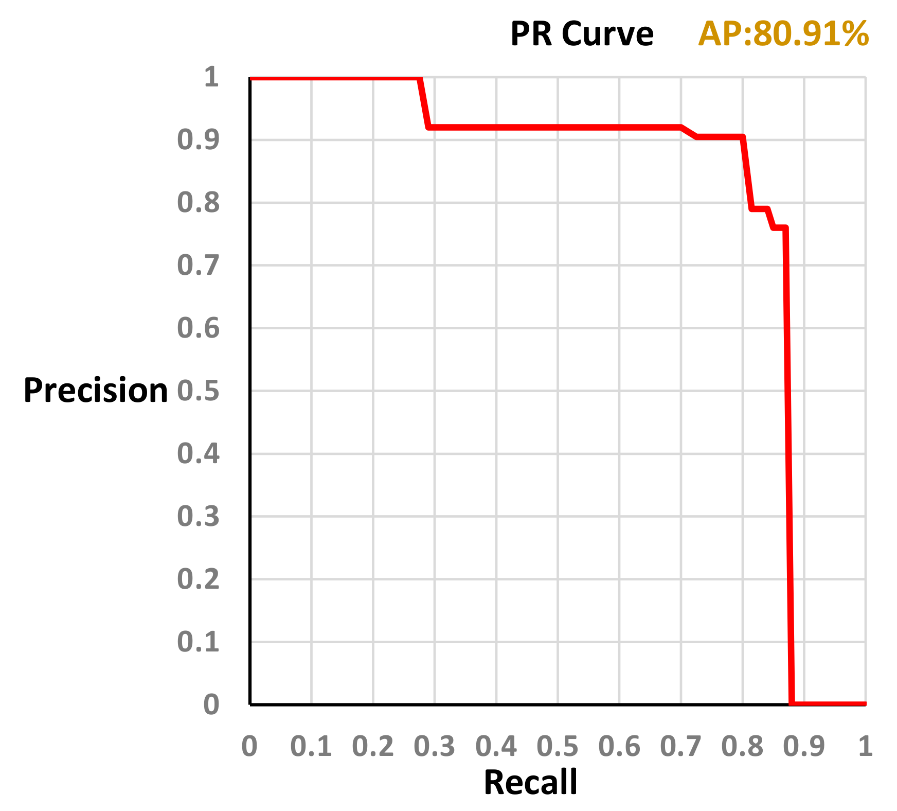
In this study, the dataset comprises 99 drone images. We have used 50 drone images which totally consist of 2200 house roofs divided into 2000 training samples and 200 testing samples. The length of the training time is 4 h. The training time of the deep learning algorithm is excluded from the T computation. Figure 6 shows the precision-recall curve generated by the model trained with our dataset (training sample = 2000, testing sample = 200). The average precision obtained is AP = 80.91%.
3.3. Evaluation and Testing Process
Structural similarity (SSIM) [30] has been used to find the corresponding candidate regions between images in each image pair. Three traditional feature extraction and matching algorithms, SIFT [2], SURF [4], and ORB [6] were then run for image matching within the corresponding candidate regions. The quality of the candidate region pair was evaluated by four evaluation methods, namely, execution time (T) [31,32], match rate (MR) [31,32,33], match performance (MP) [34], and root mean squared error (RMSE) [35,36,37,38]. The execution time (T) measures the algorithms efficiency.
Matching rate (MR) is the ratio between the number of correct matching feature points and the total number of matching feature points detected by the algorithm. In Equation (14), refers to the numbers of keypoints detected in the first and second images respectively, and is the number of matches between these two series of interest points. In Equation (15), we using match performance (MP) to understand the matching status per unit time. In Equation (16), k is the filtered match pair number, where , , and and
are the spatial coordinates of the corresponding matching points on the registration image and the reference image, respectively. A smaller RMSE means a higher registration accuracy, and RMSE < 1 means that the registration accuracy the sub-pixel level.
4. Experimental Results
4.1. Xizhi District, New Taipei City CASE 1
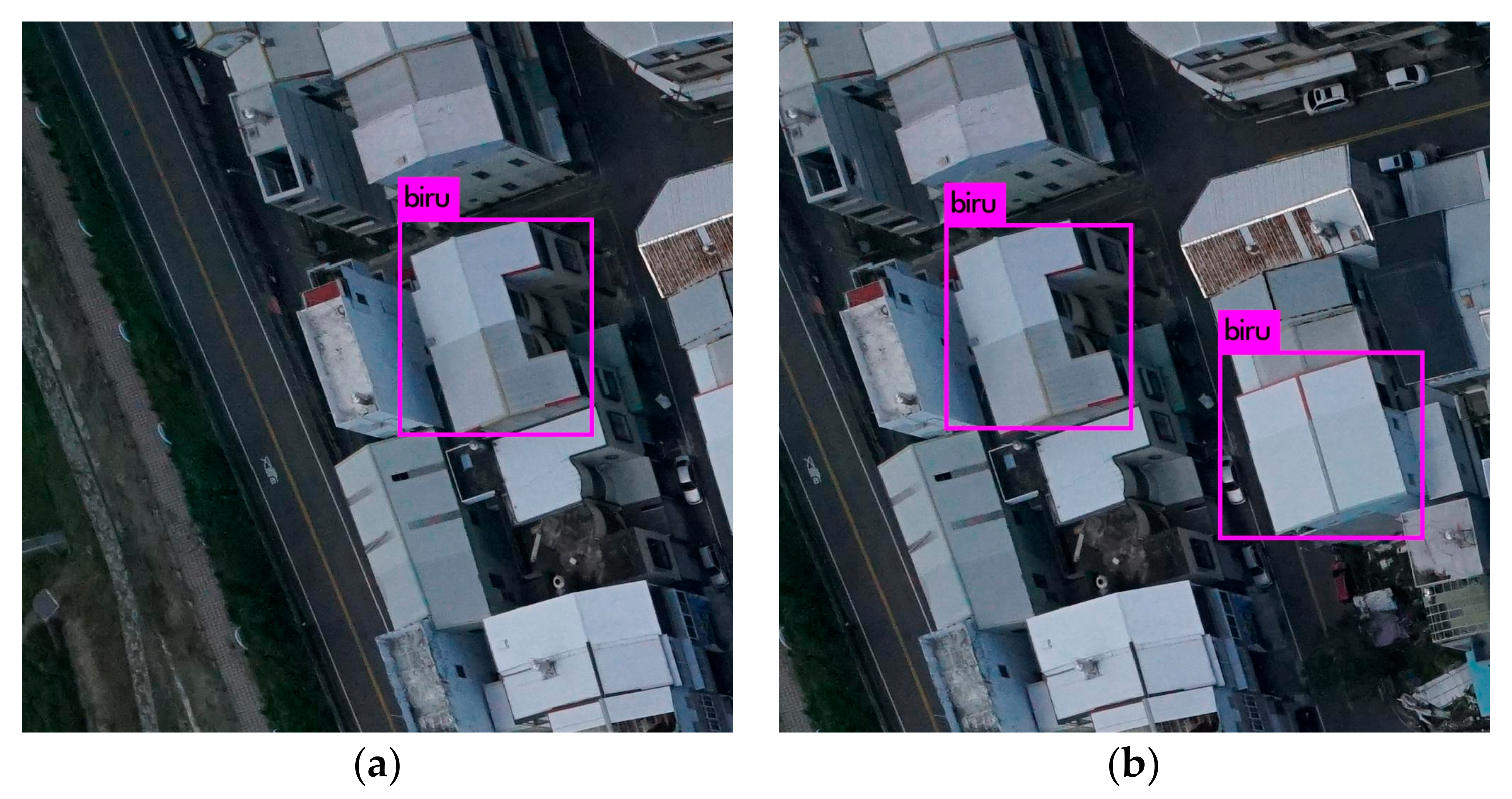
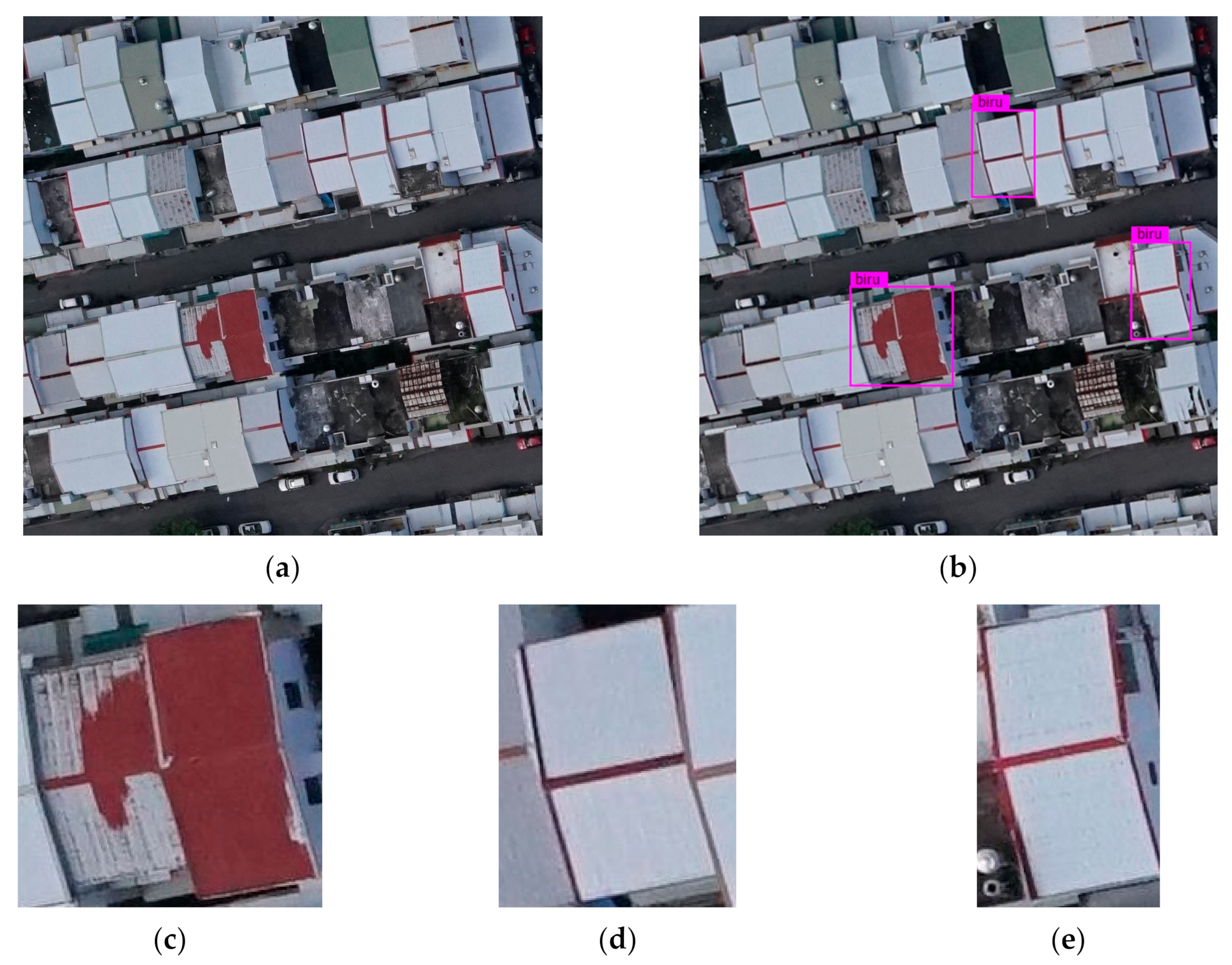
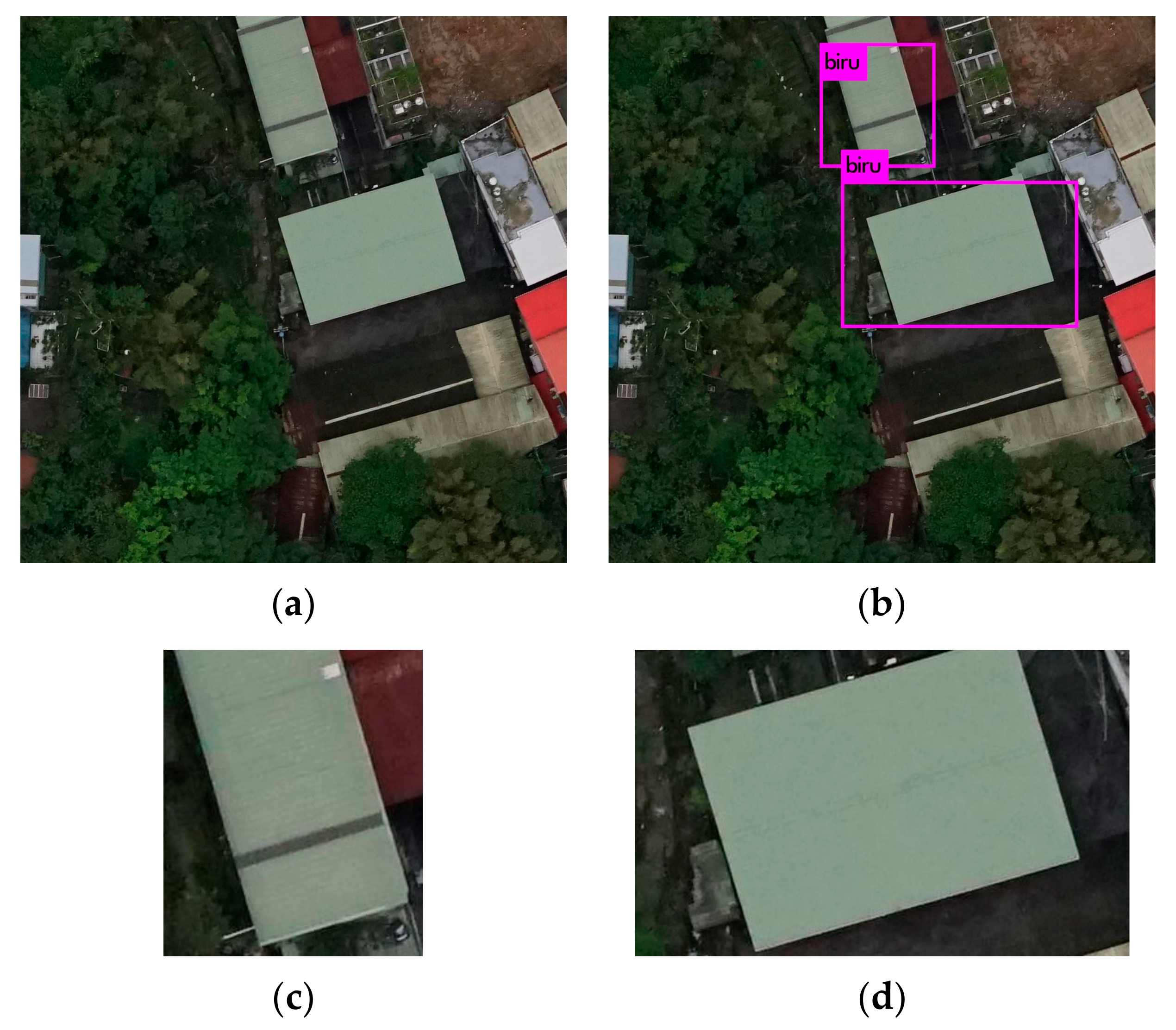
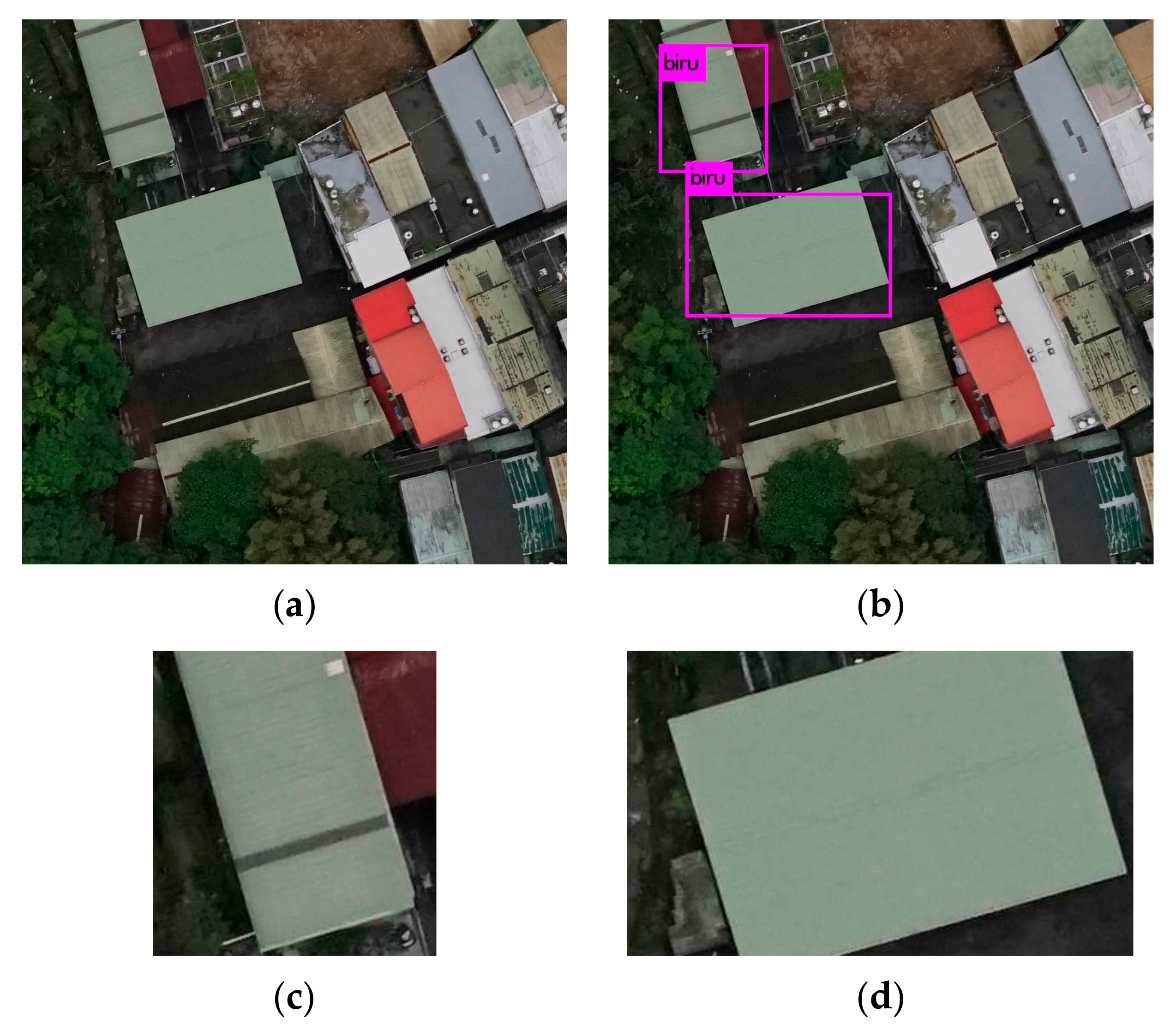
After the training of YOLOv3 is completed, the weights generated after the training can be used to detect the candidate overlapping areas of other UAV images. Figure 8a shows the first image (taken image time = t) that is reference image for the proposed YOLOv3-based roof region detection. Figure 8b, there are three roof regions were detected and highlighted by YOLOv3-based roof region detection. Figure 8c–e shows the candidate regions in the reference image detected by YOLOv3 object detector.
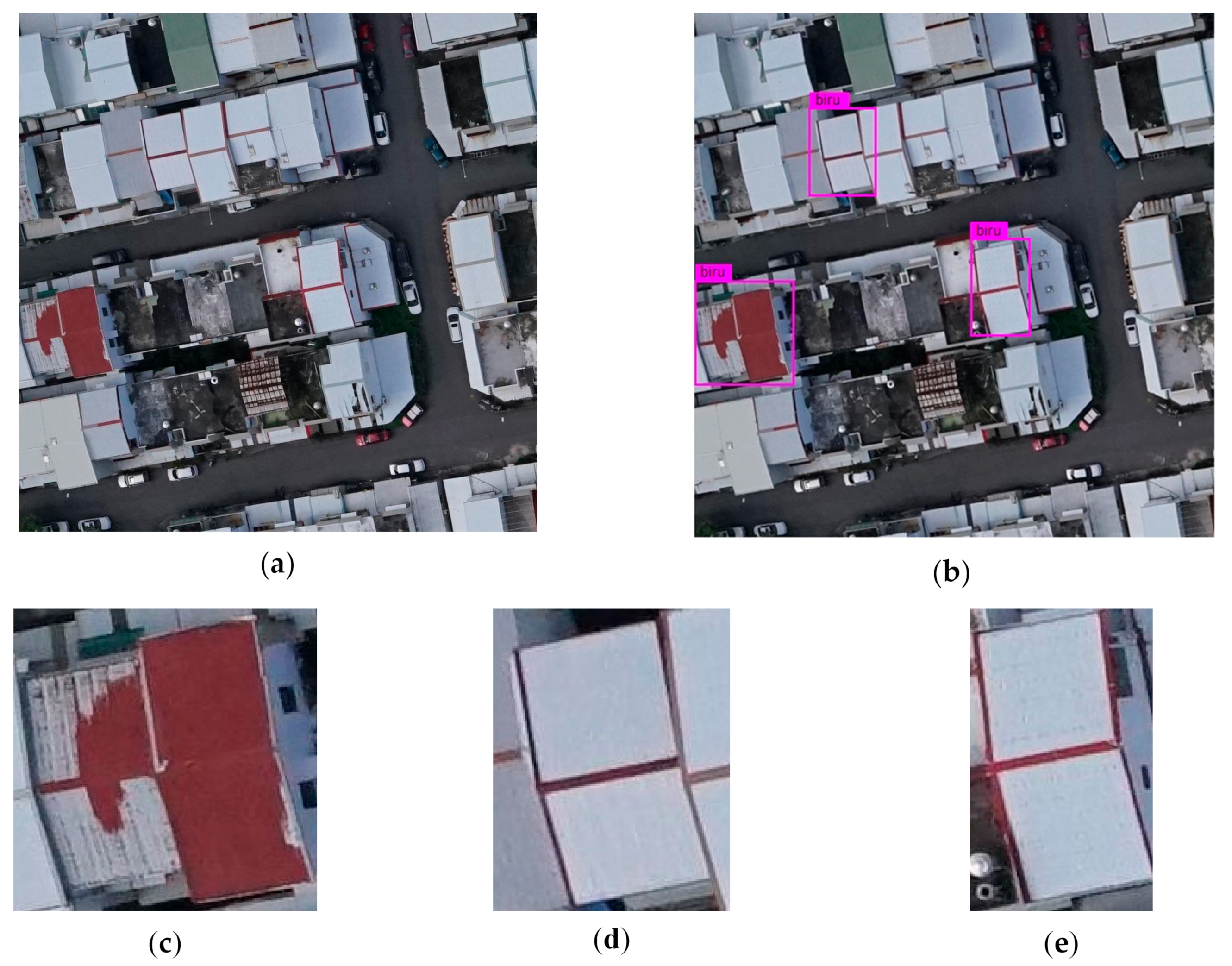
Figure 9a shows the second image (taken image time = t + interval shooting time) that is to be registered for the proposed YOLOv3-based roof region detection. Figure 9b there are three roof regions were detected and highlighted by YOLOv3-based roof region detection. Figure 9c–e shows the candidate regions in the registered image detected by YOLOv3 object detector.
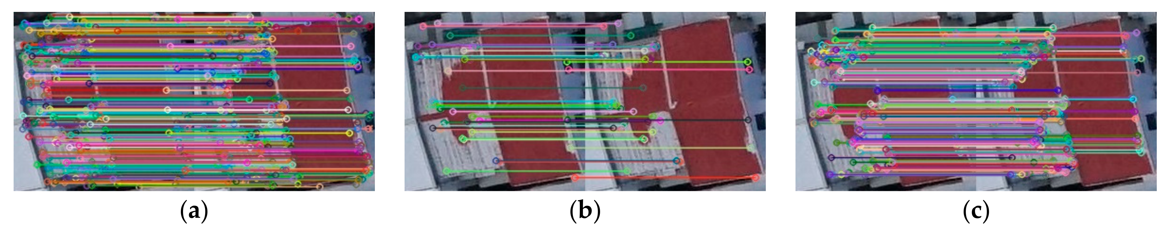
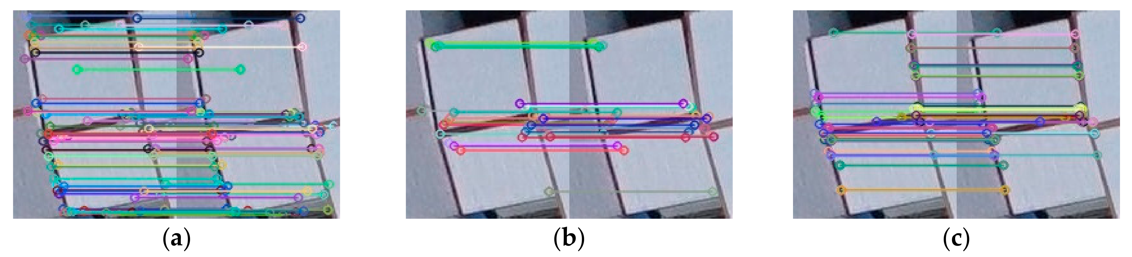
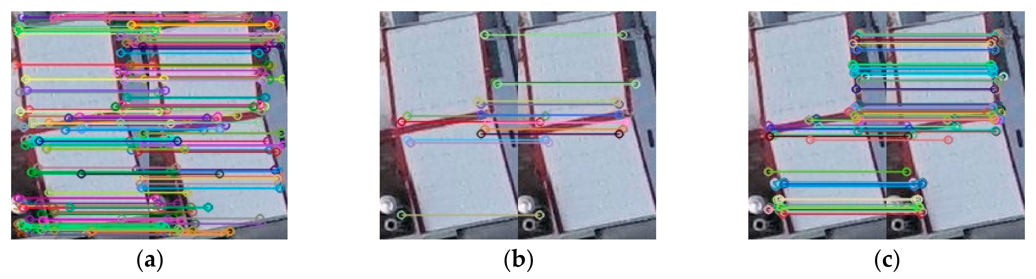
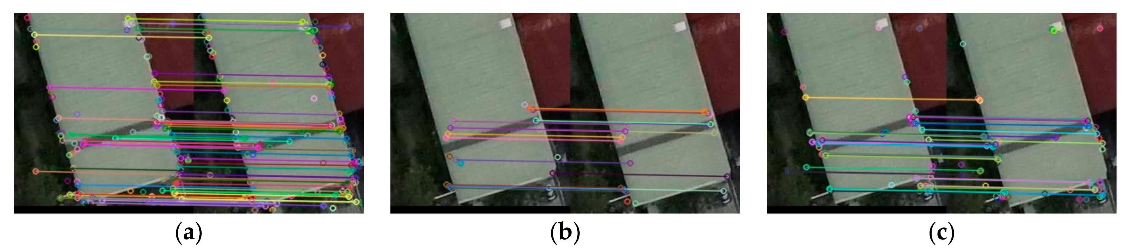
The candidate roof regions were matched to find the corresponding region pair using SSIM [30]. Table 3 shows the SSIM measure between candidate regions and their execution times respectively. After obtaining the corresponding region pairs, traditional feature matching algorithms, SIFT [2], SURF [4], and ORB [6], were performed as shown in Figure 10, Figure 11 and Figure 12 (the right image is registered image, the left image is reference image).
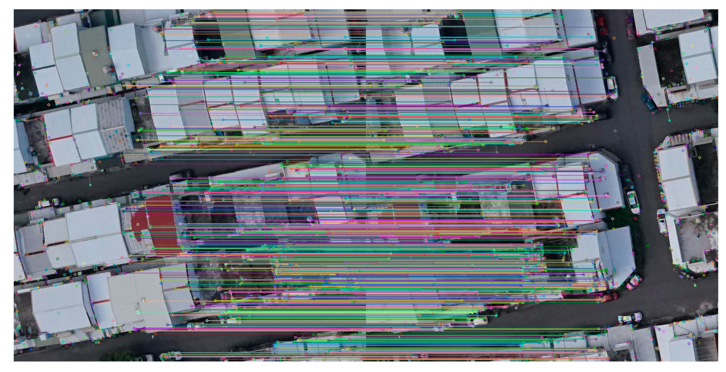
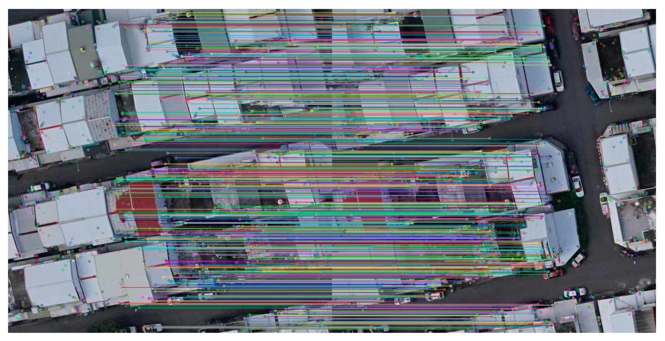
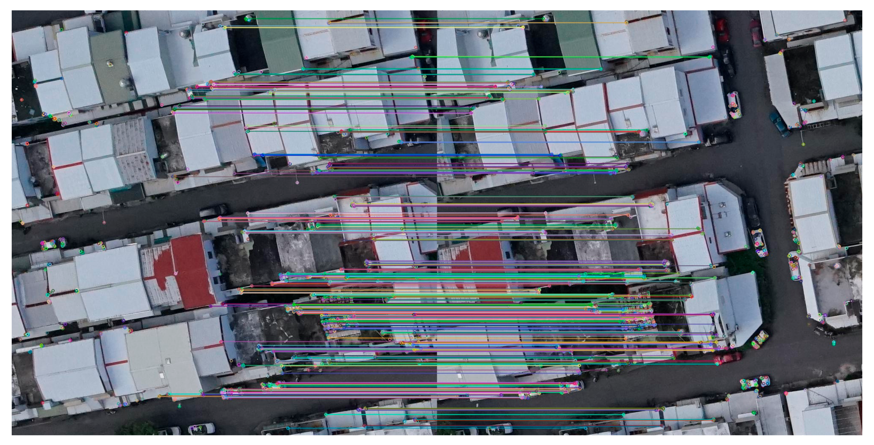
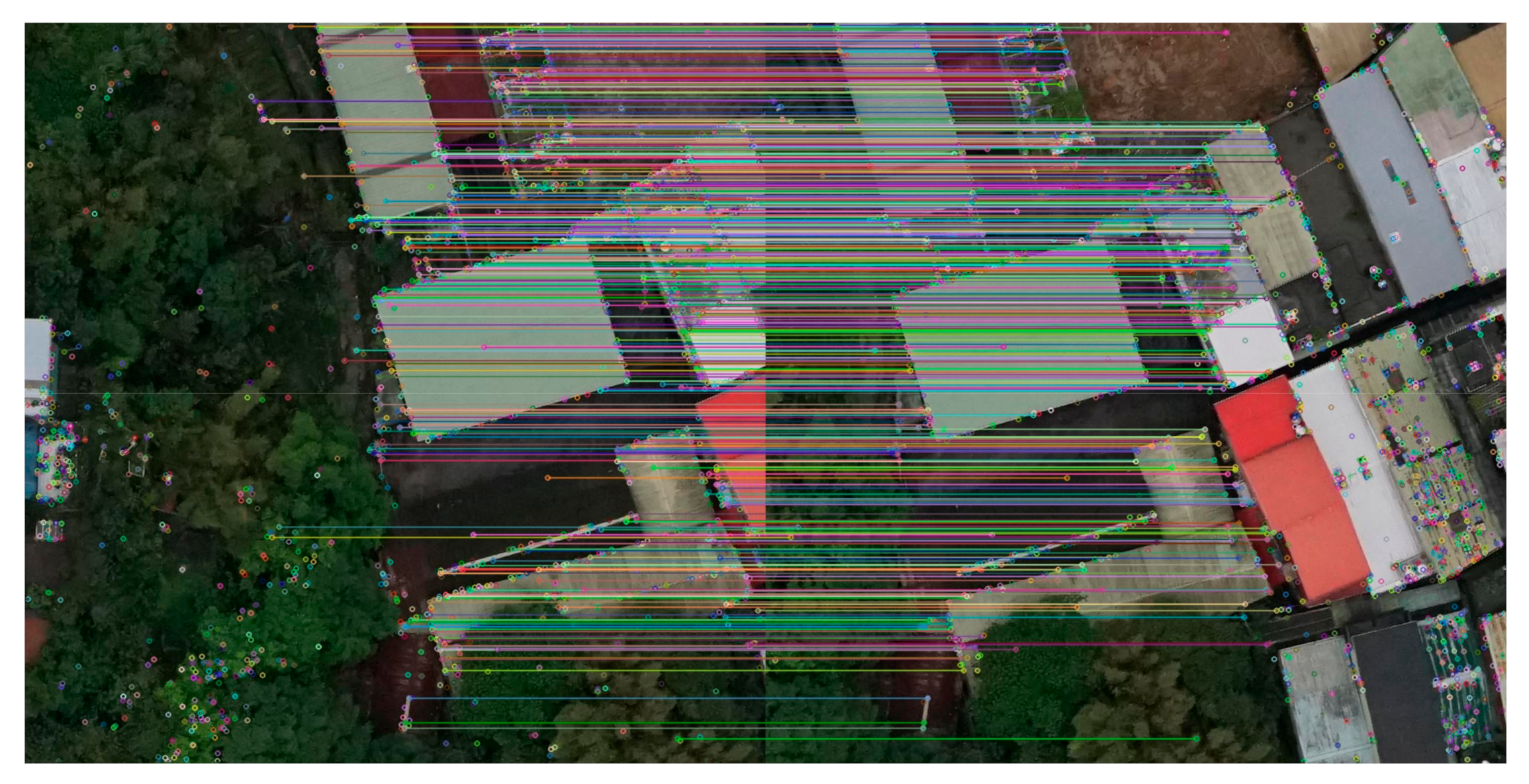
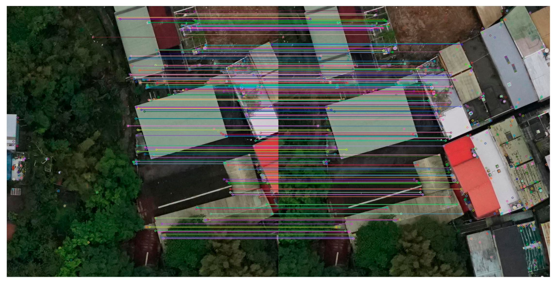
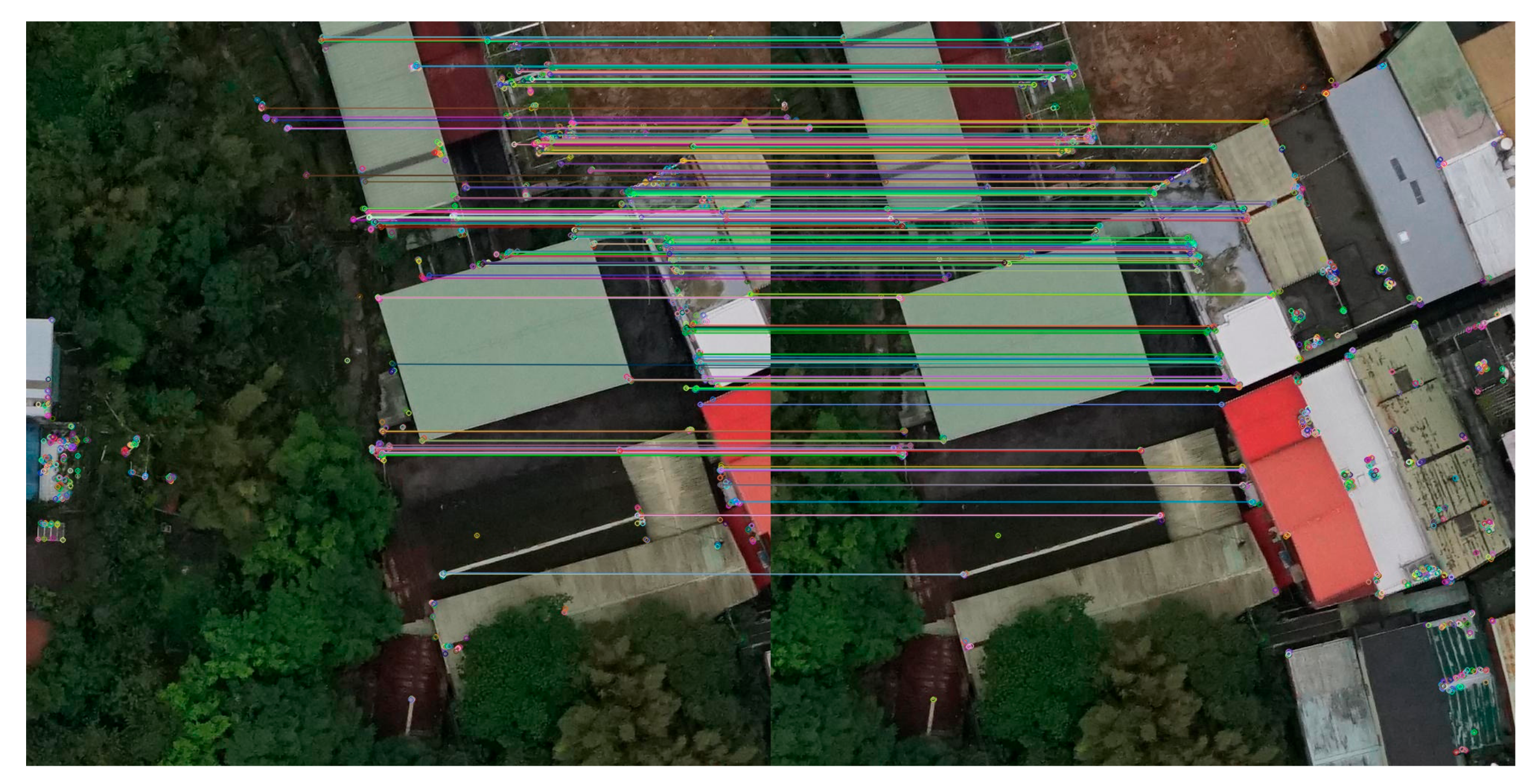
To compare the proposed method with the traditional image matching algorithms, SIFT [2], SURF [4], and ORB [6], feature extraction and matching were performed using these algorithms on the original image pairs, as shown in Figure 13, Figure 14 and Figure 15, respectively. We recorded the number of keypoint, time, and match point coordinates to computed match rate (MR), match performance (MP), and root mean squared error (RMSE).
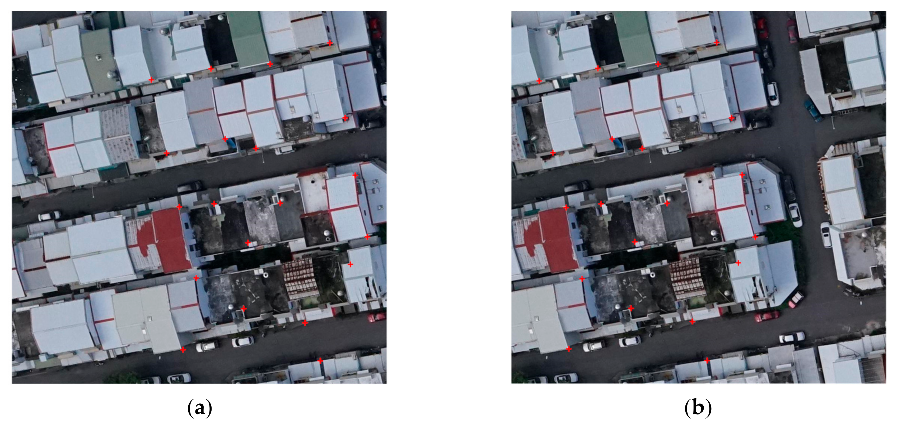
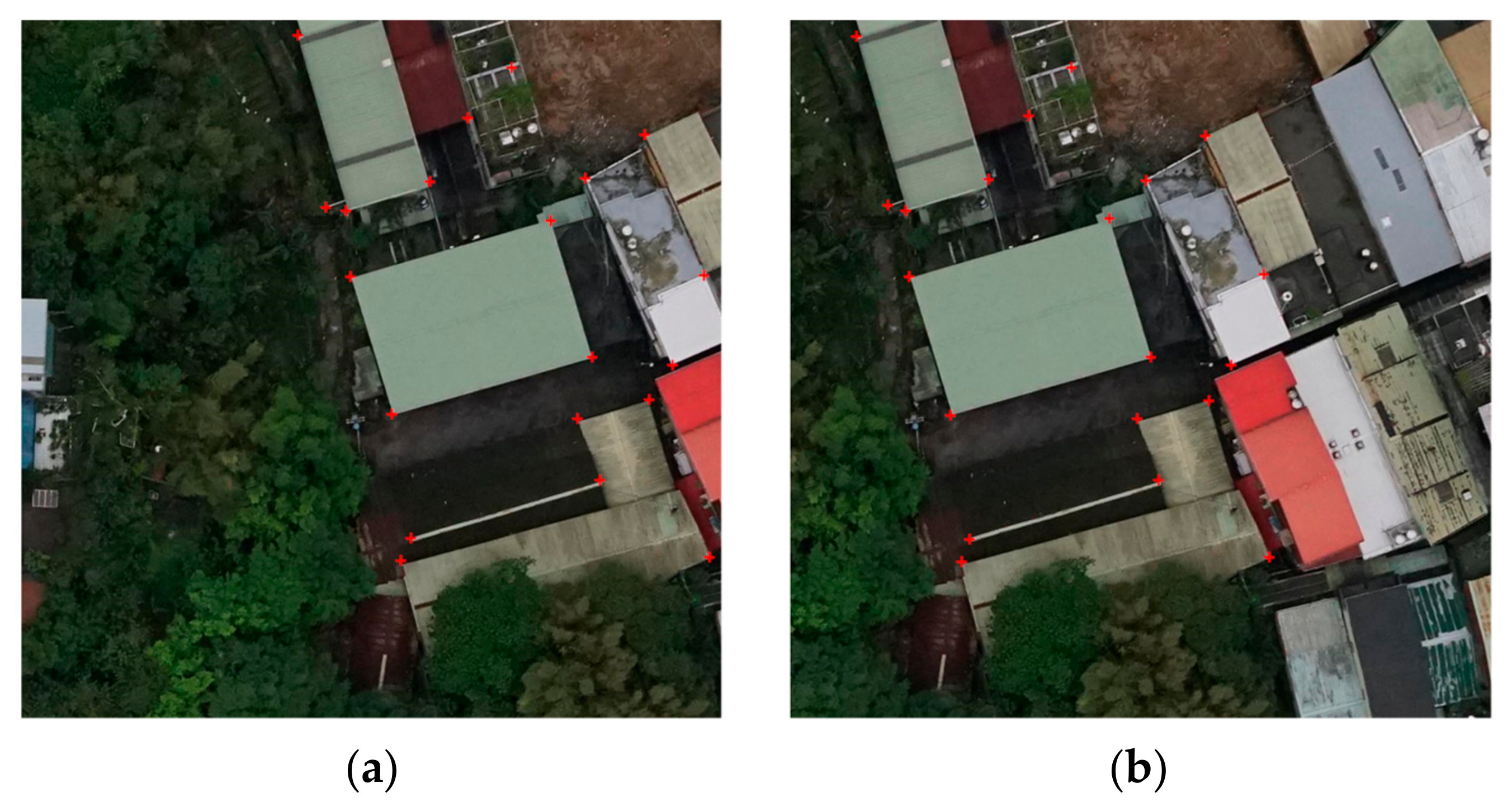
In this paper, we used the ENVI (Environment for Visualizing Images) software to computed the root-mean-squared error (RMSE). The manually selected GCPs (ground control points) combined with match point coordinates used in the root mean squared error (RMSE) calculation. As shown in Figure 16, the 20 pairs of red markers denote the manual selected of GCPs.
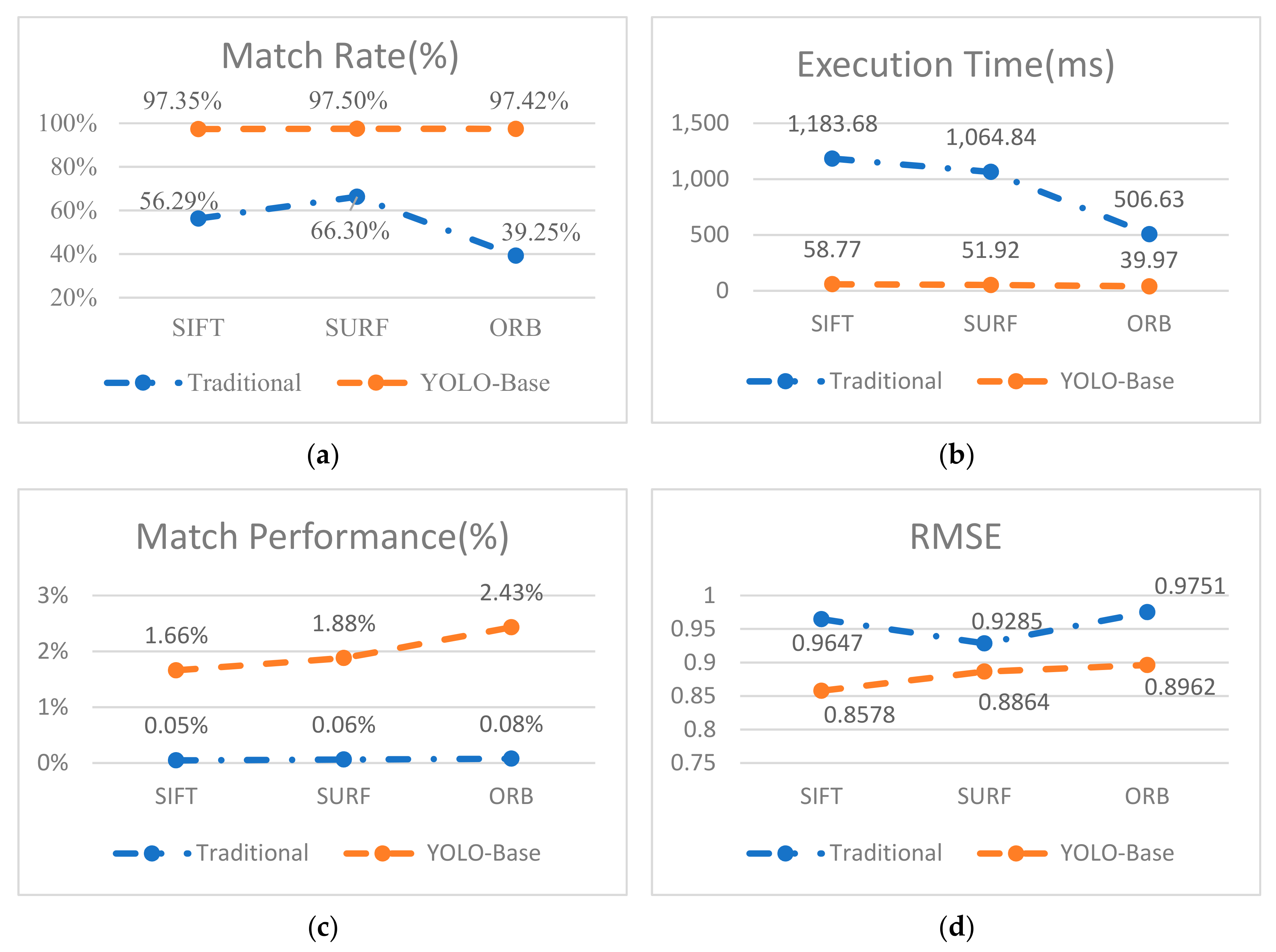
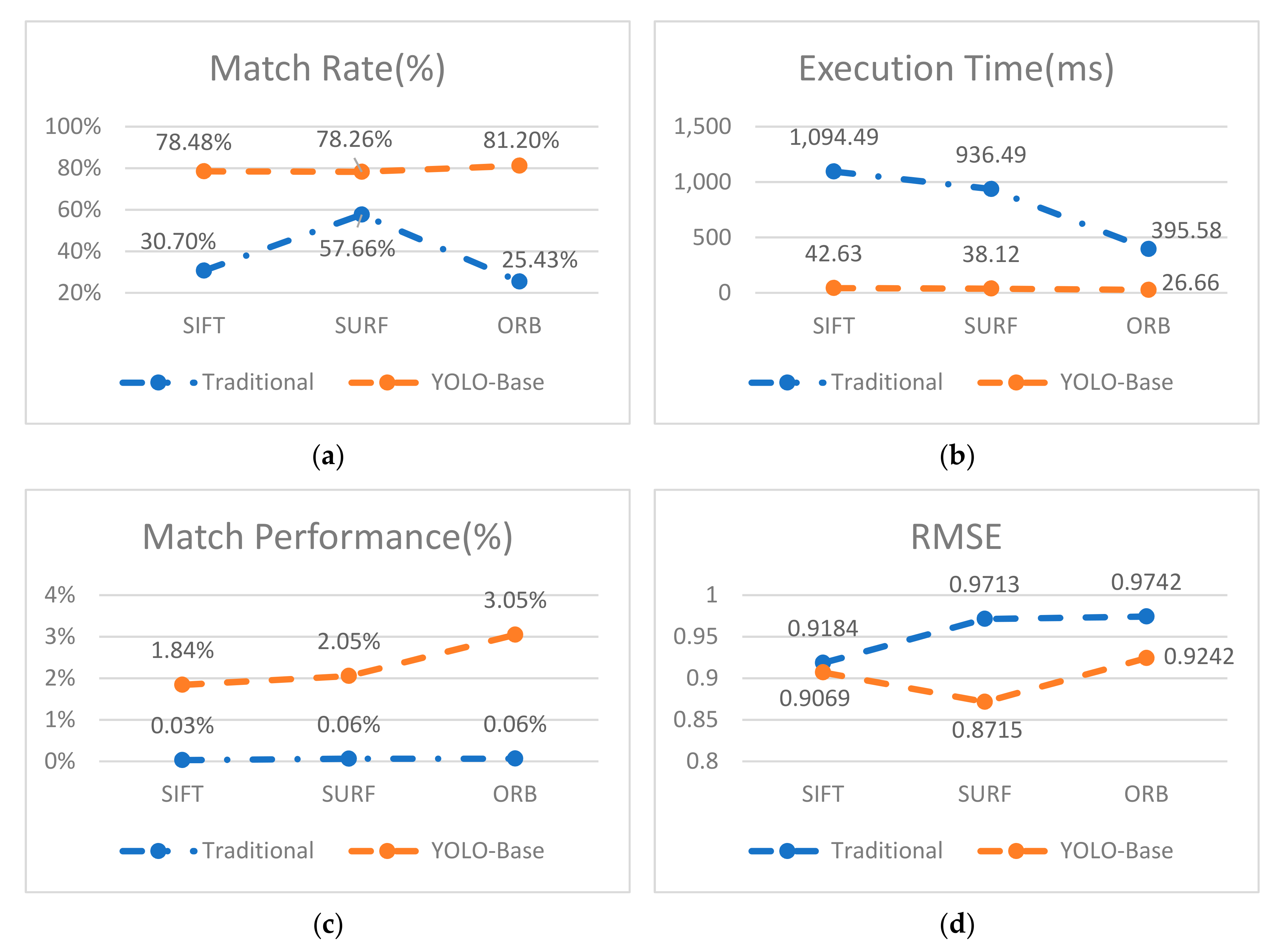
Table 4 and Figure 17 summarize the comparison of traditional image matching algorithms, SIFT [2], SURF [4] and ORB [6], with the YOLOv3-based candidate region matching algorithms YOLOv3+SIFT, YOLOv3+SURF, and YOLOv3+ORB. As shown in Table 4, the proposed method was more than 13× faster compared to the traditional image matching algorithm.
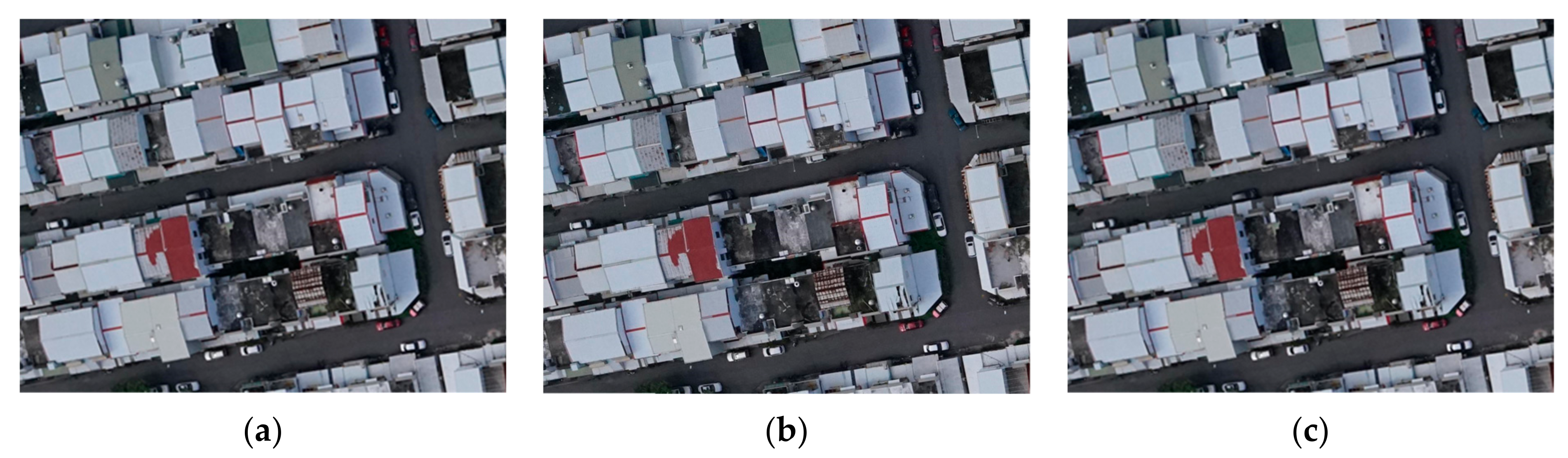
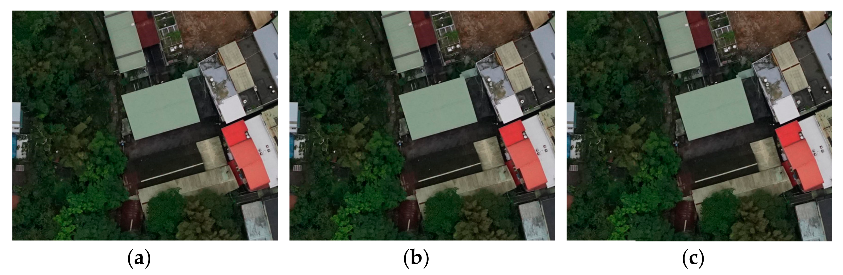
Figure 18 shows the registration result by using the proposed YOLOv3-based matching method.
Our proposed method is compared with the traditional image matching algorithms such as SIFT [2], SURF [4], and ORB [6]. For our quantitative evaluation indexes execution time (T), match rate (MR), match performance (MP), and root mean squared error (RMSE). For the traditional image matching algorithm, the SIFT [2] algorithm had largest number of matching number, it had the longest execution time and lowest match rate. The SURF [4] algorithm’s match rate (MR) and root mean squared error (RMSE) have the best performance among the traditional image matching algorithms. The ORB [6] has the best execution time (T) among the traditional image matching algorithm. As shown in Table 4, experimental results show that the proposed method performance was better than the traditional image matching algorithm. The proposed method can be rapidly implemented and has high accuracy and strong robustness.
4.2. Xizhi District, New Taipei City CASE 2
In this paper, we have evaluated the performance of the YOLOv3-based roof region detection with other cases. Figure 19 shows the reference image and candidate regions in the reference image detected by YOLOv3 object detector.
Figure 20 shows the registered image and candidate regions in the registered image detected by YOLOv3 object detector.
Table 5 shows the SSIM measures between candidate regions and their execution times.
Traditional feature matching algorithms, SIFT [2], SURF [4], and ORB [6], were run on the corresponding region pairs as shown in Figure 21 and Figure 22. The right image is registered image, the left image is reference image.
To compare the proposed method with the traditional image matching algorithms, SIFT [2], SURF [4], and ORB [6] feature extraction and matching were performed on the original image pairs as shown in Figure 23, Figure 24 and Figure 25.
The manually selected GCPs (ground control points) combined with match point coordinates have been collected with the root mean square error (RMSE). As shown in Figure 26.
Table 6 and Figure 27 summarize the comparison between traditional image matching algorithms, SIFT [2], SURF [4], and ORB [6] with the YOLOv3-based candidate region matching algorithms YOLOv3+SIFT, YOLOv3+SURF, and YOLOv3+ORB. As shown in Table 6, the proposed method was more than 15× faster compared to the traditional image matching algorithm.
Figure 28 shows the registration result from the proposed YOLOv3-based matching method. As shown in Table 6, the results show that the proposed method performed was better than the traditional image matching algorithm especially in the execution time (T), where it performs 15× faster than the traditional methods. The proposed method can be rapidly implemented and has high accuracy and strong robustness.
5. Conclusions
Traditional feature-based image matching algorithms dominated the image matching for decades. A fast image matching algorithm is desired as image resolution and size are growing significantly. With the advances of GPU, deep learning algorithms are adopted in various computer vision and language processing fields. In this paper, we proposed a YOLOv3-based image matching approach for fast roof region detection from drone images. As the feature-based matching is performed only on the corresponding region pair instead of the original image pair, the computation complexity is reduced significantly. The proposed approach showed comparable results and performed 13× faster than the traditional methods. In the future work, our model will be trained using overlapping regions with different object conditions. The proposed approach to other UAV images.
Author Contributions
Conceptualization, C.-C.Y. and P.-H.H.; Data curation, C.-C.Y.; Methodology, C.-C.Y., Y.-L.C., P.-H.H., V.-C.K., B.H., and W.E.; Supervision, Y.-L.C., M.A., P.-H.H., B.H., L.C., and V.-C.K.; Validation, C.-C.Y., V.-C.K., and W.E.; Writing—original draft, W.E., M.A., and C.-C.Y.; Writing—review and editing, W.E., C.-C.Y., M.A., V.-C.K., B.H., and Y.-L.C.; C.-C.Y. and Y.-L.C. have the same contributions. All authors have read and agreed to the published version of the manuscript.
Funding
This research received no external funding.
Institutional Review Board Statement
Not applicable.
Informed Consent Statement
Not applicable.
Data Availability Statement
The data presented in this study are available on request from the corresponding author.
Acknowledgments
This work was sponsored by the Ministry of Science and Technology, Taiwan, (grant nos. MOST 108A27A, 108-2116-M-027-003, and 107-2116-M-027-003); National Space Organization, Taiwan, (grant no. NSPO-S-108216); Sinotech Engineering Consultants Inc., (grant no. A-RD-I7001-002), and National Taipei University of Technology, (grant nos. USTP-NTUT-NTOU-107-02, and NTUT-USTB-108-02).
Conflicts of Interest
The authors declare no conflict of interest.
References
- Brown, L.G. A Survey of Image Registration Techniques. ACM 1992, 24, 326–376. [Google Scholar] [CrossRef]
- Lowe, D.G. Object Recognition from Local Scale-Invariant Features. ICCV 1999, 99, 1150–1157. [Google Scholar]
- Lowe, D.G. Distinctive Image Features from Scale-Invariant Keypoints. Int. J. Comput. Vis. 2004, 60, 91–110. [Google Scholar] [CrossRef]
- Bay, H.; Tuytelaars, T.; Van Gool, L. Surf: Speeded up robust features. European Conference on Computer Vision, Graz, Austria, 7–13 May 2006; Springer: New York, NY, USA, 2006; pp. 404–417. [Google Scholar] [CrossRef]
- Bay, H.; Ess, A.; Tuytelaars, T.; Van Gool, L. Speeded-Up Robust Features (SURF). Comput. Vis. Image Underst. 2008, 110, 346–359. [Google Scholar] [CrossRef]
- Rublee, E.; Rabaud, V.; Konolige, K.; Bradski, G.R. ORB: An efficient alternative to SIFT or SURF. In Proceedings of the IEEE International Conference on Computer Vision (ICCV), Barcelona, Spain, 6–13 November 2011; pp. 2564–2571. [Google Scholar]
- Harris, C.G.; Stephens, M.J. A combined corner and edge detector. In Proceedings of the Fourth Alvey Vision Conference, Manchester, UK, 31 August–2 September 1988; pp. 147–152. [Google Scholar]
- Shi, J.; Tomasi, C. Good features to track. In Proceedings of the IEEE Conference on Computer Vision and Pattern Recognition, Seattle, DC, USA, 21–23 June 1994; pp. 593–600. [Google Scholar]
- Fischler, M.A.; Bolles, R.C. Random Sample Consensus: A Paradigm for Model Fitting with Applications to Image Analysis and Automated Cartography. Commun. ACM 1981, 24, 381–395. [Google Scholar] [CrossRef]
- Kamilaris, A.; Prenafeta-Boldú, F.X. Deep Learning in Agriculture: A Survey. Comput. Electron. Agric. 2018, 147, 70–90. [Google Scholar] [CrossRef] [Green Version]
- Liu, L.; Ouyang, W.; Wang, X.; Fieguth, P.; Chen, J.; Liu, X.; Pietikäinen, M. Deep Learning for Generic Object Detection: A Survey. Int. J. Comput. Vis. 2020, 128, 261–318. [Google Scholar] [CrossRef] [Green Version]
- LeCun, Y.; Bottou, L.; Bengio, Y.; Haffner, P. Gradient-Based Learning Applied to Document Recognition. Proc. IEEE 1998, 86, 2278–2324. [Google Scholar] [CrossRef] [Green Version]
- Krizhevsky, A.; Sutskever, I.; Hinton, G.E. Imagenet classification with deep convolutional neural networks. In Proceedings of the 25th Conference on Advances in Neural Information Processing Systems (NIPS), Lake Tahoe, NV, USA, 3–6 December 2012; pp. 1097–1105. [Google Scholar]
- Serre, T. Deep Learning: The Good, the bad, and the Ugly. Annu. Rev. Vis. Sci. 2019, 5, 399–426. [Google Scholar] [CrossRef]
- Simonyan, K.; Zisserman, A. Very Deep Convolutional Networks for Large-Scale Image Recognition. arXiv 2014, arXiv:1409.1556. [Google Scholar]
- He, K.; Zhang, X.; Ren, S.; Sun, J. Deep residual learning for image recognition. In Proceedings of the 2016 IEEE Conference on Computer, Vision, Pattern Recognition, Las Vegas, NV, USA, 27–30 June 2016; pp. 770–778. [Google Scholar]
- Redmon, J.; Farhadi, A. Yolov3: An Incremental Improvement. arXiv 2018, arXiv:1804.02767. [Google Scholar]
- Raina, R.; Madhavan, A.; Ng, A.Y. Large-scale deep unsupervised learning using graphics processors. In Proceedings of the 26th Annual International Conference on Machine Learning, Montreal, QC, Canada, 14–18 June 2009; ACM: Montreal, QC, Canada, 2009; pp. 873–880. [Google Scholar]
- Cire¸san, D.C.; Meier, U.; Gambardella, L.M.; Schmidhuber, J. Deep, Big, Simple Neural Nets for Handwritten Digit Recognition. Neural Comput. 2010, 22, 3207–3220. [Google Scholar] [CrossRef] [PubMed] [Green Version]
- Sugihara, K.; Hayashi, Y. Automatic Generation of 3D Building Models with Multiple Roofs. Tsinghua Sci. Technol. 2008, 13, 368–374. [Google Scholar] [CrossRef]
- Dahl, G.E.; Yu, D.; Deng, L.; Acero, A. Context-Dependent Pre-Trained Deep Neural Networks for Large-Vocabulary Speech Recognition. IEEE Trans. Audio Speech Lang. Process. 2011, 20, 30–42. [Google Scholar] [CrossRef] [Green Version]
- Lee, D.; Lee, S.-J.; Seo, Y.-J. Application of Recent Developments in Deep Learning to ANN-Based Automatic Berthing Systems. Int. J. Eng. Technol. Innov. 2020, 10, 75–90. [Google Scholar] [CrossRef]
- Girshick, R. Fast R-CNN. In Proceedings of the IEEE International Conference on Computer Vision (ICCV), Santiago, Chile, 13–16 December 2015; pp. 1440–1448. [Google Scholar]
- Mikolajczyk, K.; Schmid, C. An affine invariant interest point detector. In Proceedings of the European Conference on Computer Vision, Copenhagen, Denmark, 28–31 May 2002; pp. 128–142. [Google Scholar]
- Zhang, Z.; Geiger, J.; Pohjalainen, J.; Mousa, A.E.; Jin, W.; Schuller, B. Deep Learning for Environmentally Robust Speech Recognition: An Overview of Recent Developments. ACM Trans. Intell. Syst. Technol. 2018, 9, 49:1–49:28. [Google Scholar] [CrossRef]
- Girshick, R.; Donahue, J.; Darrell, T.; Malik, J. Rich feature hierarchies for accurate object detection and semantic segmentation. In Proceedings of the IEEE Conference on Computer Vision and Pattern Recognition, Columbus, OH, USA, 23–28 June 2014; pp. 580–587. [Google Scholar]
- Ren, S.; He, K.; Girshick, R.; Sun, J. Faster R-CNN: Towards Real-Time Object Detection with Region Proposal Networks. IEEE Trans. Pattern Anal. Mach. Intell. 2016, 39, 1137–1149. [Google Scholar] [CrossRef] [Green Version]
- Liu, W.; Anguelov, D.; Erhan, D.; Szegedy, C.; Reed, S.; Fu, C.Y.; Berg, A.C. Ssd: Single shot multibox detector. In Proceedings of the European Conference on Computer Vision—ECCV, Amsterdam, The Netherlands, 8–16 October 2016; pp. 21–37. [Google Scholar]
- Tzutalin. Available online: https://github.com/tzutalin/labelImg (accessed on 30 May 2019).
- Wang, Z.; Bovik, A.C.; Sheikh, H.R.; Simoncelli, E.P. Image Quality Assessment: From Error Visibility to Structural Similarity. IEEE Trans. Image Process. 2004, 13, 600–612. [Google Scholar] [CrossRef] [Green Version]
- Alhwarin, F. Fast and Robust Image Feature Matching Methods for Computer Vision Applications; Shaker Verlag: Aachen, Germany, 2011. [Google Scholar]
- Karami, E.; Prasad, S.; Shehata, M. Image Matching Using SIFT, SURF, BRIEF and ORB: Performance Comparison for Distorted Images. arXiv 2017, arXiv:1710.02726. [Google Scholar]
- Preeti, M.; Bharat, P. An Advanced Technique of Image Matching Using SIFT and SURF. Int. J. Adv. Res. Comput. Commun. Eng. 2016, 5, 462–466. [Google Scholar]
- He, M.M.; Guo, Q.; Li, A.; Chen, J.; Chen, B.; Feng, X.X. Automatic Fast Feature-Level Image Registration for High-Resolution Remote Sensing Images. J. Remote Sens. 2018, 2, 277–292. [Google Scholar]
- Agüera-Vega, F.; Carvajal-Ramírez, F.; Martínez-Carricondo, P. Accuracy of Digital Surface Models and Orthophotos Derived from Unmanned Aerial Vehicle Photogrammetry. J. Surv. Eng. 2016, 143, 4016025. [Google Scholar] [CrossRef]
- Manfreda, S.; Dvorak, P.; Mullerova, J.; Herban, S.; Vuono, P.; Arranz Justel, J.; Perks, M. Assessing the Accuracy of Digital Surface Models Derived from Optical Imagery Acquired with Unmanned Aerial Systems. Drones 2019, 3, 15. [Google Scholar] [CrossRef] [Green Version]
- Gross, J.W.; Heumann, B.W. A Statistical Examination of Image Stitching Software Packages or Use with Unmanned Aerial Systems. Photogramm. Eng. Remote Sens. 2016, 82, 419–425. [Google Scholar] [CrossRef]
- Oniga, V.-E.; Breaban, A.-I.; Statescu, F. Determining the Optimum Number of Ground Control Points for Obtaining High Precision Results Based on UAS Images. Proceedings 2018, 2, 352. [Google Scholar] [CrossRef] [Green Version]
Figure 1.
The match points of an input image pair before and after adopting RANSAC algorithm [9]. (a) initial match, (b) filtered match points.
Figure 1.
The match points of an input image pair before and after adopting RANSAC algorithm [9]. (a) initial match, (b) filtered match points.

Figure 2.
Overall flow chart of the proposed algorithm.

Figure 3.
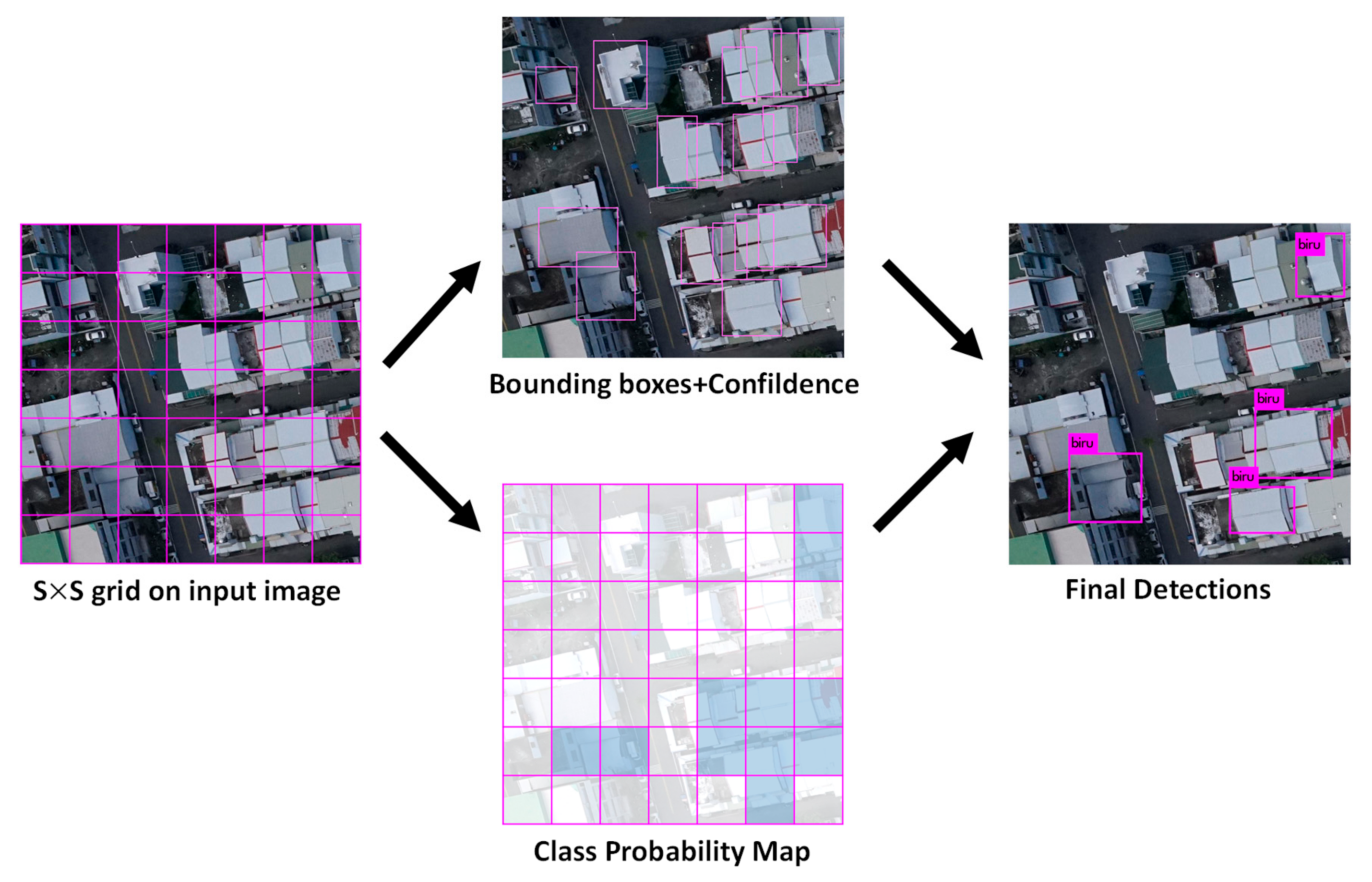
YOLOv3 [17] based model for candidate region. It formulates the candidate region or roof detection as a regression problem. For the illustration purpose, this example has a grid cell size 7 × 7 here. During detection process, the image is first split into S × S size grid cells, and three bounding boxes are estimated for each grid cell. Each bounding box outputs four box attributes indicating its size and location. The final detection is based on the box confidence and class probability.
Figure 3.
YOLOv3 [17] based model for candidate region. It formulates the candidate region or roof detection as a regression problem. For the illustration purpose, this example has a grid cell size 7 × 7 here. During detection process, the image is first split into S × S size grid cells, and three bounding boxes are estimated for each grid cell. Each bounding box outputs four box attributes indicating its size and location. The final detection is based on the box confidence and class probability.

Figure 4.
Backbone network used by YOLOv3 [17] for a three-scale object detection.
Figure 4.
Backbone network used by YOLOv3 [17] for a three-scale object detection.

Figure 5.
LabelImg software interface used to generate the ground truth object labels.

Figure 6.
A precision-recall curve. The average precision obtained is AP = 80.91%.

Figure 7.
Use of two subsequent drone images to perform image matching task by YOLOv3 [17].
Figure 7.
Use of two subsequent drone images to perform image matching task by YOLOv3 [17].

Figure 8.
Drone images were used to perform the image matching task. (a) the reference image, (b) three roof regions were detected and highlighted by YOLOv3-based roof region detection. (c–e) are the candidate regions in the reference image detected by YOLOv3 object detector.
Figure 8.
Drone images were used to perform the image matching task. (a) the reference image, (b) three roof regions were detected and highlighted by YOLOv3-based roof region detection. (c–e) are the candidate regions in the reference image detected by YOLOv3 object detector.

Figure 9.
Drone images were used to perform the image matching task. (a) the image to be registered, (b) three roof regions were detected and highlighted by YOLOv3-based roof region detection. (c–e) are the candidate regions in the registered image detected by YOLOv3 object detector.
Figure 9.
Drone images were used to perform the image matching task. (a) the image to be registered, (b) three roof regions were detected and highlighted by YOLOv3-based roof region detection. (c–e) are the candidate regions in the registered image detected by YOLOv3 object detector.

Figure 10.
Traditional image matching is performed on the candidate roof region pair. The figure shows from left to right: (a) SIFT [2], (b) SURF [4], and (c) ORB [6] feature extraction and matching.

Figure 11.
From left to right: (a) SIFT [2], (b) SURF [4], and (c) ORB [6] feature extraction and matching.

Figure 12.
From left to right: (a) SIFT [2], (b) SURF [4], and (c) ORB [6] feature extraction and matching.

Figure 13.
Traditional image matching by SIFT [2]. The corresponding matched key points are linked by color lines.
Figure 13.
Traditional image matching by SIFT [2]. The corresponding matched key points are linked by color lines.

Figure 14.
Traditional image matching by SURF [4]. The corresponding matched key points are linked by color lines.
Figure 14.
Traditional image matching by SURF [4]. The corresponding matched key points are linked by color lines.

Figure 15.
Traditional image matching by ORB [6]. The corresponding matched key points are linked by color lines.
Figure 15.
Traditional image matching by ORB [6]. The corresponding matched key points are linked by color lines.

Figure 16.
20 pairs of red markers denote the manual selection of ground control points used in the RMSE calculation.
Figure 16.
20 pairs of red markers denote the manual selection of ground control points used in the RMSE calculation.

Figure 17.
Results of four evaluation methods comparing the traditional image matching algorithms with the YOLOv3-based image matching algorithm. (a) Match rate (MR), (b) time (ms), (c) match performance (MP), and (d) root-mean-squared error (RMSE).
Figure 17.
Results of four evaluation methods comparing the traditional image matching algorithms with the YOLOv3-based image matching algorithm. (a) Match rate (MR), (b) time (ms), (c) match performance (MP), and (d) root-mean-squared error (RMSE).

Figure 18.
Registration result of Figure 8a and Figure 9a using: (a) YOLOv3+SIFT, (b) YOLOv3+SURF, (c) YOLOv3+ORB.

Figure 19.
Drone images were used to perform the image matching task. (a) Reference image, (b) three roof regions were detected and highlighted by YOLOv3-based roof region detection. (c,d) are the candidate regions in the reference image detected by YOLOv3 object detector.
Figure 19.
Drone images were used to perform the image matching task. (a) Reference image, (b) three roof regions were detected and highlighted by YOLOv3-based roof region detection. (c,d) are the candidate regions in the reference image detected by YOLOv3 object detector.

Figure 20.
Drone images were used to perform the image matching task. (a) Image to be registered, (b) three roof regions were detected and highlighted by YOLOv3-based roof region detection. (c,d) are the candidate regions in the registered image detected by YOLOv3 object detector.
Figure 20.
Drone images were used to perform the image matching task. (a) Image to be registered, (b) three roof regions were detected and highlighted by YOLOv3-based roof region detection. (c,d) are the candidate regions in the registered image detected by YOLOv3 object detector.

Figure 21.
After the corresponding candidate region was identified between the image pair, traditional image matching was performed on the candidate roof region pair. Figure shows from left to right: (a) SIFT [2], (b) SURF [4], and (c) ORB [6] feature extraction and matching.

Figure 22.
From left to right: (a) SIFT [2], (b) SURF [4], and (c) ORB [6] feature extraction and matching algorithms.

Figure 23.
Traditional image matching by SIFT [2]. The corresponding matched key points are linked by color lines.
Figure 23.
Traditional image matching by SIFT [2]. The corresponding matched key points are linked by color lines.

Figure 24.
Traditional image matching by SURF [4]. The corresponding matched key points are linked by color lines.
Figure 24.
Traditional image matching by SURF [4]. The corresponding matched key points are linked by color lines.

Figure 25.
Traditional image matching by ORB [6]. The corresponding matched key points are linked by color lines.
Figure 25.
Traditional image matching by ORB [6]. The corresponding matched key points are linked by color lines.

Figure 26.
20 pairs of red markers denote the manual selection of ground control points used in the RMSE calculation.
Figure 26.
20 pairs of red markers denote the manual selection of ground control points used in the RMSE calculation.

Figure 27.
Results of four evaluation methods on the traditional image matching algorithms and YOLOv3-based image matching algorithm. (a) Match rate (MR), (b) time (ms), (c) match performance (MP), and (d) root-mean-squared error (RMSE).
Figure 27.
Results of four evaluation methods on the traditional image matching algorithms and YOLOv3-based image matching algorithm. (a) Match rate (MR), (b) time (ms), (c) match performance (MP), and (d) root-mean-squared error (RMSE).

Figure 28.
Registration result of Figure 19a and Figure 20a using: (a) YOLOv3+SIFT, (b) YOLOv3+SURF, (c) YOLOv3+ORB.


Table 1.
Computing hardware and training environment for YOLOv3-based candidate regions.
| Operating System | Ubuntu 16.04 LTS |
| Central processing | Intel i7-8700 3.2GHz |
| Random-access memory (RAM) | DDR4 2400 24GB |
| Graphics card | TITAN Xp (Pascal) |
| Software | Darknet, CUDA9.0 |
Table 2.
UAV platform and sensor characteristics.
| Characteristic Name | Description |
|---|---|
| Platform | ALIAS |
| Flight altitude Above Ground Level (AGL) | 200 m |
| Sensor | SONY a7R |
| Resolution | 7360 × 4912 |
| Output data format | JPEG (Exif 2.3)/ RAW (Sony ARW 2.3) |
| Spatial resolution | 25 cm (GSD) |
| Weather | Overcast |
Table 3.
SSIM between candidate regions to find a matched roof region.
| Figure | SSIM | SSIM Execution Time (ms) |
|---|---|---|
| Figure 8c and Figure 9c | 0.7743 | 3.27 |
| Figure 8c and Figure 9d | 0.6528 | 3.12 |
| Figure 8c and Figure 9e | 0.2644 | 2.83 |
| Figure 8d and Figure 9c | 0.6236 | 3.03 |
| Figure 8d and Figure 9d | 0.8026 | 3.18 |
| Figure 8d and Figure 9e | 0.2836 | 2.91 |
| Figure 8e and Figure 9c | 0.2731 | 3.08 |
| Figure 8e and Figure 9d | 0.2836 | 3.15 |
| Figure 8e and Figure 9e | 0.7263 | 3.22 |
Table 4.
Comparison between the traditional image matching methods and the YOLOv3-based candidate region image matching method for image pair in Figure 8.
Table 4.
Comparison between the traditional image matching methods and the YOLOv3-based candidate region image matching method for image pair in Figure 8.
| Method | Keypoint1 | Keypoint2 | Matches | Match Rate (%) | Execution Time (ms) | Match Performance (%) | RMSE | |
|---|---|---|---|---|---|---|---|---|
| YOLOv3 Time | Matching Time | |||||||
| SIFT | 2000 | 2001 | 1126 | 56.29 | 0 | 1183.68 | 0.05 | 0.9647 |
| YOLOv3+SIFT | 490 | 490 | 477 | 97.35 | 28.98 | 29.79 | 1.66 | 0.8578 |
| SURF | 1582 | 1507 | 1024 | 66.30 | 0 | 1064.84 | 0.06 | 0.9285 |
| YOLOv3+SURF | 80 | 80 | 78 | 97.50 | 28.98 | 22.94 | 1.88 | 0.8864 |
| ORB | 1500 | 1486 | 586 | 39.25 | 0 | 506.63 | 0.08 | 0.9751 |
| YOLOv3+ORB | 619 | 619 | 603 | 97.42 | 28.98 | 10.99 | 2.43 | 0.8962 |
Table 5.
SSIM between candidate region to find a matched roof region.
| Figure | SSIM | SSIM Execution Time (ms) |
|---|---|---|
| Figure 19c and Figure 20c | 0.7143 | 3.53 |
| Figure 19c and Figure 20d | 0.3597 | 3.48 |
| Figure 19d and Figure 20c | 0.4001 | 3.46 |
| Figure 19d and Figure 20d | 0.7688 | 3.58 |
Table 6.
Comparison between traditional image matching methods and the YOLOv3-based candidate region image matching method for image pair in Figure 19.
Table 6.
Comparison between traditional image matching methods and the YOLOv3-based candidate region image matching method for image pair in Figure 19.
| Method | Keypoint1 | Keypoint2 | Matches | Match Rate (%) | Execution Time (ms) | Match Performance (%) | RMSE | |
|---|---|---|---|---|---|---|---|---|
| YOLOv3 Time | Matching Time | |||||||
| SIFT | 2000 | 2000 | 614 | 30.70 | 0 | 1094.49 | 0.03 | 0.9184 |
| YOLOv3+SIFT | 130 | 186 | 124 | 78.48 | 16.72 | 25.91 | 1.84 | 0.9069 |
| SURF | 309 | 520 | 239 | 57.66 | 0 | 936.49 | 0.06 | 0.9713 |
| YOLOv3+SURF | 37 | 32 | 27 | 78.26 | 16.72 | 21.40 | 2.05 | 0.8715 |
| ORB | 1500 | 1496 | 381 | 25.43 | 0 | 295.57 | 0.06 | 0.9742 |
| YOLOv3+ORB | 129 | 105 | 95 | 81.20 | 16.72 | 9.94 | 3.05 | 0.9242 |
Publisher’s Note: MDPI stays neutral with regard to jurisdictional claims in published maps and institutional affiliations. |
© 2021 by the authors. Licensee MDPI, Basel, Switzerland. This article is an open access article distributed under the terms and conditions of the Creative Commons Attribution (CC BY) license (http://creativecommons.org/licenses/by/4.0/).
Share and Cite
MDPI and ACS Style
Yeh, C.-C.; Chang, Y.-L.; Alkhaleefah, M.; Hsu, P.-H.; Eng, W.; Koo, V.-C.; Huang, B.; Chang, L. YOLOv3-Based Matching Approach for Roof Region Detection from Drone Images. Remote Sens. 2021, 13, 127. https://doi.org/10.3390/rs13010127
AMA Style
Yeh C-C, Chang Y-L, Alkhaleefah M, Hsu P-H, Eng W, Koo V-C, Huang B, Chang L. YOLOv3-Based Matching Approach for Roof Region Detection from Drone Images. Remote Sensing. 2021; 13(1):127. https://doi.org/10.3390/rs13010127
Chicago/Turabian StyleYeh, Chia-Cheng, Yang-Lang Chang, Mohammad Alkhaleefah, Pai-Hui Hsu, Weiyong Eng, Voon-Chet Koo, Bormin Huang, and Lena Chang. 2021. "YOLOv3-Based Matching Approach for Roof Region Detection from Drone Images" Remote Sensing 13, no. 1: 127. https://doi.org/10.3390/rs13010127
Note that from the first issue of 2016, this journal uses article numbers instead of page numbers. See further details here.